Heuristic method for relay node placement in heterogeneous wireless network

Whether it is to initially deploy a network or to restore the connectivity in a partitioned one, the question of the optimal Relay Node (RN) placement arises. This problem is already challenging when considering a static homogeneous network. However, diversity in transmission parameters within the network can induce diversity in transmission ranges, imposing the consideration of heterogeneity in the network. Furthermore, if the nodes are moving, the RN placement scheme must manage a smooth repositioning of the RNs without any large jumps or major restructuring. This paper introduces an effective strategy for deploying the minimum number of RNs in order to restore the connectivity between the nodes of a partitioned heterogeneous network. Through the statistical analysis of results from numerous randomly generated scenarios, the proposed Barycenter-focused Relay nodes placement for Heterogeneous wireless Networks (BRHEN) algorithm is shown to be an improvement on other similar approaches in terms of the number of RNs and the latency. Additionally, BRHEN exhibits stability in the positions and number of RNs when small displacements are applied to the Initial Nodes (INs). This characteristic makes this method suitable for scenarios with moving INs.

1 Introduction

Modern wireless networks are inherently heterogeneous, incorporating diverse types of nodes with varying capabilities, communication ranges, and energy constraints. This heterogeneity introduces significant challenges in maintaining network connectivity, optimizing performance, and ensuring efficient data transmission. A critical aspect of network management in such environments is the strategic placement of Relay Nodes (RNs), which serve to improve connectivity, extend network coverage, and enhance overall reliability.

Effective relay node placement becomes particularly crucial in scenarios where network partitions arise due to node failures, mobility, or energy depletion. Conventional relay placement methods often assume homogeneous network conditions, failing to account for the diverse characteristics of nodes present in real-world deployments. However, in heterogeneous networks—such as those found in Internet of Things (IoT) ecosystems, heterogeneous cellular networks (HetNets), and next-generation wireless communication systems (Parihar et al. 2024a; Parihar et al. 2024b; Swami et al., 2022) — a homogeneous approach to RN placement is insufficient. Instead, adaptive placement strategies that consider node diversity, transmission power, and network topology dynamics are essential for maintaining seamless connectivity and optimizing performance.

Given these challenges, an effective relay node placement method that explicitly accounts for network heterogeneity is essential. Existing approaches often fail to fully address the impact of node diversity and mobility on RN deployment strategies, highlighting the need for more adaptive solutions. In the following, we review the current state of research on relay node placement, by examining the methodologies proposed to handle network heterogeneity, and by identifying key gaps that motivate the need for improved strategies.

A wide range of scenarios requiring RN deployment can be found in the literature. For example, in Ladosz et al. (2018) they are used to reconnect segmented networks or isolated users, as well as to build a relay network for a search and rescue mission in Yanmaz (2021) or in a disaster area in ur Rahman et al. (2018). In Wang et al. (2019), Yang et al. (2016) and Grönkvist et al. (2022), they are also considered to enhance wireless traffic in cellular networks and to enable a higher frequency network in military and tactical situations. Other examples of RN uses can be found in Wu et al. (2017), in which the question of energy efficiency is studied in a scenario in which a mobile node is used to relay the data from several mobile sensing robots; and in Cao et al. (2016) where they discuss a relay selection scheme to improve the end-to-end symbol error rate between two nodes. These RNs can be ground nodes, Unmanned Aerial Vehicles (UAVs) or even Intelligent Reflecting Surfaces (IRSs) as proposed in Swami and Bhatia (2021). Nonetheless, the challenge of optimally placing these relays in order to minimize their number, maximize throughput, and, in the event of a non-static network, minimize RN movements and topology changes persists.

To minimize the number of relays, Yanmaz (2021) used the Steiner Tree Problem with Minimum number of Steiner Points and the Bounded Edge-Length (STP-MSPBEL) method of Lin and Xue (1999), Cheng et al. (2008). Given a set of points and a maximum edge size (line segment between two points), the Steiner Tree Problem (STP) is the placement of the minimum number of additional points so that there is a path from each point to the others via edges. This problem has been shown to be NP-Hard by Lin and Xue (1999). STP-MSPBEL is a well-known approach to solving the STP, with a performance ratio of 5 — this indicates that the result is at most 5 times the optimal solution, or put differently, at most 5 times the minimum number of additional points. Since the development of that method, new approaches have been developed with a lower performance ratio and better results. The best-known scheme with a proved good performance ratio to date is the k-restricted Loss-Contracting Algorithm (k-LCA), which is polynomial in time and has a performance ratio of $\approx 1.55$ Robins and Zelikovsky (2005). Other algorithms, developed for segmented wireless sensor networks, such as CORP (Cell-based Optimized Relay node Placement) Lee and Younis (2010a), ORC (Optimized Relay node placement algorithm using a minimum Steiner tree on the Convex hull) Lee and Younis (2010b) and DORMS (Distributed algorithm for Optimized Relay node placement using Minimum Steiner tree) Lee and Younis (2010c), are able to achieve similar results in terms of minimizing the number of additional nodes while being computationally lighter.

These methods consider the network to be homogeneous, i.e., all the nodes have the same range. However, this may not be the case, e.g., in modern scenarios combining emerging technologies such as in (Parihar et al., 2024a, Parihar et al., 2024b; Swami et al., 2022), or in a simple scenario where a Wireless Sensor Network (WSN) is segmented and RNs are deployed to restore the connectivity between the segments as in (Lee and Younis, 2010a; Lee and Younis, 2010b; Lee and Younis, 2010c), the RNs may have a different range than the initial nodes (INs). A third example is a tactical scenario in which some units are limited to handheld radios with a power of 5 W, whil others have a vehicular support and radio with a power of 10 W and one of 20 W. If units are out of range, relays must be deployed to connect the network (see Figure 1). A heterogeneous network with three different ranges is to be considered for the INs, in addition to the relay range.

Figure 1

Figure 1. Schematic view of a partitioned heterogeneous network where $r_2=r_3<r_1<r_4$. Only $I{N}_2$ and $I{N}_3$ are in range from each other.

Some methods have considered heterogeneity to some extent: MST-1tRN (Minimum spanning tree based approximation algorithm for single-Tiered Relay Node placement) Lloyd and Xue (2007), NAP Liu et al. (2019), and Xie et al. (2020) using the Adaptive Whale Optimization (AWO) method account for transmission range differences between INs and RNs. Going further, Han et al. (2010) and Deyab et al. (2011) introduce heterogeneity in the set of INs and even in the set of RNs for the latter.

The STP is a viewpoint where the nodes remain stationary. A scenario with moving nodes requires dynamic adaptability. A straightforward approach is to take each moment (separated by an arbitrary time $\mathrm{\Delta }t$) as a snapshot and compute the positions of the RNs using the chosen algorithm. To be highly responsive—as necessary for highly mobile nodes—the algorithm must be time efficient. Moreover, it must be capable of performing the calculations with the necessary precision for the positions. The grid-based approaches CORP and ORC—although more effective than most—have a resolution of $r/\sqrt{2}$, where $r$ represents the node’s range, and so are inappropriate to account for mobility. A grid-less approach is required.

The first major contribution of this paper is a method for a balanced placement of the RN(s) with an associated range $r$ to connect two nodes $A$ and $B$ having possibly different communication ranges, $r_A$ and $r_B$, respectively. It is called Optimized Relay Placement for one Heterogeneous link or ORPHe. This can be implemented in STP-MST(BEL) and MST-1tRN during the node placement phase to account for network heterogeneity. The second and main contribution of this paper is a heuristic algorithm for heterogeneous networks inspired by the CORP algorithm: the Barycenter-focused Relay placement for HEterogeneous wireless Networks or BRHEN. Our method takes into account the heterogeneity and does not rely on a grid. It is shown to be more effective for minimizing the number of relays for heterogeneous networks than MST-1tRN enhanced with balanced placement and than the CORP method.

This paper is organized as follows. Section 2 provides a detailed description of the proposed methods and algorithms. The performance is evaluated in Section 3 before discussing the applicability of the BRHEN method in Section 4. The paper ends with the conclusion in Section 5 and the future works in Section 6.

2 The proposed methods

Before we begin to describe and analyze our algorithms, let us state a couple of definitions.

DEFINITION 2.1. A node is a point with an associated range $r\in {\mathbb{R}}^{+}$ which defines the distance at which the point can emit and be received—i. e., a node $A$ is defined by the triplet $(x_A,y_A,r_A)$. A relay is merely a node, but not an initial one.¹

DEFINITION 2.2. Two nodes are said to be connected or to be neighbors when the distance between them is less than the ranges of both nodes (see Figure 2).

Figure 2

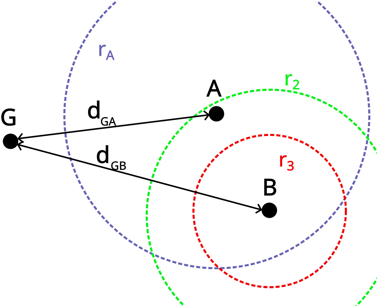
Figure 2. Schematic of two nodes with different ranges illustrated by the dotted circles. If $r_B=r_2$, $A$ and $B$ regard each other as neighbors and the farthest from the barycenter $G$ is marked as connected (given that it is not already marked).

2.1 Optimized Relay Placement for one heterogeneous link (ORPHe)

A method for placing one or multiple relays with a fixed communication range $r$ between two nodes, $A$ and $B$ with possibly different respective ranges $r_A$ and $r_B$ will be described in the following. The pseudocode is displayed in Algorithm 1.

The goal is to have a balanced placement. This means that the distance between each successive node is treated in the same way. To do so, we first consider the maximum distance between two successive nodes. It will be equal to the smaller of their ranges. This distance will be reduced by a positive real factor less than or equal to one that depends only on (a) the distance between $A$ and $B$, and (b) on the values of the ranges $r$, $r_A$ and $r_B$. Thus, this factor is common to all links between $A$ and $B$. This approach prevents a link from becoming weak while another one may afford to lose some strength.

In the following, the distance between two points $P_1$ and $P_2$ will be denoted $d(P_1,P_2)$. Because it is a recurring value, the distance between $A$ and $B$ will be treated as an exception and referred to as $AB$.

A method for the case where $r_A=r_B\le r$ is proposed in Lloyd and Xue (2007), whereas a generalization with no restrictions on the ranges, except that they are positive is proposed in Han et al. (2010). The latter defines $r_A^{\prime }=min(r_A,r)$, $r_B^{\prime }=min(r_B,r)$. It also defines $n$, the number of relays. $n=0$ if $A$ and $B$ are in range, i.e., $AB\le min(r_A^{\prime },r_B^{\prime })$, and $n=⌈\frac{AB-r_A^{\prime }-r_B^{\prime }}{r}⌉+1$ otherwise. If $n=1$, place the relay at $r_A^{\prime }=min(r_A,r)$ from $A$ towards $B$. If $n\ge 2$, after placing the first relay near $A$, place a second at $r_B^{\prime }=min(r_B,r)$ from $B$ towards $A$. The remaining $n-2$ relays should be evenly distributed between the first and second relays.

Even if it is sufficient to provide the connection between $A$ and $B$, some links may be under strain, while the others have room to spare. For example, if $r_A\le r$, the relay next to $A$ will be as far from $A$ as it can be, while if $\frac{AB-r_A^{\prime }-r_B^{\prime }}{r}\ne ⌈\frac{AB-r_A^{\prime }-r_B^{\prime }}{r}⌉$ the distance between the relays will be less than $r$.

For our method, and similarly to Han et al. (2010), we define $r_A^{\prime }=min(r_A,r)$ and $r_B^{\prime }=min(r_B,r)$, then the required number of relays is computed with $n=⌈\frac{AB-r_A^{\prime }-r_B^{\prime }}{r}⌉+1$. If $n\ge 1$, the factor is defined as $k=\frac{1}{r_A^{\prime }+(n-1)r+r_B^{\prime }}$. The position of the relays starting from $A$ are given by

$\left\{\begin{array}{cc}{x}_j\hfill & =x_{j-1}+k{r}_{j-1}\mathrm{\Delta }x,\hfill \\ y_j\hfill & =y_{j-1}+k{r}_{j-1}\mathrm{\Delta }y,\hfill \end{array}\right.(1)$

with $j\in \{1,\dots ,n\}$ and $\mathrm{\Delta }x=x_B-x_A$, $\mathrm{\Delta }y=y_B-y_A$. Here $x_0=x_A$, $y_0=y_A$, $r_0=r_A^{\prime }$. For other values of the indices, $x_j$, $y_j$ and $r_j$ (with $j\ne 1$) are the coordinates and the range of the $j^{th}$ relay counting from node $A$. The relays are assumed to have the same range $r$, thus $r_j=r,\forall j\ne 0$. A scenario with two relays is illustrated in Figure 3.

Figure 3

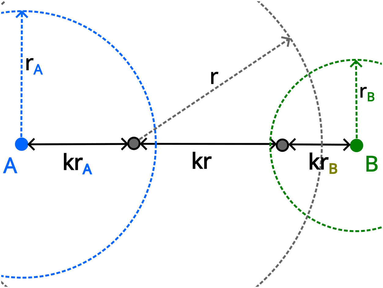
Figure 3. RN (in grey) placement between two INs with different ranges (blue and green) with the ORPHe method. The distance between two nodes is the maximal distance, given by $r$, $r_A$ or $r_B$, reduced by a common factor $k\le 1$.

Equation 1 provides us with an iterative way of positioning RNs to increase Signal-to-Noise Ratio (SNR) across all links, instead of just those between the RNs.

In Algorithm 1, this method is used to realign a set of nodes, or a segment, $\mathcal{S}$. Its first and last nodes, $S_{\mathit{first}}$ and $S_{\mathit{last}}$ respectively, are the ones that will play the role of $A$ and $B$. This algorithm returns the new segment ${\mathcal{S}}_{\mathit{new}}$ with new elements, except for the first and the last.

2.2 The BRHEN approach

In this section, the concept of segment associated with an IN is used. It refers to the set which includes the IN and all of the relays that are successively placed starting from that node. Two segments will be considered neighbors if at least one node from the first segment is a neighbor of at least one node from the second segment.

The proposed BRHEN approach is a heuristic method for heterogeneous networks that aims to connect all INs using the minimum number of relays. After a first initialization, BRHEN operates in rounds. A round begins with a search for neighbors, followed by a relocation of the current relays to improve link stability if a neighbor is found. If the segment is not connected, the round concludes with the placement of a new relay. Only when the last two unconnected segments see each other as neighbors does the algorithm exit the loop and returns the complete set of nodes. For reference, the pseudocode is displayed in Algorithm 2.

In the Following, the details of these steps will be unfolded. The set of INs will be referred to as $\mathcal{I}\mathcal{N}$ and each IN is associated to a index $i\in \{0,\dots ,N-1\}$, with $N=|\mathcal{I}\mathcal{N}|$, the number of INs. Figure 4 provides a visual example with 7 INs. The INs all have a range of 200 m, with the exception of $I{N}_5$, which has a range of 100 m. The RNs have a range of 300 m. A color is assigned to each $i$.

Figure 4

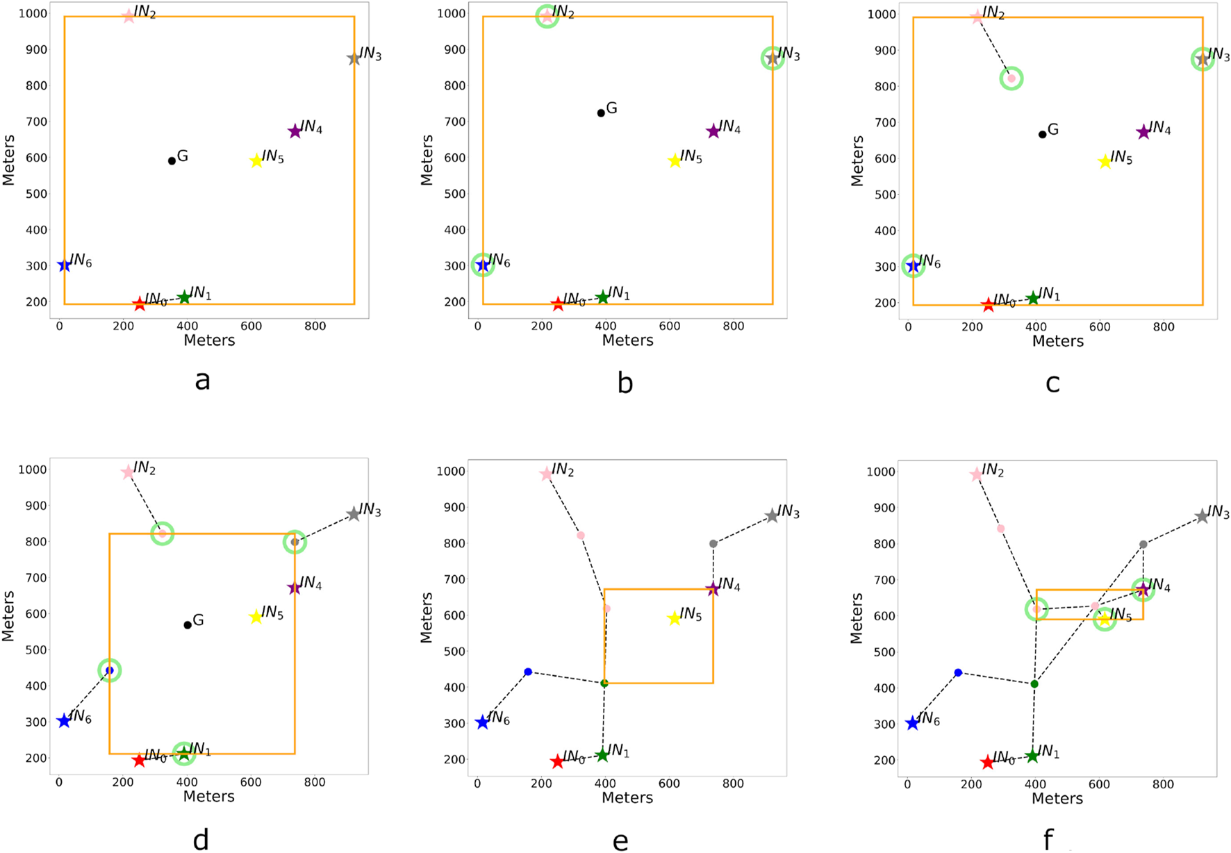
Figure 4. Some steps of the BRHEN algorithm are given above. The dashed lines represent the possibility of connection. And the side of the orange rectangle highlights the considered nodes for relay placement (a) Initialization phase: defining the first BNs. $I{N}_0$ sees $I{N}_1$ as a neighbor, the farthest from $G$ $(I{N}_0)$ is marked as connected. (b) Circled in green: the eligible nodes after discarding the connected one. (c) First relay placement: there are now two elements in ${\mathcal{S}}_2$. This relay replaces $I{N}_2$ in ${\mathcal{L}}_2$ becoming the eligible node for ${\mathcal{S}}_2$. (d) Start of the second round. (e) Start of round 3, only the segments 1, 2 and 4 are not connected, but 1 will be marked as connected before 2 places the last relay necessary for the network to be complete (f) Shows the final outcome. ${\mathcal{S}}_2$ has been rearranged by the ORPHe algorithm between its first and third element.

Algorithm 1

Algorithm 1.ORPHe.

2.2.1 Initialization

BRHEN assigns a segment with the corresponding index to each initial node, i.e., the segment $i$ is the set with the initial node $i$ and all the relays that are successively placed starting from that node. The elements of the segment $i$ will be ordered with the initial node being the first and the most recently added relay being the last—if no relay has been added yet, the initial node is also the last.

The information of the set of $\mathcal{I}\mathcal{N}$ is copied into three different sets at the beginning of the algorithm, each with a different function. $\mathcal{L}$ is the set of the last node or relay from each segment, its elements will be substituted with the newly added relays for the corresponding segment during the round. For each segment: $\mathcal{S}$ records the entire segment from its initial node to the last relay placed and $\bar{\mathcal{S}}$ holds the part of the segment from its last element that had a neighbor to its last element—until a neighbor is found, it is the same as $\mathcal{S}$. $\mathcal{C}$ represents the set of the segments that are connected. Each time two segments become neighbors, only one will be added to $\mathcal{C}$. The loop can now start and run until all the segments are connected, i.e., until $|\mathcal{C}|=N-1$.

Before using an example for a better understanding of the algorithm, let us first detail some of its key steps.

Algorithm 2

Algorithm 2.BRHEN.

2.2.2 Key steps

2.2.2.1 Remark

During a round of the BRHEN algorithm, different segments will in turn be the focus as the index $i$ will vary. When a segment is the focus, its last element, ${\mathcal{L}}_i\equiv (x_i,y_i,r_i)$, is the true focus. It will be referred to as the considered node in the details of the key steps.

2.2.2.2 Border nodes (BNs) identification

The Border Nodes (BNs) are selected from the nodes that were not previously BNs and belong to an unconnected segment. Within this set of nodes, those having coordinates corresponding to at least one extremum ($x_{\mathit{min}}$, $x_{\mathit{max}}$, $y_{\mathit{min}}$, $y_{\mathit{max}}$) become the BNs. This selection is done inside the function $\mathrm{b}\mathrm{o}\mathrm{r}\mathrm{d}\mathrm{e}\mathrm{r}\mathrm{s}$ which takes $\mathcal{L}$ and $\mathcal{C}$ as variables and gives back the indices of the elements of $\mathcal{L}$ that constitute the BNs.

2.2.2.3 Barycenter

The BRHEN algorithm uses the (unweighted) barycenter of the eligible nodes to provide a direction towards which the RNs will be placed and to use as reference for selecting the connected segment when necessary. The eligible nodes for the barycenter computation will always be part of $\mathcal{L}$. We define a function $\mathrm{B}\mathrm{a}\mathrm{r}\mathrm{y}\mathrm{c}\mathrm{e}\mathrm{n}\mathrm{t}\mathrm{e}\mathrm{r}$ which takes as input the set of the indices $k$ of the elements of $\mathcal{L}$ to be considered and outputs the point $G\equiv (x_G,y_G)$ using the following formulae for the coordinates:

$\left\{\begin{array}{cc}{x}_G\hfill & =\frac{1}{N_k}{\displaystyle \sum _k}{x}_k,\hfill \\ y_G\hfill & =\frac{1}{N_k}{\displaystyle \sum _k}{y}_k,\hfill \end{array}\right.(2)$

with the sums spanning all the elements to be considered and $N_k$ denoting the number of elements.

2.2.2.4 Finding the neighbors

To determine if a segment is connected to the currently considered segment, ${\mathcal{S}}_i$, a search for neighbors of ${\mathcal{L}}_i$ is initiated. A node $B$ (with range $r_B$) from a different segment ${\mathcal{S}}_j$ and the considered node are neighbors if the distance between them is less than the smallest range of the two nodes $(d({\mathcal{L}}_i,B)\le min(r_i,r_B))$ — see Figure 2 where $A={\mathcal{L}}_i$. Because there is no a priori knowledge about which element of ${\mathcal{S}}_j{\mathcal{L}}_i$ is the closest, this evaluation is done for each element of ${\mathcal{S}}_j$. One neighbor is sufficient for the two segments to be connected.

The function that checks for a neighbor in another segment is called $\mathrm{N}\mathrm{e}\mathrm{i}\mathrm{g}\mathrm{h}\mathrm{b}\mathrm{o}\mathrm{r}$ in the pseudo-code. It takes as input the considered node and a segment and returns $\mathrm{T}\mathrm{r}\mathrm{u}\mathrm{e}$ if there is a neighbor or $\mathrm{F}\mathrm{a}\mathrm{l}\mathrm{s}\mathrm{e}$ otherwise. This function has to be applied to all the segments ${\mathcal{S}}_j$ with $j\ne i$ for the search to be complete. If two segments are neighbors, one of them (${\mathcal{S}}_j$ or ${\mathcal{S}}_i$) will be marked as connected.

2.2.2.5 Choosing which segment to mark as connected

The simplest approach to determine which segment is marked as connected is to consistently mark the same segment, either the one identified by $i$ or the one identified by $j$. Nonetheless, an indicator that it is converging is that each new relay gets closer to $G$. The closer we get to $G$ in one step, the faster it converges. Applying the simplest approach fails to guarantee that the segment that remains unconnected is the nearest one to $G$ (whether it is $i$ or $j$). With this in mind, a more elaborate selection strategy has been implemented. There are two cases.

The first one occurs when ${\mathcal{L}}_i$ is closer to $G$ than the last element of ${\mathcal{S}}_j$, ${\mathcal{L}}_j$ and that the segment $j$ has not yet been marked as connected. If the two conditions are met, $j$ is added to $\mathcal{C}$ and is, from now on, marked as connected. The second case occurs when ${\mathcal{L}}_j$ is closer to $G$ than ${\mathcal{L}}_i$. In this situation, ${\mathcal{S}}_i$ is marked as connected and added to $\mathcal{C}$ (see Figure 2). We now have $i\in \mathcal{C}$ and this segment cannot be considered for marking other neighbor segments as connected nor for placing RNs.

This strategy provides a way to keep the closest segment to $G$, thus moving more effectively towards the other segments. Since two nodes do not mark each other as neighbors, this approach will prevent all segments from being marked as connected while the network is not yet connected (before a path from each node to all the others is available). This method will end with the two last segments meeting each other and one remaining out of $\mathcal{C}$. Thus, the end of the loop is reached when $|\mathcal{C}|=N-1$.

2.2.2.6 Realignment of the current segment

This part is optional, although it is implemented in order to reduce the distance between the nodes. Using the placement method for one heterogeneous link described above, it is ensured that all the distances between the nodes of the current segment ${\bar{\mathcal{S}}}_i$ are less than the maximum range by a positive factor $\le 1$.

Here is an example to illustrate how this realignment works in the algorithm. Let ${\mathcal{S}}_i=\{A,B,C,D,E,F\}$ and ${\bar{\mathcal{S}}}_i=\{C,D,E,F\}$. Inputting ${\bar{\mathcal{S}}}_i$ in the ORPHe algorithm (with the range for the RNs), the algorithm will output a better positioning for the RNs as ${\bar{\mathcal{S}}}_i=\{C,D^{\prime },E^{\prime },F\}$, with $D^{\prime }$ and $E^{\prime }$ being new positions. Then the new positions are substituted to the previous ones in ${\mathcal{S}}_i$ which is now $\{A,B,C,D^{\prime },E^{\prime },F\}$. Finally, ${\bar{\mathcal{S}}}_i$ is reinitialized to contain only the last element of ${\mathcal{S}}_i$, ${\bar{\mathcal{S}}}_i=\{F\}$. The set ${\bar{\mathcal{S}}}_i$ must contain at least three elements for that process to take place.

The function called $\mathrm{R}\mathrm{e}\mathrm{a}\mathrm{l}\mathrm{i}\mathrm{g}\mathrm{n}$ in the pseudo-code performs this task. The function takes ${\mathcal{S}}_i$ and ${\bar{\mathcal{S}}}_i$ as inputs, changes the elements in ${\mathcal{S}}_i$ and reinitializes ${\bar{\mathcal{S}}}_i$ as described above.

A similar realignment can be performed on the current segment ${\bar{\mathcal{S}}}_j$ but it is more tedious because the neighbor node may not be the last element of ${\bar{\mathcal{S}}}_j$. Therefore, the realignment can only be done from the first element of ${\bar{\mathcal{S}}}_j$ to the neighbor element. The function that takes into account this information is called $\mathrm{R}\mathrm{e}\mathrm{a}\mathrm{l}\mathrm{i}\mathrm{g}{\mathrm{n}}^{*}$.

2.2.2.7 RN placement

The BRHEN algorithm determines the RN placement direction based on the position of the barycenter of the eligible nodes. The eligible nodes are the ${\mathcal{L}}_k$ with $k\in \mathcal{I}\mathcal{D}$ which were not marked as connected during the round—i.e., $k\in \mathcal{I}\mathcal{D}\backslash (\mathcal{I}\mathcal{D}\cap \mathcal{C})$. There is the possibility that this set now contains only the index of the considered segment. In that case, the positioning of a new RN is bypassed since the barycenter is at the same position as the considered node rendering the concept of direction towards the barycenter void.

If the distance between the considered node and the barycenter $G$ is greater than the smaller range between that of $A$ and that of a RN—i.e., if $d=d({\mathcal{L}}_i,G)<r_{\mathit{min}}=min(r_i,r)$ — the RN is placed at a distance corresponding to $r_{\mathit{min}}$ towards $G$, using the following formulae for the coordinates:

$\left\{\begin{array}{cc}x\hfill & =x_i+\frac{r_{\mathit{min}}}{d}\left(x_G-x_i\right),\hfill \\ y\hfill & =y_i+\frac{r_{\mathit{min}}}{d}\left(y_G-y_i\right).\hfill \end{array}\right.(3)$

Otherwise, if $d\le r_{\mathit{min}}$ the RN is placed at the barycenter with $x=x_G$ and $y=y_G$. The new nodes $(x,y,r)$ will replace the current element ${\mathcal{L}}_i$ and will be added to ${\mathcal{S}}_i$ and ${\bar{\mathcal{S}}}_i$ as their last element.

2.2.3 Detailed workings with example

This description of the workings of the BRHEN algorithm uses the scenario presented in Figure 4 as reference.

2.2.3.1 First round

The round starts by identifying the BNs with the $\mathrm{B}\mathrm{o}\mathrm{r}\mathrm{d}\mathrm{e}\mathrm{r}\mathrm{s}$ function. Since it is the first time, $\mathcal{L}$ is the set of initial nodes and $\mathcal{C}$ is empty. The function thus considers all the INs and its output, the set $\mathcal{I}\mathcal{D}$, contains the indices of the INs which are BNs. This set is $\{\mathrm{0,2,3,6}\}$ and it is used to compute a first barycenter $G$. Figure 4a shows in orange the rectangle defined by the BNs and which encloses all the other yet unconsidered nodes.

Beginning with the index 0, the search for neighbors of ${\mathcal{L}}_0=I{N}_0$ is initiated and one is found in $I{N}_1$. The segment of the farthest node from $G$ is marked as connected and $\mathcal{C}=\{0\}$. Now that the considered segment is marked as connected, it is no longer eligible for RN placement and will not be considered for future barycenter computations. The connection between the two nodes is represented by a dashed line joining them in Figure 4.

The next segment is now considered with the index 2, ${\mathcal{L}}_2=I{N}_2$ has no neighbors and is eligible for a RN placement. The barycenter of all eligible nodes ($I{N}_2$, $I{N}_3$, $I{N}_6$, circled in green in Figure 4b) is computed, and a RN is placed in that direction at a distance $min(r_2,r)$ from $I{N}_2$ (see Figure 4c). This new node becomes the new ${\mathcal{L}}_2$, making it the eligible element of the second segment for the next barycenter computations. In turn, segments 3 and 6 go through the same process, finding no neighbors and placing a RN each.

2.2.3.2 Subsequent rounds

The second round starts with a connected segment and three new nodes as illustrated in Figure 4d. The new BNs are circled in green. $I{N}_4$ is not one of them, as it is slightly inside the orange rectangle. In this round, ${\mathcal{L}}_1=I{N}_1$ will place a RN after finding no other neighbor than $I{N}_0$, and so will ${\mathcal{L}}_2$. ${\mathcal{L}}_3$ will connect with $I{N}_4$ and as the former will be farther from the barycenter ${\mathcal{S}}_3$ will be marked as connected. Similarly for ${\mathcal{L}}_6$, it will connect with the new ${\mathcal{L}}_1$ and its segment will be marked as connected. Thus, by the end of the second round $\mathcal{C}=\{\mathrm{0,3,6}\}$ and the third round will start with the structure shown in Figure 4e.

In the third round, only ${\mathcal{L}}_1$ and ${\mathcal{L}}_4=I{N}_4$ will be considered first. However, ${\mathcal{L}}_1$ will see ${\mathcal{L}}_2$ as a neighbor and its segment will be marked as connected leaving ${\mathcal{L}}_4$ alone. The realignment functions are applied to both ${\mathcal{S}}_1$ and ${\mathcal{S}}_2$, but only ${\bar{\mathcal{S}}}_2$ has enough elements for the functions to modify its content. The realignment can be seen by comparing Figures 4e, f. ${\mathcal{L}}_4$ being alone, in this round there is no eligible node for RN placement. Furthermore, the short range of $I{N}_5$, prevents $I{N}_4$ from connecting with it.

The fourth round starts with the same set of $\mathcal{L}$ as the previous one, but with ${\mathcal{S}}_1$ being connected, the BNs and the eligible nodes are different. ${\mathcal{L}}_2$ will place the final RN on the barycenter because $d({\mathcal{L}}_2,G)<r_{\mathit{min}}$ and all other eligible nodes will see it as neighbor. In its turn, ${\mathcal{L}}_5$ will be marked as connected as it finds ${\mathcal{L}}_2$ as neighbor and closer to $G$. The set of connected segments is now $\mathcal{C}=\{\mathrm{0,1,3,4,5,6}\}$. Therefore, the condition of $|\mathcal{C}|=N-1$ is met, and the algorithm returns the set containing all the nodes in the network.

2.3 Algorithms analysis

In this subsection, original proofs for the validity of the formulae used in the ORPHe algorithm and the convergence of BRHEN algorithm are given.

2.3.1 Analysis of ORPHe

Property 2.3. The coordinates of a point $P\equiv (x,y)$ on the line between two different points $A\equiv (x_A,y_A)$ and $B\equiv (x_B,y_B)$, at the distance $r\ge 0$ from $A$ and in the direction of $B$, are given by

$\left\{\begin{array}{cc}x\hfill & =x_A+\frac{1}{AB}r\mathrm{\Delta }x,\hfill \\ y\hfill & =y_A+\frac{1}{AB}r\mathrm{\Delta }y,\hfill \end{array}\right.(4)$

with $\mathrm{\Delta }x=x_B-x_A$ and $\mathrm{\Delta }y=y_B-y_A$. Therefore, the relation between the $x$ $(y)$ coordinates of $A$ and $P$ is provided by a term composed of (a) the ratio between the distance $r$ and the distance between $A$ and $B$ and (b) the difference between their coordinates $\mathrm{\Delta }x$ $(\mathrm{\Delta }y)$.

Proposition 2.4. If $r_A$ and $r_B\in {\mathbb{R}}^{+}$ and both are not equal to zero, there is a real factor $m>0$ such that there is a point $P=(x,y)$ on the line defined by $A$ and $B$ — two different points — which is at a distance $m{r}_A$ and $m{r}_B$ from $A$ and $B$, respectively. Its coordinates are given by

$\left\{\begin{array}{cc}x\hfill & =x_A+k{r}_A\mathrm{\Delta }x,\hfill \\ y\hfill & =y_A+k{r}_A\mathrm{\Delta }y,\hfill \end{array}\right.(5)$

$\mathrm{w}\mathrm{i}\mathrm{t}\mathrm{h}k=\frac{1}{AB}m=\frac{1}{AB}\left(\frac{AB}{r_A+r_B}\right)=\frac{1}{r_A+r_B}.(6)$

$m$ is unique and equal to $\frac{AB}{r_A+r_B}$ and the position of $P$ is determined by substituting $AB$ with the sum of the ranges in Equation 4. This allows us to find a point that reduces (or extends) both distances $r_A$ and $r_B$ by the same factor.

Proof. The proof will be done only for the $x$ coordinate, as it is similar for the $y$ coordinate. Equating the result from Property 2.3 for a point on the line defined by $A$ and $B$ at a distance $m{r}_A$ from $A$ with its result for a point on the same line at a distance $m{r}_B$ from $B$, yields

$\begin{array}{ccc}\hfill & \hfill x_A+\frac{1}{AB}m{r}_A\mathrm{\Delta }x=& x_B+\frac{1}{AB}m{r}_B\left(-\mathrm{\Delta }x\right)\hfill \\ \iff \hfill & \hfill \frac{1}{AB}m{r}_A\mathrm{\Delta }x=& \left(1-\frac{1}{AB}m{r}_B\right)\mathrm{\Delta }x\hfill \\ \iff \hfill & \hfill \frac{1}{AB}m{r}_A=& 1-\frac{1}{AB}m{r}_B\hfill \\ \iff \hfill & \hfill m=& \frac{AB}{r_A+r_B}.\hfill \end{array}$

Thus, the $x$ coordinate of the point $P$ is given by

$x=x_A+\frac{1}{AB}m{r}_A\mathrm{\Delta }x=x_A+k{r}_A\mathrm{\Delta }x,$

with $k=\frac{1}{AB}m=\frac{1}{r_A+r_B}$.

Remark 2.5. In the following, we will consider the connectivity of the nodes. Since all relays will have the same range $r$ and the initial nodes $A$ and $B$ may have distinct ranges, for the connectivity between an initial node and a relay, we must consider the smaller range as the maximum distance between the two. Thus, from now on, $r_A$ and $r_B$ will be by default $min(r_A,r)$ and $min(r_B,r)$, respectively.

Proposition 2.6. Let $A$ and $B$ be two unconnected nodes with ranges $r_A$ and $r_B$, respectively. The minimum number of additional nodes with range $r>0$ for $A$ and $B$ to be connected is given by

$n=⌈\frac{AB-\left(r_A+r_B\right)}{r}⌉+1.(7)$

Where $AB$ is the distance between the two unconnected nodes, $r_A$ and $r_B$ are the ranges considered for these nodes (see Remark 2.5), while $r$ is the range of the additional nodes.

Proof. After placing a node towards $B$ at a distance of $r_A$ from $A$ and a node towards $A$ at a distance of $r_B$ from $B$, the remaining distance between those two relays is $AB-(r_A+r_B)$. The minimum number of segments of length $r$ needed to cover that distance is $n_r=⌈\frac{AB-(r_A+r_B)}{r}⌉-1$. Finally, the first two relays are added to obtain the total number of relays: $n=⌈\frac{AB-(r_A+r_B)}{r}⌉+1$.

Theorem 2.7. Let $A$ and $B$ be two unconnected nodes with respective ranges $r_A$ and $r_B$ and $n\in {\mathbb{N}}^{+}$ be the number of additional nodes. Let us assign an index $j$ to each additional node that will be placed between $A$ and $B$ starting from $A$. Thus, $j=1$ and $j=n$ refer to the closest to $A$ and the closest to $B$, respectively. For any number of nodes, $n\in {\mathbb{N}}^{+}$, with range $r$ to be placed in between $A$ and $B$, the coordinates of the node $j\in \{1,\dots ,n\}$, are given by

$\left\{\begin{array}{cc}{x}_j\hfill & =x_A+k\mathrm{\Delta }x\left(r_A+\left(j-1\right)r\right),\hfill \\ y_j\hfill & =y_A+k\mathrm{\Delta }y\left(r_A+\left(j-1\right)r\right),\hfill \end{array}\right.(8)$

$\mathrm{w}\mathrm{i}\mathrm{t}\mathrm{h}k=\frac{1}{r_A+\left(n-1\right)r+r_B}.$

The coordinates can also be expressed using the coordinates of the previous node:

$\left\{\begin{array}{cc}{x}_j\hfill & =x_{j-1}+k{r}_{j-1}\mathrm{\Delta }x,\hfill \\ y_j\hfill & =y_{j-1}+k{r}_{j-1}\mathrm{\Delta }y,\hfill \end{array}\right.(9)$

with $x_0=x_A$, $r_0=r_A$ and $r_j=r$ for $j>0$.

Furthermore, all nodes are connected for $n\ge ⌈\frac{AB-(r_A+r_B)}{r}⌉+1$.

Equation 8 give the positions of all the RNs from the position of one of the INs depending on its index, whereas Equation 9 are the iterative formulae that give the position of the subsequent RNs from the previous one (or from the IN for the first RN).

Proof. Firstly, the placement of the $j$^th relay from $A$ towards $B$ can be thought of as the placement of the only relay between $A$ and $B$ with new respective ranges defined as $r_A^{\prime }=r_A+(j-1)r$ and $r_B^{\prime }=r_B+(n-j)r$. The definition of $k$ from Proposition 2.4 is

$\begin{array}{ll}\hfill k& =\frac{1}{r_A^{\prime }+r_B^{\prime }}\hfill \\ \hfill & =\frac{1}{r_A+\left(n-1\right)r+r_B}.\hfill \end{array}$

Then, with Equation 5 we can express the coordinates of the node $j$ — shown only for the $x$ coordinate as it is similar for the $y$ — as $x_i=x_A+k\mathrm{\Delta }(r_A+(j-1)r)$.

$\begin{array}{ll}\hfill x_j& =x_A+k\mathrm{\Delta }x\left(r_A+\left(j-1\right)r\right)\hfill \\ \hfill & =\underset{x_{j-1}}{\underbrace{x_A+k\mathrm{\Delta }x\left(r_A+\left(j-2\right)r\right)}}+\hspace{0.17em}kr\mathrm{\Delta }x\hfill \\ \hfill & =x_{j-1}+kr\mathrm{\Delta }x,\hfill \end{array}$

with $x_0=x_A$, $r_0=r_A$ and $r_j=r$ for $j>0$. Secondly, with $n$ from Equation 7, the distance between two consecutive nodes $j-1$ and $j$ for $j\in \{1,\dots ,n\}$, is given by

$\begin{array}{ll}\hfill d& =\sqrt{{\left(k{r}_{j-1}\mathrm{\Delta }x\right)}^2+{\left(k{r}_{j-1}\mathrm{\Delta }y\right)}^2}\hfill \\ \hfill & =k{r}_{j-1}\underset{AB}{\underbrace{\sqrt{\mathrm{\Delta }{x}^2+\mathrm{\Delta }{y}^2}}}\hfill \\ \hfill & =r_{j-1}\left(\frac{AB}{r_A+\left(n-1\right)r+r_B}\right)\hfill \\ \hfill & =r_{j-1}\left(\frac{AB}{r_A+⌈\frac{AB-r_A-r_B}{r}⌉r+r_B}\right)\hfill \\ \hfill & \le r_{j-1}\left(\frac{AB}{r_A+\frac{AB-r_A-r_B}{r}r+r_B}\right)\hfill \\ \hfill & =r_{j-1}.\hfill \end{array}$

Thus, the distance between the two consecutive nodes $j-1$ and $j$ is smaller than the range of $r_{j-1}$ and the connectivity is guaranteed for $n\ge ⌈\frac{AB-(r_A+r_B)}{r}⌉+1$.

Proposition 2.8. Let us consider the maximum range of each node to be the distance within which a desired channel capacity is ensured and assume two different propagation channels, one being between an IN and a RN and the other one between two RN, with possibly different Path-Loss Exponents (PLEs). Let us also assume that all the RNs have the same range. Finally that the bandwidth used by each node is the same and that we have an Additive White Gaussian Noise (AWGN). Then, the ORPHe placement method is an improvement on a method leaving some distances between nodes to be maximal and is optimal for the special case where the two PLE are identical.

Proof. For an AWGN channel the channel capacity is given by

$c=W{\log }_2\left(1+\mathrm{S}\mathrm{N}\mathrm{R}\right),$

where $W$ is the bandwidth. This capacity is a function of the SNR which is inversely proportional to $d^{\alpha }$, with $d$, the distance from the source and $\alpha$, the PLE. The range of each node is defined by the distance at which a certain $c$ is ensured and this $c$ is the same for each node. However, if the bandwidth is the same for all links, equal values of $c$ correspond to equal values of SNR. Let $\alpha$ and $\beta$ be the PLE of the RN-RN and IN-RN channels, respectively, and let $A$ and $B$ be the two INs. Then, the different SNRs can be expressed as

$SN{R}_{RN}=\frac{F}{d^{\alpha }},SN{R}_A=\frac{F_A}{d^{\beta }},SN{R}_B=\frac{F_B}{d^{\beta }},(10)$

with $F$, $F_A$ and $F_B$ taking into account the transmission power, the fading, the bandwidth, and the frequency of each node.

Since the idea behind the ranges is that they give the same capacity, substituting $d$ with the appropriate range yields

$\frac{F}{r^{\alpha }}=\frac{F_A}{r_A^{\beta }}=\frac{F_B}{r_B^{\beta }}(11)$

In our case, we have

$r_A+\left(N-1\right)r+r_B>AB$

and we want to reduce the distances between the nodes such that

$d_A+\left(N-1\right)d+d_B=AB,$

with $d_A=m_A{r}_A$, $d=mr$, $d_B=m_B{r}_B$ and $m_A$, $m$, $m_B\in \left]\mathrm{0,1}\right[$. Substituting those distances to the $r$’s in Equation 11 yields

$\frac{F}{{\left(mr\right)}^{\alpha }}=\frac{F_A}{{\left(m_A{r}_A\right)}^{\beta }}=\frac{F_B}{{\left(m_B{r}_B\right)}^{\beta }}.(12)$

However, from the last equality of Equation 11 and that of Equation 12, we get that $m_A=m_B$, leaving only $m$ and $m_A$ to be determined. The first equality of the identical equations yields $m_A=m^{\alpha /\beta }$ or $m=m_A^{\beta /\alpha }$. Thus, we have the following set of equations

$\left\{\begin{array}{c}{m}_A\left(r_A+r_B\right)+m\left(N-1\right)r=D\hfill \\ m_A=m^{\alpha /\beta }\hspace{0.17em}\text{or}\hspace{0.17em}m=m_A^{\beta /\alpha }\hfill \end{array}\right.(13)$

Let us demonstrate that, for the optimal SNR, the equalities are to be conserved when modifying the distances. If they were not, we might have, for example,

$\frac{F}{{\left(mr\right)}^{\alpha }}>\frac{F_A}{{\left(m_A{r}_A\right)}^{\beta }}.$

The channel capacity of the link between $A$ and $B$ is limited by the lowest capacity of the different hops, i.e., the right hand side. As previously, with Equation 11, we deduce that $m_A>m^{\alpha /\beta }$. This means that

$\frac{F}{{\left(m_A{r}_A\right)}^{\beta }}<\frac{F_A}{{\left(m^{\alpha /\beta }{r}_A\right)}^{\beta }}.$

Because the right-hand side is the result when assuming the equality of the SNR, we can conclude that assuming the equality is optimal.

Three different cases are to be analyzed: $\alpha =\beta$, $\alpha <\beta$ and $\alpha >\beta$.

2.3.1.1 Case $\alpha =\beta$

Equation 14 becomes $m_A=m$ and Equation 13 yields $m=\frac{AB}{(r_A+r_B)+(N-1)r}$. This is the definition of $m$ in the ORPHe algorithm, thus in the ORPHe algorithm the use of a unique coefficient $k=\frac{m}{AB}$ is the same as assuming that the PLE are the same for all links and it is the optimal placement in that case.

2.3.1.2 Case $\alpha <\beta$

Substituting $m^{\alpha /\beta }$ to $m_A$ in Equation 13, yields

$m^{\alpha /\beta }\left(r_A+r_B\right)+m\left(N-1\right)r=D.$

Given that $0<m<1$ and $\alpha /\beta <1$, we have $m^{\alpha /\beta }>m$. Then the value of the coefficient $m$, which is solution of Equation 13, will be less than that of the first case (which will be referred to as $m_0$ from now on). With this in mind, we may qualitatively compare the SNRs that would be obtained by assuming a unique PLE, with the ones that would be obtained with different PLE. For the latter, the equality on the SNR still holds. However, substituting $m_0$ to both $m$ and $m_A$ yields

$\frac{F_A}{m_0^{\beta }{r}_A^{\beta }}>\frac{F}{m_0^{\alpha }{r}^{\alpha }},(14)$

since $\beta >\alpha$. As a consequence, the SNR between the RNs will be the limiting factor for the channel capacity. On the other hand, considering the two PLE yields

$\frac{F_A}{{\left(m_A{r}_A\right)}^{\beta }}=\frac{F_A}{{\left(m^{\alpha /\beta }{r}_A\right)}^{\beta }}=\frac{F_A}{m^{\alpha }{r}_A^{\beta }}=\frac{F}{m^{\alpha }{r}^{\alpha }}.(15)$

Comparing the limiting SNR from two previous results to the limiting SNR when nothing is done (Equation 11) gives the following successive inequalities

$\frac{F}{m^{\alpha }{r}^{\alpha }}>\frac{F}{m_0^{\alpha }{r}^{\alpha }}>\frac{F}{r^{\alpha }}.(16)$

The first inequality is because $m<m_0$ and the second one because $1/m_0^{\alpha }>1$.

2.3.1.3 Case $\alpha >\beta$

Substituting $m_A^{\beta /\alpha }$ to $m$ in Equation 13 allows us to follow the same reasoning with $m_A$ as in the previous case with $m$. Here $m_A<m$, Equation 14 becomes

$\frac{F_A}{m_0^{\beta }{r}_A^{\beta }}<\frac{F}{m_0^{\alpha }{r}^{\alpha }},(17)$

since $\alpha >\beta$ and the optimal SNR is

$\frac{F_A}{m_A^{\beta }{r}_A^{\beta }}=\frac{F}{m^{\alpha }{r}^{\alpha }}=\frac{F}{{\left(m_A^{\beta /\alpha }r\right)}^{\alpha }}=\frac{F}{m_A^{\beta }{r}^{\alpha }}.(18)$

Finally, comparing the limiting SNRs yields

$\frac{F_A}{m_A^{\beta }{r}_A^{\beta }}>\frac{F_A}{m_0^{\beta }{r}_A^{\beta }}>\frac{F_A}{r_A^{\beta }}.(19)$

The first inequality is due to $m_A<m_0$ and the second one to $1/m_0^{\beta }>1$.

Thus, assuming that the channels have the same LPE for determining a coefficient to reduce the distance between the node as is implicitly done in the ORPHe algorithm, is suboptimal yet enhances, nonetheless, the channel capacity compared to leaving some distances between nodes to be maximal.

2.3.2 Analysis of BRHEN

Property 2.9. The barycenter $G\equiv (x_G,y_G)$ of $N$ points is always inside the rectangle defined by the extrema in $x$ and $y$ coordinates of those points,

$\left\{\begin{array}{cc}{x}_{\mathit{min}}\le \hfill & x_G\le x_{\mathit{max}}\hfill \\ y_{\mathit{min}}\le \hfill & y_G\le y_{\mathit{max}}.\hfill \end{array}\right.(20)$

In addition, it is equal to an extremum in $x$ or $y$ if all the points have the same $x$ or $y$ coordinate, respectively.

Proof. The proof will only be done for the $x$ coordinate, as it is similar for the $y$ coordinate. We can establish an upper bound to the value of $x_G$ by substituting all $x_j$ with $j\in \{1,\dots ,N\}$ for $x_{\mathit{max}}$ in the definition of $x_G$. It yields

$\begin{array}{ll}\hfill x_G& =\frac{{\sum }_j^N{x}_j}{N}\le \frac{N{x}_{\mathit{max}}}{N}\hfill \\ \hfill \iff x_G& \le x_{\mathit{max}}.\hfill \end{array}$

The lower bound is obtained by substituting all $x_j$ for $x_{\mathit{min}}$. It yields $x_G\ge x_{\mathit{min}}$.

It is equal if all the $x_j$ have the same value $x_j=x_{\mathit{max}}=x_{\mathit{min}}$, indicating that all the points are on a vertical line.For the $y$ coordinate, it is equal to the extrema if all the points are on a horizontal line.

This property guarantees that the new relays placed from the border nodes towards their barycenter remain within the rectangle defined by those nodes. This means that the next border identification, which only takes into account the nodes not considered yet, will have nodes strictly inside the previous rectangle to consider. As a result, the algorithm converges as the rectangles become smaller.

3 Performance evaluation

This section assesses the effectiveness of BRHEN by comparing performance across multiple metrics using simulations. The results show that BRHEN performs better in terms of the number of relays placed when the Initial Nodes (INs) are heterogeneous with respect to the communication ranges and when the relays have yet a different range. The simulations also indicate that BRHEN performs better in terms of average hop count between two INs once the network is established. Therefore, the resulting topography produces a lower data delivery latency. An analysis of the behavior of each method for large-scale networks shows that BRHEN handles large and dense networks better than its counterparts. The data also show that BRHEN is computationally light and that it is stable with regard to the positions and the number of RNs when the INs are randomly displaced by up to 10% of the smallest range. Additionally, in the last two subsections, we studied the effect of the order of consideration of the different segments on the resulting network and the effect of applying the ORPHe method within the BRHEN algorithm.

3.1 Validation simulations

The performance of BRHEN is compared to two baseline approaches. This subsection introduces the simulations setup, the performance metrics and the baseline approaches used for comparisons.

3.1.1 Simulations setup and performance metrics

The simulations consider a partitioned network with INs, with different ranges $r_{\mathit{min}}$ and $r_{\mathit{mid}}$, while the relays to be placed for network restoration have a range $r_{\mathit{max}}$ $(r_{\mathit{min}}<r_{\mathit{mid}}<r_{\mathit{max}})$. The performance is evaluated by varying the following three parameters.

• Relative communication ranges of the nodes ($r_{\mathit{min}}$, $r_{\mathit{mid}}$, $r_{\mathit{max}}$): The communication range has a great influence on the number of relays by reducing both the distance left to cover and the number of relays necessary to cover it. Here, since multiple ranges are dealt with, the performance will be assessed for (a) ranges growing with the same factor, the mutual growth coefficient $g_m$, and (b) for the two largest ranges growing relatively to the smallest ones, i.e., proportionally to the separate growth coefficient $g_s$.

• Number of Initial Nodes $N_{IN}$: The number of INs to connect is also expected to influence the number of relays to deploy.

• INs displacement $d_{IN}$: Each IN of the set is displaced in a random direction by $d_{IN}$ meters. This parameter is used to evaluate the stability of the BRHEN algorithm with respect to moving INs.

We assessed the impact of these parameters on the following eight metrics.

• Number of Relay Nodes $N_{RN}$: This is the main goal of the optimization and the clearest visualization of the performance of BRHEN.

• Average Hop count $H$: This will assess the connectivity of the resulting topology. It is calculated as the sum of the number of hops needed to connect each IN to every other through the shortest path—without counting everything twice—divided by the number of connections to make $N_{IN}(N_{IN}-1)/2$.

• Number of rounds $N_{\mathit{rounds}}$and computation time $t$: The objectives of these metrics are to show that the algorithm converges in a low number of rounds and that it is computationally light.

• Mean RN displacement $⟨d_{RN}⟩$ and Probability of $N_{RN}$ to change $\mathcal{P}[N_{RN}^{\prime }]$: These metrics are used in order to assess the stability of the BRHEN method and compare the state of the network before and after random displacements of the INs

• Difference between first and best number of RNs $\mathrm{\Delta }{N}_{RN}$: Used to visualize the improvement on the resulting $N_{RN}$ when applying the BRHEN algorithm while considering the INs and their segments in different sequences.

• Smallest SNR improvement $\mathrm{\Delta }SN{R}_{\mathit{min}}$: This metric shows the smallest improvement among the various links in a segment following realignment with the ORPHe algorithm. The parameters and the metrics are summerized in Tables 1, 2, respectively.

Table 1

Table 1. Simulation parameters.

Table 2

Table 2. Simulation metrics.

3.1.2 Baseline approaches

• CORP: This algorithm considers a homogeneous set of INs with a communication range $r$. It also assumes the RNs to have the same range. CORP is a cell-based method, and the map is divided into cells with a size corresponding to the range. The greatest distance between two adjacent cells is set to $r$. Since it corresponds to the diagonal, the dimension of the square cells is $r/\sqrt{2}$. This method operates similarly to BRHEN, as the latter’s main steps were inspired by CORP. The key distinction is in the use of cells and in the consideration of different cells for the best placement of a new RN for the CORP part. The algorithm takes in the positions of the set of INs, which must correspond to the center of a cell. To each IN corresponds an index and a segment. The first step is a search for the INs defining the rectangle which encapsulates all the INs. It will then start a loop that will continue until the set of Border Nodes (BNs) is empty. In a second loop, for each BN, it first searches the adjacent cells of each BN for neighbors. If one of a different segment is found, one of the two segments is marked as connected and will not be considered hereafter. If the number of RNs in the marked segment is greater than the number of RNs necessary for connecting its IN and its last RN in a straight line, the segment is pruned—i.e., the RNs are placed in the straight line and equidistant from each other. The second step is to evaluate each adjacent cell as a possible position for a new RN. This is done by calculating the sum of the distances between the considered cell and the other BNs. When it is done for all the BNs, the algorithm starts again from the search for the new BNs in the set including all the nodes except the ones already considered.

• MST-1tRN (enhanced): The basic idea behind this algorithm is to compute a MST and populate the edges of the MST with the required number of RNs. The MST yields a set of edges connecting the nodes such that there is a path from each node to the others with the minimum total length. In Lloyd and Xue (2007), it is assumed that all nodes have the same range $r$ and the relays have a range $r^{\prime }>r$. Thus, it does not support a heterogeneous set of INs. This is easily alleviated by applying the ORPHe method for populating the edges. This enhanced version will be our baseline approach as an algorithm that can manage a heterogeneous network.

To ensure that all methods worked under the same initial conditions in the following simulations, cells were used to place the INs. In addition, since CORP works with a unique range, this range must be the smallest; otherwise, some nodes in neighboring cells would not be connected. This is the reason why the size of a cell is defined by $r_{\mathit{min}}$.

3.2 Comparison of the different methods

In order to test the BRHEN method in a more general way, the scenarios are randomly generated. The INs are placed one by one with a random selection of a unused cell in a square area with a given side length (in number of cells). Each IN is randomly assigned a range $r_{\mathit{min}}$ (1 cell diagonal) or $r_{\mathit{mid}}$ which is greater by a given factor and the relays have the greatest range $r_{\mathit{max}}$. The factors for $r_{\mathit{mid}}$ and $r_{\mathit{max}}$ are 1.5 and 2, respectively, except for the tests where the factors are the variable parameters. For each value of the variable parameters, 1,000 random scenarios are generated, and the statistical results are the focus of the analysis. $r_{\mathit{max}}$ is assigned to the RNs because we assume that they are Unmanned Aerial Vehicles (UAVs) using their ability to be swiftly deployed anywhere. The establishment of a Line of Sight (LOS) between each other justifies their greater range.

The $N_{RN}$ and the $H$ metrics are first evaluated with increasing ranges—which is equivalent to a decreasing number of cells covering the area. Thus, we decrease the side length of the square area from 16 cells to 9 cells, which corresponds to a 78 per cent increase in range, or a growth coefficient $g_m=1.78$. It is evaluated for a fixed 7 INs. The second evaluation on those metrics is done with the same number of INs and a side of 12 cells, but the factors between $r_{\mathit{min}}$ and the other ranges ($r_{\mathit{mid}}$, $r_{\mathit{max}}$) increase. The values are given by $r_{\mathit{max}}=g_s{r}_{\mathit{min}}$ and $r_{\mathit{mid}}=\frac{g_s+1}{2}{r}_{\mathit{min}}$, where $g_s$ takes the values from 2 to 9 by increments of one. The third test on those metrics is when the side is fixed to 12 cells. The factors are also fixed to 1.5 and 2, and the number of INs increases by one from 5 to 12. The last metric is the number of rounds done in BRHEN for the network to be connected. It is evaluated for 7, 8 and 9 INs with increasing ranges as the number of cells decreases from 16 to 9.

In the following results, displayed in Figures 5–10, it should be noted that the great variance in the results is due, to a large extent, to the fact that the scenarios are generated completely randomly. This randomness means that all the INs might be placed as a cluster somewhere in the map or very disparate. Alternatively, every INs could have the smaller (or larger) range. This would influence, for example, the number of RNs of all the methods in a similar way.

Figure 5

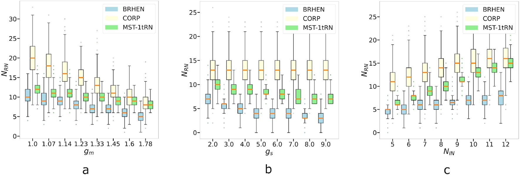
Figure 5. Results comparison regarding the evolution of the number of relays $N_{RN}$ in function of (a) the growth of all the ranges with respect to the size of the map, with $r_{\mathit{mid}}=1.5r_{\mathit{min}}$ and $r_{\mathit{max}}=2r_{\mathit{min}}$. (b) The growth of the difference between the ranges, represented by the increase of the ratio $r_{\mathit{max}}/r_{\mathit{min}}$, and (c) the number of initial nodes (INs).

Figure 6

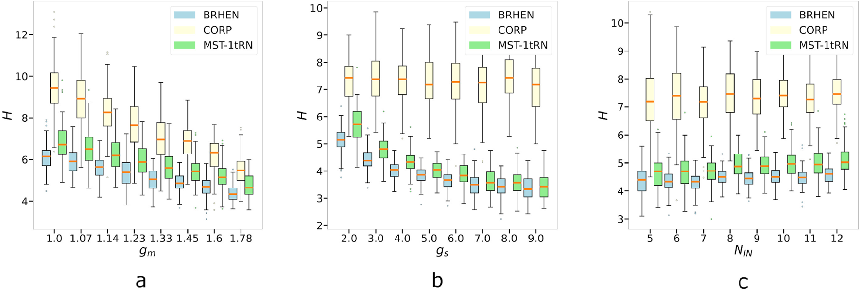
Figure 6. Results comparison regarding the evolution of the average hop count $H$ in function of (a) the growth of all the ranges with respect to the size of the map, with $r_{\mathit{mid}}=1.5r_{\mathit{min}}$ and $r_{\mathit{max}}=2r_{\mathit{min}}$. (b) The growth of the difference between the ranges, represented by the increase of the ratio $r_{\mathit{max}}/r_{\mathit{min}}$, and (c) the number of initial nodes (INs).

Figure 7

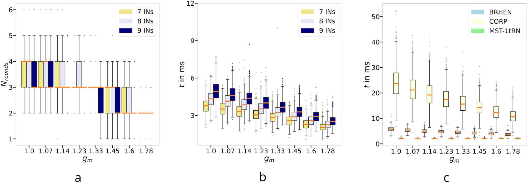
Figure 7. (a) Number of rounds in function of the range for different number of INs. (b) BRHEN computation time in milliseconds (ms) as a function of the range for different number of INs. (c) Comparison of the computing time of BRHEN (blue), CORP (yellow) and MST-1tRN (green).

Figure 8

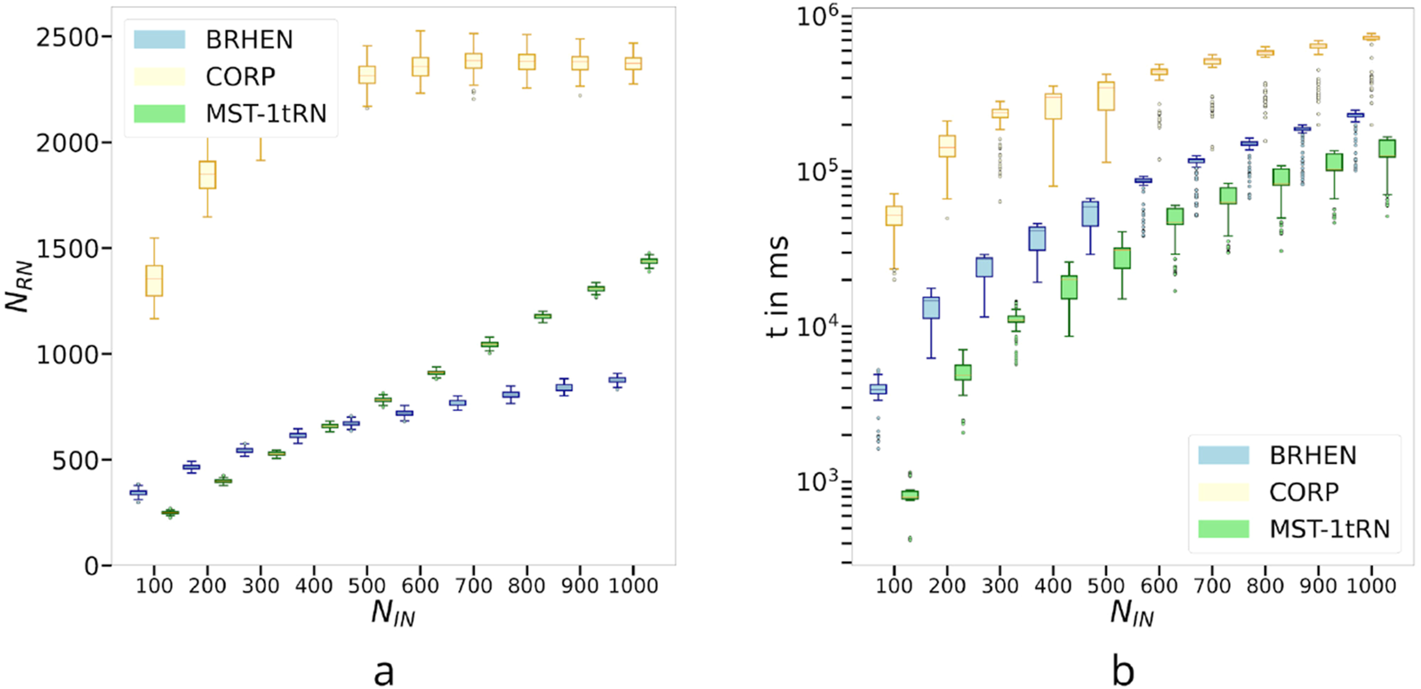
Figure 8. The large-scale behavior of the three considered methods for (a) the number of relay nodes $(N_{RN})$ placed and (b) the computation time $t$ in milliseconds.

Figure 9

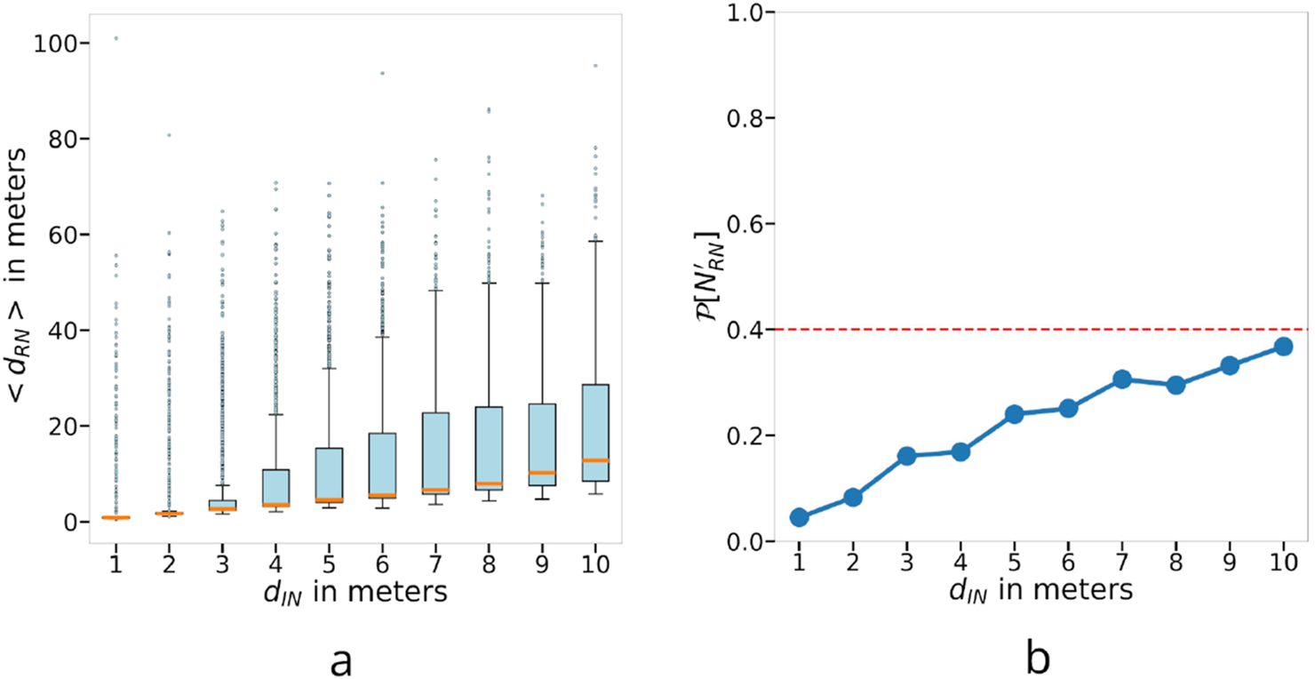
Figure 9. Assessment of the stability of the BRHEN approach. (a) Mean RN displacement in meters as a function of the distance of the IN displacements. (b) Probability that the number of RN $(N_{RN})$ changes when the INs are displaced.

Figure 10

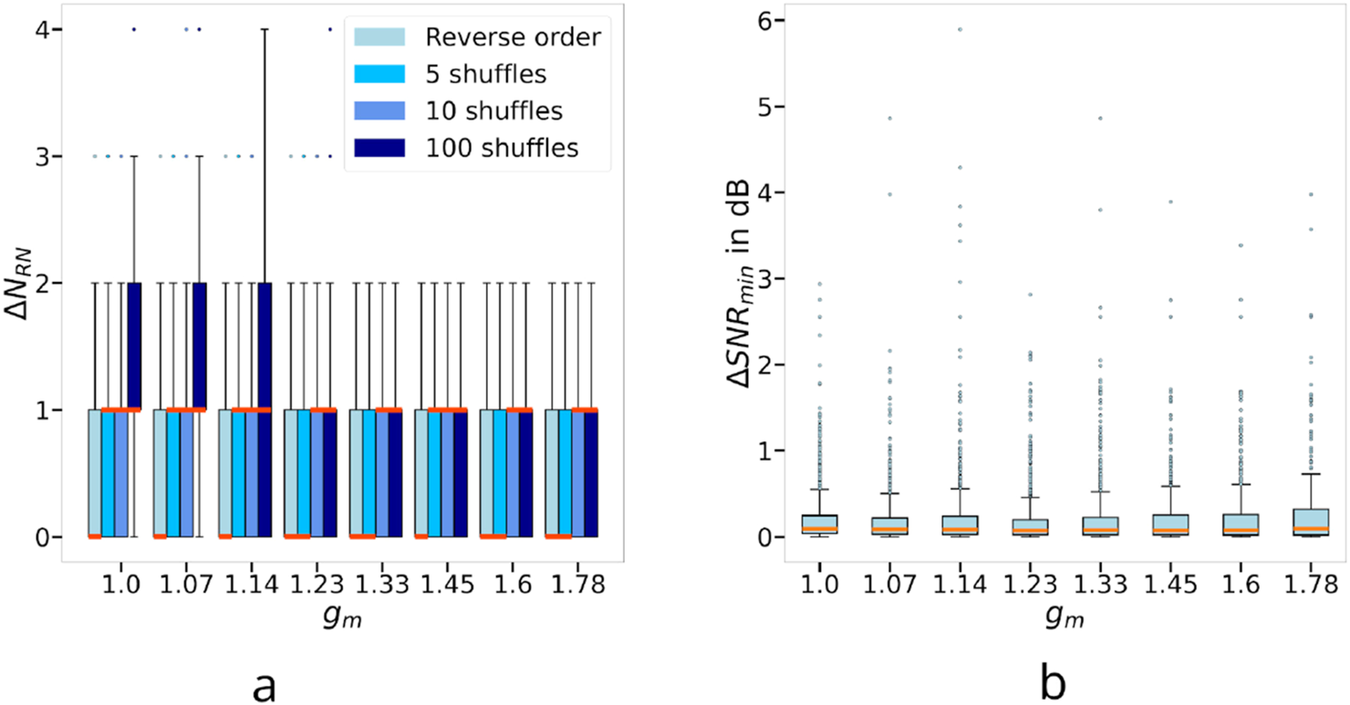
Figure 10. (a) Comparison of the difference in $N_{RN}$ between the result using the initial ordering of segment consideration (0–6) and using the best result among multiple different segment ordering considerations (shuffled segment numbers). (b) Improvement of SNR after realignment using the ORPHe method.

3.2.1 Number of RNs $(N_{RN})$

3.2.1.1 Behavior for increasing $r_{\mathit{min}}$, $r_{\mathit{mid}}$ and $r_{\mathit{max}}$

As it is expected with increasing ranges, all the methods see their $N_{RN}$ decrease as the ranges become larger (see Figure 5a). However, the decrease rate depends on the method. CORP starts with a number of RNs significantly larger than other approaches, with results centered around 20 RNs, but its large decrease rate allows it to close the gap between CORP and MST-1tRN—which decreases the slowest. Both methods have a $N_{RN}$ centered around 10 after an increase in the ranges by a factor of 1.78. Nevertheless, the $N_{RN}$ produced by BHREN is consistently almost half that of CORP and keeps the lowest number of RN among the approaches, starting around 10 and ending around 5.

3.2.1.2 Behavior for $r_{\mathit{mid}}$ and $r_{\mathit{max}}$ growing with respect to $r_{\mathit{min}}$

Figure 5b shows that $N_{RN}$ obtained by CORP stays constant while the two greater ranges, $r_{\mathit{mid}}$ and $r_{\mathit{max}}$, become larger—as it is expected since $r_{\mathit{min}}$ is constant and the CORP method scales with it. On the other hand, the counts of BRHEN and MST-1tRN decrease. They do so at approximately the same rate, thus keeping the same gap between them as $r_{\mathit{mid}}$ and $r_{\mathit{max}}$ increase. BRHEN is the most effective approach, with the bulk initially about 7 RNs and decreasing to about 4. It is followed by MST-1tRN with about 10 to about seven and CORP has the largest number of RNs, staying centered around 13 RNs.

3.2.1.3 Behavior for an increasing number of INs

Finally, Figure 5c depicts the number of RNs required to connect an increasing number of INs. The three methods see their $N_{RN}$ increase with the number of INs. Here again, CORP is the least effective. However, the count of MST-1tRN grows more rapidly, and by the time the number of INs reaches 12, the bulk of the results from MST-1tRN are within the bulk of the results from CORP. BHREN has a lower increase rate than the other approaches and maintains the lowest number of RNs for all the values of the number of INs, staying around half the results from CORP.

3.2.2 Average hop count $(H)$

3.2.2.1 Behavior for increasing $r_{\mathit{min}}$, $r_{\mathit{mid}}$ and $r_{\mathit{max}}$

Figure 6a shows that the average hop counts follows the same pattern as the number of RNs, which is also expected. The notable difference is that MST-1tRN has a decreasing rate similar to that of BRHEN, which keeps MST-1tRN centered around one additional hop from BRHEN.

3.2.2.2 Behavior for $r_{\mathit{mid}}$ and $r_{\mathit{max}}$ growing with respect to $r_{\mathit{min}}$

It can be seen in Figure 6b that $H$ stays constant for CORP, similarly to the $N_{RN}$ results (same reason). However, for BRHEN and MST-1tRN, the results are closer. BRHEN has a lower count for smaller ranges, but MST-1tRN closes the gap for the upper values of the ranges. While $H$ remains centered around 7 for CORP, it is around 5 and around 6 for BRHEN and MST-1tRN, respectively, for the lower range ratio and both are centered under 4 for the largest ratio.

3.2.2.3 Behavior for an increasing the number of INs

In Figure 6c, the average hop count behaves quite differently from the number of RNs. The results are fairly constant for all the approaches. The results of CORP are again almost double that of BRHEN. MST-1tRN generates a slightly higher average hop count than BRHEN.

3.2.3 Number of rounds

The number of rounds performed by the BRHEN algorithm have been counted for different numbers of INs and as a function of the ranges. Figure 7a shows that BRHEN converges in a few rounds for any number of INs. In addition, the number of rounds is inversely proportional to the ranges of the nodes.

3.2.4 Computation time

Similarly to the number of rounds, the computation times of the BRHEN algorithm have been recorded for different numbers of INs and as a function of the range. In Figure 7b, it can be seen that the computation time decreases with increasing ranges for all INs. It is expected because the number of relays—thus the number calculations for the positions—and the number of rounds decrease with increasing ranges. The higher computation time for larger number of INs is also expected, since the number of relays grows with the number of INs.

For a comparison of the computing time of BRHEN with the other methods, see Figure 7c. It shows that the simplest method, MST-1tRN, is the fastest method. Its time stays mostly constant even if the ranges are growing due to the fact that the heavier computational task is finding the edges of the MST—which does not involve the ranges. BRHEN is heavier than MST-1tRN, but nothing compared to the CORP method, which needs to evaluate 9 cells to select the better one.

3.3 Scalability

Let us now analyze the behavior of the different methods for larger-scale networks. To do so, we multiplied by 10 the dimensions of the square area which gives rise to $120\times 120=14400$ cells where we randomly placed 100 to 1,000 INs. The diagonal of 1 cell still corresponds to $r_{\mathit{min}}$. The INs have a randomly assigned range of either $r_{\mathit{min}}$ or $r_{\mathit{mid}}=1.5r_{\mathit{min}}$. The RNs have a range of $r_{\mathit{max}}=2r_{\mathit{min}}$. For the following results, the statistics are from 100 iterations for each number of INs. Figure 8 compares the performance of the three considered methods in terms of the number of relay nodes, $N_{RN}$, and the computation time, $t$, in milliseconds.

The behavior of $N_{RN}$ is presented in Figure 8a. We can see that the CORP method struggles with the up-scaling having to place around 1,500 RNs when there are 100 INs and around 2,700 for 1,000 INs. On the other hand, BRHEN and MST-1tRN require around 400 and 250 INs, respectively. Although MST-1tRN produces better results under 400 INs, with its nonlinear growth, BRHEN has a lower $N_{RN}$ beyond the 400 INs mark. MST-1tRN requires almost 1,500 RNs, while BRHEN only requires around 750 RNs for 1,000 INs. From this change of trend and the nonlinear growth of BRHEN, we can infer that MST-1tRN is more efficient in lower density networks, while BRHEN is for higher density networks. CORP also exhibits this non-linear growth.

The computation time of the three methods behaves similarly as can be observed in Figure 8b. They grow similarly with $N_{IN}$ but their orders of magnitude are different. The lightest method is MST-1tRN which starts at around 200 m for 100 INs and ends at $3\times 10^4$ ms. BRHEN and CORP start at 1,500 m and $1.5\times 10^4$ ms, and end at $4\times 10^4$ and $2\times 10^5$, respectively. The MST-1tRN method remains the lightest even on a larger scale.

3.4 Stability

To manage mobile INs, a RN placement algorithm must produce positions that are stable with respect to the displacements of the INs. In order to assess this stability, for each scenario, the positions of the RNs were compared to the ones of the same scenario after all the INs are moved a certain distance in a randomly chosen direction. The stability is evaluated for different values of the distance, labeled $d_{IN}$.

Two metrics are used for the assessment. The first metric is the average distance between the positions of the initial scenario and the disrupted scenario of each RN—or mean RN displacement. As is easily conceivable, INs moving towards each other or in opposite directions can induce a variation of $N_{RN}$. Thus, the second metric is the probability that $N_{RN}$ changes.

For each value of $d_{IN}$, 1,000 scenarios are randomly generated in the same way as for the previous results. However, since the scenarios do not have to be appropriate for a cell-based method, the map is chosen to be a square with a side length of 1,000 m and the ranges are $r_{\mathit{min}}=100$ meters, $r_{\mathit{mid}}=1.5r_{\mathit{min}}$ and $r_{\mathit{max}}=2r_{\mathit{min}}$. $d_{IN}$ varies from 1 to 10 m. It is 1–10 percent of $r_{\mathit{min}}$. For each value, it produces a variation in distance between the INs of 0–2 times $d_{IN}$ — 0 being the two considered INs displaced towards the same direction, and 2 towards the opposite directions. In this case, it represents 20 percent of $r_{\mathit{min}}$.

3.4.1 Results

It can be seen in Figure 9a that the majority of the data spread more as the $d_{IN}$ grows. Nonetheless, the median remains about equal to $d_{IN}$. The spreading is expected as the growth of $d_{IN}$ increases the probability that the disrupted scenario has a completely different structure—e.g., the first border nodes are different or two nodes are now neighbors. However, this probability exists even for a small $d_{IN}$. This is reflected in the decrease in the number of outliers and their values. On the other hand, the highest values appear to be independent of $d_{IN}$ and may be related to the ratios between the ranges or between the scale of the ranges and the scale of the map.

Figure 9b gives the probability that $N_{RN}$ varies after the perturbation. As expected, this metric increases with $d_{IN}$. This is also due to the growing probability to have a completely different structure. Nonetheless, even for $d_{IN}=10$ meters, it stays below 40 percent.

Now, if we add information on the time within which these displacements occur, we obtain a value for the velocity of the INs. The RNs would have to reach their new position in the same amount of time to prevent the network from partitioning momentarily during these displacements. Therefore, we can study the required RN speed from the results presented in Figure 9a. We can see that the median of $<d_{RN}>$ is around the same value as $d_{IN}$ and the third quartile is slightly above $\approx 2d_{IN}$. Thus, as long as the RNs can move freely around the same speed as the INs, we have a $\approx 50\%$ probability that the RNs can keep up with the changes in positions. Otherwise, a momentary partitioning might occur during that time frame. However, if the RN’s are significantly more mobile than the INs, say twice as mobile, it almost achieves the $75\%$ probability mark.

In order to give a more concrete example, for the chosen range values of $r_{\mathit{min}}=100$ meters $r_{\mathit{mid}}=1.5r_{\mathit{min}}$, $r_{\mathit{max}}=2r_{\mathit{min}}$. Taking the worst scenario presented in Figure 9a where $d_{IN}=10$ meters (or $10\%$ of $r_{\mathit{min}}$). For simplicity, we chose to assume that the displacements occur within 1 s, i.e., the INs are moving at 10 m/s. To obtain around $75\%$ probability that the RNs have time to adjust without possible momentary partitions in the network, the RNs need to reach 20 m/s (or 72 km/h). If we consider UAVs as RNs, this is an achievable speed, even for small ones. Nevertheless, the more reasonable speed of 10 m/s (or 36 km/h) will already reach $50\%$. If we double the ranges, we now have $d_{IN}=0.05r_{\mathit{min}}$. Since $d_{IN}$ is now 5% of $r_{\mathit{min}}$, this scenario corresponds to $d_{IN}=5$ in Figure 9a. 10 m/s and 20 m/s will now allow us to reach between $75\%$ and $95\%$, and almost $75\%$, respectively. Let us point out that the temporary partition that would arise would last around the same time frame as assumed for the displacement.

3.5 Influence of segment consideration order

Upon initiating a scenario, the INs are given a random (or arbitrary) segment number. The BRHEN algorithm uses these numbers to consider the segments in the standard order. However, that order will influence the overall structure of the resulting network, and nothing guarantees that the given order is yielding the best result.

One way to get closer to the best result is to shuffle the segment consideration order a given number of times and take the best of all the outputs. In the following, the output with the least number of RN will be considered the best. We applied this method for 1 shuffle (a simple reversal of the order), 5, 10 and 100 shuffles, using the same parameter $g_m$ and the same number of random scenarios for each parameter value as in Subsection 3.2. This allows us to take the results presented in Figure 5 as a reference for $N_{RN}$ with one run. We obtain a statistical distribution of the number of RNs that we can save by doing each number of shuffles. It is represented by $\mathrm{\Delta }{N}_{RN}=N_{RN}^0-N_{RN}^{\mathit{best}}\ge 0$, with $N_{RN}^0$, the initial result, and $N_{RN}^{\mathit{best}}$, the smallest number obtained among the initial result and the ones given by the different shuffles. The results are presented in Figure 10a.

We can see that from a small number of shuffles (1–5) we already get an appreciable probability that one less RN is deployed. For small values of $g_m$ (small ranges with respect to the area), proceeding to a great number of shuffles can lead to a high probability of reducing $N_{RN}$ even more. Nevertheless, this advantage fades with increasing $g_m$ (with greater ranges). This is expected since $N_{RN}$ decreases with growing $g_m$, thus there are fewer RN that might be superfluous.

These results suggest that doing a few runs of the BRHEN algorithm with shuffled segment orderings has a non-negligible probability of resulting in a better RN layout. Since BRHEN is computationally light, it is a reasonable option. However, for relatively large ranges with respect to the area, a representative sample can consist of only a few shuffled runs.

3.6 Use of the ORPHe method and its effects

With Proposition 2.8, we have shown that using the ORPHe method to place RNs between two nodes allowed the overall SNR between the two to be improved. Here we show that when applied as a realignment method within the BHREN algorithm, we obtain a slight SNR improvement within the segment.

To do so, we are using the same simulation setup as in Subsection 3.2 with $g_m$ as the parameter. Each time a realignment occurs within BRHEN, we calculate the difference between the smallest SNR in the segment being realigned before and after as $\mathrm{\Delta }SN{R}_{\mathit{min}}=SN{R}_{\mathit{min}}^{\mathit{after}}-SN{R}_{\mathit{min}}^{\mathit{before}}$. Since the ranges are assumed to have been computed to achieve a desired SNR (i.e., a desired modulation), $SN{R}_{\mathit{min}}^{\mathit{before}}$ is set. To find $SN{R}_{\mathit{min}}^{\mathit{after}}$, we use Equation 10. Applying the corresponding PLE for a link and the corresponding range, we can extract the $F$ coefficient of that link from the before case, then use $F$ and the new distance between the two nodes to obtain the new SNR of that link. Thus, for each link, we use the formula:

$SN{R}^{\mathit{after}}\left[dB\right]=SN{R}^{\mathit{before}}\left[dB\right]\underset{\mathrm{\Delta }SNR}{\underbrace{+\hspace{0.17em}10\times PLE\times \left(\log r_{\mathit{min}}-\log d\right)}},(21)$

with $PLE$ depending on the type of link and $r_{\mathit{min}}$ the smallest range of the two nodes (which defines the before distance between the two). The improvement in SNR is given by the second term $\mathrm{\Delta }SNR$ and $\mathrm{\Delta }SN{R}_{\mathit{min}}$ will be the smallest value of the second term within the links in the realigned segment. From each BRHEN run, we take the average of those improvements. For the simulations, since $\mathrm{\Delta }SNR$ does not depend on $SN{R}^{\mathit{before}}$ it is unnecessary to specify it. We only have to set the different PLEs and since the RNs are assumed to be UAVs, we have set $PLE=2$ between RNs (i.e., assuming LOS) and $PLE=2.5$ between INs and RNs. Figure 10b shows the statistics of the 1,000 scenarios for each value of $g_m$.

The data suggest that there is always a slight improvement in SNR in the realigned segment after using ORPHe. The median is around 0.1 dB, but in some isolated cases, it can be several dB, with a maximum improvement obtained of 6 dB. The results are mostly the same for all values of $g_m$, this is expected since the relative growth of the ranges might reduce the number of nodes placed, and thus the number of realignments needed. However, the mean improvement of these realignments remains mostly unchanged.

4 Applicability of the BRHEN algorithm

The BRHEN algorithm is a heuristic method that is suitable for 1-tiered heterogeneous networks. The heterogeneity appears in the form of the variety of ranges it takes into account. Behind the difference in ranges is hidden a difference in emitting power, sensibility, propagation path, or a combination of those. In cases where the line between two nodes is not horizontal (such as between air and ground), the range that should be applied is the length of the path as it appears on the horizontal plane.

For example, the placement of ground stations for a permanent or temporary network. The difference in range here will be due to the difference in emitting power and sensibility. Another example is with UAVs as RNs, they enjoy free space LOS propagation for the links between each other, resulting in a greater range between them than between ground nodes with the same radio setup.

This second use-case can be pushed further into the realm of Non-Terrestrial Networks (NTN). However, using greater ranges will result in the need to take into account the Earth’s curvature. Using a conformal projection, which keeps the angles—thus the direction toward the barycenter—true, will allow the method to stick to the Cartesian formulation. Nevertheless, the distances are distorted along the meridians. Due to this, for large areas that span several degrees in latitude, a more complex formulation must be developed for the different steps of the BRHEN algorithm.

5 Conclusion

This paper investigates the methods allowing to manage the RN placement for heterogeneous networks, focusing on their effectiveness regarding the number of Relay Nodes (RNs) placed, the average hop count for the delay, the computation time, and the stability of the placement when the network is nonstatic.

Two algorithms are proposed: ORPHe (Optimized Relay Placement for one Heterogeneous link) for an enhanced RN placement between two disconnected nodes and BRHEN (Barycenter-focused Relay node placement for HEterogeneous wireless Network). They can manage a heterogeneous set of INs and RNs with a different set of communication properties. In addition, it does not require the definition of cells—which limits the precision of the computed positions.

Whether in terms of number of RNs used or in terms of the average hop count for two INs to communicate, the simulations results show the advantage of the BRHEN method over two other approaches for heterogeneous networks. Moreover, BRHEN is shown to be computationally light and to have a relatively good stability. These are important features for mobile networks, since the positions have to be updated frequently—the higher the velocities, the higher the frequency—and the updated RN positions have to be reasonably close to the previous ones. This is an important feature allowing to keep the integrity of the network during readjustments using mobile RNs with reasonable speed.

6 Future works

As a follow-up, strategies to optimally cope with the displacements of the INs need to be explored. First, study predictive IN movements first and, ultimately, deal with unexpected IN motion. Other future work will focus on the implementation of terrain and signal propagation loss in the placement selection process before conducting measurement during field trials for validation.

Data availability statement

The raw data supporting the conclusions of this article will be made available by the authors, without undue reservation.

Author contributions

EG: Conceptualization, Data curation, Formal Analysis, Investigation, Software, Writing – original draft, Writing – review and editing. VL: Writing – review and editing. BL: Writing – review and editing. MB: Writing – review and editing.

Funding

The author(s) declare that financial support was received for the research and/or publication of this article. This research is funded by the Royal Military Academy of Belgium.

Conflict of interest

The authors declare that the research was conducted in the absence of any commercial or financial relationships that could be construed as a potential conflict of interest.

Generative AI statement

The author(s) declare that no Generative AI was used in the creation of this manuscript.

Publisher’s note

All claims expressed in this article are solely those of the authors and do not necessarily represent those of their affiliated organizations, or those of the publisher, the editors and the reviewers. Any product that may be evaluated in this article, or claim that may be made by its manufacturer, is not guaranteed or endorsed by the publisher.

Footnotes

¹The information of the height, $z_A$, is hidden in $r_A$ as the range will be influenced by the propagation channel. If the INs and the RNs have different heights, $r_A$ can be viewed as the projection on the horizontal plane of the 3D $r_A$.

References

Cao, R., Gao, H., Lv, T., Yang, S., and Huang, S. (2016). Phase-rotation-aided relay selection in two-way decode-and-forward relay networks. IEEE Trans. Veh. Technol. 65, 2922–2935. doi:10.1109/TVT.2015.2442622

CrossRef Full Text | Google Scholar

Cheng, X., Du, D.-Z., Wang, L., and Xu, B. (2008). Relay sensor placement in wireless sensor networks. Wirel. Netw. 14, 347–355. doi:10.1007/s11276-006-0724-8

CrossRef Full Text | Google Scholar

Deyab, T. M., Baroudi, U., and Selim, S. Z. (2011). “Optimal placement of heterogeneous wireless sensor and relay nodes,” in 2011 7th international wireless communications and mobile computing conference, 65–70. doi:10.1109/IWCMC.2011.5982508

CrossRef Full Text | Google Scholar

Grönkvist, J., Hansson, A., Hägglund, K., Komulainen, A., and Sköld, M. (2022). Low-altitude uavs for significantly increased data rate in tactical ad hoc networks. Procedia Comput. Sci. 205, 107–116. doi:10.1016/j.procs.2022.09.012

CrossRef Full Text | Google Scholar

Han, X., Cao, X., Lloyd, E. L., and Shen, C.-C. (2010). Fault-tolerant relay node placement in heterogeneous wireless sensor networks. IEEE Trans. Mob. Comput. 9, 643–656. doi:10.1109/TMC.2009.161

CrossRef Full Text | Google Scholar

Ladosz, P., Oh, H., and Chen, W.-H. (2018). Trajectory planning for communication relay unmanned aerial vehicles in urban dynamic environments. J. Intelligent Robotic Syst. 89, 7–25. doi:10.1007/s10846-017-0484-y

CrossRef Full Text | Google Scholar

Lee, S., and Younis, M. (2010a). Optimized relay placement to federate segments in wireless sensor networks. IEEE J. Sel. Areas Commun. 28, 742–752. doi:10.1109/JSAC.2010.100611

CrossRef Full Text | Google Scholar

Lee, S., and Younis, M. (2010b). “Qos-aware relay node placement for connecting disjoint segments in wireless sensor networks,” in 2010 6th IEEE International Conference on Distributed Computing in Sensor Systems Workshops (DCOSSW), Santa Barbara, CA, USA, 21-23 June 2010, 1–6. doi:10.1109/DCOSSW.2010.5593290

CrossRef Full Text | Google Scholar

Lee, S., and Younis, M. (2010c). Recovery from multiple simultaneous failures in wireless sensor networks using minimum steiner tree. J. Parallel Distributed Comput. 70, 525–536. doi:10.1016/j.jpdc.2009.12.004

CrossRef Full Text | Google Scholar

Lin, G., and Xue, G. (1999). Steiner tree problem with minimum number of Steiner points and bounded edge-length. Inf. Process. Lett. 69, 53–57. doi:10.1016/s0020-0190(98)00201-4

CrossRef Full Text | Google Scholar

Liu, G., Lu, K., and Li, J. (2019). “Approximation algorithm for relay node placement in singled-tiered wireless sensor networks,” in 2019 IEEE 4th International Conference on Advanced Robotics and Mechatronics (ICARM), Toyonaka, Japan, 03-05 July 2019, 162–167. doi:10.1109/ICARM.2019.8834312

CrossRef Full Text | Google Scholar

Lloyd, E. L., and Xue, G. (2007). Relay node placement in wireless sensor networks. IEEE Trans. Comput. 56, 134–138. doi:10.1109/TC.2007.250629

CrossRef Full Text | Google Scholar

Parihar, A. S., Baghel, A., Swami, P., and Bhatia, V. (2024a). “On performance of swipt empowered noma-hetnet with non-linear energy harvesting,” in 2024 national conference on communications (NCC), 1–6. doi:10.1109/NCC60321.2024.10485896

CrossRef Full Text | Google Scholar

Parihar, A. S., Singh, K., Bhatia, V., Li, C.-P., and Duong, T. Q. (2024b). Performance analysis of noma-enabled active ris-aided mimo heterogeneous iot networks with integrated sensing and communication. IEEE Internet Things J. 11, 28137–28152. doi:10.1109/JIOT.2024.3416951

CrossRef Full Text | Google Scholar

Robins, G., and Zelikovsky, A. (2005). Tighter bounds for graph steiner tree approximation. SIAM J. Discrete Math. 19, 122–134. doi:10.1137/S0895480101393155

CrossRef Full Text | Google Scholar

Swami, P., and Bhatia, V. (2021). “Impact of distance on outage probability in irs-noma for beyond 5g networks,” in 2021 IEEE 18th Annual Consumer Communications Networking Conference (CCNC), Las Vegas, NV, USA, 09-12 January 2021, 1–2. doi:10.1109/CCNC49032.2021.9369548

CrossRef Full Text | Google Scholar

Swami, P., Mishra, M. K., Bhatia, V., Ratnarajah, T., and Trivedi, A. (2022). Performance analysis of sub-6 ghz/mmwave noma hybrid-hetnets using partial csi. IEEE Trans. Veh. Technol. 71, 12958–12971. doi:10.1109/TVT.2022.3198144

CrossRef Full Text | Google Scholar

ur Rahman, S., Kim, G.-H., Cho, Y.-Z., and Khan, A. (2018). Positioning of uavs for throughput maximization in software-defined disaster area uav communication networks. J. Commun. Netw. 20, 452–463. doi:10.1109/JCN.2018.000070

CrossRef Full Text | Google Scholar

Wang, Z., Duan, L., and Zhang, R. (2019). Adaptive deployment for uav-aided communication networks. IEEE Trans. Wirel. Commun. 18, 4531–4543. doi:10.1109/TWC.2019.2926279

CrossRef Full Text | Google Scholar

Wu, Y., Zhang, B., Yang, S., Yi, X., and Yang, X. (2017). “Energy-efficient joint communication-motion planning for relay-assisted wireless robot surveillance,” in IEEE INFOCOM 2017 - IEEE Conference on Computer Communications, Atlanta, GA, USA, 01-04 May 2017, 1–9. doi:10.1109/INFOCOM.2017.8057072

CrossRef Full Text | Google Scholar

Xie, J., Zhang, B., and Zhang, C. (2020). A novel relay node placement and energy efficient routing method for heterogeneous wireless sensor networks. IEEE Access 8, 202439–202444. doi:10.1109/ACCESS.2020.2984495

CrossRef Full Text | Google Scholar

Yang, S., Xu, X., Alanis, D., Xin Ng, S., and Hanzo, L. (2016). Is the low-complexity mobile-relay-aided ffr-das capable of outperforming the high-complexity comp? IEEE Trans. Veh. Technol. 65, 2154–2169. doi:10.1109/TVT.2015.2416333

CrossRef Full Text | Google Scholar

Yanmaz, E. (2021). Dynamic relay selection and positioning for cooperative uav networks. IEEE Netw. Lett. 3, 114–118. doi:10.1109/LNET.2021.3080403

CrossRef Full Text | Google Scholar