Abstract
Introduction:
With the rapid evolution of vehicular networks, delay-sensitive applications such as autonomous driving and real-time navigation have gained significant attention. However, vehicles with limited computational resources often fail to meet low-latency demands, creating a critical bottleneck in system performance.
Methods:
To address this challenge, we propose the use of Mobile Edge Computing (MEC) for offloading time-sensitive tasks to roadside servers, reducing response times through localized processing and network intelligence. A mathematical model based on Markov Chains was developed to capture traffic dynamics and response behaviors in vehicular environments. This model enables analytical performance evaluation without relying on time-consuming simulations.
Results:
Experimental evaluation shows that the analytical model provides predictions consistent with simulation outcomes. Specifically, for vehicle counts ranging from 20 to 120, the model estimated average response times between 0.023–0.505 s, closely matching the simulation baseline of 0.019–0.482 s. The relative error was between 3.4% and 24.0%, with a mean of 11.7%.
Discussion:
The results validate the practicality and effectiveness of the proposed approach in meeting delay-sensitive requirements. Beyond vehicular networks, the modeling framework can also be extended to support smart campus initiatives, including mobility solutions, IoT management, and intelligent infrastructure systems, highlighting its broader applicability in advancing smart technologies.
1 Introduction
Computer networks have become crucial for transmitting information in today’s world. One project that stands out for its usefulness and efficiency in improving the quality of human life is the discussion of vehicular networks (Gerla and Kleinrock, 2011; Kanthasamy and Wyglinski, 2025; Son et al., 2025). The safety of vehicles during movement has always been a driving force behind new traffic ideas and plans. In recent years, there has been a pursuit of new ideas, including the development of a Vehicular Ad hoc Network called VANET (Sahu et al., 2024). VANET is a communication network that connects smart vehicles, as well as fixed and mobile resources along the road, effectively organizing them (Rajkumar and Kumar, 2024). A vehicular network comprises both vehicles and network infrastructure. Intelligence is enabled in automotive networks through the utilization of Mobile Edge Computing (MEC) technology (Mao et al., 2017a). By leveraging MEC technology, one can experience advantages like minimizing latency and accessing limitless cloud resources (Wu et al., 2019).
The rapid growth of vehicular networks has given rise to software that is sensitive to delays, such as automatic driving and automatic navigation. These software applications require significant processing power to handle the large amount of data they deal with.
Also, the implementation of computer networks, particularly vehicular networks, is always a significant concern and challenge in various areas of computer science. When it comes to implementation, there are consistently two challenges (Quadar et al., 2024; Wu et al., 2024; Pang and Wang, 2024; Hemmati et al., 2024). The first challenge revolves around the costs associated with implementation, while the second challenge focuses on the delay in package delivery. Generally, these two topics are interconnected, as the aim is to minimize package delivery delays while keeping costs as low as possible. One common approach to achieving an optimal network is through implementation, which can be costly in terms of both time and money. However, there is an alternative method known as simulation, which is more financially feasible but requires a considerable amount of time. Another method that aids in verifying desired factors such as cost reduction, speed of achieving results, and an accurate assessment of network efficiency is the evaluation or mathematical modeling of the network. By employing this method, it becomes possible to gain a reasonable understanding of the efficiency of the existing conditions of the network, even before implementation or simulation takes place. However, vehicles with limited resources often struggle to provide the desired level of service quality, as they are sometimes hindered by processing delays.
In this study, we aim to address this issue by offloading some of the delay-sensitive tasks to roadside and cloud servers. By using Markov chains in various modes, we assess the available delays and average response time in a vehicular network (Ram et al., 2019). In summary, the proposed methodology entails the examination of a vehicular network consisting of three groups of nodes: 1- Mobile nodes (vehicles) 2- Stationary Roadside Units (RSUs) 3- Cloud. Initially, a Markov chain with a finite queue is considered for each group of nodes. Subsequently, various processing modes, such as local processing or sending to another processing unit, are evaluated for each group. Ultimately, a final relationship is established for each group, indicating the rate of return from the states of the nodes. The next step involves utilizing this relationship and inputting it into the Symbolic Hierarchical Automated Reliability and Performance Evaluator (SHARPE) software to obtain the probability of being present in each state. With this probability, the average number of jobs in the queue is calculated, and subsequently, the average response time of the network is determined using Little’s law. The proposed method evaluates the efficiency of the vehicular network through mathematical modeling utilizing Little’s law and Markov chains. Efficiency, in this context, refers to the ability to predict the suitability of the network’s response time without the need for implementation or simulation, considering the number of vehicles, RSU-connected servers, and the utilization of powerful cloud resources. Little’s law is an independent law of modeling, while Markov chains possess memoryless properties, meaning that the current state does not correlate with previous steps. Several Markov chain models exist, with this research employing the continuous-time Markov chain (CTMC) model. This method treats time as an instantaneous moment, eliminating the presence of loops. It should be noted that due to the mobility of vehicular networks, there are many possibilities such as variable network density, weather conditions and other driving-related factors in the real world. In this study, we have considered the vehicular network in a steady state, meaning that we have observed and monitored the network for a long time and have obtained an average of the network traffic data. This indicates that the data used in our calculations is a close approximation and not necessarily all the conditions governing vehicular networks have been considered. The modeled environment represents a MEC-enabled vehicular (V2X) network over a 5G/6G-ready architecture in which RSUs act as edge servers and resources are provisioned via logical network slicing.
The remaining part of the paper is organized as follows: In Section 2, there is a comprehensive analysis of the latest literature. Section 3 offers an in-depth explanation of the proposed method. The evaluation of the performance and results of the proposed method is deliberated in Section 4. Lastly, Section 5 wraps up the study with a brief overview and future work.
2 Related works
In the last few years, there has been a lot of interest in MEC, and many researchers have conducted extensive research in this area (Wang et al., 2017; Ansari and Sun, 2018). Specifically, some of them concentrated on the issue of deciding when to offload tasks (Guo and Liu, 2018; Guo et al., 2018), while others tackled the broader problem of allocating and managing computing resources for radio (Mao et al., 2017b; Rodrigues et al., 2018). Recent works in 2024–2025 have also investigated MEC-enabled vehicular networks with deep reinforcement learning for offloading/scheduling and hybrid stochastic queueing models; the revised text now contextualizes our model against these advances (Rajkumar and Kumar, 2024; Quadar et al., 2024; Pang and Wang, 2024).
Chao et al. studied the task offloading problem in highly dense networks and proposed a heuristic greedy offloading scheme to minimize the energy consumption of mobile devices under the constraints of acceptable task processing time (Chao and Pinedo, 1999). Lai et al. (Lai et al., 2010) investigated the multi-user computational offloading problem in a multi-channel wireless interference environment and proposed a computational offloading algorithm based on distributed game theory to minimize the computational overhead of mobile users. To reduce the energy consumption of mobile devices and MEC servers, Mao et al. proposed a scheme that jointly optimizes radio resource allocation and computing resource management (Mao et al., 2017b). Specifically, they used a closed-form approach to derive the optimal CPU cycle frequency of mobile devices and MEC servers and obtained the optimal transmission power and bandwidth allocation using the Gauss-Seidel method.
In recent years, a significant amount of research has been dedicated to integrating vehicular networks and MEC to address the conflict between delay-sensitive applications and resource-constrained vehicles (Wang et al., 2017; Ansari and Sun, 2018; Mao et al., 2017b). Dai et al. conducted a study to maximize the benefits of MEC service providers by investigating the task offloading problem in Vehicular Edge Computing Networks (VECN) with multiple users and multiple servers (Dai et al., 2018). They approached this problem by formulating it as a combinatorial nonlinear programming problem. To solve it, they divided it into two sub-problems and proposed an optimization algorithm that jointly optimized the MEC server selection procedure and the task offloading decision procedure. Another study by Liu et al. focused on the cost minimization problem in VECNs (Liu et al., 2018). They proposed a distributed algorithm based on game theory to reduce the total computational overhead of vehicle computing tasks.
Many research works have been conducted on the integration of SDN and vehicular networks, which is the main topic of this research (Rodrigues et al., 2018; Yang et al., 2008; Zhang et al., 2019). Huang et al. utilized SDN to centrally manage vehicle communication traffic and put forward a network state routing algorithm based on a lifetime to transmit data through vehicle-to-vehicle (V2V) communication paths in ad networks (Huang et al., 2018). There are vehicular hoc (VANETs), and offload. Liu et al. proposed a scheme that combines various types of access technologies to reduce the processing delay of delay-sensitive applications (Liu et al., 1995). Extensive numerical results demonstrated that their suggested architecture greatly enhances the quality of user experience.
3 Proposed methods
Mathematical modeling of the network allows us to evaluate the performance of the network acceptably without implementing the network or even simulating it. In the process of mathematical modeling and the formulas that are obtained according to it, it is very important to match its results with what happens in the real world. One of the advantages of network mathematical analysis is its low costs in terms of time and money.
In our proposed method, we computed the average response time in vehicular networks using Markov chains and rules governing computer networks. We have considered the Poisson distribution and the queuing model as M/M/1, and time has also been considered as continuous. This type of modeling indicates that no two packets enter the switch at the same time and we have considered the time as an instant. The proposed architecture of task transmission in a vehicular edge-computing network is shown in Figure 1.
FIGURE 1

The proposed architecture of task transmission in a vehicular edge computing network.
Our proposed method is to calculate the average queue and average response time in vehicular networks using the Markov method. In this method, we calculated the mentioned parameters without implementation or even simulation and only using mathematical modeling, and we show that the results are close to reality to an acceptable extent.
Random processes are one of the modeling theories based on statistics and probability and are used for data analysis. In most cases, random processes are listed or indexed by time. Markov Chain or Markov Process is a model for representing a sequence of random variables in which the probability of each event depends only on the previous event. In this way, the probability of the occurrence of events in such a model is only dependent on the previous time and the rest of the events do not interfere with the probability. Such a situation is sometimes called memory less for a random process. This model is called the Markov model or Markov chain in honor of the Russian mathematician Andrey Markov who innovated in this field in the early years of the 20th century. If a random experiment is such that the occurrence of an event is related to a unit of space or time, a Poisson experiment is formed. This name was chosen due to the research of the French scientist Simone Poisson in this field.
There are two types of Markov chains: 1- Discrete-time (DTMC) and 2- Continuous-time (CTMC). In Markov chains in our proposed method, the states represent the number of requests in the queue. As mentioned, one of the characteristics of Markov chains is the property of being memoryless, which means that being in any state has nothing to do with what state we were in before. In continuous-time Markov chains, we do not have loop time because it is instantaneous. But in discrete-time Markov chains, because we consider time as an interval, each state can have a loop. Using Markov chains and finite queues and considering time instantaneously makes our calculations more accurate and reliable.
In queuing theory, the queuing model is used to estimate the real queuing state of the system; therefore, the queue behavior can have a mathematical analysis. Queuing models can use Kendall symbols. These symbols are A/B/S, respectively:
A: represents the arrival interval distribution
B: represents the service time distribution
S: indicates the number of servers
Perhaps the most common queuing situation we encounter in real life is single-server queues. In many situations, we encounter a single server queue. The M/M/1 model implies that we have a queue with one server, unlimited capacity, and unlimited population calls. M/M/1 indicates that the input and output are both based on Poisson distribution and the service time is exponentially distributed. The queue we want to model the network, both for mobile nodes (vehicles) and roadside fixed units (RSU), is the M/M/1/K queue (K is the maximum number of requests in the system). In the M/M/1 queue, the input of the network is with Poisson distribution rate (λ) and the output is with Poisson distribution rate. The processing time is exponentially distributed and all requests are served at the rate μ (μ is the request processing rate per unit time). An example of a vehicular network is shown in Figure 2.
FIGURE 2
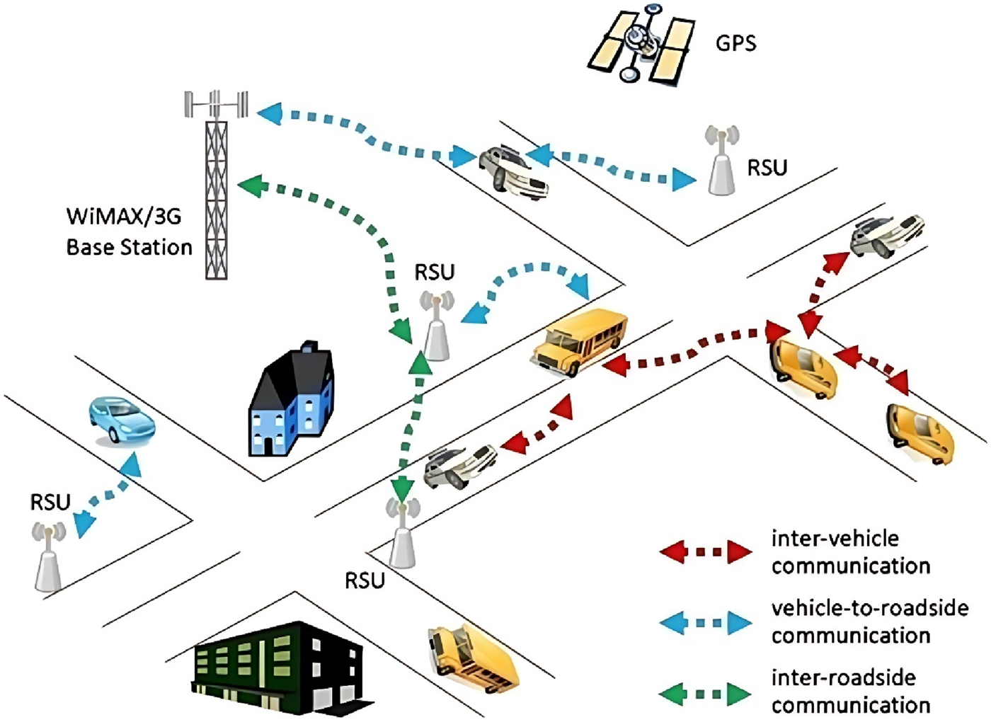
An example of a vehicular network (Eiza et al., 2013).
In our proposed model, the nodes in the network are divided into three parts:
1. Mobile nodes (vehicles) 2- Roadside fixed units (RSUs) 3- Cloud. For each of these sections, we consider a Markov chain with a finite queue.
By formulating these chains for each section, we reach a final relationship and with the help of this relationship, we calculate the rate of return from different states for each of the nodes. Finally, with the help of SHARPE software, which is a popular software for calculating the efficiency of computer networks, we simulate the results and evaluate their accuracy. Also, with the help of SHARPE software, we determine the probability of being in each state, and with this probability, we calculate the average queue. In Figure 3, we show a view of the Sharpe software workspace where we performed calculations related to the probability of being in each state. You can also see an abstract drawing of Markov chains in this software. In the following, for the purpose of better clarity, inspired by the Markov chains drawn in Sharpe software, we have drawn the chains manually, which can be seen in Figures 4–7.
FIGURE 3

The view of the sharpe software workspace.
Finally, using Little’s law, we get the average response time. Little’s law is a theorem written by John Little and is used in queuing theory and states that:
The average number of customers in the long term in a stable system (L) is equal to the average effective entry rate in the long term (λ) multiplied by the average time the customer is in system (W) or algebraic language, i.e., L = λW. The remarkable point is that this relationship is not affected by the distribution of the input process or the distribution of the service process or service order and practically no other factor.
We used Markov chains to model the events in the target network. It is necessary to state that we consider the network to be stable and indifferent to momentary events. The meaning of steady state is that we have monitored the system for a long time, and during this long time, ρ means that the ratio of input load to service time ρ = λ/μ is smaller than one (ρ < 1). In Table 1, you can see the variables used in this study.
TABLE 1
| Symbol | Description |
|---|---|
| WN (job/s) | The average response time of mobile nodes (vehicles) |
| WRSU (job/s) | Average response time of fixed roadside units |
| p | The possibility of sending a request to RSU |
| 1-p | The possibility of local processing on mobile nodes |
| q | The possibility of sending to Cloud |
| 1-q | Possibility of local processing in RSU |
| λ N (job/s) | The rate of arrival of packets to a mobile node based on Poisson distribution |
| λ R (job/s) | Packet arrival rate to RSU based on Poisson distribution |
| λ C (job/s) | The rate of arrival of packets to the cloud-based on Poisson distribution |
| k | Density or the number of vehicles or mobile nodes |
| m | Number of RSUs |
| μN | The service rate of packages in Nod siyar |
| μR | Service rate of packages in RSU |
| μC | The service rate of packages in the Cloud |
| The average queue of mobile nodes | |
| The average queue of mobile nodes | |
| Average cloud queue | |
| The probability of request i being in the mobile node queue | |
| The probability of the request i being in the RSU queue | |
| The probability that request i is in the Cloud queue | |
| Lambda is a real mobile nodes | |
| Real lambda RSU | |
| Real lambda Cloud |
Variables used in the study.
The variables used in our experiment are shown in Table 1.
In the following, we presented the chains related to each of the sections and provided relevant explanations. It should be noted that we consider the queue capacity to be 10 for each section. In each of the sections, we will have two types of processing possibilities: 1- The possibility of local processing and 2- The possibility of sending to the next processor node.
3.1 Mobile queue model
Using Markov chains, we modeled the events of our desired network. In our proposed model, the request-receiving node checks the possibility of local processing by checking its resources. If it has enough resources for processing, it will process the request and return the result to the requesting node, otherwise, it will send it to the upstream node to decide for processing.
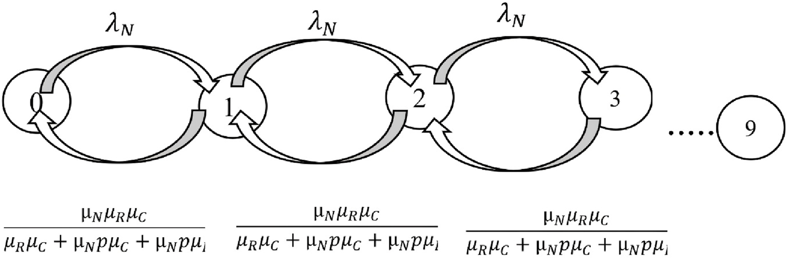
In Figure 4, we can see the chain related to the ninety-sir. As can be seen in this image, we indicate the request arrival rate with λN (job/s) and the response rate with WN(job/s). Here, we consider the probability of local processing as 1-P and the probability of sending to the upstream node, i.e., RSU, as p. The maximum number of requests in the queue can be 10. Requests are sent to the processing nodes with a Poisson distribution and at a rate of λN. Because our Markov chain model is CTMC, therefore we do not have loops. Finally, taking into account these possibilities and the required calculations, we reach a final relationship, with the help of this relationship, we calculate the return rate from the State, or in other words, the average response time (WN) for mobile nodes. You can see the details of the calculations are presented in Equation 1.
FIGURE 4
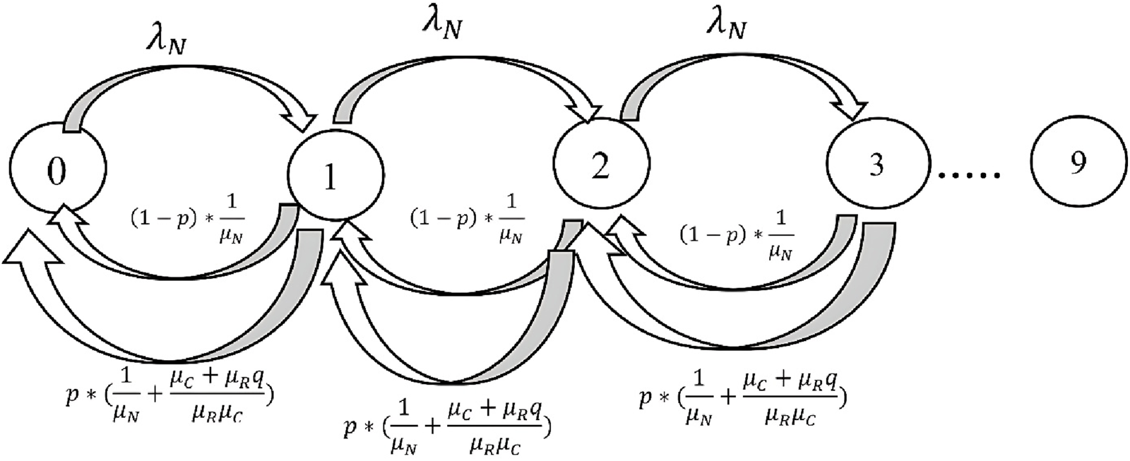
Queuing modeling for mobile nodes (vehicles) with Markov chains.
3.2 RSU queuing model
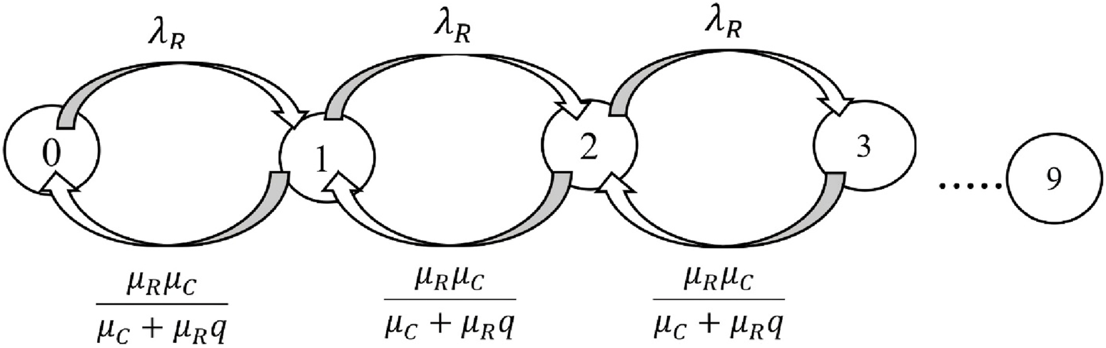
In Figure 5, the Markov chain related to RSU nodes or roadside fixed units is shown. As seen in this image, we denoted the request arrival rate by λR (job/s) and the response rate by. Here, we considered the probability of local processing as 1-q and the probability of sending to the Cloud as q. Finally, considering these possibilities and required calculations, we arrive at a final relationship, with the help of this relationship, we calculate the return rate from the state (State) or in other words, the average response time () for RSU Nodes.
FIGURE 5
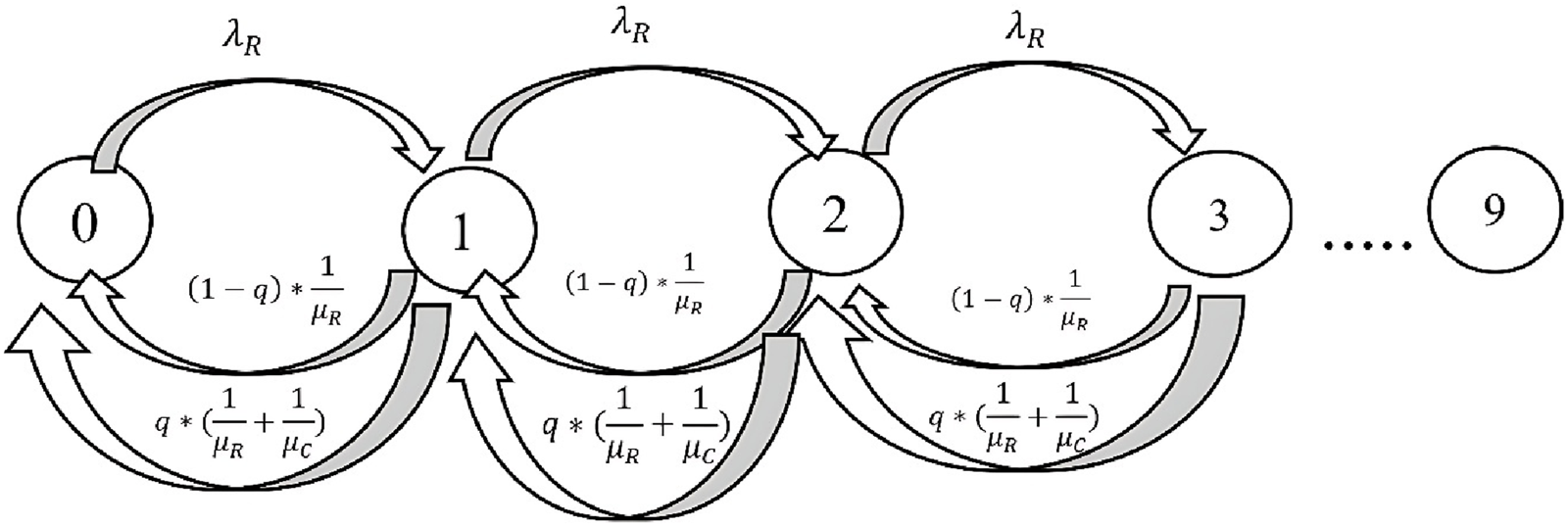
Queuing modeling for stationary RSU roadside units with Markov chains.
One thing that should be noted is the calculation of the request entry rate to RSU, i.e., λR (job/s), which is obtained from Equation 2. Due to the mobile nature of nodes (vehicles), the density or the number of vehicles changes at any moment, hence we defined a variable named k as a representative of this parameter and consider it as input to RSU in Lambda’s calculations. The relevant calculations are presented in Equations 2, 3.
3.3 Cloud queuing model
In Figure 6, we see the chain related to Cloud. As can be seen in this image, we show the request arrival rate with λC and the response rate with μC. Since we consider the system to be linear in the cloud, as a result, the average response time will be equal to the service rate, i.e., μ3. Regarding the exact rate of requests entering the Cloud, or λC, we define another variable called m to represent the number of RSUs located in the study area, and as a result, we calculate the input rate to the Cloud according to the following Equation 4.
FIGURE 6
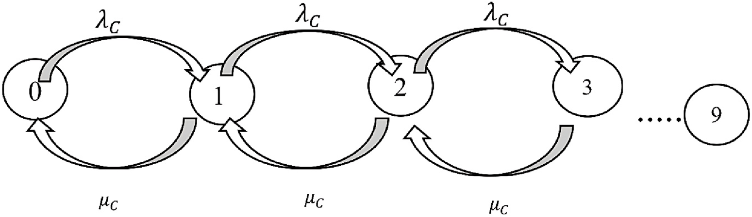
Proposed Markov chain for cloud.
3.4 Queue calculation in linear models
The proposed Markov chain models for the mobile node queue and the RSU queue are not linear by default, and to work with our desired software (SHARPE), all the proposed models, such as the Cloud model, must be presented linearly. Therefore, the models should be slightly edited, with the results presented for the mobile node and the RSU, respectively, as shown in Figures 7, 8.
FIGURE 7
Linearized Markov chain model for mobile node (vehicle).
FIGURE 8
Linearized Markov chain model for RSU.
In our proposed Markov chains, the queue length of ninety mobiles is calculated based on Equation 5:
3.5 Calculate the response time
One of the problems we face in the proposed model is the limited queue problem. A bounded queue means that all incoming requests cannot be queued. This means that our initial entry rate is not the actual entry rate. For example, if the network is facing 10 requests in a steady state, our lambda is the initial arrival rate until the queue is full. As soon as the queue is full, the packets are not placed in the queue. The actual entry rate is calculated from the initial entry rate in the form of Equations 6–8.
Unless otherwise stated, response times are measured in seconds (s) and rates in s-1. We use Little’s law to calculate the response time. Regardless of the type of structure and modeling, Little’s law examines the response time of the network at each stage. The general equation of Little’s law is as Equation 9. We adopted standard M/M/1/K notation with ρ = λ/μ < 1, blocking probability P_block = ((1−ρ)ρK)/(1−ρ{K+1}), effective arrival λ_eff = λ(1−P_block), mean number in system L, and average response time W = L/λ_eff.
By substituting Equations 5, 6 in Equation 9, we reach Equation 10.
Finally, the output of the above equation is the average response time of the mobile node, which can be calculated separately for each of the other nodes in the network.
4 Results and discussion
In this section, we will present the results of the mathematical modeling of the vehicular network using the proposed method. As mentioned in the previous chapter, the software used in the Markov mathematical modeling section is SHARPE software. This software normally considers the M/M/1/K queuing model. One of the features of SHARPE software is that we can define the network model in layers and connect these layers. The primary output of this software is the probability of being present in each state. We have performed calculations related to average queue length and average response time in vehicles as mobile nodes and fixed roadside units (RSUs) as well as the cloud. Finally, using Python software, we will put the data analysis output on the graph. The results show well the behavior of the network in the face of changes in the number of network nodes, including mobile nodes or the number of RSUs, or the increase in requests to these nodes.
4.1 Evaluation of the results
In the review and evaluation of the results and calculations, the following assumptions are considered.
The ratio is always considered less than one (Ride, 1976).
The model of vehicle queue, RSUs, and Cloud is limited and in the form of M/M/1/K.
CTMC Markov chain modeling is considered.
ρ must be less than one, which means that the input of requests must be less than the output, and this is the condition of network stability.
In the M/M/1/K queue model, the input and output of packets are with Poisson distribution rate, and the responding server is a number and the length of our queue is limited to K. In other words, in this model, we have considered the size of the job queue to be equal.
The use of Markov chains is very useful for modeling queues in networks. One of the characteristics of Markov chains is their memoryless property.
CTMC Markov chain modeling has its characteristics. In this modeling, using the balanced relationships between inputs and outputs, they calculate the probability of being in each state. Since in CTMC time is calculated in moments, two requests cannot enter nodes at the same time. As a result, we do not have a loop. Now, according to these characteristics, we check the queue status and the average response time in vehicular networks.
4.1.1 Investigating the changes in the mobile node queue due to the increase in lambda
The rate of arrival of packages to the vehicle is considered by Poisson distribution and by Lambda rate. The dataset included in this article was generated and used during the research process and based on logical reasons and other assumptions and possibilities in a vehicular network. To generate this dataset, we considered the nature of vehicular networks such as vehicle speed, density, distances, direction of movement, etc. and independently generated the data required for mathematical calculations of the vehicular network, including arrival rate, service rate, node processing capacity, and probabilities of occurrence of each state. Then, by changing the desired data, we examined and monitored the behavior of the network. At first, the vehicle processing rate is considered 35, and the arrival rate of packages changes between 10 and 34. The parameters related to the investigation of changes in the vehicle queue based on the increase of Lambda are presented in Table 2.
TABLE 2
| Variable | P | q | K | m | |||
|---|---|---|---|---|---|---|---|
| Value | 35 | 0.06 | 55 | 75 | 0.06 | 5 | 5 |
Data used in analyzing changes in vehicle queues based on lambda changes.
First, we needed to check that our condition about ρ < 1 is not violated. Checking the condition of ρ < 1 based on the changes in the vehicle queue with the increase of Lambda is shown in Table 3.
TABLE 3
Analysis of the condition ρ < 1 based on the changes in the vehicle queue with lambda changes.
We checked the worst case:
The changes in the mobile node (vehicle) queue diagram are shown in Figure 9.
FIGURE 9
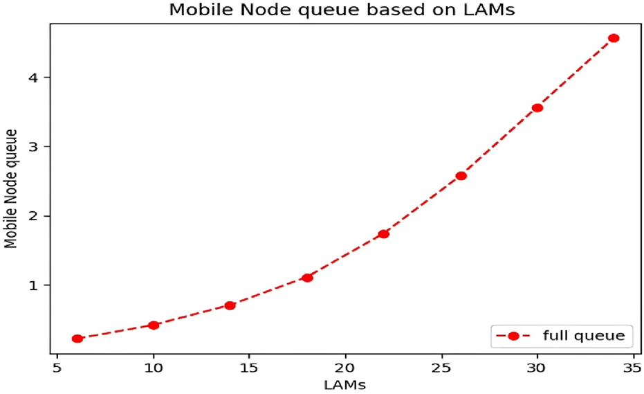
The changes in the vehicle queue are due to the increase in Lambda.
Here, we have considered a limited vehicle queue of 9 requests. At first, the vehicle queue increases with a gentle slope, but with the increase of Lambda in the range of 18, this slope becomes steeper and the efficiency decreases. The reason for this is that with the increase in incoming traffic, there is a possibility that some requests will go to RSU, and this will prolong the response time and increase the queue length in mobile nodes.
Table 4 shows the effect of the vehicle entrance on the vehicle queue, RSU and Cloud.
TABLE 4
| 6 | 10 | 14 | 18 | 22 | 26 | 30 | 34 | |
|---|---|---|---|---|---|---|---|---|
| 0.224 | 0.422 | 0.710 | 1.113 | 1.742 | 2.575 | 3.566 | 4.564 | |
| 0.035 | 0.060 | 0.086 | 0.114 | 0.136 | 0.173 | 0.205 | 0.240 | |
| 0.0072 | 0.012 | 0.017 | 0.022 | 0.027 | 0.032 | 0.037 | 0.042 |
Results from changing vehicle arrival rates on RSU and cloud vehicle queues.
By checking the entries in the above table, it can be seen that with the addition of the input Lambda, while the rest of the variables remain constant, the queue of the mobile node (vehicle) changes a lot, but there is no significant change in the queue of RSU and Cloud. The point that we need to pay attention to is that the above numbers were obtained in stable mode.
4.1.2 Investigating the mobile node queue with simultaneous lambda and P changes (possibility of sending to RSU)
Here, we intend to Investigate the vehicle queue while the variable P, which means the probability of sending to the RSU, changes at the same time as Lambda changes. Increasing this probability means that a large part of the packages cannot be processed by the vehicle due to reasons such as package size or processing resource limitations and are transferred to the RSU. We considered other variables as the values in Table 5 and investigated the worst case.
TABLE 5
Analysis of the condition ρ < 1 for vehicle queues considering variations in lambda and probability P.
Based on Table 5, First, we have to check that our condition about ρ < 1 is not violated. The investigation of establishing the condition ρ < 1 about the vehicle queue with changes of Lambda and P is presented in Table 5.
As can be seen in Figure 10, when the network input or Lambda and the probability of sending to RSU increase simultaneously, as expected, in low Lambda, there is no significant effect on the number of jobs in the mobile node queue, but in high Lambda, the number The packets in the queue will increase with a relatively higher slope, and if this process continues, knowing that our queue is limited to K, the possibility of discarding the requests will increase, and practically, our network will not be very efficient.
FIGURE 10
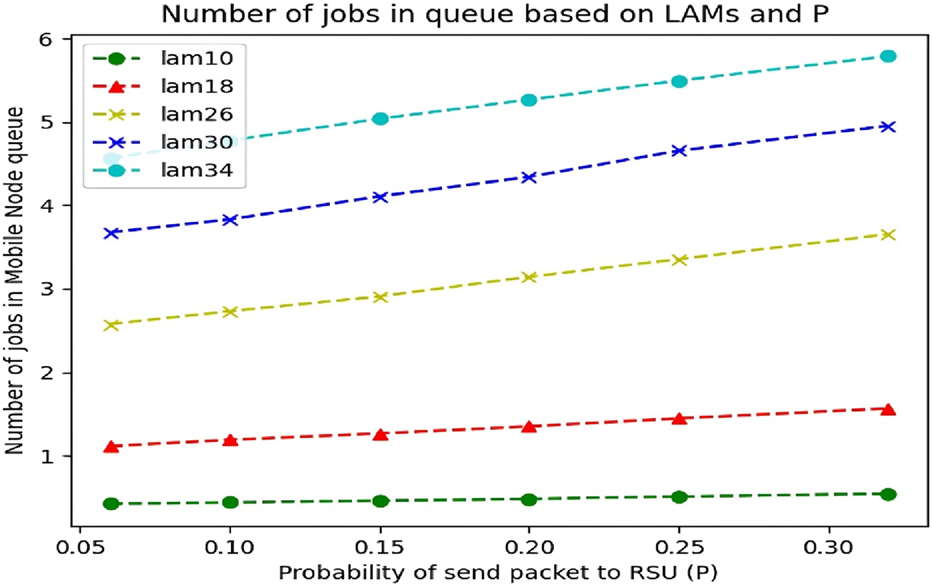
Vehicle queue changes due to the simultaneous changes of lambda and P.
When we calculate the graph of the average response time of the vehicle with these variables, we reach similar results. Figure 11 expresses the matter well.
FIGURE 11

The average response time of mobile nodes according to the simultaneous changes of lambda and P.
In Figure 11, we see the linear growth of the response time. The interesting thing to note in this diagram is the convergence of the results with diagram 10 so that the increase of the p variable in the low Lambdas does not cause a significant change in the average response time of the vehicle, but in the high Lambdas, the intensity of the changes is greater and, as a result, the average response time has a relatively greater slope. Is increasing The next point is that the response times on larger Lambdas are not significantly different, meaning that we are increasing the input Lambda as well as increasing the P variable, but our average response time does not change significantly. The reason for this can be seen in Figure 12.
FIGURE 12
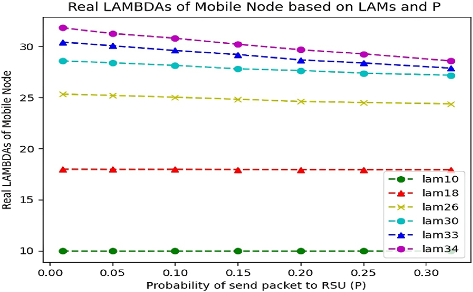
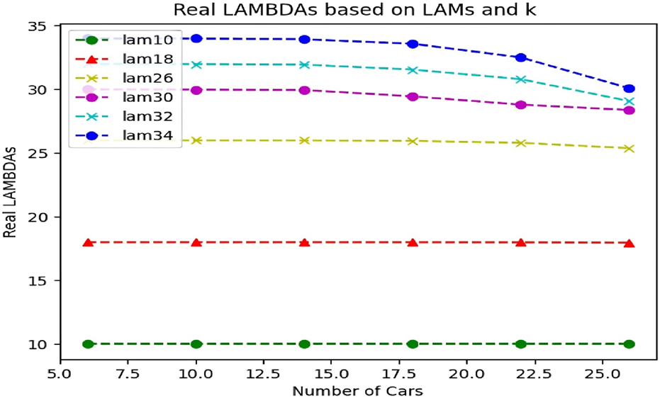
Actual lambda based on changes in P and input lambda.
4.1.3 Calculation of real lambda based on the simultaneous changes of input lambda and P
In the proposed model, we face a limited queue. Limited queue means that every request that comes to the vehicle is not necessarily placed in the queue, and this depends on the amount of queue filling.
If the queue is close to full, requests will most likely be dropped. This means that our input Lambda is not equal to the real Lambda due to the queue limit. Now, if we want to calculate the actual Lambda based on the input Lambda, we will reach Figure 12.
Figure 12 shows that the real Lambda of the network is greatly reduced at high values of the input Lambda, i.e. 30, 33, and 34, which are the threshold limit of not violating our condition. The reason for this is the limitation of the queue and the dropping of packets. Therefore, after a certain value of Lambda, the simultaneous increase of incoming Lambda and the possibility of sending it to RSU (P) leads to a decrease in network efficiency, and part of the requests are discarded. This graph shows that at p = 0.32, Lambda 30, 33, and 34 have almost the same output. Perhaps the reason for this can be analyzed in Figure 13. In Figure 13, where the probability of filling the queue is for the increase of the incoming number, we can see that the probability of filling the queue increases with the increase of requests entering the vehicle, due to the limit of the queue.
FIGURE 13
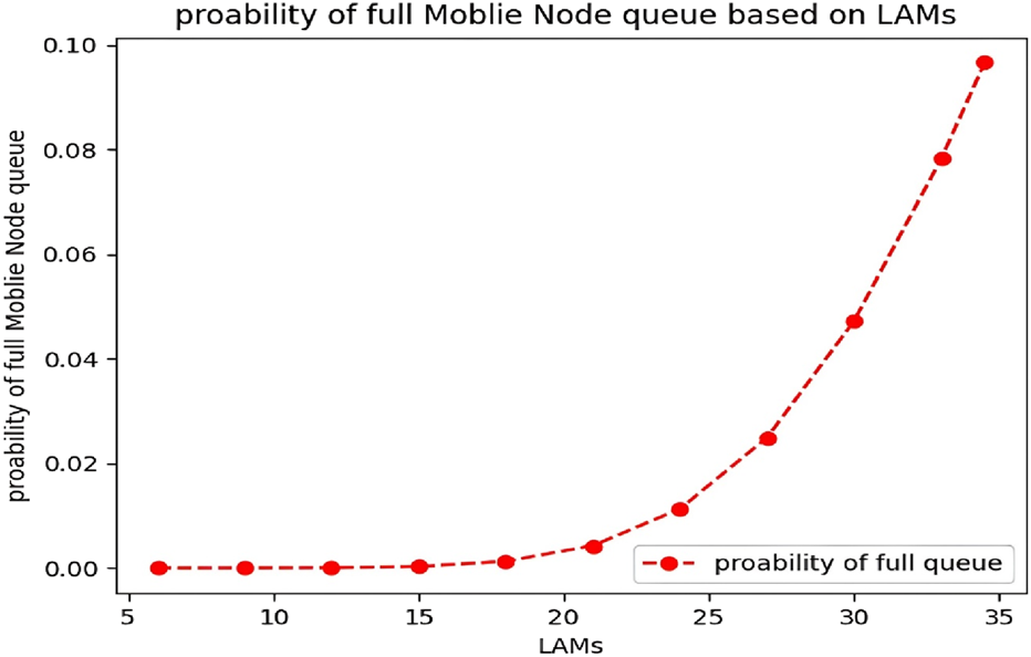
The probability of the vehicle queue filling up with the increase of incoming traffic.
Calculating the real Lambda using Formula 11 makes this problem more open.
4.1.4 Analysis of RSU queue changes due to lambda increase
When the probability of requests going to RSU increases, it means that we are facing an influx of data flow that, due to various reasons, such as Big Data or urgent requests, it is not possible to process them on mobile nodes. Therefore, it is sent to the upstream node or RSU.
In this part, we are trying to show the status of the queue in the RSU node by using the values in Table 6 and changing the input data.
TABLE 6
Analysis of condition ρ < 1 for RSU queue changes based on lambda changes.
First, we have to check that our condition about ρ < 1 is not violated. In the worst case, we check.
As can be seen in Figure 14, as expected, the state of the queue increases exponentially in proportion to the increase in Lambda, which indicates that the increase in Lambda along with the high variable p (probability of sending to RSU) leads to an increase in the length of the RSU queue.
FIGURE 14
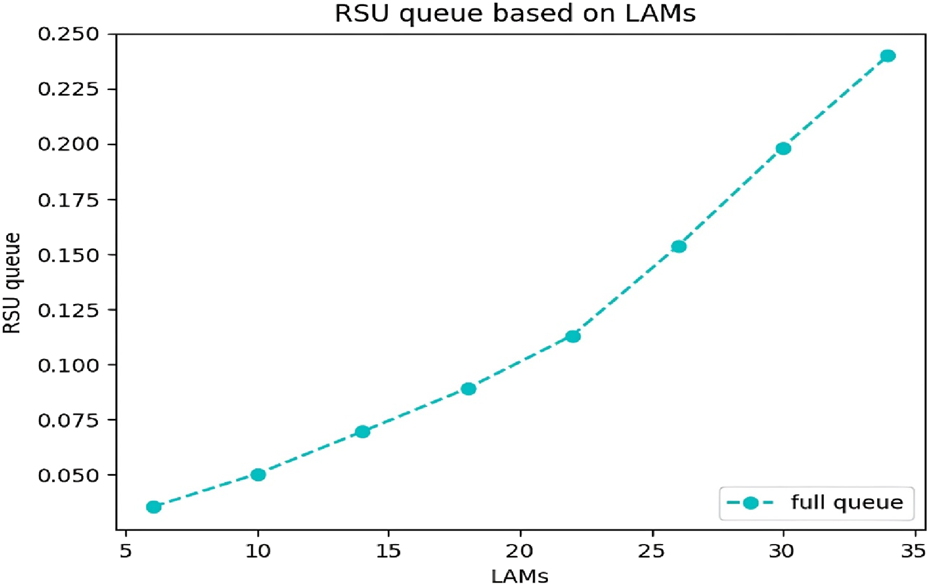
RSU Queuing based on incoming lambda changes.
4.1.5 Analysis of RSU queue with the simultaneous changes of lambda and k (number of vehicles)
Since we have considered the network in a steady state, by studying the behavior of this network in a long interval, we have reached an average of Lambda and Mayo (processing capacity) in the case of mobile nodes (vehicles), which determines the amount of request input and capacity. It is a process required by the vehicle. But in the real world, the density or in other words the number of vehicles is constantly changing. Therefore, this change in the number of vehicles can make significant changes in the entrance to the RSU. In the following, we will use the variable k to show the effect of this issue in the output of the calculations, and by changing its value while keeping other values constant, we will check the state of the RSU queue according to Table 7.
TABLE 7
Analysis of condition of ρ < 1 for RSU queue with lambda and k changes.
First, we have to check that our condition about ρ < 1 is not violated. In the worst case, we check:
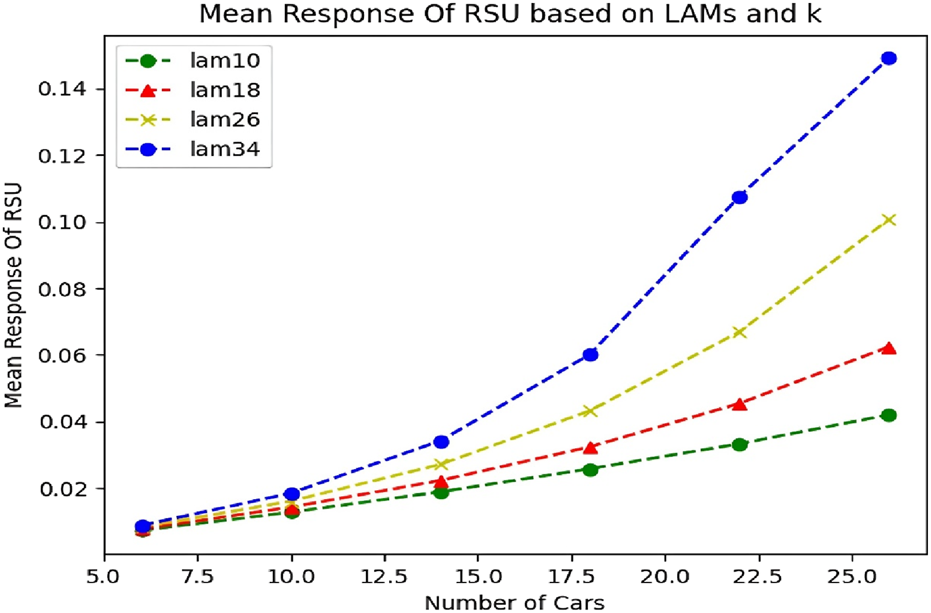
When we calculate the average response time graph of RSU with the same variables, we reach similar results. Figure 15 expresses the matter well.
FIGURE 15

The average RSU response time is based on the changes in the incoming traffic and the number of vehicles (k).
According to Figure 16, we can see that when the density of vehicles is low, the changes in the input Lambda have no effect on the average response time, and the graph grows linearly with a very low slope. But from k = 14 and in parallel with the increase of the input bandwidth, we see an exponential and significant growth of the response time.
FIGURE 16
Changes in the RSU queue are based on the changes in the incoming lambda and the number of vehicles (k).
The increasing trend of the queue against the changes of k is quite evident in the large Lambdas. Of course, this increase process will not last long due to the limited queue, and if we continue the current process under the condition of not violating the condition ρ < 1, we will see that the queue growth process will continue at a low speed. When the queue is about to fill up, requests are likely to be discarded. This means that our incoming Lambda is not a real Lambda due to the queue limit. Now, if we want to calculate the actual Lambda based on the input Lambda in proportion to the increase in the number of vehicles, we will reach Figure 17.
FIGURE 17
Real lambda RSU with simultaneous lambda and k changes.
4.1.6 Analysis of RSU queue with simultaneous lambda and P changes (probability of sending to RSU)
Here, we intend to Investigate the RSU queue while the variable P, which means the probability of sending to the RSU, changes at the same time as Lambda changes. We have made these calculations in Section 4.1.2 about the vehicle. Now, by recalculating this item in the case of RSU, we try to compare the results. We considered the values of the variables, as presented in Table 8. According to the procedure, we must first check that our condition about ρ < 1 is not violated:
TABLE 8
Analysis of condition ρ < 1 for RSU queue with lambda and P changes.
As can be seen in the diagram in Figure 18, as expected when the network or Lambda input and the probability of sending to RSU increases simultaneously, the number of JOBs in the RSU queue increases exponentially, especially in large Lambdas.
FIGURE 18
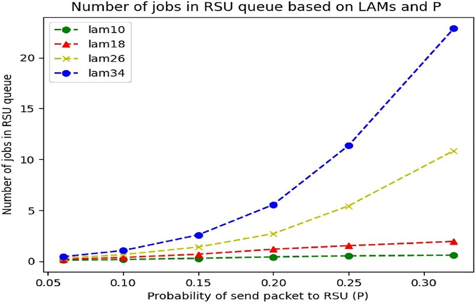
RSU queue with simultaneous lambda and P changes.
Now, we will calculate and check the average response time of RSU with the same parameters.
4.1.7 Calculation of the average response time in RSU according to the simultaneous change of lambda and P
As we can see in Figure 19, the results of calculating the response time are almost similar to the results of Figure 16. Something is clear at first sight at low values of the P variable (probability of sending requests to RSU), increasing the Lambda value does not affect RSU response time. So at p = 0.06, the response time in Lambda 10 is almost the same as in Lambda 34. But at higher values of P, we see a significant and exponential growth of the response time. One of the reasons for the effect of P changes in increasing the response time is that our queue is limited and as the probability of the package going to RSU increases, the RSU queue increases, and the formation of this queue leads to a delay in responding to requests. Another reason could be that as the package goes to RSU and as a result the RSU queue fills up, the probability of sending the package to the Cloud also increases, and this issue imposes a delay on the response time.
FIGURE 19
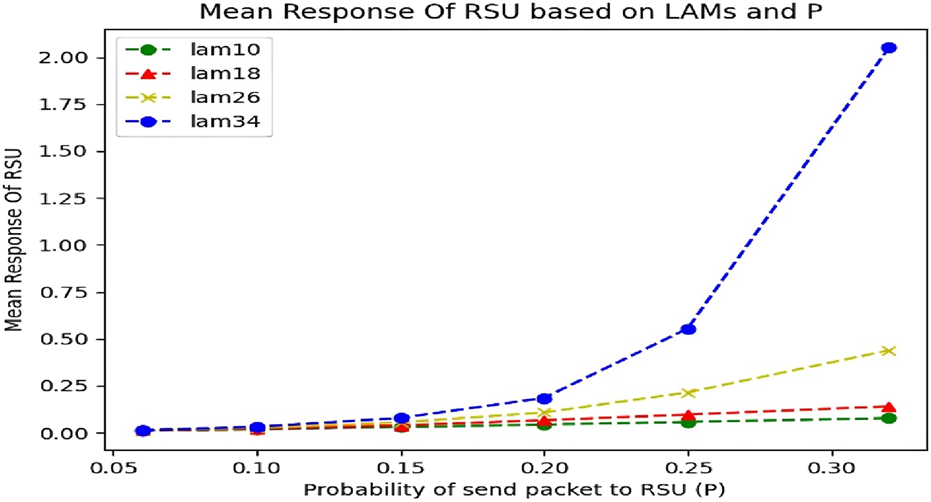
Mean response time of RSU with simultaneous changes of lambda and P.
4.1.8 Examining response time in cloud with simultaneous changes of q (probability of sending to cloud) and m (number of RSUs)
In our proposed model, due to the high processing resources of the vehicle and RSU, the Cloud is rarely involved in processing, and naturally, when the input request to the RSU is under certain conditions, such as the queue being full, as well as parameters such as the size of the packages (Job Size) and or requests with high processing urgency that are not in the processing power of RSU are sent to the Cloud, and since we usually have unlimited resources in the Cloud, we should not worry about the response time and the length of the Cloud queue in stable networks.
In this section, considering the processing capacity for Cloud (μc) and changes in the number of RSUs (variable m) and the probability of sending to Cloud (q) that affect the queue and response time of Cloud, we tried to show the queue status and response time in Cloud on the chart. In Table 9, the mentioned values are placed:
TABLE 9
| Variable | P | q | K | M | |||
|---|---|---|---|---|---|---|---|
| Value | 35 | 0.32 | 55 | 75 | 0.27 | 5 | 5 |
Adjusted parameters to analyze response time for cloud with q changes.
First, we must check that our condition about ρ < 1 is not violated:
The detailed numerical verification of the stability condition (ρ < 1) under different q values is summarized in Table 10.
TABLE 10
Analysis of condition ρ < 1 for response time in cloud with q changes.
Figure 20 shows the response time.
FIGURE 20
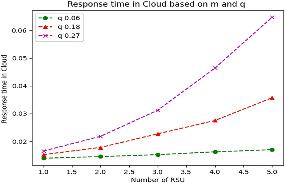
Cloud response time.
As we can see in Figure 20, as long as the variable q = 0.06 (green curve), the increase in the number of RSUs, which leads to an increase in the input data to the Cloud, does not have much effect on the response time of the Cloud. But with the simultaneous increase of q and RSU (m), the response time of Cloud increases significantly. The point that can be seen is that the response time increase of Cloud is dramatically intensified in larger q. This means that the increase in q and consequently the increase in request input to the Cloud causes the accumulation of JOBs ready to be processed and the formation of a queue based on the defined processing capacity of the Cloud, and after that, we will see an increase in the response time.
4.2 Analytical review and evaluation
The state of the art of the study was based on the topic of task offloading in vehicular networks and creating load balance in processing resources and the main idea of this research (Zhang et al., 2019). In this study, the problem of response time in vehicular networks was investigated with an algorithmic approach.
Using software-based networks, the authors have provided a solution based on load balancing in processing resources and compared their data with well-known algorithms in this field. Overall, the average response time of the vehicular network was improved with this solution. Now, in the continuation of this research, we are trying to mathematically show the average response time using the data of the study (Zhang et al., 2019) and make a comparison with each other.
In Figure 21, we can see the response time in the vehicular networks presented in (24).
FIGURE 21
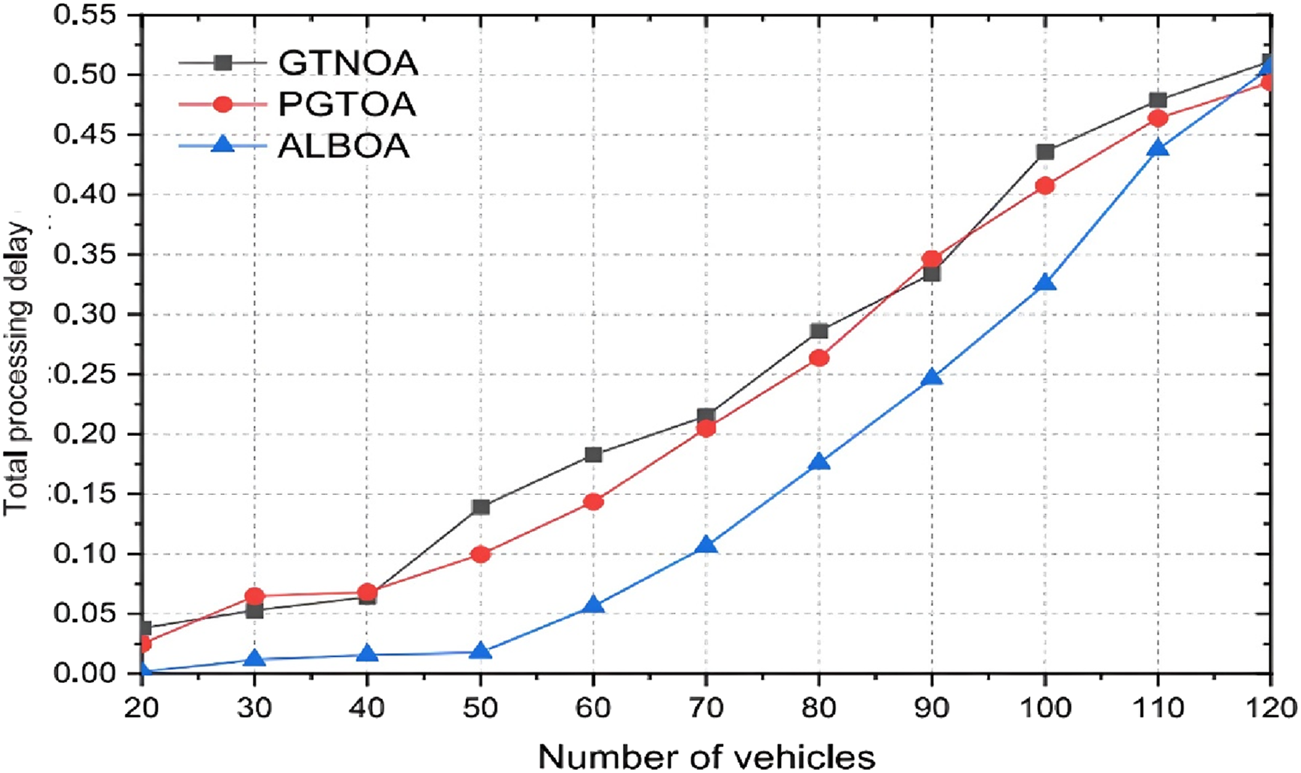
Average response time in vehicular networks based on the number of vehicles in the study (Zhang et al., 2019); time unit: seconds (s).
4.2.1 Analysis of average response time of the vehicular network based on the data of the article
We included the data of the study (Zhang et al., 2019) and then performed the relevant calculations, as shown in Table 11.
TABLE 11
| Variable | p | q | K | M | |||
|---|---|---|---|---|---|---|---|
| Value | 35 | 0.06 | 250 | 300 | 0.06 | 120 | 10 |
Dataset extracted from the base paper (Zhang et al., 2019).
First, we must check that our condition about ρ < 1 is not violated:
Table 12 presents the detailed analysis results for verifying ρ < 1 based on the dataset of Zhang et al. (2019).
As you can see in Figure 21, the blue graph shows the results of the work presented in the basic paper. A visual comparison of Figure 22 with the blue graph in Figure 20 shows that the mathematical calculation results of our study are close to the algorithmic method presented in the basic paper, which confirms the correctness of our calculation method. Therefore, it gives us the view that mathematical analysis, which is one of the fastest and least expensive analytical methods, at the same time works very close to accuracy and provides reliable outputs to us as analysts. The comparative performance results in terms of response time for both the base paper and our proposed model are summarized in Table 13. All reported response times in Figures 21, 22; Table 13 are in seconds (s).
FIGURE 22
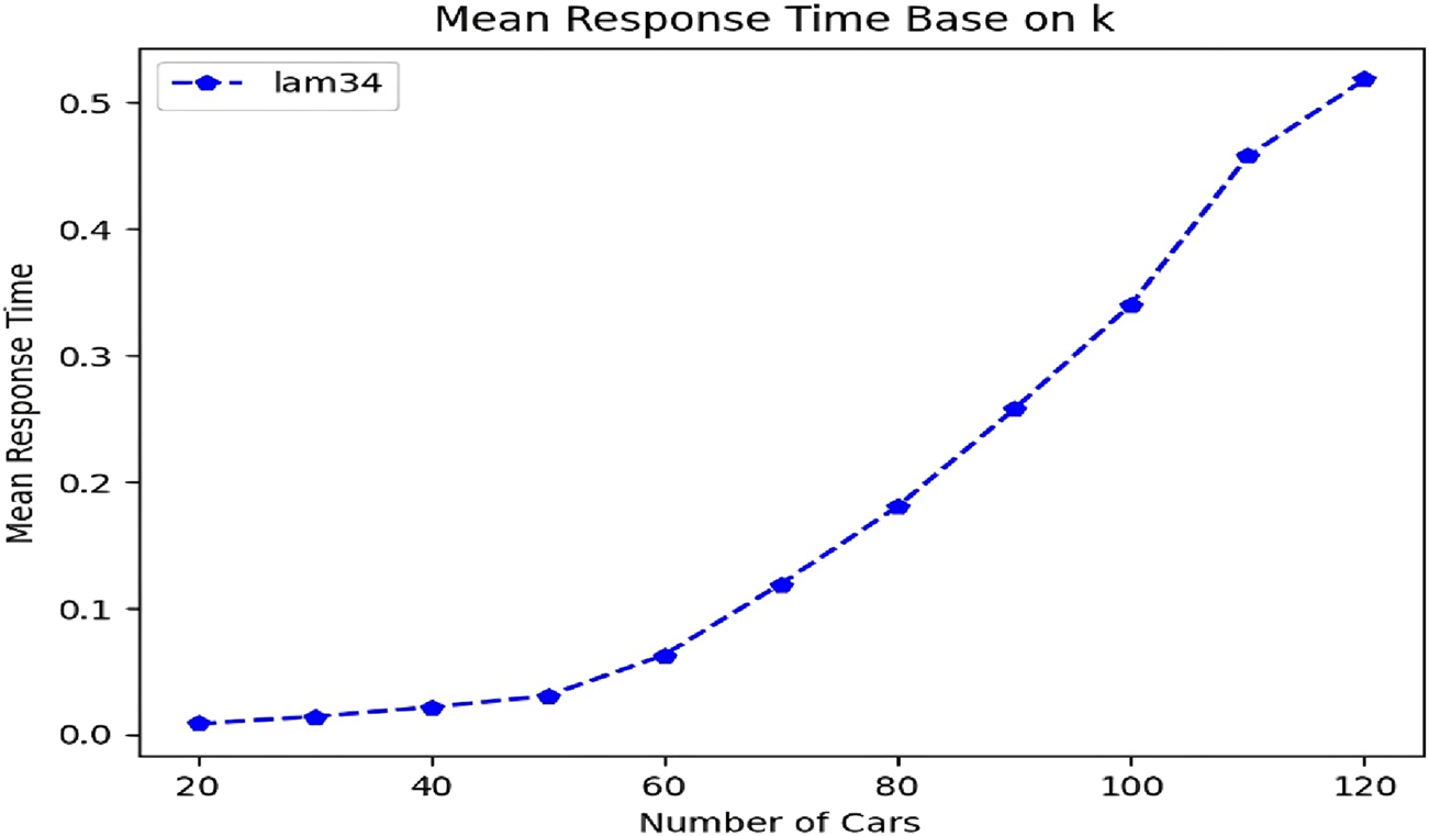
Average response time in vehicular networks based on the number of vehicles by mathematical analysis method of the study (Zhang et al., 2019); time unit: seconds (s).
TABLE 13
| N | 20 | 30 | 40 | 50 | 60 | 70 | 80 | 90 | 100 | 110 | 120 |
|---|---|---|---|---|---|---|---|---|---|---|---|
| Study | Response time (s) | ||||||||||
| Base Paper (24) | 0.019 | 0.021 | 0.023 | 0.025 | 0.051 | 0.105 | 0.176 | 0.253 | 0.323 | 0.431 | 0.482 |
| Our Study | 0.023 | 0.025 | 0.028 | 0.031 | 0.057 | 0.115 | 0.183 | 0.267 | 0.334 | 0.450 | 0.505 |
Comparative response time results of the base paper and our study for varying number of nodes (N).
4.3 Limitations and future research direction
Use of simple M/M/1 model with basic assumptions that may lead to insufficient accuracy in complex driving conditions.
Failure to consider traffic dynamics and real environmental conditions, including speed changes, variable traffic, and sudden obstacles.
Integrate real traffic data through reliable simulators and use more advanced models (such as G/G/k) to improve analytical accuracy.
Investigate the impact of dynamic parameters in driving scenarios and their relationship with changes in system resources.
5 Conclusion
From a scalability perspective, the SHARPE-based analytical evaluation solves steady-state probabilities of finite CTMCs via linear systems; computational cost grows roughly with the cube of the state-space size (O (n3)) for direct solvers, which is substantially lighter than packet-level simulation for comparable sweeps of system parameters.
In this study, we investigated the problem of response time in vehicular networks by using the rules governing mathematical calculations and the analytical method of Markov chains. By dividing the nodes in the network into three groups - mobile nodes (vehicles), roadside units (RSUs), and cloud - the average queue length for each group was calculated, and using Little’s Law, the average network response time was obtained. It was observed in the graphs that the response time of the vehicle increases linearly with the change in the density of nodes. However, due to the queue limitation, the input Lambda and the real Lambda were not identical to each other, which resulted in close response time values and a significant decrease in the slope of the response time graph.
The output of our work shows relatively similar results in the average network response time, indicating that we have achieved results close to those obtained from other expensive and time-consuming methods using the mathematical approach presented, which we considered an accomplishment in this paper. This confirms the correctness and accuracy of the mathematical analysis method and it shows that in addition to spending less time and money in the mathematical analysis method, we also obtain more reliable and accurate results. In the current paper, the main focus has been on theoretical analysis and system performance under controlled conditions. In this regard, real driving scenarios, which involve complex interactions between variables such as speed changes, inter-vehicle distance, and environmental conditions, have not been fully explored.
Additionally, the study does not account for real-world traffic dynamics and environmental factors, such as speed variations, fluctuating traffic, and unexpected obstacles.
We can also, in future work, examine other factors such as weather conditions and other possibilities affecting real-world driving conditions in more detail and include them in the final calculations.
Also, the routing of packets in a vehicular network can be investigated by mathematical analysis and Markov calculations and the results can be compared with other routing methods such as software-defined networks (SDN). We will Integrate real traffic data through reliable simulators and use more advanced models (such as G/G/k) to improve analytical accuracy. We will provide the impact of dynamic parameters in driving scenarios and their relationship with changes in system resources. We can also employ mathematical calculations in such a way that, in addition to ease of implementation, we can also try to improve the numerical results obtained with a new approach compared to other methods.
Statements
Data availability statement
The original contributions presented in the study are included in the article/supplementary material, further inquiries can be directed to the corresponding author.
Author contributions
MK: Writing – original draft, Data curation, Methodology, Conceptualization, Investigation, Software, Resources, Formal Analysis, Writing – review and editing. HR: Supervision, Writing – review and editing, Project administration. BKK: Writing – review and editing. SH: Writing – review and editing, Investigation. EA: Writing – review and editing. JHJ: Writing – original draft, Resources, Methodology, Validation, Writing – review and editing, Investigation. SG: Writing – review and editing, Investigation, Funding acquisition.
Funding
The author(s) declare that financial support was received for the research and/or publication of this article. This paper is financed by the European Union-NextGenerationEU, through the National Recovery and Resilience Plan of the Republic of Bulgaria, Project No. BG-RRP-2.004-0001-C01.
Conflict of interest
The authors declare that the research was conducted in the absence of any commercial or financial relationships that could be construed as a potential conflict of interest.
Generative AI statement
The author(s) declare that no Generative AI was used in the creation of this manuscript.
Any alternative text (alt text) provided alongside figures in this article has been generated by Frontiers with the support of artificial intelligence and reasonable efforts have been made to ensure accuracy, including review by the authors wherever possible. If you identify any issues, please contact us.
Publisher’s note
All claims expressed in this article are solely those of the authors and do not necessarily represent those of their affiliated organizations, or those of the publisher, the editors and the reviewers. Any product that may be evaluated in this article, or claim that may be made by its manufacturer, is not guaranteed or endorsed by the publisher.
Nomenclature
- MEC
Mobile Edge Computing
- VANET
Vehicular Ad hoc Network
- SHARPE
Symbolic Hierarchical Automated Reliability and Performance Evaluator
- CPU
Central Processing Unit
- VECN
Vehicular Edge Computing Networks
- CTMC
Continuous-Time Markov Chain
- DTMC
Discrete-Time Markov Chain
- SDN
Software Defined Network
- V2V
Vehicle-to-Vehicle
- RSU
Road Side Fixed Unit
References
1
Ansari N. Sun X. (2018). Mobile edge computing empowers internet of things. IEICE Trans. Commun.101 (3), 604–619. 10.1587/transcom.2017nri0001
2
Chao X. Pinedo M. (1999). Queueing networks: customers, signals, and product form solutions.
3
Dai Y. Xu D. Maharjan S. Zhang Y. (2018). Joint load balancing and offloading in vehicular edge computing and networks. IEEE Internet Things J.6 (3), 4377–4387. 10.1109/jiot.2018.2876298
4
Eiza M. H. Ni Q. Owens T. Min G. (2013). Investigation of routing reliability of vehicular ad hoc networks. EURASIP J. Wirel. Commun. Netw.2013, 179–15. 10.1186/1687-1499-2013-179
5
Gerla M. Kleinrock L. (2011). Vehicular networks and the future of the mobile internet. Comput. Netw.55 (2), 457–469. 10.1016/j.comnet.2010.10.015
6
Guo H. Liu J. (2018). Collaborative computation offloading for multiaccess edge computing over fiber–wireless networks. IEEE Trans. Veh. Technol.67 (5), 4514–4526. 10.1109/tvt.2018.2790421
7
Guo H. Liu J. Zhang J. Sun W. Kato N. (2018). Mobile-edge computation offloading for ultradense IoT networks. IEEE Internet Things J.5 (6), 4977–4988. 10.1109/jiot.2018.2838584
8
Hemmati A. Zarei M. Rahmani A. M. (2024). A systematic review of congestion control in internet of vehicles and vehicular ad hoc networks: techniques, challenges, and open issues. Int. J. Commun. Syst.37 (1), e5625. 10.1002/dac.5625
9
Huang C.-M. Chiang M.-S. Dao D.-T. Su W.-L. Xu S. Zhou H. (2018). V2V data offloading for cellular network based on the software defined network (SDN) inside mobile edge computing (MEC) architecture. IEEE Access6, 17741–17755. 10.1109/access.2018.2820679
10
Kanthasamy N. Wyglinski A. (2025). Framework for analyzing spatial interference in vehicle-to-vehicle communication networks with positional errors. Electronics14 (3), 510. 10.3390/electronics14030510
11
Lai Y.-C. Lin P. Liao W. Chen C.-M. (2010). A region-based clustering mechanism for channel access in vehicular ad hoc networks. IEEE J. Sel. Areas Commun.29 (1), 83–93. 10.1109/jsac.2011.110109
12
Liu T.-K. Silvester J. A. Polydoros A. (1995). “Performance evaluation of R-ALOHA in distributed packet radio networks with hard real-time communications,” in 1995 IEEE 45th Vehicular Technology Conference. Countdown to the Wireless Twenty-First Century, Chicago, IL, USA, 25-28 July 1995 (IEEE), 554–558.
13
Liu Y. Wang S. Huang J. Yang F. (2018). “A computation offloading algorithm based on game theory for vehicular edge networks,” in 2018 IEEE International Conference on Communications (ICC), Kansas City, MO, USA, 20-24 May 2018 (IEEE), 1–6.
14
Mao Y. You C. Zhang J. Huang K. Letaief K. B. (2017a). A survey on mobile edge computing: the communication perspective. IEEE Commun. Surv. and tutorials19 (4), 2322–2358. 10.1109/comst.2017.2745201
15
Mao Y. Zhang J. Song S. Letaief K. B. (2017b). Stochastic joint radio and computational resource management for multi-user mobile-edge computing systems. IEEE Trans. Wirel. Commun.16 (9), 5994–6009. 10.1109/twc.2017.2717986
16
Pang H. Wang Z. (2024). Dueling double deep Q network strategy in MEC for smart internet of vehicles edge computing networks. J. Grid Comput.22 (1), 37–12. 10.1007/s10723-024-09752-8
17
Quadar N. Chehri A. Debaque B. Ahmed I. Jeon G. (2024). Intrusion detection systems in automotive ethernet networks: challenges, opportunities and future research trends. IEEE Internet Things Mag.7 (2), 62–68. 10.1109/iotm.001.2300109
18
Rajkumar Y. Kumar S. S. (2024). An elliptic curve cryptography based certificate-less signature aggregation scheme for efficient authentication in vehicular ad hoc networks. Wirel. Netw.30 (1), 335–362. 10.1007/s11276-023-03473-8
19
Ram M. Kumar S. Kumar V. Sikandar A. Kharel R. (2019). Enabling green wireless sensor networks: energy efficient T-MAC using Markov chain based optimization. Electronics8 (5), 534. 10.3390/electronics8050534
20
Rider K. L. (1976). A simple approximation to the average queue size in the time-dependent M/M/1 queue. J. ACM (JACM).23 (2), 361–367. 10.1145/321941.321955
21
Rodrigues T. G. Suto K. Nishiyama H. Kato N. Temma K. (2018). Cloudlets activation scheme for scalable mobile edge computing with transmission power control and virtual machine migration. IEEE Trans. Comput.67 (9), 1287–1300. 10.1109/tc.2018.2818144
22
Sahu P. Kumar V. Gupta K. Prakash R. (2024). PMA-KDP: privacy-preserving mutual authentication and key distribution protocol in vehicular Ad-hoc networks (VANETs). Multimedia Tools Appl.83, 87505–87526. 10.1007/s11042-024-18754-3
23
Son S. Kwon D. Park Y. (2025). A seamless authentication scheme for edge-assisted internet of vehicles environments using chaotic maps. Electronics14 (4), 672. 10.3390/electronics14040672
24
Wang S. Zhang X. Zhang Y. Wang L. Yang J. Wang W. (2017). A survey on mobile edge networks: convergence of computing, caching and communications. Ieee Access5, 6757–6779. 10.1109/access.2017.2685434
25
Wu G. Li S. Wang S. Jiang Y. Li Z. (2019). Analysis and design of functional device for vehicular cloud computing. Electronics8 (5), 583. 10.3390/electronics8050583
26
Wu X. Dong S. Hu J. Huang Z. (2024). An efficient many-objective optimization algorithm for computation offloading in heterogeneous vehicular edge computing network. Simul. Model. Pract. Theory131, 102870. 10.1016/j.simpat.2023.102870
27
Yang Q. Lim A. Agrawal P. (2008). “Connectivity aware routing in vehicular networks,” in 2008 IEEE Wireless Communications and Networking Conference, Las Vegas, NV, USA, 31 March 2008 - 03 April 2008 (IEEE), 2218–2223.
28
Zhang J. Guo H. Liu J. Zhang Y. (2019). Task offloading in vehicular edge computing networks: a load-balancing solution. IEEE Trans. Veh. Technol.69 (2), 2092–2104. 10.1109/tvt.2019.2959410
Summary
Keywords
Markov chain, response time, performance evaluation, MEC, vehicular networks
Citation
Kalamati M, Raei H, Kumeda Kussia B, Hussain S, Arslan E, Hassannataj Joloudari J and Gaftandzhieva S (2025) Modeling and analysis of response time in vehicular networks using Markov chains. Front. Commun. Netw. 6:1657378. doi: 10.3389/frcmn.2025.1657378
Received
01 July 2025
Accepted
08 September 2025
Published
26 September 2025
Volume
6 - 2025
Edited by
P.K. Gupta, Jaypee University of Information Technology, India
Reviewed by
Ali Al-Allawee, University of Upper Alsace, France
Righa Tandon, Chitkara University, India
Updates
Copyright
© 2025 Kalamati, Raei, Kumeda Kussia, Hussain, Arslan, Hassannataj Joloudari and Gaftandzhieva.
This is an open-access article distributed under the terms of the Creative Commons Attribution License (CC BY). The use, distribution or reproduction in other forums is permitted, provided the original author(s) and the copyright owner(s) are credited and that the original publication in this journal is cited, in accordance with accepted academic practice. No use, distribution or reproduction is permitted which does not comply with these terms.
*Correspondence: Silvia Gaftandzhieva, sissiy88@uni-plovdiv.bg
Disclaimer
All claims expressed in this article are solely those of the authors and do not necessarily represent those of their affiliated organizations, or those of the publisher, the editors and the reviewers. Any product that may be evaluated in this article or claim that may be made by its manufacturer is not guaranteed or endorsed by the publisher.