Abstract
Machine learning techniques are being increasingly used in the analysis of clinical and omics data. This increase is primarily due to the advancements in Artificial intelligence (AI) and the build-up of health-related big data. In this paper we have aimed at estimating the likelihood of adverse drug reactions or events (ADRs) in the course of drug discovery using various machine learning methods. We have also described a novel machine learning-based framework for predicting the likelihood of ADRs. Our framework combines two distinct datasets, drug-induced gene expression profiles from Open TG–GATEs (Toxicogenomics Project–Genomics Assisted Toxicity Evaluation Systems) and ADR occurrence information from FAERS (FDA [Food and Drug Administration] Adverse Events Reporting System) database, and can be applied to many different ADRs. It incorporates data filtering and cleaning as well as feature selection and hyperparameters fine tuning. Using this framework with Deep Neural Networks (DNN), we built a total of 14 predictive models with a mean validation accuracy of 89.4%, indicating that our approach successfully and consistently predicted ADRs for a wide range of drugs. As case studies, we have investigated the performances of our prediction models in the context of Duodenal ulcer and Hepatitis fulminant, highlighting mechanistic insights into those ADRs. We have generated predictive models to help to assess the likelihood of ADRs in testing novel pharmaceutical compounds. We believe that our findings offer a promising approach for ADR prediction and will be useful for researchers in drug discovery.
1 Introduction
An adverse drug reaction (ADR) or event is defined as any unintended or undesired effect of a drug (Katzung et al., 2012; Coleman and Pontefract, 2016). ADRs are responsible for a high number of visits to emergency departments and in-hospital admissions. For instance, The Japan Adverse Drug Events (JADE) study reported around 17 adverse drug events per 1,000 patient days; 1.6% were fatal, 4.9% were life-threatening, and 33% were serious (Morimoto et al., 2010). These observations underscore the importance of toxicity assessment of any medication, especially in the early stages of drug discovery.
Machine learning methods can play a significant role in the interpretation of various data types to predict ADRs. These methods utilize multiple kinds of input data, such as chemical structures, gene expressions as well as text mining. These data types are then processed algorithmically with random forest (machine learning) or by an artificial neural network (deep learning) to generate prediction models. (Ho et al., 2016; Mayr et al., 2016; Gao et al., 2017; Zhang et al., 2017; Dana et al., 2018; Dey et al., 2018; Vamathevan et al., 2019).
Deep learning (Wang et al., 2020), a type of machine learning in Artificial intelligence (AI), has emerged as a promising and highly effective approach that can combine and interrogate diverse biological data types to generate new hypotheses. Deep learning is used extensively in the field of drug discovery and drug repurposing; however, its application in ADR prediction using gene expression data are rather limited.
Open TG–GATEs (Igarashi et al., 2014) is a large–scale toxicogenomics database that collects gene expression profiles of in vivo as well as in vitro samples that have been treated with various drugs. These expression profiles are an outcome of the Japanese Toxicogenomics Project (Uehara et al., 2009), which aimed to build an extensive database of drug toxicities for drug discovery. It also collects physiological, biochemical, and pathological measurements of the treated animals. Similar databases that aim to profile compound toxicities have also been developed (Chen et al., 2012; Alexander-Dann et al., 2018).
In contrast with other databases, such as (LINCS) (Subramanian et al., 2017), which have been used to predict multiple ADRs in a single study (Wang et al., 2016), Open TG–GATEs has been used to investigate individual/specific toxicities (Rueda-Zárate et al., 2017). To the best of our knowledge, no attempts have been made to provide a general framework for predicting multiple ADRs by using Open TG–GATEs.
The design of Open TG-Gates has several advantages over the LINCS database, chiefly the inclusion of in vivo samples with different doses and durations of administration. Therefore, we designed our analysis to encompass multiple samples with different dosages and duration for each compound, necessitating additional noise-removal steps in the data processing. This study describes our approach to generating deep learning-based, systematic ADR prediction models. This approach combines ADR occurrence data, including frequency details, from the FAERS (FDA Adverse Event Reporting System) database, with the gene expression profiles from Open TG-GATEs. We show how to improve the models’ performance by applying feature selection and hyperparameter optimization algorithms. The methodologies and models described in our study offer valuable tools for assessing the likelihood of ADRs in the course of drug discovery.
2 Materials and Methods
2.1 Overview
An overview of this study’s methodology is illustrated in Supplementary Figures S1, S2. First, we retrieved the relevant data from the above-described two databases (open TG–GATEs and FAERS). Next, we pre-processed the gene expression data to filter out noisy profiles by using a simple classification model, and retained only the significant ADR-drug associations (p < 0.05; Fisher’s exact test). Next, gene expression profile datasets were created by assigning positive and negative compounds for each ADR. We then split the datasets into training and validation sets three times. Subsequently, we used the training set data to perform feature selection and built deep neural network models with hyperparameter tuning using the Optuna package (see below). Finally, we evaluated the performances of the individual models on the validation set. We discuss these steps in detail below:
2.2 Data Retrieval and Processing
2.2.1 Open TG–GATEs Database
We extracted the in–vivo gene expression profiles of rat liver samples from the Open TG–GATEs database (Uehara et al., 2009; Igarashi et al., 2014). We selected the rat in–vivo data for our analysis chiefly because the in–vivo dataset included more compounds and a greater number of time points as compared with the in–vitro data (rat and human). However, our methodology can be easily extended to the other datasets.
This dataset was comprised of single-dose experiments and repeated-dose experiments. Single-dose experiments included administration-to-sacrifice periods of 3, 6, 9, or 24 h, whereas, in the repeated dose experiments, drugs were administered to rats once daily for 4, 8, 15, or 29 days. In the repeated-dose experiments, all rats were sacrificed 24 h after the last dose (Igarashi et al., 2014). In Open TG–GATEs, gene expression profiles were measured using Microarray technology (Affymetrix GeneChip).
The Affymetrix CEL files were downloaded from http://toxico.nibiohn.go.jp, and were preprocessed using the affy package (Gautier et al., 2004) from R Bioconductor (https://bioconductor.org/); Affymetrix Microarray Suite algorithm version 5 (mas5) was applied with the default parameters provided in affy, wherein normalization = TRUE. The resulting normalized dataset–hereafter referred to as “the raw dataset”–was used for all the subsequent analyses. Next, the fold change values were calculated for each probe set by dividing the raw dataset by the mean intensities of corresponding control samples; these values were then log2 transformed, hereafter referred to as the “log2FC dataset.”
Since the experimental design included multiple dosages and durations of exposure, the drugs had varied effects on the gene expression profiles. To reduce the noise, we predicted all the samples to be either treated or control using a generalized linear model with Lasso regularization [GLMNET package from R (Friedman et al., 2010)]. We used the whole raw dataset as the training set with a binary classification (treated and control). We fed through all the microarray data of the same duration to a single model, creating one model for each exposure set duration. Next, we estimated the probability of being classified as a treated sample for all the training sets. Only those samples with a probability of higher than 92% were included in our analysis. The remaining samples were considered to fall within the gray zone between treated and control, and they were discarded. We chose a cut-off of 92% because, at this threshold, no control samples were misclassified as treated.
2.2.2 Standardized FAERS Data
FAERS (FDA Adverse Event Reporting System) is “a database that collects adverse event reports, medication error reports, and product quality complaints resulting in adverse events that were submitted to FDA” (https://open.fda.gov/data/faers/). However, since the terms used in the FAERS database are left to the reporter to decide, inaccurate descriptions may often be incorporated, such as using general, vague terms to describe adverse events or treatments (Wong et al., 2015). To surmount this issue, we used the portion of the FAERS dataset standardized by Banda et al. (2016). They had curated and standardized the entries of the FAERS database for 11 years (2004–2015) following Medical Dictionary for Regulatory Activities (MedDRA) preferred terms (PT) (Wood, 1994).
We extracted all the compound-ADR combinations (70,553,900) from the total number of reports (4.8 million). Among the difficulties of using the FAERS database in ADRs prediction models is the presence of reports with multiple drugs used (Multipharma), which is expected in patients with chronic diseases. Such cases introduce unreliable associations added to the data noise. To solve this issue, we used only the associations in which the drug was assigned as the primary suspect (PS) (15,377,900). We calculated the number of reports for each compound-adverse drug event combination and calculated the total number of reports of the compound in question and also the total number of reports of the adverse event.
We assessed the significance of the compound-ADR associations by one-sided Fisher test (Ghosh, 1988) using “fisher.test” function from R with the parameter (alternative = “greater”). This option returns a significant p–value only in the event of a positive association, in contrast to “two.sides” test, which assesses both positive and negative associations Table 1.
TABLE 1
| Positive | Negative | Row total | |
|---|---|---|---|
| Compound | a | b | a + b |
| All other compounds | c | d | c + d |
| Column total | a + c | b + d | All reports |
Fisher exact test: a: the number of reports of that the compound cause the ADE, b: the number of reports of the compound that does not report the cause of ADE, c: the number of all positive reports of the ADE for all compounds other than the specific compound, e: the number of all negative reports of all compound other than the specific compound.
2.3 Model Building and Training
For a given ADR, we first designated the compounds with the most significant associations as positive compounds, (p–value threshold <0.05) and the least significantly associated compounds as negative compounds. In building a predictive model, we evenly balanced the number of positive and negative compounds, and retrieved the associated gene expression profiles (treated samples only as described above).
We then defined the training and validation sets by imposing two criteria: 1) the data-sets were balanced, i.e., the number of positive and negative samples were equal in both the sets, and; 2) no compounds were commonly shared between training and validation. The number of samples associated with individual compounds was highly variable, making it difficult to apply the standard cross-validation approach. To overcome this limitation, we shuffled the compounds between training and validation and sampled various training and validation set configurations. We then selected the most balanced configurations with training: validation ratios close to 80:20.
To prevent information leakage between the validation set and the training set, feature selection was performed using the training set only. Consequently, the validation set was used solely to identify the best performing models.
For feature selection, we used Boruta (Kursa and Rudnicki, 2010) implementation in Python https://github.com/scikit-learn-contrib/boruta_py, that is based on the random forest classifier from scikit-learn (Pedregosa et al., 2011) python package with default parameters. Important features (Huynh-Thu et al., 2012) are the variables (genes in this instance) that are essential to classify the samples as either positive or negative. Utilizing such key features for classification helps minimize data dimensionality. Moreover, these important features (genes) can offer deep insights into the biological phenomenon under study (the pathophysiology of the ADR in this study). To remove the effect of randomness and improve the accuracy of feature selection, Boruta generates additional shadow variables by shuffling the values of the original features, these additional shadow variables are added to the training set before assessing feature importance. Subsequently the importance of all the features is evaluated following the random forest algorithm, and the features with significantly higher significance than the shadow variables are considered important, while those with less importance are ignored. This procedure was repeated 100 times to detect the important features more accurately (Kursa and Rudnicki, 2010). Then, we used TensorFlow 2 (Abadi et al., 2016) to construct deep learning models. The input of the deep learning model is constructed of two-dimensional matrix with samples in rows and genes in columns.
Each model consists of three groups of layers, input, output, and hidden layers (Supplementary Figures S1, S2). We applied Optuna (Akiba et al., 2019) for hyperparameters tuning. Optuna uses the trial and error method for optimization, by randomly assigning values to the model hyperparameters from a range of values or choices offered by the user for a pre-determined number of trials. Subsequently, the results of all the trials can be examined to determine the optimal parameters. The parameters that were optimized included (Table 2): “depth”: corresponds to the number of densely connected layers (number of hidden layers aka DNN depth); the possible values are (1, 2, 5, 10, and 30). “width”: corresponds to the number of nodes per layer, the possible values were (100, 250, 500, and 700). To reduce the likelihood of over fitting, we used two measures. The first measure “drop” is to drop some nodes before going to the next layer. It took one of these values (0.2, 0.3, 0.4, and 0.5), (0.2 means 20% of nodes are dropped). The second measure is the introduction of noise: the value of introduced Gaussian noise (0.2, 0.3, 0.4, and 0.5). Other hyperparameters included: “activation”: corresponds to the activation function of the final layer (output layer); possible values: (“sigmoid,” “linear”), “learning rate” for Adam optimizer (Kingma and Ba, 2014) was selected among (0.001, 0.0005, and 0.00001). The models with the highest validation set accuracies were chosen.
TABLE 2
| Parameter | Choices |
|---|---|
| Depth | 1, 2, 5, 10, 30 |
| Width | 100, 250, 500, 700 |
| Drop percentage | 0.2, 0.3, 0.4, 0.7 |
| Gaussian noise | 0.2, 0.3, 0.4, 0.5 |
| Activation | Sigmoid, linear |
| Learning rate | 0.001, 0.0005, 0.00001 |
Optuna hyperparameter choices.
The maximum number of epochs was set at 800; however, we applied the “early stopping” strategy if the accuracy did not improve for 75 epochs. The best models were saved for each Optuna trial. The best parameters are shown in the Supplementary Table S1.
We opted not to employ the leave-p-out or k-fold cross-validation protocols to the gene expression samples because: 1) the training and validation sets should be assigned based on compound segregation, i.e., the same compound should not span training and validation sets, and 2) the number of samples differed from compound to compound and thus, creating balanced sets was impossible. We instead adopted the approach of creating three different training and validation sets. We also performed feature selection for each of the set combinations.
Overfitting is a significant issue in machine learning, especially if the amount of data is small. We attempted to minimize overfitting by combining multiple approaches; one such approach is early stopping, which stops the training when the model becomes more specific to the training set. We also used functions in TensorFlow and Keras that help generalize the models by dropping some nodes in the hidden layers by using the drop function and adding Gaussian noise in the deep layers. Table 2
2.4 Evaluation and Enrichment Analysis
Model performances were evaluated by testing the performance of the validation set prediction. We estimated the accuracy of the validation set and the area under the ROC (Receiver operating characteristic) curve using the scikit-learn (Pedregosa et al., 2011) package from Python.
TargetMine data analysis platform was used for enrichment analysis and gene annotation (Chen et al., 2019). Databases used for enrichment analysis were KEGG, Reactome, and NCI. p–values were calculated in TargetMine using one-tailed Fisher’s exact test. Multiple test correction was set to Benjamini Hochberg, with p-value significance threshold of 0.05.
3 Results
3.1 Data Processing
To reduce the data dispersion caused by multiple dose levels and administration durations (sacrifice period) in Open TG-GATEs, we filtered out low quality/unsuitable samples. To do that, we used Lasso to classify the samples to either treated or control classes. A total of 6,619 of 10,573 treated samples, chiefly belonging to the “Low” dose level category, were classified as controls and eventually excluded. Samples that were correctly classified as treated (3,953 samples) remained for subsequent analysis. (Table 3).
TABLE 3
| Original | Included | ||
|---|---|---|---|
| Dose level | Low | 3,540 | 421 |
| Middle | 3,537 | 1,212 | |
| High | 3,496 | 2,320 | |
| Sacrifice period | 24 h | 1,408 | 762 |
| 9 h | 1,371 | 556 | |
| 6 h | 1,371 | 533 | |
| 3 h | 1,368 | 518 | |
| 4 days | 1,275 | 254 | |
| 8 days | 1,275 | 472 | |
| 15 days | 1,266 | 500 | |
| 29 days | 1,239 | 358 |
The number of Open TG-GATEs samples included in the analysis after clustering using Lasso, dose level and sacrifice period details are shown.
3.2 Model Building and Training
We created a total of 14 models (Table 4). The number of compounds used to create each model ranged from 10 to 18. We equalized the number of positive compounds and negative compounds to generate balanced models.
TABLE 4
| ADR | Drugs | Samples | ||
|---|---|---|---|---|
| + | − | + | − | |
| AGEP | 5 | 5 | 203 | 87 |
| Bone marrow failure | 5 | 5 | 125 | 178 |
| Catatonia | 5 | 5 | 169 | 130 |
| Duodenal ulcer | 6 | 6 | 122 | 178 |
| ECG qt prolonged | 5 | 5 | 105 | 152 |
| Febrile neutropenia | 5 | 5 | 62 | 141 |
| Gastric haemorrhage | 5 | 5 | 124 | 161 |
| Hepatitis fulminant | 5 | 5 | 193 | 126 |
| Liver transplant | 9 | 9 | 297 | 244 |
| Lymphocytosis | 5 | 5 | 196 | 128 |
| Neutropenic sepsis | 6 | 6 | 89 | 165 |
| Optic atrophy | 6 | 6 | 122 | 139 |
| Torsade de pointes | 7 | 7 | 144 | 219 |
| Toxic epidermal necrolysis | 5 | 5 | 136 | 99 |
The number of compounds, and samples used to create ADRs prediction models. (AGEP: Acute generalized exanthematous pustulosis, ECG: Electrocardiogram). (+): Positive, (−): Negative.
3.3 Model Evaluation
The Average accuracy for all models was 89.94% (minimum = 71.42%, and maximum = 100%). The validation accuracies of the models are shown in Figure 1. The area under the Receiver Operating Characteristic (ROC) curve is shown in Figure 2. Matthews correlation coefficient (Matthews, 1975) of the predicted classes and the real classes for the modules are shown in Figure 3.
FIGURE 1
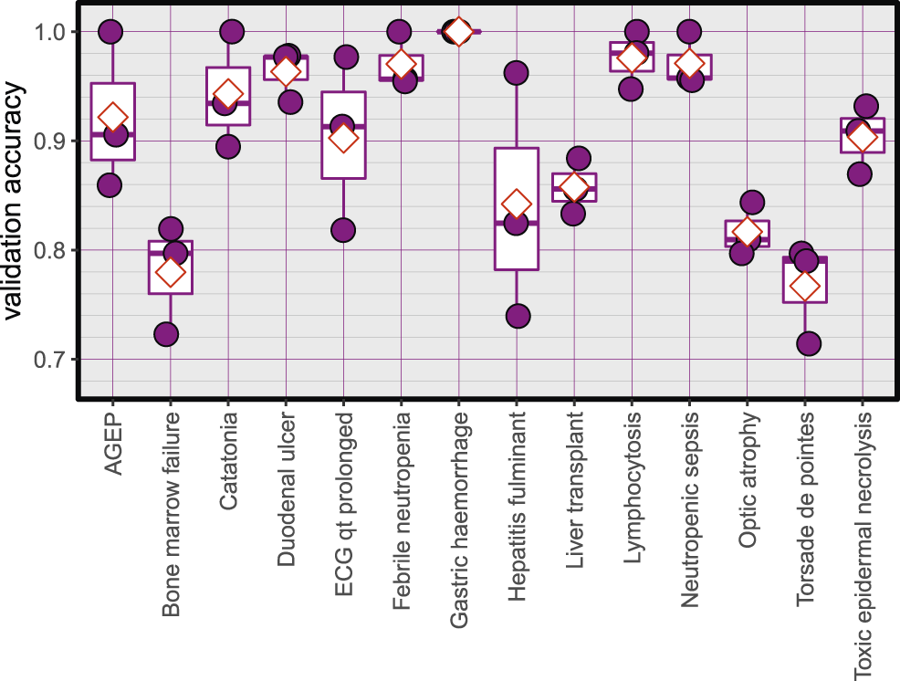
Validation accuracy of the created models, red diamonds represent the mean.
FIGURE 2
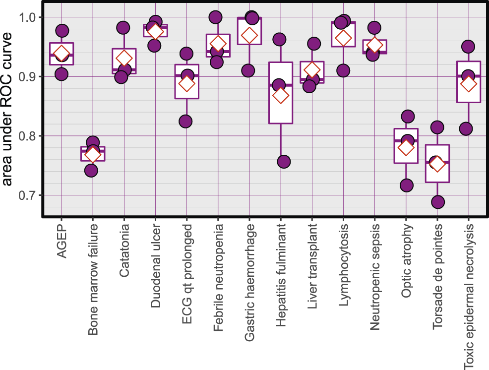
Area under ROC curves for the created models, red diamonds represent the mean.
FIGURE 3
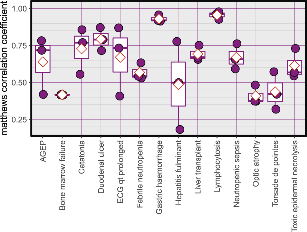
Matthews correlation coefficient, red diamonds represent the mean.
3.4 Case Study 1: Duodenal Ulcer
To highlight the effectiveness of our approach, we describe below our observations on the development of the duodenal ulcer ADR prediction model. Duodenal ulcer is a type of peptic ulcer disease characterized by the emergence of open sores on the duodenum’s inner lining of the duodenum (Kuna et al., 2019). It is mainly caused by the failure of gastrointestinal system inner coating protection, and the most common causing agents are Helicobacter Pylori infection and NSAIDs (Non-steroidal anti-inflammatory drugs). It can lead to serious bleeding or perforation.
3.4.1 Duodenal Ulcer Model Description
Using the FAERS database, the six most significantly associated drugs with duodenal ulcer were identified using Fisher test (positive drugs: Aspirin, Diclofenac, Ibuprofen, Indomethacin, Meloxicam, Naproxen) and the least associated drugs were also identified (negative drugs: Acetaminophen, Amiodarone, Bortezomib, Carbamazepine, Ciprofloxacin, Cyclophosphamide). Subsequently, the open TG–Gates samples of these drugs were used to build the prediction models. Details of the compounds used, the number of the gene expression samples associated with these compounds, and the results of the Fisher test (see Methods) are shown in Table 5. The ROC curves and the area under them for the three models of duodenal ulcer (each trained on a different training set) are shown in Figure 4 and the training curves are shown in Figure 5. The performance of these models showed that the area under the curve ranges from 0.94 to 0.99. The number of the features (genes) commonly selected among the three duodenal ulcer models were 108.
TABLE 5
| Fisher (p) | No | Class | |
|---|---|---|---|
| Acetaminophen | 4.88 × 10⁻¹ | 50 | Negative |
| Amiodarone | 9.35 × 10⁻¹ | 31 | Negative |
| Aspirin | 4.67 × 10−233 | 45 | Positive |
| Bortezomib | 3.57 × 10⁻¹ | 24 | Negative |
| Carbamazepine | 9.99 × 10⁻¹ | 45 | Negative |
| Ciprofloxacin | 9.67 × 10⁻¹ | 7 | Negative |
| Cyclophosphamide | 8.29 × 10⁻¹ | 21 | Negative |
| Diclofenac | 1.3 × 10−66 | 9 | Positive |
| Ibuprofen | 1.22 × 10−112 | 24 | Positive |
| Indomethacin | 5.40 × 10⁻¹⁵ | 12 | Positive |
| Meloxicam | 2.15 × 10⁻³⁵ | 10 | Positive |
| Naproxen | 2.02 × 10−78 | 22 | Positive |
Details of the data set for the duodenal ulcer model (compounds, the number of the samples, the p-value of the Fisher test and the class in the training or test sets). Positive class compounds are those that can cause doudenal ulcer, while Negative class compounds are controls. Entries were ordered alphabetically.
FIGURE 4
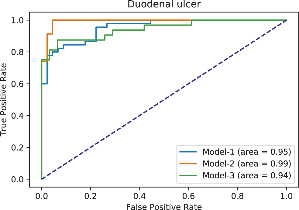
Area under ROC curves for duodenal ulcer models. Each color corresponds to a different model.
FIGURE 5
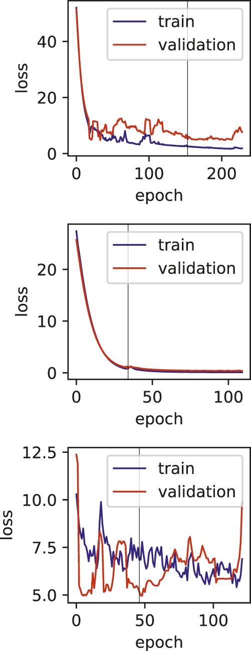
Training and validation loss plots for Duodenal ulcer models, vertical line marks the early stopping.
3.4.2 Enrichment Analysis
Pathway enrichment analysis (see Methods) using the duodenal ulcer-selected features (Supplementary Table S2) clearly highlighted the involvement of bleeding cascade and complement function (Table 6).
TABLE 6
| Pathway | P value |
|---|---|
| Complement and coagulation cascades (rno04610) | 1.86 × 10⁻¹¹ |
| Regulation of Complement cascade (R-RNO-977606) | 1.56 × 10⁻⁵ |
| Complement cascade (R-RNO-166658) | 9.16 × 10⁻⁵ |
| Pertussis (rno05133) | 3.84 × 10⁻³ |
| Fatty acid degradation (rno00071) | 4.83 × 10⁻³ |
The enrichment analysis results of duodenal ulcer model, showing the involvement of both complement and coagulation functions.
The manifestation of a duodenal ulcer activates the complement cascade, which is probably due to the inflammation caused by the acid effect on the intestinal mucosa. Bleeding is also linked with the duodenal ulcer disease. The enrichment of the Fatty acid degradation pathway is consistent with the fact that the majority of the compounds that cause duodenal ulcers are NSAIDs that inhibit Arachidonic acid metabolism, which is a part of the Fatty acid metabolism pathway.
3.5 Case Study 2: Hepatitis Fulminant
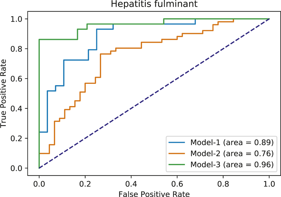
From FAERS database, the five most significantly associated drugs with hepatitis fulminant (Morabito and Adebayo, 2014; Bernal and Wendon, 2013) were identified using Fisher test (positive drugs: danazol, famotidine, flutamide, mexiletine, ticlopidine) and the least associated drugs were also identified (negative drugs: carbamazepine, ciprofloxacine, ibuprofen, naproxen, simvastatin). Subsequently, the open TG–Gates samples of these drugs were used to build the prediction models. Details of the compounds used, the number of the gene expression samples associated with these compounds, and the results of the Fisher test (see Methods) are shown in Table 7. The ROC curves and the area under them for the three models of hepatitis fulminant (each trained on a different training set) are shown in Figure 6 as well as training curves in Figure 7. The performance of these models showed that the area under the curve ranges from 0.76 to 0.96. The number of the features (genes) commonly selected among the three hepatitis fulminant models were 108. Pathway enrichment analysis using the hepatitis fulminant-selected features (Supplementary Table S2) clearly highlighted the involvement of Activation of NF-kappaB in B cells and Ub-specific processing proteases (Table 8), which coincides with the previous publications that suggest NF-kappaB pathway is linked to liver pathologies, including viral hepatitis, fibrosis and liver necrosis (Sun and Karin, 2008).
TABLE 7
| Fisher (p) | No | Class | |
|---|---|---|---|
| Carbamazepine | 7.72 × 10⁻² | 45 | Negative |
| Ciprofloxacin | 2.23 × 10⁻¹ | 7 | Negative |
| Danazol | 5.92 × 10⁻⁴ | 51 | Positive |
| Famotidine | 6.63 × 10⁻¹⁶ | 11 | Positive |
| Flutamide | 1.02 × 10⁻⁵ | 45 | Positive |
| Ibuprofen | 6.66 × 10⁻¹ | 24 | Negative |
| Mexiletine | 1.41 × 10⁻⁵ | 29 | Positive |
| Naproxen | 9.79 × 10⁻¹ | 22 | Negative |
| Simvastatin | 2.42 × 10⁻¹ | 28 | Negative |
| Ticlopidine | 1.78 × 10⁻⁶ | 57 | Positive |
Details of the data set for the hepatits fulminant model (compounds, the number of the samples, the p-value of the Fisher test and the class in the training or test sets). Positive class compounds are those that can cause hepatitis fulminant, while Negative class compounds are controls. Entries were ordered alphabetically.
FIGURE 6
Area under ROC curves for hepatitis fulminant models. Each color corresponds to a different model.
FIGURE 7
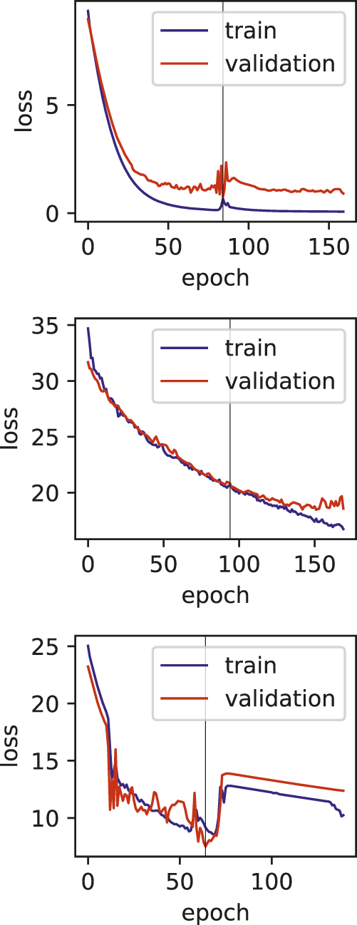
Training and validation loss plots for hepatitis fulminant models, vertical line marks the early stopping.
TABLE 8
| Pathway | P value |
|---|---|
| Biological oxidations (computationally inferred) (R-RNO-211859) | 0.0001398 |
| Metabolism of xenobiotics by cytochrome P450 (rno00980) | 0.0004514 |
| Phase II - Conjugation of compounds (computationally inferred) (R-RNO-156580) | 0.0004669 |
| Metabolism (computationally inferred) (R-RNO-1430728) | 0.0058958 |
| Activation of NF-kappaB in B cells (computationally inferred) (R-RNO-1169091) | 0.0078192 |
| Ub-specific processing proteases (computationally inferred) (R-RNO-5689880) | 0.0089848 |
The enrichment analysis results of hepatitis fulminant model (Top pathways).
4 Discussion
We have described a novel approach that combined toxicogenomics gene expression profiles extracted from Open TG-GATEs and ADRs reports extracted from FAERS to predict the likelihood of ADRs. This integration of two highly distinct data types allowed us to predict ADRs successfully. Moreover, it led to creating a novel dataset that associated drug-induced gene expression profiles with ADRs.
To overcome the significant challenges in combining the two datasets, we first sought to extract the individual drug-induced gene expression signature from Open TG-GATEs. Next, we extracted the ADR occurrence frequencies for these drugs and estimated their statistical significance to eventually combine the two datasets.
Moreover, due to multiple dose-levels and sacrifice periods and the presence of repeated and single administration events, the drug-induced gene expression profiles were fairly noisy. We generated a simple model to classify all the samples as either control or treated classes using Lasso to filter out this noise. We performed a rigorous statistical assessment to narrow down suitable samples for subsequent analyses (see Methods for details).
Recently, deep learning has gathered an increasing usage in the field of drug discovery (Eduati et al., 2015; Mayr et al., 2016; Preuer et al., 2017; Zhang et al., 2017; Dey et al., 2018; Lee and Chen, 2019). In this study we have used deep learning together with feature selection to reduce the data dimensionality and avoid overfitting due to limited samples.
Previously, Wang et al. (2016) utilized multiple cell lines to develop predictive models for multiple ADRs. Another study (Joseph et al., 2013) demonstrated that blood transcriptomics could be used to examine other organ toxicities. Our results have supported this notion by exhibiting robust prediction models with high accuracy using liver samples. Liver is a vital organ for drug metabolism and receives a significant amount of blood, and hence, it is widely used in drug toxicity studies. Moreover, even in the absence of pathological responses to the compound toxicity, cells still display differences in gene expression profiles.
This study utilized in vivo gene expression data in contrast with another study (Wang et al., 2016) that utilized the data from the LINCS database (Subramanian et al., 2017), a collection of in vitro gene expression profiles from human cell lines. Our approach is easily applicable to other publicly available collections of toxicogenomics data, such as those from Drug Matrix (Svoboda et al., 2019). Another difference is that Wang et al. (2016) combined chemical structure and Gene Ontology (GO) term associations in their models. They also selected only a single gene expression profile to represent the compound effects; in contrast, our method analyzed multiple samples with different doses and durations of each compound’s exposure. Hence, our method is better equipped to account for the biological variations that are inherent in drug-induced physiological and phenotypic responses. Indeed, our models performed better than Wang et al.’s gene expression data-only models (Wang et al., 2016). This difference in performances may be attributed to our utilization of multiple samples for each compound.
Studies related to specific ADR or systems examined in this study have been recently published. Liu et al. (2020) investigated the prediction of drug-induced liver injury utilizing data from different sources and showed comparable accuracy to ours. The highest AUC of their created models was around 0.86. However, their approach is specific to drug-induced liver injury. They also utilized chemical structures and protein-related information, among many other data types. Similarly, Ben Guebila and Thiele (2019) predicted Gastric ulcers using gene expression data from the LINCS database with an AUC of 0.97. They also compared using gene expression alone with adding more information to the same model.
Using the Optuna optimization package (Akiba et al., 2019) made our prediction models’ creation computationally expensive; hence, only a limited number of models were built. However, our approach can help generate models to serve specific applications using other data resources such as DrugMatrix, depending on the user’s needs.
One of the limitations of this study is the relatively smaller number of samples, and also the various dosages and durations of the exposure to the drugs. The effect of these limitations can be seen in the training plots (Figures 5, 7), which show fluctuating curves. Accordingly, a few models display lower correlations with ADR prediction as evidenced from their Matthews correlation coefficient plots (Figure 3), however, the majority have correlation values greater than 50%.
In conclusion, we have developed 14 deep learning models to predict adverse drug events utilizing the publicly available Open TG–Gates and FAERS databases. These models can be used to examine if a new drug candidate can cause these side effects. Moreover, following the same feature selection and model building and tuning steps, other models can be created for other ADRs.
Statements
Data availability statement
The prediction models and auxiliary information associated with this study are available at: https://github.com/attayeb/adr
Author contributions
AM, and KM: concept, design and draft writing. AM: data analysis, models building, AM, LT, and KM: results analysis, and manuscript writing. All authors contributed to the article and approved the submitted version.
Acknowledgments
We would like to gratefully acknowledge Dr. Yoshinobu Igarashi (Laboratory of Toxicogenomics Informatics, NIBIOHN) for his valuable suggestions and comments. The statements made here are solely the responsibility of the authors.
Conflict of interest
The authors declare that the research was conducted in the absence of any commercial or financial relationships that could be construed as a potential conflict of interest.
Publisher’s note
All claims expressed in this article are solely those of the authors and do not necessarily represent those of their affiliated organizations, or those of the publisher, the editors and the reviewers. Any product that may be evaluated in this article, or claim that may be made by its manufacturer, is not guaranteed or endorsed by the publisher.
Supplementary material
The Supplementary Material for this article can be found online at: https://www.frontiersin.org/articles/10.3389/fddsv.2021.768792/full#supplementary-material
References
1
Abadi M. Agarwal A. Barham P. Brevdo E. Chen Z. Citro C. et al (2016). Tensorflow: Large-Scale Machine Learning on Heterogeneous Distributed Systems. arXiv preprint 1603.04467.
2
Akiba T. Sano S. Yanase T. Ohta T. Koyama M. (2019). Optuna: A next-generation hyperparameter optimization framework. In Proceedings of the 25th ACM SIGKDD international conference on knowledge discovery and data mining. 2623-2631. doi: 10.1145/3292500.3330701.
3
Alexander-Dann B. Pruteanu L. L. Oerton E. Sharma N. Berindan-Neagoe I. Módos D. et al (2018). Developments in Toxicogenomics: Understanding and Predicting Compound-Induced Toxicity from Gene Expression Data. Mol. Omics14, 218–236. 10.1039/c8mo00042e
4
Banda J. M. Evans L. Vanguri R. S. Tatonetti N. P. Ryan P. B. Shah N. H. (2016). A Curated and Standardized Adverse Drug Event Resource to Accelerate Drug Safety Research. Sci. Data3. 10.1038/sdata.2016.26
5
Ben Guebila M. Thiele I. (2019). Predicting Gastrointestinal Drug Effects Using Contextualized Metabolic Models. Plos Comput. Biol.15, e1007100. 10.1371/journal.pcbi.1007100
6
Bernal W. Wendon J. (2013). Acute Liver Failure. N. Engl. J. Med.369, 2525–2534.
7
Chen M. Zhang M. Borlak J. Tong W. (2012). A Decade of Toxicogenomic Research and its Contribution to Toxicological Science. Toxicol. Sci.130, 217–228. 10.1093/toxsci/kfs223
8
Chen Y.-A. Tripathi L. P. Fujiwara T. Kameyama T. Itoh M. N. Mizuguchi K. (2019). The TargetMine Data Warehouse: Enhancement and Updates. Front. Genet.10. 10.3389/fgene.2019.00934
9
Coleman J. J. Pontefract S. K. (2016). Adverse Drug Reactions. Clin. Med.16, 481–485. 10.7861/clinmedicine.16-5-481
10
Dana D. Gadhiya S. St. Surin L. Li D. Naaz F. Ali Q. et al (2018). Deep Learning in Drug Discovery and Medicine; Scratching the Surface. Molecules23, 2384. 10.3390/molecules23092384
11
Dey S. Luo H. Fokoue A. Hu J. Zhang P. (2018). Predicting Adverse Drug Reactions through Interpretable Deep Learning Framework. BMC Bioinformatics19. 10.1186/s12859-018-2544-0
12
Eduati F. Mangravite L. M. Mangravite L. M. Wang T. Tang H. Bare J. C. et al (2015). Prediction of Human Population Responses to Toxic Compounds by a Collaborative Competition. Nat. Biotechnol.33, 933–940. 10.1038/nbt.3299
13
Friedman J. Hastie T. Tibshirani R. (2010). Regularization Paths for Generalized Linear Models via Coordinate Descent. J. Stat. Softw.33, 1–22. 10.18637/jss.v033.i01
14
Gao M. Igata H. Takeuchi A. Sato K. Ikegaya Y. (2017). Machine Learning-Based Prediction of Adverse Drug Effects: An Example of Seizure-Inducing Compounds. J. Pharmacol. Sci.133, 70–78. 10.1016/j.jphs.2017.01.003
15
Gautier L. Cope L. Bolstad B. M. Irizarry R. A. (2004). affy--analysis of Affymetrix GeneChip Data at the Probe Level. Bioinformatics20, 307–315. 10.1093/bioinformatics/btg405
16
Ghosh J. K. (1988). A Discussion on the fisher Exact Test. Statistical Information and Likelihood. New York: Springer, 321–324. 10.1007/978-1-4612-3894-2_18A Discussion on the Fisher Exact Test
17
Ho T.-B. Le L. Tran Thai D. Taewijit S. (2016). Data-driven Approach to Detect and Predict Adverse Drug Reactions. Cpd22, 3498–3526. 10.2174/1381612822666160509125047
18
Huynh-Thu V. A. Saeys Y. Wehenkel L. Geurts P. (2012). Statistical Interpretation of Machine Learning-Based Feature Importance Scores for Biomarker Discovery. Bioinformatics28, 1766–1774. 10.1093/bioinformatics/bts238
19
Igarashi Y. Nakatsu N. Yamashita T. Ono A. Ohno Y. Urushidani T. et al (2014). Open TG-GATEs: a Large-Scale Toxicogenomics Database. Nucleic Acids Res.43, D921–D927. 10.1093/nar/gku955
20
Joseph P. Umbright C. Sellamuthu R. (2013). Blood Transcriptomics: Applications in Toxicology. J. Appl. Toxicol., a–n. 10.1002/jat.2861
21
Katzung B. G. (2012). “Development & Regulation of Drugs,” in Basic & Clinical Pharmacology. Editors KatzungB. G.MastersS. B.TrevorA. J. (New York: McGraw-Hill), 69–78. chap. 5.
22
Kingma D. P. Ba J. (2014). Adam: A method for stochastic optimization. arXiv preprint: 1412.6980.
23
Kuna L. Jakab J. Smolic R. Raguz-Lucic N. Vcev A. Smolic M. (2019). Peptic Ulcer Disease: A Brief Review of Conventional Therapy and Herbal Treatment Options. Jcm8, 179. 10.3390/jcm8020179
24
Kursa M. B. Rudnicki W. R. (2010). Feature Selection with theBorutaPackage. J. Stat. Soft.36. 10.18637/jss.v036.i11
25
Lee C. Y. Chen Y.-P. P. (2019). Machine Learning on Adverse Drug Reactions for Pharmacovigilance. Drug Discov. Today24, 1332–1343. 10.1016/j.drudis.2019.03.003
26
Liu X. Zheng D. Zhong Y. Xia Z. Luo H. Weng Z. (2020). Machine-learning Prediction of Oral Drug-Induced Liver Injury (DILI) via Multiple Features and Endpoints. Biomed. Res. Int.2020, 1–10. 10.1155/2020/4795140
27
Matthews B. W. (1975). Comparison of the Predicted and Observed Secondary Structure of T4 Phage Lysozyme. Biochim. Biophys. Acta (Bba) - Protein Struct.405, 442–451. 10.1016/0005-2795(75)90109-9
28
Mayr A. Klambauer G. Unterthiner T. Hochreiter S. (2016). DeepTox: Toxicity Prediction Using Deep Learning. Front. Environ. Sci.3. 10.3389/fenvs.2015.00080
29
Mohsen A. Tripathi L. P. Mizuguchi K. (2020). Deep Learning Prediction of Adverse Drug Reactions Using Open TG-GATEs and FAERS Databases. arXiv preprint: 2010.05411.
30
Morabito V. Adebayo D. (2014). Fulminant Hepatitis: Definitions, Causes and Management. Health, 2014. 10.4236/health.2014.610130
31
Morimoto T. Sakuma M. Matsui K. Kuramoto N. Toshiro J. Murakami J. et al (2010). Incidence of Adverse Drug Events and Medication Errors in japan: the JADE Study. J. Gen. Intern. Med.26, 148–153. 10.1007/s11606-010-1518-3
32
Pedregosa F. Varoquaux G. Gramfort A. Michel V. Thirion B. Grisel O. et al (2011). Scikit-learn: Machine Learning in python. J. Machine Learn. Res.12, 2825–2830.
33
Preuer K. Lewis R. P. I. Hochreiter S. Bender A. Bulusu K. C. Klambauer G. (2017). DeepSynergy: Predicting Anti-cancer Drug Synergy with Deep Learning. Bioinformatics34, 1538–1546. 10.1093/bioinformatics/btx806
34
Rueda-Zárate H. A. Imaz-Rosshandler I. Cárdenas-Ovando R. A. Castillo-Fernández J. E. Noguez-Monroy J. Rangel-Escareño C. (2017). A Computational Toxicogenomics Approach Identifies a List of Highly Hepatotoxic Compounds from a Large Microarray Database. PLOS ONE12, e0176284. 10.1371/journal.pone.0176284
35
Subramanian A. Narayan R. Corsello S. M. Peck D. D. Natoli T. E. Lu X. et al (2017). A Next Generation Connectivity Map: L1000 Platform and the First 1,000,000 Profiles. Cell171, 1437–1452. 10.1016/j.cell.2017.10.049
36
Sun B. Karin M. (2008). NF-κB Signaling, Liver Disease and Hepatoprotective Agents. Oncogene27, 6228–6244. 10.1038/onc.2008.300
37
Svoboda D. L. Saddler T. Auerbach S. S. (2019).An Overview of National Toxicology Program's Toxicogenomic Applications: DrugMatrix and ToxFX. In Advances in Computational Toxicology. Springer, 141–157. 10.1007/978-3-030-16443-0_8
38
Uehara T. Ono A. Maruyama T. Kato I. Yamada H. Ohno Y. et al (2009). The Japanese Toxicogenomics Project: Application of Toxicogenomics. Mol. Nutr. Food Res.54, 218–227. 10.1002/mnfr.200900169
39
Vamathevan J. Clark D. Czodrowski P. Dunham I. Ferran E. Lee G. et al (2019). Applications of Machine Learning in Drug Discovery and Development. Nat. Rev. Drug Discov.18, 463–477. 10.1038/s41573-019-0024-5
40
Wang X. Zhao Y. Pourpanah F. (2020). Recent Advances in Deep Learning. Int. J. Mach. Learn. Cyber.11, 747–750. 10.1007/s13042-020-01096-5
41
Wang Z. Clark N. R. Ma’ayan A. (2016). Drug-induced Adverse Events Prediction with the LINCS L1000 Data. Bioinformatics32, 2338–2345. 10.1093/bioinformatics/btw168
42
Wong C. K. Ho S. S. Saini B. Hibbs D. E. Fois R. A. (2015). Standardisation of the FAERS Database: a Systematic Approach to Manually Recoding Drug Name Variants. Pharmacoepidemiol. Drug Saf.24, 731–737. 10.1002/pds.3805
43
Wood K. L. (1994). The Medical Dictionary for Drug Regulatory Affairs (MEDDRA) Project. Pharmacoepidem. Drug Safe.3, 7–13. 10.1002/pds.2630030105
44
Zhang L. Tan J. Han D. Zhu H. (2017). From Machine Learning to Deep Learning: Progress in Machine Intelligence for Rational Drug Discovery. Drug Discov. Today22, 1680–1685. 10.1016/j.drudis.2017.08.010
Summary
Keywords
adverse drug reactions, gene expression profiles, drug discovery, deep learning, prediction
Citation
Mohsen A, Tripathi LP and Mizuguchi K (2021) Deep Learning Prediction of Adverse Drug Reactions in Drug Discovery Using Open TG–GATEs and FAERS Databases. Front. Drug. Discov. 1:768792. doi: 10.3389/fddsv.2021.768792
Received
01 September 2021
Accepted
28 September 2021
Published
27 October 2021
Volume
1 - 2021
Edited by
L. Michel Espinoza-Fonseca, University of Michigan, United States
Reviewed by
Eli Fernandez-de Gortari, International Iberian Nanotechnology Laboratory (INL), Portugal
Fernando Prieto-Martínez, National Autonomous University of Mexico, Mexico
Updates
Copyright
© 2021 Mohsen, Tripathi and Mizuguchi.
This is an open-access article distributed under the terms of the Creative Commons Attribution License (CC BY). The use, distribution or reproduction in other forums is permitted, provided the original author(s) and the copyright owner(s) are credited and that the original publication in this journal is cited, in accordance with accepted academic practice. No use, distribution or reproduction is permitted which does not comply with these terms.
*Correspondence: Attayeb Mohsen, attayeb@nibiohn.go.jp; Kenji Mizuguchi, kenji@nibiohn.go.jp
This article was submitted to In silico Methods and Artificial Intelligence for Drug Discovery, a section of the journal Frontiers in Drug Discovery
Disclaimer
All claims expressed in this article are solely those of the authors and do not necessarily represent those of their affiliated organizations, or those of the publisher, the editors and the reviewers. Any product that may be evaluated in this article or claim that may be made by its manufacturer is not guaranteed or endorsed by the publisher.