Spatial variation in human omnivory during the late Holocene in southern South America: an assessment based on transformed isotopic niches mapping

The aim of this paper is to present and discuss an approach to address the spatial variation in the degree and type of omnivory exhibited by human populations that inhabited the temperate zone of South America east of the Andes (30°-56° S) during the late Holocene. This approach is based on the interpolation mapping of transformed isotopic niches, understood as the position occupied by an individual or group of individuals in a space that results from transforming one or more of the delta (δ) variables that specify the original isotopic niche (e.g., δ¹⁵N [‰]) into derived variables such as trophic position (TP). Our results indicate a strong spatial structuring of both transformed isotopic niches and three omnivory categories (OC I, OC II, and OC III), defined by ranges of TP values (i.e., 2.0–2.99; 3.0–3.99; ≥4.0). Among the factors that likely structured spatial variation in the degree and type of omnivory are those characterizing the physical environment (e.g., net primary productivity or NPP, effective temperature or ET) and the biotic environment (e.g., differential distribution of marine biota). Since these factors have confounding effects, it is difficult to distinguish, given our current state of knowledge, which is the most important. For this reason, we conclude that macroecological analyses are needed that go beyond pattern recognition to address the identification and explanation of underlying processes.

1 Introduction

One of the most basic ways in which organisms relate to their environment is through trophic interactions, which consist of transfers of energy and/or nutrients from one organism to another (Holland and DeAngelis, 2010). The sum of all trophic interactions between a particular organism and all other species within its environment constitutes the organism's trophic niche (Elton, 1927). This niche specifies the function that the organism serves in terms of organic matter utilization, as well as its position in a local food web, thus allowing the identification of energy transfer pathways from food resources to consumers (Ackerly, 2003; Chase and Leibold, 2003; Erhardt and Wilson, 2022; Lunghi et al., 2018; Olalla-Tárraga et al., 2017; Pearre, 1999; Rosado et al., 2016; Soberón, 2007). Trophic niches can be described by means of different parameters (e.g., niche overlap, niche separation, niche width), which can respond very quickly to changes in other ecological factors like intra-specific and inter-specific competition and prey abundance (Bearhop et al., 2004; Lunghi et al., 2018).

A feeding strategy enabling animals to occupy more than one trophic niche is omnivory (Clare et al., 2014), understood as the behavior exhibited by a generalist predator that feeds at more than one trophic level (Gutgesell et al., 2022; Pimm and Lawton, 1978; Polis and Strong, 1996; Polis et al., 1989). Compared to herbivory and carnivory, omnivory gives animals access to a greater variety of food resources with potentially greater nutritional value, particularly when resources are scarce (Clare et al., 2014). Humans, as a species, are true omnivores in that they utilize plant and animal tissues as food sources (Breed and Moore, 2016; Clay et al., 2017; Coll and Guershon, 2002; Root-Bernstein and Ladle, 2019; Teleki, 1975). Intra-specifically, however, human populations and individuals tend to vary across space and time in their respective degree of omnivory (i.e., a measure of the relative contribution to diet of plant and animal food resources; cf. Gutgesell et al., 2022). This variation occurs within a spectrum ranging from almost total reliance on resources from a single energy category or stage in the energy flow/transfer process (e.g., “primary producers”), to a reliance on resources from quite different energy categories (e.g., “primary producers,” “primary consumers,” “secondary consumers”) (Ulijaszek et al., 2012; Williams and Martínez, 2004). This broad spectrum of possibilities makes specifying the place of humans in food webs a challenge for ecologists even today (Lennox et al., 2022).

Different degrees of omnivory will be associated with different values of trophic position (TP) (Albrecht et al., 2024), which is a quasi-continuous measure of the position of an organism in relation to the transfer of energy from the bottom to the top of the food web in which that organism participates (Levine, 1980; Moosmann et al., 2021).¹ Trophic position is expressed as an index averaging the number of trophic steps from basal resources to a consumer through all trophic pathways (Takimoto et al., 2008). Omnivores have a TP> 2 (typically a non-integer figure; Arim et al., 2007a), since a value of 2 corresponds to a strict herbivore and values >2 reflect an increasing dietary contribution of animal prey (Albrecht et al., 2024). Assuming that omnivores have several different types of diets (Pineda-Munoz and Alroy, 2014; Reuter et al., 2023), this would allow, in principle, to differentiate categories of omnivory based on the relative contribution to the diet of plant and animal products and, within the latter, of those belonging to different trophic levels.

Individual members of an omnivorous species can change their feeding behavior and alter their TP and ecological role depending on habitat conditions (Stenroth et al., 2008). In fact, inter-individual diet variation is a common feature of natural populations, occurring at any trophic level within a food web (Svanbäck et al., 2015). Furthermore, there is evidence that the trophic interactions of omnivores are not temporally stable but change, in the medium and long term, in response to environmental changes (Albrecht et al., 2024; Gutgesell et al., 2022). In the case of humans, individual or group shift in feeding behavior and trophic position is enabled and facilitated by the environmental knowledge (Ichikawa et al., 2011) and technology that is available or that can be developed or adopted (via cultural loan) in response to specific environmental challenges (Ulijaszek et al., 2012). It is precisely technology that allows humans to exploit, even to the point of almost complete dependence, on low-trophic-level resources (e.g., agriculture) or to incorporate animal prey of very varied sizes and trophic levels from more than one ecosystem or biome, both terrestrial and aquatic.

An indirect but increasingly popular way of approaching the trophic niches of present and past populations belonging to different species—including those with omnivorous feeding strategies—is that based on the combined use of stable carbon and nitrogen isotope ratios measured in one or more organic tissues (Boecklen et al., 2011; Shipley and Matich, 2020). The method assumes the existence of intra- and between-group variation in the heavy-to-light isotope ratios (¹³C/¹²C and ¹⁵N/¹⁴N) of a sample relative to the same ratios in reference materials (Vienna Pee Dee Belemnite or VPDB and atmospheric air, respectively), expressed as a delta (δ) value and reported in parts per thousand (‰).² The δ¹³C (‰) provides information about the basal carbon source (BCS) that fuels the food web in which the analyzed organism participates, while the δ¹⁵N (‰) informs about the TP of such organism in the food web, thus reflecting a combination of habitat and resource use (Newsome et al., 2007) (for and explanation of how the δ¹³C [‰] values provide information about BCS and how the δ¹⁵N [‰] values inform about the TP, see Michener and Lajtha, 2007). The intra- and between-group variation in δ values results in a differential position of each individual or group in the isotopic space (δ space) represented in a 2D scatter diagram of isotopic ratios. The point or area occupied by an individual or a set of individuals within a δ space defines their respective isotopic niches (Bearhop et al., 2004; Layman et al., 2012; Newsome et al., 2007). Within such spaces, the isotopic niche properties of sampled populations or species can be directly assessed and compared across communities by applying analytical tools specifically designed to investigate issues such as niche breadth and overlap (e.g., Cucherousset and Villéger, 2015; Jackson et al., 2011; Newsome et al., 2012). However, it must be kept in mind that a variety of intrinsic and extrinsic factors drive isotopic variability and influence the observed dimensional and geometric properties of the isotopic niche (Shipley and Matich, 2020).

How the isotopic niche relates to the trophic niche has been a much-debated issue in recent literature (e.g., Flaherty and Ben-David, 2010; Hette-Tronquart, 2019; Hopkins and Kurle, 2016; Layman et al., 2007; Marshall et al., 2019; Vander Zanden et al., 2013). There is now a consensus that, while both types of niches are not equivalent (Hette-Tronquart, 2019; Pratte et al., 2019), the isotopic niche is a quantitative indicator of the trophic niche (Marshall et al., 2019). It is recognized that the same isotopic values among individuals do not necessarily imply the same diet (Pratte et al., 2019), since in addition to diet, environmental, behavioral, and physiological factors also affect isotopic variation among individuals and groups (Arnoldi et al., 2024). However, it has recently been shown that the variance in consumer isotopic values is directly proportional to (a) the variation in diet, (b) the number of isotopically distinct food sources in the diet, and (c) the baseline variation within and between isotopic values of food sources (Arnoldi et al., 2024; see also Hopkins and Kurle, 2016; Rodríguez and Herrera, 2013).

In recent decades, there has been some discussion about the role of humans in food webs, emphasizing the omnivorous nature of our species (e.g., Bonhommeau et al., 2013; Crabtree et al., 2017; Darimont et al., 2015, 2023; Lennox et al., 2022; Nieblas et al., 2014; Roopnarine, 2014; Smil, 2002; Ulijaszek et al., 2012; Wallach et al., 2015; Worm and Paine, 2016). However, we still lack a comprehensive approach to the problem of human omnivory in general, and from the perspective of stable isotope-based trophic ecology in particular. This is reflected in the fact that, in archaeology, the concept of omnivory is rarely used, being much more common to speak only of spatial or temporal differences in dietary breadth or diversity, whether this is inferred by zoocheological and/or archaeobotanical indicators or by stable isotope analysis (SIA). Similarly, other terms used in trophic ecology in reference to humans such as “predator” (Darimont et al., 2023), “mesopredator” (Wallach et al., 2015) or “apex predator” (Roopnarine, 2014) are typically not utilized in our field to refer to the roles humans may have played in the food webs in which they were integrated. In archaeology, too, there have been relatively few attempts to explore the practical applications of the isotopic niche concept, and when this has been done, the focus has been on discussing problems at a rather restricted spatial scale (i.e. that of a single site or region), whether in descriptive/interpretative or comparative studies (e.g., Gil et al., 2024; Hermes et al., 2018; Kochi et al., 2024; Loponte and Corriale, 2020; Robinson, 2021; Tessone et al., 2024; Weihmüller et al., 2024).

To contribute to the construction of an approach that explicitly addressess the issue of human omnivory from the perspective of stable isotope-based trophic ecology, the aim of this paper is to analyze the spatial variation in the degree and type of omnivory exhibited by populations that inhabited the temperate zone of South America (30°-56° S) during the late Holocene, particularly in the current Argentine territory. This will be done by mapping transformed isotopic niches, which are defined as the position occupied by an individual or group of individuals in a space that results from transforming, by some specific procedure, one or more of the δ variables that specified the original isotopic niche into derived variables (e.g., the transformation of δ ¹⁵N [‰] into TP). By mapping transformed isotopic niches, this study aims to detect spatial patterns in the distribution of omnivory degrees and categories in relation to the BCS of different ecosystems on a large spatial scale (sub-continental). In this sense, it represents a methodological and interpretive extension of a previous contribution, which was focused on mapping variations in TP in the same portion of the South American continent (Barrientos et al., 2020). This study adopts an analytical perspective that draws on elements from the field of macroecology such as a focal interest in large spatial and temporal scales, collecting data across biogeographic gradients, and using statistical models to test relationships between ecological variables and variables of the physical environment (Albrecht et al., 2024; Baiser et al., 2019; Banks-Leite et al., 2022; Blackburn and Gaston, 2006; Brown and Maurer, 1989; Diniz-Filho, 2023). However, it does not constitute a true macroecological analysis since it focuses, at least at this stage of the research, on the recognition of spatial patterns rather than on the identification and explanation of the underlying processes, although some hypotheses will be put forward in this regard.

2 Elements for an ecological evolutionary and biogeographic approach to omnivory, with particular reference to humans

As defined in the Introduction, “omnivorous” is a quality that can only be predicated of a generalist predator (Gutgesell et al., 2022), understanding a predator as one that captures, kills and consumes individuals of another species/s (Sergio et al., 2014) and a generalist predator as one that feeds on multiple prey or prey types rather than specializing in one specific prey or prey type (Closs et al., 1999). Omnivores, then, are generalist predators that incorporate into their diets not only animal foods (e.g. meat, bone marrow, blood, entrails, and nervous tissue) but also a varying proportion of plant foods (e.g., vegetables, fruits, whole grains, legumes, nuts, and seeds). That is why degree of carnivory (the position along the continuum from complete herbivory to complete carnivory; Pollard and Puckett, 2022) and degree of omnivory (a measure of the relative contribution to diet of plant and animal food resources, as defined in this paper) are cognate concepts.

Trophic behavior in general and omnivory in particular, is determined by evolutionary history, influenced by resource abundance and quality to optimize nutritional requirements (Liman et al., 2017). The degree of omnivory (or carnivory), as expressed in the TP of a generalist predator, may have effects on fitness and, therefore, be under the control of natural selection (Moosmann et al., 2021). According to Moosmann et al. (2021), an optimal TP (i.e., that with the highest fitness value) would be that resulting from a diet with intermediate levels of abundant resources (usually plants) and high-quality resources (usually animals). Since the specific determinants of the balance between plant and animal foods consumed by omnivores are poorly understood (Clay et al., 2017), it is currently difficult to specify what the optimal value may be in each particular species.

On the one hand, omnivores can increase their plant consumption (i.e., approaching a TP value of 2) in response to factors as diverse as plant quality (Eubanks and Denno, 2000), temperature (Zhang et al., 2020) and animal prey scarcity (Chubaty et al., 2013). On the other hand, a greater incorporation of animal resources leading to an increase in the degree of carnivory (i.e., approaching or even exceeding a TP value of 3) can also occur due to a number of factors. These factors include environmental scarcity of sodium (Na) and nitrogen (N), since animals are abundant sources of these two elements (Clay et al., 2017; Simpson et al., 2006), and habitat productivity, since increased net primary productivity or NPP—which measures available carbohydrates in ecosystems—could provide the energy needed to support increased prey consumption by omnivores (Clay et al., 2017; cf. Zhu et al., 2021). Together, these hypotheses—which have varying degrees of empirical support—provide the basis for beginning to outline a biogeography of omnivory based on the geographic distribution of a specific set of environmental constraints and possibilities (Clay et al., 2017).

Humans are large mammals, typically belonging to body size class IV (10–100 kg) (MacPhee, 2009). This implies that the TP range in which they can be observed is positively affected by the available energy (i.e., they are energetically limited; Arim et al., 2007a,b; Burness et al., 2001). In our species, the empirically observed FTL or TP ranges are very wide (FTL: 2.04–4.65; Bonhommeau et al., 2013; Roopnarine, 2014; TP: 2.00–4.60; Barrientos et al., 2020). This is because humans, despite their omnivory, sometimes behave almost like herbivores (e.g., the population of Burundi, in 2009, had an FTL of 2.04, representing a diet that is almost completely—96.7%—plant-based; Bonhommeau et al., 2013) and sometimes like top or apex predators, especially when involved in marine ecosystems (Barrientos et al., 2020; Roopnarine, 2014). This wide variation represents a difficulty when it comes to establishing the optimal value of TP for our species. Another difficulty stems from the lack of consensus about the most appropriate dietary composition to prevent, or even reverse, most modern diseases (Goldfarb and Sela, 2023). In this regard, the advantages and disadvantages of plant-based vs. meat-based diets are currently a hotly debated topic, with widely divergent and opposing opinions (e.g., Ben-Dor et al., 2021; Goldfarb and Sela, 2023; Leroy et al., 2023; Arora et al., 2023; Storz, 2022; van Vliet et al., 2020).

Although it is not possible, given the current state of our knowledge, to accurately estimate the optimal value of TP in humans, it seems likely that it lies close to the midpoint between 2 and 3. Values of TP too far from this point (especially in cases where such values are not the result of long-term adaptations) may have harmful consequences for the individual or the population. For example, nutritional deficiencies, infections, and metabolic disturbances associated with lower meat consumption and lower dietary diversity have been reported in children and youth in societies undergoing a subsistence transition from a hunter-gatherer-fisher economy to an agricultural one (e.g., Chinique de Armas and Pestle, 2018). Similarly, a study based on ethnographic data and a process-based hunter-gatherer dynamics model has established that an increase in the meat fraction of the diet, whatever its cause, is associated with a lower population density under the same level of NPP (Zhu et al., 2021). Considering that population density is a key ecological parameter that affects population resilience to habitat changes and stochastic events (Jacquier et al., 2021), we can predict that an increase in meat consumption beyond certain limits has not only direct negative consequences for the individual (Battaglia Richi et al., 2015) but also indirect harmful consequences for the population as a whole.

3 Study area

3.1 Ecogeographic characterization

The study area is situated at the southernmost extreme of South America, between 30°-56° S and 56.60°-75.50° W. It covers a surface of approximately 2,600,000 km² that includes, in whole or in part, different regions: (a) western Uruguay (Campos region); (b) central Argentina (Pampas, North East Mesopotamia, Chaco-Santiagueña Plains, Central Hills, Cuyo and Argentine Northwest regions); (c) central Chile (Semi-Arid North and Central Chile regions); (d) southern Argentina and Chile (continental and insular Patagonia on both sides of the Andean Mountains). The Andean Mountains are the dominating topographic feature. This range runs with an approximate N–S direction up to 50° S, then bends gradually toward SE to finally adopt a near W-E direction in the southeastern part of the Great Island of Tierra del Fuego and Isla de los Estados (ca. 55° S). Its western and southern slopes are composed of a narrow coastal plain, deep fjords and a mosaic of islands, whereas the eastern slope gives way to the plains and major fluvial systems of central Argentina and to the dissected plateaus of Patagonia. This vast area, which belongs to the Neotropical biogeographic realm (sensu Pielou, 1979; Udvardy, 1975; cf. Morrone, 2015), is distributed among several terrestrial ecoregions whose names, number and delimitation differ among authors (see, for example, Brown and Pacheco, 2006; Burkart et al., 1999; Gastó et al., 1993; Gedeco Ltda, 2008; Morello et al., 2012; Olson et al., 2001; Oyarzabal et al., 2018; World Wildlife Fund, 2019). In addition, eight coastal/marine ecoregions have been recognized, four on the Pacific Ocean and four on the Atlantic Ocean; of the latter, the Malvinas ecoregion is the only that has no contact with the continent (Spalding et al., 2007) (Figure 1).

Figure 1

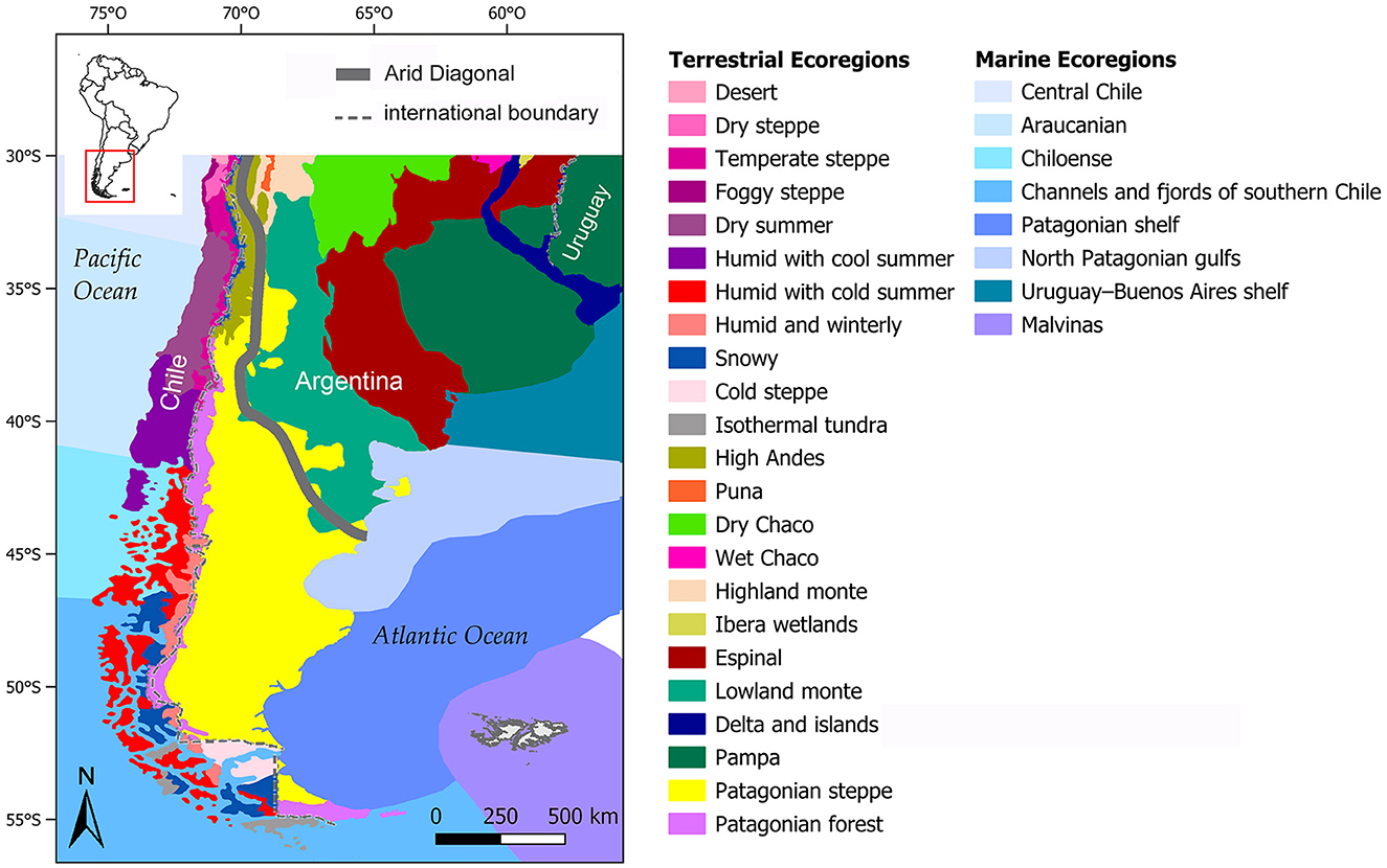
Figure 1. Distribution of terrestrial and marine ecoregions in southern South America (Argentina and Chile, 30°-56° S). Modified from Gedeco Ltda (2008), Morello et al. (2012), and Spalding et al. (2007).

The South American landmass has the approximate shape of an inverted isosceles triangle that narrows toward the south, especially from the Tropic of Capricorn (Pineau et al., 2003), giving the southern tip of South America the character of a peninsula that penetrates deeply into the Pacific and Atlantic oceans (Morello, 1984). This particular geometry propitiates the existence of certain N-S gradients, such as those of increasing morphostructural and ecosystemic simplicity (e.g., lower biodiversity in terrestrial ecosystems) and of increasing maritime influence (i.e., oceanicity; Fairbridge and Oliver, 1987), the latter resulting in less rigorous and more homogeneous environments than would be expected based on latitude alone (Morello, 1984; Pineau et al., 2003).

Throughout the area considered in this study, rainfall is distributed very heterogeneously on both sides of the Andes, with arid or semi-arid environments predominating on the eastern slope (Morello, 1984). The most conspicuous feature there is the South American Arid Diagonal (de Martonne, 1935), which crosses the area in a NW-SE direction. This extensive strip, with a marked latitudinal development and variable width, forms a series of successive arid enclaves that interrupt the continuity of the humid zones, according to a combination of factors that are staggered from north to south over the different circulation zones (Bruniard, 1982).

In the northwest, the Subandine and Pampean Sierras divide the arid strip into plateaus, basins and valleys, under a double leeward effect caused by the orographic interruption of the already weakened influences of both the Atlantic and the more sporadic influences of the Pacific. Further south, in full domain of the westerlies, the Patagonian aridity extends to the Atlantic coast (Bruniard, 1982). During the Quaternary, the central position of the Arid Diagonal remained more or less constant (Abraham et al., 2000; Garleff and Stingl, 1998), although with minor variations throughout the Holocene due to climatic oscillations (Mancini et al., 2005).

The effect of the Arid Diagonal on the biota was and is significant. The sclerophyllous forest and the scrubland located in central Chile (with a Mediterranean subtropical climate) and the temperate forest located immediately south of the former, integrate one of the core biomes that became progressively isolated from the other humid South American formations, the closest being the Yungas forest in northwestern Argentina, the humid Pampas and the Chaco-type forests of the Espinal. Between these more humid areas, the desert or semi-desert floristic formations along the Arid Diagonal developed (in our study area, the Monte and Patagonian steppe deserts) (Cabrera and Willink, 1973).

In addition to the varied terrestrial ecosystems, there are marine ecosystems corresponding to the Argentine Sea, which encompass the portion of the continental margin of the southwestern Atlantic exposed to the ecological effects of the fronts generated by the Brazil and Malvinas currents (Falabella et al., 2009; Zárate, 2013). These bodies of water coexist and mix, which determines important physical-chemical gradients and the presence of high concentrations of nutrients (Zárate, 2013). The rich primary productivity of these waters is the basis of a complex trophic web that culminates in superior predators of different taxonomic groups, which play a key role as regulators of lower levels (Falabella et al., 2009; Zárate, 2013).

The climate in southern South America during the late Holocene (i.e., the last 4,000 years BP) was characterized by fluctuating conditions in terms of temperature and humidity, within a general cooling trend from the late mid-Holocene onwards (Berman et al., 2020; Silvestri et al., 2021, 2022). Such fluctuations in climatic conditions are linked to intervals such as the Medieval Climate Anomaly (MCA) and the Little Ice Age (LIA) (Lüning et al., 2019; Silvestri et al., 2021), which caused shifts in the distribution of plant and animal lineages (Tonni, 2006). Despite these oscillations, the overall spatial distribution of biomes in the study area appears to have changed relatively little (i.e., temporal changes in biomes consisted mainly of variations in the position of their respective boundaries; see maps in Maksic et al., 2018). Regarding the relative C₃/C₄ composition of ecosystems, in Central Argentina there is evidence of a continuous replacement of C₄ plants by C₃ plants since the beginning of the late Holocene. During this period, the relative abundance of C₃ plants in grasslands, shrublands, and forests increased by an average of 32% (Silva et al., 2011). This partial and progressive replacement coincided with climate changes toward cooler and wetter conditions compared to those prevailing in the mid-Holocene (Silva et al., 2011), which had consequences for the current spatial distribution of δ¹³C (‰) and δ¹⁵N (‰) values of terrestrial primary production (Figure 2).

Figure 2

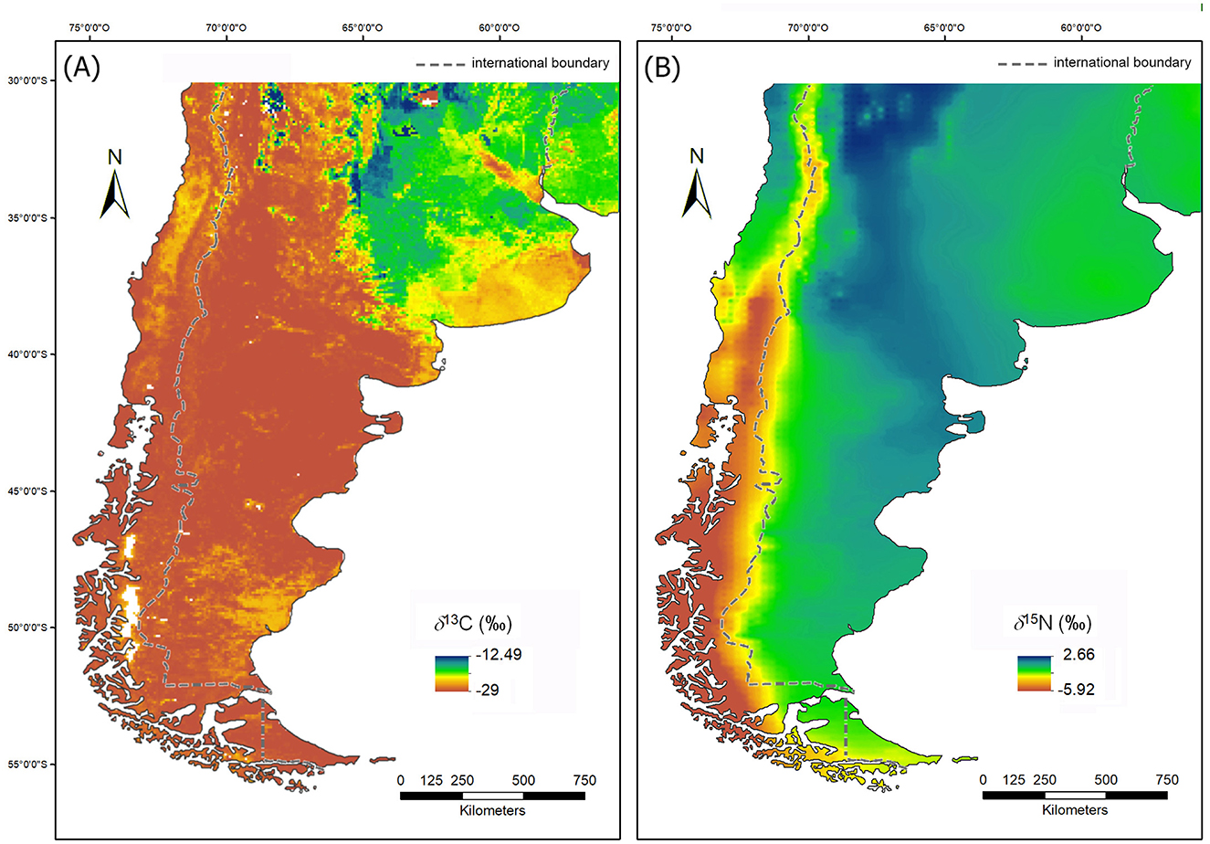
Figure 2. Plant δ¹³C and δ¹⁵N isoscapes. (A) Values of δ¹³C estimated based on the C₃/C₄ composition (Powell et al., 2012); (B) values of δ¹⁵N predicted as a function of mean annual temperature and mean annual precipitation based on the regression model of Amundson et al. (2003) (after Bowen and West, 2008). Both maps were processed from the original files provided by the cited authors.

3.2 Human subsistence in the late Holocene

Most late Holocene human populations in this vast portion of southern South America relied primarily on terrestrial resources for their subsistence, within a fairly widespread hunting, gathering, and fishing economy (Borrero, 1994–1995, 2001; Politis, 2008; Politis and Borrero, 2024; Scheinsohn, 2003). The only exception were the canoe-based hunters who inhabited the fjords and islands of southern Chile, whose ethnographically known representatives (Yámana, Kawésqar, and Chono) exhibited authentic maritime adaptation (sensu Erlandson and Fitzpatrick, 2006), whose origins date back 6,000 years BP, according to archaeological evidence (McEwan et al., 1997; Reyes et al., 2019). However, even in these populations, consumption of terrestrial resources such as fungi, berries, and mammals (e.g., rodents, huemul, guanaco) is documented (Gusinde, [1937] 1986; McEwan et al., 1997; Orquera and Piana, 1999; Reyes et al., 2019). Along the Atlantic coast, particularly in Patagonia, archaeological evidence indicates the recurrent exploitation of marine biota (e.g., Castro et al., 2004; Gómez Otero, 2007; Zangrando and Tivoli, 2015). In this case, however, this occurred without the development of navigation technology or intensive exploitation of resources beyond the tidal zone, configuring what Beaton (1991) called coastal use.

The northwestern portion of the study area, on both sides of the Andes, lies within the dispersal zone of maize, the introduction of which dates back to 3,000–2,500 years BP. However, on the eastern slope of the Andes, the economic importance of this resource seems to have been more recent (ca. 1,500–1,000 years BP), when an agricultural economy was established in at least some areas of the region (Gil et al., 2014, 2018; López et al., 2020; Neme, 2007; Pastor and López, 2010; Pastor and Gil, 2014). A truly stable agricultural economy seems to have been present also in central Chile from approximately 2,000 years BP (Alfonso-Durruty et al., 2023; Falabella et al., 2008). In the northeastern part of the area, around the Paraná and Uruguay river systems (del Plata Basin), an increase in the production and consumption of maize, as well as other cultigens, is inferred from ca. 2,000–1,000 years BP, associated with the dispersal of a horticultural economy (Loponte and Acosta, 2013; Politis and Bonomo, 2012). Finally, in the last centuries of the pre-Hispanic period, there seems to have been manipulation and culinary processing of maize by groups of hunter-gatherers from the Pampas and northern Patagonia regions (Lema et al., 2012; Musaubach and Berón, 2012; Prates et al., 2019; Saghessi, 2024). In this case, there is no evidence of local production due to climatic limitations, so it is inferred that the presence of maize is a product of exchange or trade with societies established in other regions (López et al., 2020; Musaubach and Berón, 2012; Prates et al., 2019; Saghessi, 2024).

In summary, it can be said that, beyond local or regional variations in subsistence, Late Holocene human populations in Argentina south of the 30° S parallel generally fall within the “foragers” category, as defined by Porter and Marlowe (2007): < 10% agriculture, < 10% animal husbandry, trade accounting for < 50%, and no more than any single local source. Other subsistence economies (horticulture, agriculture) appear to have been highly restricted both in space and time (i.e., the last 2,000 years BP).

4 Materials and methods

This section, in which we will detail all the materials and the methods used in our study, is made up of four subsections, namely: Rationale for the approach, Description of the dataset, Primary processing of data (Supplementary Data Sheet 2), and Secondary processing of data. To the extent that the results of the primary processing of the data inform the decisions involved in its secondary processing, those results will be described immediately after the description of the corresponding method (Supplementary Data Sheet 2). The results of the secondary processing of the data, related to the very purpose of this paper, will be described in Section 5.

4.1 Rationale for the approach

A detailed account of the rationale for our approach can be found in Barrientos et al. (2020). Here we will only outline its main features.

(a) Our methodology is geographically explicit in the sense that uses geographic data to model and analyze, in a GIS environment, how organism variables (e.g., stable isotope values and TP) and biotic and abiotic environmental variables (e.g., latitude, effective temperature, productivity, biodiversity) relate to each other.

(b) Maps of isotopic variables—generically called isoscapes (i.e., cartographic models about geographically patterned variation in isotopic compositions of a substrate; Bowen, 2010; Bowen et al., 2009; West et al., 2010)—and of derived variables like TP, are resources that have a redescriptive, comparative, and heuristic value. They are redescriptive devices in the sense of providing a new and more complete description of the phenomenon of isotopic variation by explicitly adding the spatial dimension, which is missing in most studies of stable isotopes. Isotopic maps for a given taxon allow simultaneous comparisons between multiple ecosystems, provided that an appropriate baseline is established. At the same time, they allow comparisons or operations to be made with other maps, such as those representing δ¹³C (‰) and/or δ¹⁵N (‰) values of terrestrial primary production (e.g., Bowen and West, 2008; Powell and Still, 2009; Powell et al., 2012) or of primary consumers (e.g., Barrientos et al., 2020). Finally, they are heuristic in the sense of allowing the discovery of new facts (e.g., patterns and/or relationships) that are difficult to perceive by other means.

(c) Our approach explicitly privilege space over time. This does not imply ignoring the importance of time as the axis along which systems evolve, but rather recognizing the difficulty of its treatment when working on large spatial scales and with big datasets with a relatively low temporal resolution. In large-scale studies, it is practically impossible to have a convenient amount of synchronous or near-synchronous data, so maximum spatial coverage is achieved by including cases corresponding to specific time blocks. Under such conditions what is generated are time-averaged constructs akin to what Vander Zanden et al. (2014) have called “long-term isoscapes.” Nevertheless, this should not be seen as a disadvantage, but rather as an opportunity to identify and study cumulative patterns revealing strong relationships between persistent trophic interactions and places. What is lost in terms of ecological realism is gained in terms of visualization and understanding.

4.2 Description of the dataset

We compiled a dataset consisting of a total of 1,148 georeferenced individual cases, of which 1,146 correspond to δ¹³C (‰) values and 1,018 to δ¹⁵N (‰) values. These data were obtained by bulk stable isotope analysis (BSIA) of bone and dental collagen extracts from human burials assignable, either by direct radiocarbon dating or by context, to the late Holocene (i.e., from 4.2 ka BP to historical times before the 20^th century). However, the vast majority of cases (76%) correspond to the last 1,500 years BP (considering the midpoint of the calibrated age range) (Figure 3). These data come from human remains recovered from archaeological sites in Chile, Argentina, Uruguay, and Brazil, located south of 30° S and between 52° and 75° W. Most of the data were taken from the South American Archaeological Isotopic Database (SAAID) (Pezo-Lanfranco et al., 2024), with other data not included in that database being added. In cases where mistakes or inaccuracies were detected in the SAAID, these were amended (Supplementary Table 1).

Figure 3

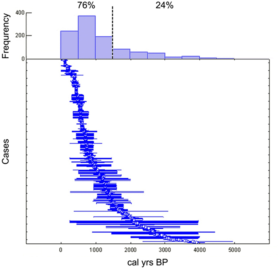
Figure 3. Range plot with histogram depicting the distribution of calibrated age ranges (obtained from direct or contextual dating) of the cases included in this study. Blue lines show the ranges; white circles mark the mid-points.

The isotopic data correspond to adult individuals or weaned subadults. The attribution of the weaned character was made, in each case, based on published information about the individual's age at death or the age of the sampled tissue (in the case of dental collagen) or was inferred from the comparison with isotopic values of adult individuals from the same region. Since information on the quality of the collagen extracts is lacking in a large percentage of cases (40.2%), stable isotope ratios were taken at their face value. Otherwise, a large-scale spatial study such as the one described here would be virtually impossible due to the small sample size. Only cases reported as erroneous or doubtful by the authors of the original publications or those with an atomic C/N ratio >3.6 indicative of contamination with humic substances (Guiry and Szpak, 2021) were excluded. For the sites in Argentina, where most of the analyses are focused, information on altitude (in meters above sea level or masl) and distance to the Atlantic Ocean (in km) was obtained. In both cases, this was done in a GIS platform (ArcGis 10.8.2; ESRI 2021) using the measurement tools provided by the software package. Altitudinal data were extracted from a digital elevation model or DEM (Global 30 Arc-Second Elevation, Sheets W100S10 and W60S10; United States Geological Survey, 2016) and distances to the sea were measured, in most of the study area, using a vector layer of the Atlantic coast. However, between 30° and approximately 37° S, the distance was calculated to the Uruguay and de la Plata rivers, two important watercourses in the distal part of the del Plata Basin along which the international border between Uruguay and Argentina runs, using a hydrographic vector layer.

4.3 Secondary processing of data

4.3.1 Mapping of transformed isotopic niches

The maps we will present in this paper are intended to constitute a first approximation to the problem of the spatial distribution of transformed isotopic niches in southern South America. Therefore, the procedure for their construction were kept as simple as possible, even at the risk of making simplifying methodological decisions, as will be discussed in each of the following sections.

4.3.1.1 Interpolator selection

For the mapping of transformed isotopic niches and of their precursor inputs (i.e., distribution of δ¹³C [‰] and δ¹⁵N [‰] values of human samples and δ¹⁵N [‰] values of primary producers) we decided to use the inverse distance-weighted (IDW) interpolation method (Shepard, 1968) due to its flexibility and ease of use (Hengl, 2007). This method assumes that each measured point has a local influence on unsampled locations moderated by the distance decay effect (Wang et al., 2019). It is not exact as it does not generate an estimate that is equal to the observed value at a sampled point (Li and Heap, 2008; Myers, 1994); however, it can be forced to be exact (Burrough and McDonnell, 1998). More importantly, this interpolator is not based on any theory or assumption, being strictly heuristic. Precisely, one of its main advantages is that it is not necessary to fit the data to a model, as occurs with geostatistical methods such as kriging, since it is not restricted by the covariance and variance functions (Wang et al., 2019). It could be used on very small data sets, allowing interpolation from data scattered on a regular grid or irregularly spaced samples (Burrough and McDonnell, 1998; Shepard, 1968). As a disadvantage, it does not provide any measure of the reliability of the interpolated values. In this sense, it is deterministic in that it does not incorporate associated errors and only produces the estimates (Hengl, 2007; Li and Heap, 2008). While IDW lacks a built-in function to deal with errors associated with the estimate, these can nevertheless be calculated separately and then mapped. This is the case of the difference between predicted values and input or measured values (i.e., interpolation error) or the results of cross-validation. The latter is a procedure for testing the quality of a predicted data distribution by removing one data location and then predicting the associated data using the data at the rest of the locations. In cross-validation performed in ArcGis, the comparison between the predicted value and the input or observed value is expressed in statistics such as the mean error or the root mean square error.

The traditional IDW interpolator, despite its flexibility, ease of use, and model-free character (main reasons that justified its use in this exploratory spatial modeling approach of isotopic niches), is not a really good method to deal with clustered data like ours. More appropriate and powerful alternatives to deal with this problem in the spatial structure of the data are kriging (Pyrcz and Deutsch, 2002, 2014) and the recently developed dual IDW (DIDW) (Li, 2021; Li et al., 2019). Regarding the former, a previous experience of the authors with ordinary kriging (Catella et al., 2018) shows that this interpolator does not necessarily perform better in relation to our objectives and, regarding the latter, it is certainly an option to consider in future studies, especially when it becomes incorporated into GIS packages. Beyond all these considerations, it should not be lost sight of that, in an exploratory study such as the one described here, the level of tolerance to error due to the interpolator and the setting of its parameters could be higher than when economic or management decisions are involved.

The IDW interpolation was performed in ArcGis 10.8.2 with a power parameter (p) equal to two, using between 12 and 40 neighbors within a circular window of 500 km radius with four sectors. Within each sector, between three and ten points were sampled to define an even neighborhood in all directions. All raster coverages were generated with a cell size of 4,000 meters per side. When there was more than one δ¹⁵N (‰) value for the same site or location, all data were considered. To assess the strength of the association between the δ¹³C (‰) and δ¹⁵N (‰) values measured in bone and those resulting from interpolation, the Spearman rank correlation coefficient (r_s) was calculated and, to verify the absence of significant statistical differences between paired observations, the Wilcoxon matched pairs test was performed. In both cases, the alpha level was set at 0.01. For each isotopic system, error calculated by cross-validation was mapped using IDW with p = 3, in order to highlight the areas of greatest variation between interpolated and input data. The error tolerance boundary was set at ±1 ‰. The mean error and the root mean square error were also calculated.

In all maps, the area represented is smaller than the total interpolated area, since the cases from eastern Uruguay and southeastern Brazil—and, to some extent, also those from Chile and western Uruguay, that are shown but will not be discussed beyond some occasional reference—were included only to avoid the edge effect (Conolly and Lake, 2006).

4.3.1.2 δ¹⁵N (‰) baseline selection

When the purpose is to integrate isotopic information from diverse geographic locations into a single study, it is essential to have a common comparison standard allowing such integration. In the case of δ¹⁵N (‰) this is because substantial variation is expected, even between spatially close environments, in the isotopic ratios at the base of the food web from which all consumers ultimately extract the nitrogen they assimilate (Post, 2002). A δ¹⁵N (‰) baseline is not only useful for calculating TP within a single ecosystem (e.g., Hansson et al., 1997; Keough et al., 1996; Peterson et al., 1985), but also for monitoring variation in δ¹⁵N (‰) among different ecosystems. In the absence of adequate estimates of the baseline δ¹⁵N (‰) in each system, it is virtually impossible to determine whether spatial dissimilarity in δ¹⁵N (‰) values among individuals of a geographically and ecologically wide-ranging species is due to regional variation in food web structure or to regional differences in the isotopic baseline (Cabana and Rasmussen, 1996, p. 10844; Post, 2002, p. 704). Therefore, one of the most critical aspects of using bulk bone collagen δ¹⁵N (‰) to estimate TP of current or past individuals, populations, or species is to obtain the isotopic baseline that allows comparisons across multiple systems (Anderson and Cabana, 2007; Cabana and Rasmussen, 1996; Casey and Post, 2011; Post, 2002).³

In this and a previous paper (Barrientos et al., 2020), we argue for the need to have, in a study of the nature of the one presented here, a single raster layer representing the baseline for δ¹⁵N (‰). This is more feasible to do so using data from terrestrial primary production than from a primary consumer, contrary to what is usually recommended for studies carried out at a smaller spatial scale and in aquatic environments (Anderson and Cabana, 2007; Cabana and Rasmussen, 1996; Vander Zanden and Rasmussen, 2001). For this reason we will use, for constructing our δ¹⁵N (‰) baseline, data derived from a global-scale regression model based on the integration of empirical observations of modern plant δ¹⁵N (‰) values and environmental data (continuous MAT and MAP fields for the normal climatic period 1961–1990) (Bowen and West, 2008; based on Amundson et al., 2003). The model output, further masked using continuous vegetation fields, eliminating areas with >80% non-vegetated ground (Bowen and West, 2008), was kindly provided in Erdas Imagine (.img) format by Drs. G. J. Bowen and J. B. West. The two main disadvantages of using an actualistic global model such as this are that: (a) it extrapolates into the past a distribution of isotopic values that may not correspond, in all its details, to that existing during the period in question and (b) there is a fairly large uncertainty associated with the predictions of the model equation, so that the differences between the predicted and observed δ¹⁵N (‰) values can be very large in some locations (Bowen, 2010; Pardo and Nadelhoffer, 2010). However, these disadvantages are compensated by its ease of implementation and the fact that it provides an objective and unique basis for performing TP calculations over a very large surface. As we already expressed in Section 4.1, in this exploratory study we privilege, within certain limits, visualization and understanding over ecological realism. To optimize, the original raster layer was cropped to fit the size of the study area and then, to improve resolution, an additional interpolation was performed using as input the δ¹⁵N (‰) value corresponding to each of the cells (IDW; p = 2).

4.3.1.3 Selection of trophic enrichment factor

The δ¹⁵N (‰) increases in a predictable way between a consumer and its diet (Anderson and Cabana, 2007; Caut et al., 2009; DeNiro and Epstein, 1981; Post, 2002; Vander Zanden and Rasmussen, 2001). Differences in δ¹⁵N (‰) between a consumer and its diet are referred to as the trophic enrichment factor or TEF (also expressed as Δ¹⁵N_{diet − body}). The amount of the increase in δ¹⁵N (‰) values represented by the TEF, which is due to the isotope discrimination process whereby the heavier isotope ¹⁵N increases in abundance compared to the lighter isotope ¹⁴N, has been and continues to be much debated (see reviews in Bocherens and Drucker, 2003; Caut et al., 2009; Hedges and Reynard, 2007; Lewis and Sealy, 2018; O'Connell et al., 2012). The TEF varies between tissues within individual consumers due to metabolic fractionation (DeNiro and Epstein, 1981; Hobson and Clark, 1992; for humans see Kraft et al., 2008; Nash et al., 2009; O'Connell and Hedges, 1999; O'Connell et al., 2001; Richards, 2006; Schoeller et al., 1986). In the case of bone collagen, the most frequently sampled biomolecule in paleodietary studies, O'Connell et al. (2012) have estimated a range of +5.9 ‰–+6.3 ‰ for the Δ¹⁵N_{diet − collagen} offset. Some authors propose using ranges (e.g., +3 ‰–+5 ‰; Bocherens and Drucker, 2003) or different values within those ranges (e.g., +3 ‰ or +6 ‰; Lewis and Sealy, 2018) rather than a single value, as is the common practice. In addition to the uncertainty surrounding the estimation of TEF between consumer tissues and those of their sources, this trophic level effect also appears to vary considerably across a range of environmental (e.g., temperature, altitude, aridity) and physiological (e.g., water stress, starvation) conditions, as well as diet composition (McCue and Pollock, 2008; McCutchan et al., 2003; Vanderklift and Ponsard, 2003). In this paper we used a TEF of +5 ‰ between diet and collagen of humana consumers since this produced the best fit between the δ¹⁵N (‰) isoscape of plants (Bowen and West, 2008) and that of a primary consumer, the guanaco (Lama guanicoe), a camelid that was exploited as a staple food by many human populations in the study area throughout the late Holocene (Barrientos et al., 2020). A TEF of +5 ‰ between diet and collagen of human consumers is within the Δ¹⁵N_{diet − humancollagen} offset experimentally derived by O'Connell et al. (2012) (+4.6–6.3 ‰), considering both conservative and less-conservative estimates.

4.3.1.4 Calculation of trophic position

To achieve this goal, we followed the general guidelines described in Barrientos et al. (2020). These are useful to calculate, in a GIS environment, the interpolated map of TP for a given species from two layers of information: the δ¹⁵N (‰) isoscape of the isotopic baseline (δ¹⁵N_baseline [‰]; in our case study, the modern primary producers or MPP) and b) the δ¹⁵N (‰) isoscape of the species in question (in our case, the archaeological humans or AH). To calculate the TP_{archaeologicalhumans}, it is necessary to implement the following formula (adapted from Anderson and Cabana, 2007) in the raster calculator tool of the GIS platform to perform the corresponding operations between layers:

$\begin{array}{l}T{P}_{\text{archaeological humans}}=([AHI-MPPI]/5)+1,\end{array}$

where AHI is the δ¹⁵N (‰) isoscape of archaeological humans, MPPI is the δ¹⁵N (‰) isoscape of the modern primary producers, 5 is the selected TEF (+5‰), and 1 is the trophic level corresponding to the δ¹⁵N_baseline (‰) (i.e., MPP).

From the TP raster layer, the data corresponding to the individual cases were extracted and the non-parametric correlation coefficient r_s (alpha = 0.01) was calculated between these and the input and interpolated δ¹⁵N (‰) values.

4.3.1.5 Mapping of transformed isotopic niches

As stated in the Introduction, an isotopic niche can be defined as the point or area occupied by an individual or a set of individuals within a δ space (Bearhop et al., 2004; Jackson et al., 2011; Layman et al., 2012; Newsome et al., 2007, 2012). In this paper we define the transformed isotopic niche as the cell value in a raster layer resulting from combining two other layers: (a) that representing the spatial variation in the TP calculated for a given taxon (derived from δ¹⁵N [‰] values) and (b) that representing the spatial variation in δ¹³C (‰) for such taxon. The set of all cells with the same value will constitute the geographic expression of the niche, which may be spatially continuous or discontinuous.

In order to build the map of transformed isotopic niches we proceeded, first, to reclassify the layer called TP_{archaeologicalhumans} into five intervals, assigning each of them a code from 1 to 5, where 1 indicates the lowest TP (< 2.5) and 5 represents the highest TP (>4). A similar procedure was performed with the δ¹³C (‰) layer. In this case the reclassification included two intervals limited by the value −16 ‰ (< -16 ‰ ≤ ). This value approximately corresponds to the point above which the contribution to the diet of C₄ plants and marine food is estimated to be more than 50% (from data published by Pate and Schoeninger, 1993). δ¹³C (‰) values < -16 ‰ were assigned code 10, and values equal or greater than that value were assigned code 20. Then, using the ArcGis 10.8.2 raster calculator, both raster layers were added, resulting in the transformed isotopic niche model, where values from 11 to 15 indicate niches with δ¹³C (‰) values < -16 ‰ and increasing TP, while values from 21 to 25 indicate niches with δ¹³C (‰) values equal or >-16 ‰ and increasing TP.

4.3.2 Assessment of spatial variation in human omnivory

Degrees of human omnivory were measured in terms of the TP, calculated on the basis described in Section 2.3.1.4. To facilitate discussion, the different degrees of omnivory were grouped into three broad omnivory categories (OC): I (2 ≤ TP < 3), II (3 ≤ TP < 4), III (TP ≥ 4). OC I corresponds to a typical omnivorous diet, incorporating variable proportions of plant foods (primary producers) and animal foods (mainly primary consumers). OC II corresponds to an omnivorous diet incorporating a higher proportion of foods of animal origin (mainly but not exclusively, primary consumers). OC III corresponds to an omnivorous diet mainly consisting of animal foods (primary and secondary consumers, the latter mostly marine). OC II and III reflect an increasing importance of the predatory component of subsistence (i.e., hunting and fishing) over the gatherer component.

It is worth mentioning, however, that the presence of marine protein in the diet will naturally tend to bias the results toward OC II and III, even if the total amount of animal protein is relatively small. This is particularly critical in the case of the transition from OC I to II, which is particularly sensitive to subtle changes in the proportion of marine protein vs. terrestrial protein, even if the total amount of protein remains unchanged. In contrast, a considerable amount of marine protein is required for an individual to move to the OC III category, making the transition from OC II to III less problematic from an interpretive perspective. In this initial contribution we will not delve into the implications of this caveat, but it should be noted that a fine-tuning adjustment based on a mass balance model would be required to analyze those critical points where small changes in the proportion and δ¹⁵N (‰) value of marine protein can change the OC assigned to an individual.

5 Results

5.1 δ¹³C (‰) and δ¹⁵N (‰) human isoscapes

As we have already demonstrated in Supplementary Data Sheet 2, one of the environmental variables that influence the spatial variation of isotopic values, particularly δ¹⁵N (‰), is latitude (Supplementary Data Sheet 2, Supplementary Figure 2D). Figure 4 shows the results of the interpolation of δ¹³C (‰) and δ¹⁵N (‰) values of human bone and tooth samples from southern South America. Although the maps were generated with information covering the entire late Holocene period, the temporal structure of the data—as mentioned in Section 4.2—means that the overall picture is strongly influenced by cases younger than 1,500 years BP, which constitute 76% of the total.

Figure 4

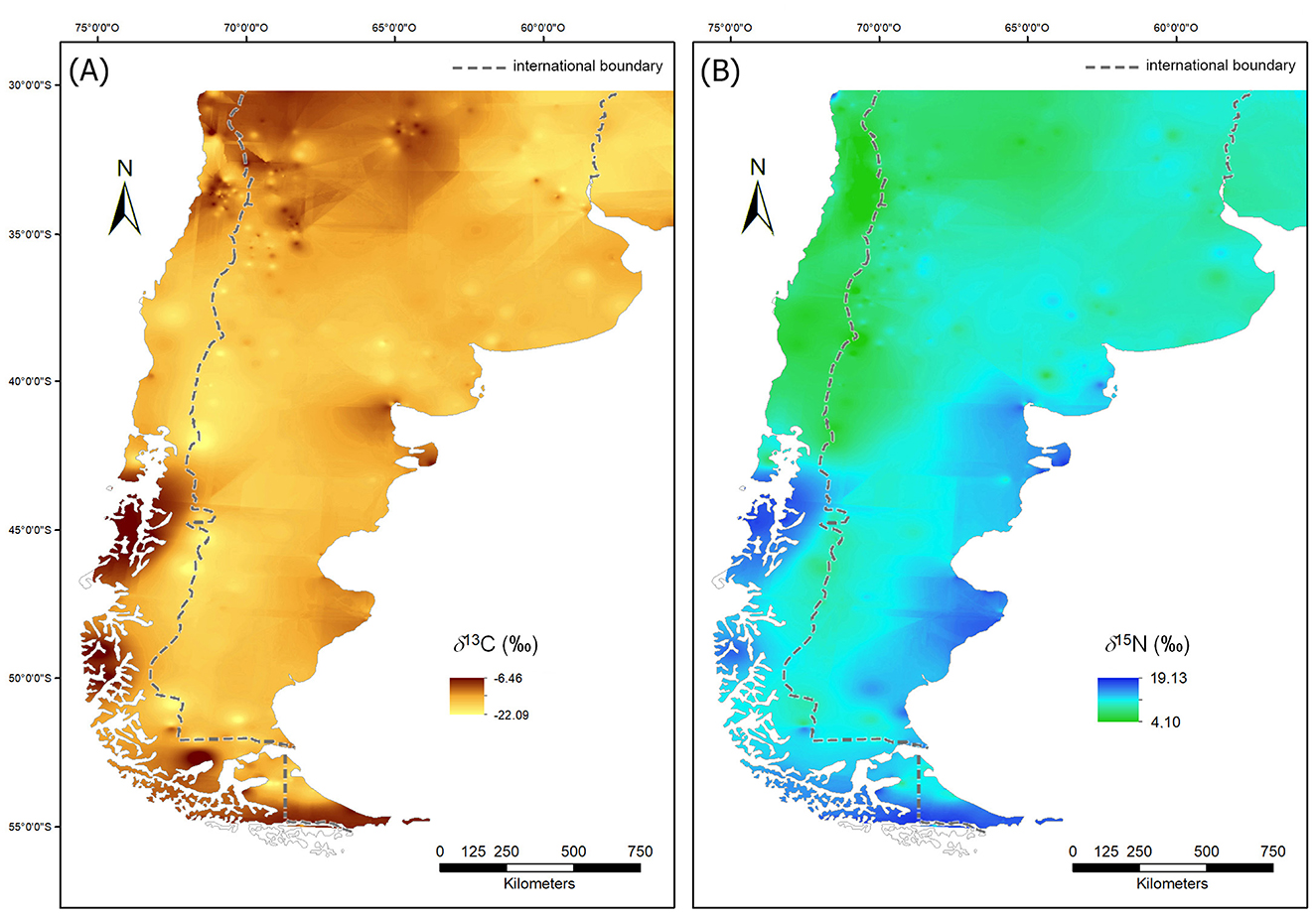
Figure 4. Archaeological human isoscapes (IDW interpolation): (A) δ¹³C; (B) δ¹⁵N.

Regarding the quality of the generated maps, the results of the non-parametric correlation analysis performed between the input and interpolated δ¹³C (‰) and δ¹⁵N (‰) values indicate the existence of a high and significant correlation between these two variables (δ¹³C: r_s = 0.9; p < 0.01; δ¹⁵N: r_s = 0.95; p < 0.01), while the results of the Wilcoxon matched pairs test show the absence of significant differences between these same variables (δ¹³C: T = 294,124; Z = 0.46; p > 0.05; δ¹⁵N: T = 242,115; Z = 0.13; p > 0.05).

Figure 5 display the spatial distribution of the results from cross-validation analysis. In general terms, it can be said that the errors in the estimation of the δ¹³C (‰) and δ¹⁵N (‰) values from the input data are relatively low and spatially circumscribed, mostly restricted to those sectors where the spatial autocorrelation of the variable in question is lower (i.e., where there is greater variation in the values of the variable between relatively close places). However, it is observed that the magnitude of the error is greater in the δ¹³C (‰) (mean error = 0.04; root mean square error = 1.81) than in the δ¹⁵N (‰) (mean error = 0.03; root mean square error = 1.7).

Figure 5

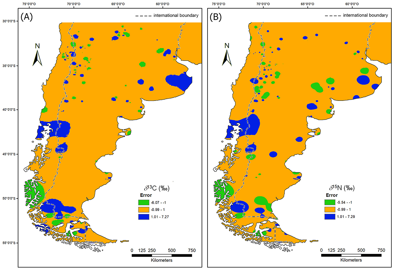
Figure 5. Maps of the cross validation error: (A) δ¹³C; (B) δ¹⁵N. In orange areas where the error is ±1 ‰, in green areas with an error lower than −1 ‰ and in blue areas with an error higher than 1 ‰.

5.2 Transformed isoscape

As for TP (Figure 6), north of the parallel of 35° S (first latitudinal band or LB1) predominate values lower than 3, which indicates the existence of diets based on the consumption of a high proportion of either wild or domesticated plant resources. At the northwestern corner of the area, on both sides of the Andean Mountains, there are two spatial nuclei with TP values close to those of primary consumers (i.e., ≈2). Between 35° and 40° S (second latitudinal band or LB2), TPs between 2.5 and 3.0 and between 3.0 and 3.5 occupy approximately equal areas, the former mainly west of 65° W and the latter east of that meridian. Between 40° and 45° S (third latitudinal band or LB3) TPs between 3.0 and 3.5 predominate, with a small area in the NW with TPs between 2.5 and 3.0, representing the southernmost expression of a continuous area strongly influenced by the consumption of plant resources. In this latitudinal band, TPs higher than 3.5 appear, both on the Atlantic and Pacific coasts, indicating the existence of diets that incorporate varying degrees of marine resources. Between 45° and 50° S (fourth latitudinal band or LB4), TPs below 3 are represented only by a small area located near the Andes, surrounded by a wide central area with TPs between 3.0 and 3.5. In this latitudinal band, TP values > 3.5 are widely expressed in coastal areas of the two oceans. Finally, between 50° and 55° S (fifth latitudinal band or LB5), TPs > 3.5 are the majority, with a broad representation in continental and island coastal areas of TPs > 4.

Figure 6

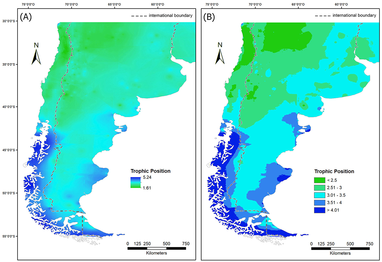
Figure 6. Maps of the human trophic position (TP) (transformed isoscapes): (A) continuous map; (B) map classified in intervals of 0.5.

5.3 Transformed isotopic niches

Regarding transformed isotopic niches (Figure 7), the one with the greatest geographical extension, crossing the five latitudinal bands diagonally with a NE-SW orientation, is that characterized by TP values between 3 and 3.5 and δ¹³C (‰) values lower than −16‰. Within the δ space and the one where TP replaces δ¹⁵N (‰), this niche occupies the position of highest kernel density (Supplementary Figures 3B, 6B). In the northwestern sector of the map, occ mountain range, and up to just south of 40° S, there is a niche characterized by a high consumption of terrestrial plants. North of 35° S, a greater predominance of C₄ plants is observed, and south of this parallel, with a greater consumption of C₃ plants. South of the 40° S, a high representation of niches with a strong marine component is observed. On the Pacific coast, this niche shows a continuous distribution, while on the Atlantic coast, it is limited to the main peninsulas of Patagonia.

Figure 7

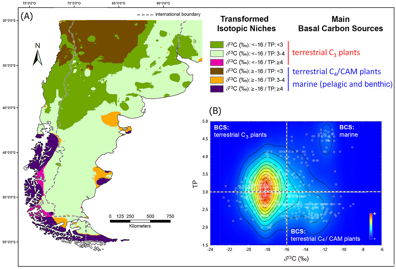
Figure 7. (A) Map of the human transformed isotopic niche; (B) kernel density map of human samples where the transformed δ space is subdivided condidering thresholds values for main basal carbon sources (BCS).

5.4 Omnivory categories

Figure 8 represents the geographic distribution of three categories of omnivory (Figure 8A) and its median distribution along the five longitudinal bands analyzed in the territory of the Argentine Republic (Figure 8B). Regarding laititudinal bands, in LB1 the largest area is found in OC I—characterized by a high dependence on the vegetal component of the diet—which is continuously located toward the west and alternates with OC II—with a greater component of terrestrial herbivores and a lower and variable dependence on vegetal resources and/or aquatic resources—toward the east. LB2 shows an approximately equal distribution of OC I and II, where OC I is found over the western half and OC II over the eastern half. LB3 shows a wide representation of OC II in the mediterranean area. This is the southernmost band where OC I is represented and the northernmost one where OC III occurs. Both are present in small áreas, the first one over the mountain range (to the west), and the second on both coasts (Atlantic and Pacific). In LB4, approximately equivalent areas of OC II are found, toward the interior, and OC III on the coast. Finally, in LB5, most of the surface is covered by OC III, while OC II is restricted to a small sector in the interior.

Figure 8

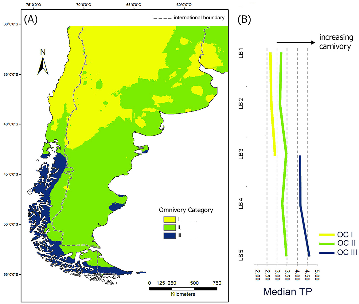
Figure 8. (A) Map of human omnivory categories (OC); (B) median variation of Trophic Position (TP) in each OC across latitudinal bands (LB1 to LB5), sectors with no lines are those where the OC is absent.

6 Discussion

In the study area, spatial variation in human omnivory during the late Holocene was markedly structured (Figure 8). The spatial arrangement of the OCs, which follows a general diagonal pattern, indicates an increase in carnivory in a NW-SE direction. In OC I, both plant and animal foods corresponded to organisms integrated into food webs fueled by different BCSs (mainly C₄/CAMS plants in the NW corner and C₃ plants in the rest of the distribution area) (Figure 7). In OC II, the plant and animal foods consumed also came from food webs with BCSs corresponding to C₃ and C₄/CAMS plants, mainly north of the parallel of 42° S and C₃ plants and marine BCSs (pelagic and/or benthic) south of that parallel. In OC III, expressed only in particular coastal zones of Patagonia, the foods consumed—mostly of animal origin—came from terrestrial and marine food webs, in the first case with BCSs corresponding to C₃ and CAMS plants (e.g., Kochi et al., 2024) and, in the second case, with marine BCSs (pelagic and/or bentic) (e.g., Kochi et al., 2018).

It is worth asking what factors likely influence the observed spatial structure in terms of transformed isotopic niches and, above all, in terms of omnivory categories. Below we will deal with those that we consider to be the main ones, namely net primary productivity (NPP), effective temperature (ET) ranges, and differential distribution of marine biota. The explanatory value of other factors that purportedly increase the degree of carnivory, such as the environmental scarcity of Na and N (see Section 2), will not be addressed here due to the current lack of relevant information on the differential soil concentration of these elements in most of the study area.

6.1 Net primary productivity

Net primary productivity (NPP) is the amount of fixed energy or organic matter remaining after plants have met their own respiratory needs. It is equivalent to the amount of energy available to consumers, including humans (Knapp et al., 2014). This variable is strongly and inversely correlated with latitude (Stelling-Wood et al., 2021). This pattern is associated with higher mean annual temperatures, longer growing seasons, and increased precipitation at lower latitudes compared to higher ones (Stelling-Wood et al., 2021).

In our study area, there is a weak positive correlation between NPP⁴ and TP (r_s = 0.34; p < 0.001). The greatest dispersion of TP values occurs in areas with medium NPP values (Figure 9A). Figure 9B shows the overlap of the zones with different NPP (classified into three grades: < 0.4, 0.4–0.6, and >0.6 kg-C/m²/year, which correspond to low, medium and high values, respectively) and the zones corresponding to each omnivory category. It can be seen that OC I tends to occur in areas of low and medium NPP (58.3% and 24%, respectively). This suggests a close association between diets with a high plant component (i.e., low carnivory, whether due to a foraging or agricultural subsistence economy) and low- and medium-productivity terrestrial environments, located in the northwest and central west of the study area. An exception would be the zones that present a low degree of carnivory in areas of high terrestrial productivity (17.1%). These are located in the lower part of del Plata basin and in smaller and fragmented areas south of it, some of which were interpreted, based on other lines of evidence, as inhabited by horticulturists and foragers (Loponte and Acosta, 2013; Politis and Bonomo, 2012). This distribution is generally consistent with the findings by Cunningham et al. (2019), who established that agricultural groups inhabit areas with lower mean NPP than foragers and these, in turn, areas with lower mean NPP than horticulturists. Areas with medium carnivory values (OC II) are associated, in a roughly equivalent way, with areas with low, medium and high NPP. In contrast, areas with high carnivory degree (OC III) are mostly associated (94.3%) with areas with medium NPP.

Figure 9

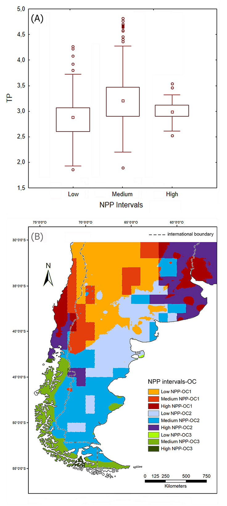
Figure 9. (A) Boxplot describing the distribution of trophic position (TP) values corresponding to the three net primary productivity (NPP) categories considered in this study; (B) map showing the geographical distribution of the nine variants resulting from combining the three NPP categories and the three omnivory categories considered in this study.

The most striking association found in this exploratory study is that between low levels of carnivory (OC I) and areas with low NPP values. The latter are located within the South American Arid Diagonal, a relatively stable natural physiographic unit. While absolute NPP values may have varied there over the last 4,000 years BP,⁵ it is virtually certain that they must have remained low throughout the entire late Holocene period. To explain the observed association between low levels of carnivory and low NPP values, we can resort to an adapted version of the trophic limitation hypothesis (cf. Kaspari, 2001), which states that an omnivorous vertebrate species occupying broad NPP gradients will show a predominance of lower trophic positions at low NPP, whereas individuals with a high degree of carnivory will be underrepresented at low NPP. This is because the more trophic links exist between NPP and consumers (i.e., the greater their degree of carnivory), the greater the energy required to maintain viable populations of those consumers. The reason for this is that the trophic biology of a species limits its ability to convert environmental productivity into more individuals of that species (Heal and MacLean Jr, 1975; Kaspari, 2001; Odum, 1971). This also relates to the aforementioned habitat productivity hypothesis, which posits that increased prey consumption by omnivores is facilitated by increased NPP, the latter understood as a measure of the amount of carbohydrates available in the ecosystem. It is the metabolism of such carbohydrates that provides the energy needed to sustain increased prey consumption by omnivores and the resulting increase in their biomass (Clay et al., 2017).

6.2 Effective temperature ranges

Effective temperature (ET) is a statistic that reflects the average temperature during the warmest and coldest months, as well as the length of the growing season of primary production (Bailey, 1960). In other words, ET measures both the length of the growing season and the intensity of solar energy available during it. Since biotic production is primarily driven by solar radiation, along with sufficient water to sustain photosynthesis, a general relationship between the value of ET and overall patterns of biotic activity and, consequently, production is expected (Binford, 1980).

Johnson (2014), based on data collected and modeled by Binford (2001), recognized six patterns of intensification⁶ in foragers economies. These patterns result from the combination of Binford's effective temperature (ET) thresholds (i.e., storage needed when ET < 15.25°C; plant reliance possible when ET ≥ 12.75°C) and the availability of sufficient aquatic resources for these to be an intensification option. Pattern 1 is characterized by wide ET ranges where mobile hunter-gatherers do not need food storage, could rely primarily on terrestrial plants, and aquatic resources are an intensification option. Pattern 2 presents ET ranges where mobile hunter-gatherers do not need storage, could rely primarily on plants, with plants being the only intensification option available. Pattern 3 occurs at mid-ranges of ET where mobile hunter-gatherers do need storage, could rely primarily on plants, and aquatic resources are an intensification option. Pattern 4 occurs at mid-ranges of ET where mobile hunter-gatherers need storage could rely primarily on plants, with these being the only intensification option. Pattern 5 is characterized by low ranges of ET where mobile hunter-gatherers would need substantial storage, could not rely primarily on plants, and aquatic resources are the only intensification option available. Pattern 6, finally, corresponds to low ET ranges where mobile hunter-gatherers would need substantial storage but could not rely primarily on terrestrial plants and aquatic resources are not an option for economic intensification. Trophic position values between 2 and 2.5 are expected in patterns 2 and 4, values between 2.5 and 3 are expected in patterns 1 and 3, while values higher than 3, revealing a higher degree of carnivory, are expected in patterns 5 and 6. In southern South America all patterns are represented except pattern 6 (see distribution map in Johnson, 2014).

As shown in Figure 9, the spatial structuring of OCs fits quite well with the expected distribution of subsistence patterns defined by Johnson (2014). In particular, the coincidence between the shape and extension of the area corresponding to patterns 4 and 2 (primary dependence on plant resources) and the main distribution areas of OC I is noteworthy. Something similar occurs with patterns 1 and 3 of the Binford-Johnson model (primary dependence on plant resources and aquatic resources as an intensification option), which coincide with the central-northern distribution of OC II, and pattern 5 (primary dependence on terrestrial and aquatic animals), which coincides with the southern distribution of OCII. For their part, the coastal areas where OC III is expressed are included within the zones corresponding to patterns 3 and 5, thus reflecting the importance of aquatic resources of marine origin. All this suggests that, at least, some variables of the Binfordian model based on environmental and hunter-gatherer frames of reference (Binford, 2001), as operationalized by Johnson (2014), have some explanatory power in relation to the situation described in our study.

Among foragers, cooking pottery is a key element of post-harvest intensification (Fuller and Champion, 2024). It is a technological device that enables not only the implementation of cooking methods (e.g., boiling) that make foods more edible and their nutrients more bioaccessible (Fuller and Champion, 2024), but also the transformation of perishable fresh products, such as fat, milk and fish, into longer-lasting products that can be stored or exchanged (Craig, 2021). In the study area, pottery is a widespread technology produced and used by foragers, agriculturalists and horticulturists alike. Although not in all cases its presence is associated with intensification processes (e.g., García, 2017), it is interesting to mention the cases of the northeast and southwest of Patagonia. In the first region (Valdés Peninsula), the results of BSIA and gas chromatography performed on organic residues found in ceramic sherds from different sites suggest that, around 1,500–1,000 years BP, pottery technology would have been linked to a process of intensification in the use of plants and fish (Gómez Otero et al., 2014). In the second region (west-center of Santa Cruz province), ceramic technology begins to appear in the archaeological record around 1,500 years BP, although a higher frequency of cases is observed—within a general context of scarcity of finds—around 900 years BP (Chaile et al., 2020). Based on BSIA and gas chromatography/gas chromatography coupled to mass spectrometry performed on organic residues found in ceramic sherds, it was established that pottery technology would have been used to process and preserve camelid (guanaco) fat (Chaile et al., 2020). These findings fit well with the expectations derived from patterns 3 and 5 of the Binford/Johnson model, although in the case of southwestern Patagonia, corresponding to an inland area far from the sea and with low freshwater fish diversity, intensification—if ever occurred (see Goñi et al., 2000-2002)—would have been based not on fish but on a more complete exploitation of the most common animal prey, the guanaco.

6.3 Differential distribution of marine biota

Although further studies are needed to obtain a more accurate estimate of the biodiversity of the Argentine Sea (Bigatti and Signorelli, 2018; Lutz et al., 2003), it can be said that it is characterized by a rich variety of mollusks, seabirds and mammals (Bigatti and Signorelli, 2018; Falabella et al., 2009; Lutz et al., 2003; Zárate, 2013). In the case of invertebrates (particularly arthropods) and fish, their current known biodiversity is lower than expected or lower than that recorded in other areas, due either to real differences in biodiversity or insufficient sampling (Bigatti and Signorelli, 2018; Lutz et al., 2003). It has been established that around 80 species of birds depend on marine habitats for both their reproduction and their feeding, while more than 40 species of marine mammals have been recorded in coastal and offshore waters (Falabella et al., 2009; Lutz et al., 2003). In particular, the study by Falabella et al. (2009) has shown that the annual activity of 16 species of marine top predators such as albatrosses, petrels, penguins, sea lions and elephant seals—although with seasonal variations—tends to concentrate in specific locations along the Patagonian coastline (Figure 10).

Figure 10

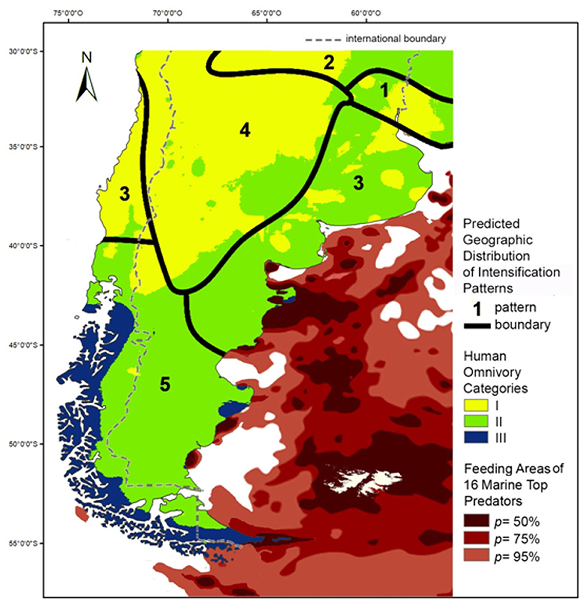
Figure 10. Superimposed maps of human omnivory categories, predicted distribution of intensificaction patterns described by Johnson (2014) and feeding areas of 16 marine top predators (redrawn from Falabella et al., 2009, correcting for differences in cartographic projection).

While there is evidence of prehistoric human exploitation of marine mammals, birds, mollusks and fishes along the entire Atlantic coast (e.g., Borrero and Barberena, 2006; Beretta and Zubimendi, 2019; Gómez Otero et al., 1998; Orquera and Gómez Otero, 2008; Scartascini, 2017; Zangrando and Tivoli, 2015), the highest TP values occur at three main areas projecting deep into the ocean, namely the Valdés Peninsula in northern Patagonia, the southern end of the Gulf of San Jorge in central Patagonia and the Miter Peninsula in Tierra del Fuego. As Figure 10 shows, these three areas are among the most used throughout the year by top predators, both birds and mammals (Falabella et al., 2009). In these areas, humans predate on other predators (e.g., sea lions, albatrosses, petrels, penguins) participating in complex food webs that derive their energy from marine BCSs, both pelagic and benthic. This is consistent with the aforementioned suggestion by Roopnarine (2014) that humans, in coastal marine environments, can behave as apex predators.

6.4 The spatial variation of human omnivory in the study area and the perfectible nature of maps

As can be seen from the preceding discussion, there are several factors that can contribute to varying degrees to explain the spatial patterns detected in this exploratory study. However, it is difficult to distinguish which of them are the most important, as they have confounding effects. This underscores the need to carry out macroecological analyses that allow going beyond pattern recognition addressing, in an integrated way, the identification and explanation of the underlying processes.

However, it is important to emphasize that the task of pattern recognition, one of the main objectives of this paper, is an activity that should not be stopped or abandoned. This is because maps, as models or representations, are perfectible constructs (Nguyen and Frigg, 2022). Among the key aspects that can be improved in map production is the estimation of the isotopic baseline used to derive TP. This estimate must take into account the different climatic conditions prevailing at different times in the late Holocene. This can be achieved, following the methodology described in Bowen and West (2008), by feeding a mass balance equation (Amundson et al., 2003) with paleoclimatic data, such as those available in the R-based program Pastclim 2.1 (Leonardi et al., 2023). Another important aspect to improve in our model, in line with the above, is the segmentation of the isotopic database into shorter time blocks. This will require finding an optimal solution to the problem of reducing the temporal dispersion of data without sacrificing spatial coverage, something that seems difficult to achieve given the current structure of the available dataset.

7 Concluding remarks

Isotopic and derived variable (e.g., TP) maps are powerful resources with redescriptive, comparative and heuristic value, as we try to demonstrate in this paper. It should be noted that, regardless of the performance of specific models like the one explored here, they are not intended nor desired to replace efforts to construct detailed isotopic ecologies at more restricted spatial scales or to carry out more standard analyses such as isotopic niche analysis or Bayesian isotopic mixing modeling. Quite the contrary, such studies provide relevant information for the interpretation of the maps. In any case, what is expected and considered beneficial for the advancement of archaeological and paleoecological studies focused on BSIA is a continuous interaction and feedback between this type of analysis and the spatial modeling of isotopic data. Although this contribution has not delved into this aspect due to its exploratory nature, we hope that it serves as an incentive for further development of this line of inquiry by other researchers.

Data availability statement

The original contributions presented in the study are included in the article/Supplementary material, further inquiries can be directed to the corresponding author.

Ethics statement

Ethical approval was not required for the study involving humans in accordance with the local legislation and institutional requirements. Written informed consent to participate in this study was not required from the participants or the participants' legal guardians/next of kin in accordance with the national legislation and the institutional requirements.

Author contributions

GB: Conceptualization, Formal analysis, Funding acquisition, Methodology, Project administration, Software, Supervision, Writing – original draft, Writing – review & editing. LC: Formal analysis, Funding acquisition, Methodology, Project administration, Software, Visualization, Writing – original draft, Writing – review & editing. NM: Data curation, Methodology, Software, Writing – original draft, Writing – review & editing.

Funding

The author(s) declare that financial support was received for the research and/or publication of this article. This research was partially funded by projects “Paisajes arqueológicos en las Sierras Australes de la Provincia de Buenos Aires: un estudio de los ambientes serranos, periserranos y de llanura. Tercera parte” (N1011-UNLP) and “La organización espacial de las sociedades cazadoras-recolectoras holocénicas del sudeste del espinal (provincia de Buenos Aires)” (N1062-UNLP).

Conflict of interest

The authors declare that the research was conducted in the absence of any commercial or financial relationships that could be construed as a potential conflict of interest.

Generative AI statement

The author(s) declare that no Gen AI was used in the creation of this manuscript.

Publisher's note

All claims expressed in this article are solely those of the authors and do not necessarily represent those of their affiliated organizations, or those of the publisher, the editors and the reviewers. Any product that may be evaluated in this article, or claim that may be made by its manufacturer, is not guaranteed or endorsed by the publisher.

Supplementary material

The Supplementary Material for this article can be found online at: https://www.frontiersin.org/articles/10.3389/fearc.2025.1521035/full#supplementary-material

Footnotes

1. ^The position of a species within a food web can be described by its fractional trophic level (FTL) (Pauly and Christensen, 2000) or by its trophic position (TP), the latter measured by stable isotopes of nitrogen (Post, 2002). In this paper we will refer mostly to TP.

2. ^The delta value (δ) is calculated as follows: δX = [(Rs / Rstd) - 1] ^* 1000, where δX is the delta value for the element X, Rs is the isotope ratio (e.g., ¹³C/¹²C) in the sample, and Rstd is the isotope ratio in the standard (Michener and Lajtha, 2007).

3. ^Some of the problems inherent in calculating TP with BSIA can currently be overcome, to some extent, by using compound-specific nitrogen isotope analysis of amino acids (CSIA-AA) (Ishikawa, 2018). However, for most archaeological samples this type of data is not yet available, so bulk collagen stable isotope data are still necessary in a study of the kind proposed here (Barrientos et al., 2020).

4. ^Data extracted from an ESRI ArcView Format layer downloaded in https://sage.nelson.wisc.edu/data-and-models/atlas-of-the-biosphere/mapping-the-biosphere/ecosystems/net-primary-productivity/ (Foley et al., 1996; Kucharik et al., 2000).

5. ^NPP is a dynamic variable that updates its values at each point in space over short periods of time due to inherently unstable factors like CO₂ concentration, precipitation, soil water content or air and soil temperatures (Hatfield et al., 2008).

6. ^Boserup (1965) conceptualized intensification as a mostly technologically mediated process of increasing the yields of a resource (or a set of resources) per unit of land in a context of population growth and increased competition for the exploitation of available resources.

References

Abraham, E. M., Rodríguez, M. D., Rubio, M. C., Guida-Johnson, B., Gomez, L., and Rubio, C. (2000). Disentangling the concept of “South American Arid Diagonal”. J. Arid Environ. 175:104089. doi: 10.1016/j.jaridenv.2019.104089

Crossref Full Text | Google Scholar

Ackerly, D. D. (2003). Community assembly, niche conservatism, and adaptive evolution in changing environments. Int. J. Plant Sci. 164, S165–S184. doi: 10.1086/368401

Crossref Full Text | Google Scholar

Albrecht, J., Bocherens, H., Hobson, K. A., Drucker, D. G., Sergiel, A., Swenson, J. E., et al. (2024). Trophic adaptation of large terrestrial omnivores to global change. bioRxiv [Preprint]. doi: 10.1101/2024.05.07.590891

Crossref Full Text | Google Scholar

Alfonso-Durruty, M., Misarti, N., and Troncoso, A. (2023). “The dietary impact of the Inka's political strategies in the Semi-Arid Region (30°-31°S. Lat) of northern Chile,” in Foodways of the Ancient Andes. Transforming Diet, Cuisine, and Society, eds. M. Alfonso-Durruty and D.E. Blom (Arizona: University of Arizona Press), 282–302. doi: 10.2307/j.ctv37xg2bh.17

Crossref Full Text | Google Scholar

Amundson, R., Austin, A. T., Schuur, E. A. G., Yoo, K., Matzek, V., Kendall, C., et al. (2003). Global patterns of the isotopic composition of soil and plant nitrogen. Global Biogeochem. Cycles. 17:1031. doi: 10.1029/2002GB001903

Crossref Full Text | Google Scholar

Anderson, C., and Cabana, G. (2007). Estimating the trophic position of aquatic consumers in river food webs using stable nitrogen isotopes. J. North Am. Benthol. Soc. 26, 273–285. doi: 10.1899/0887-3593(2007)26[273:ETTPOA]2.0.CO

Crossref Full Text | Google Scholar

Arim, M., Bozinovic, F., and Marquet, P. A. (2007a). On the relationship between trophic position, body mass and temperature: reformulating the energy limitation hypothesis. Oikos. 116, 1524–1530. doi: 10.1111/j.0030-1299.2007.15768.x

Crossref Full Text | Google Scholar

Arim, M., Marquet, P. A., and Jaksic, F. M. (2007b). On the relationship between productivity and food chain length at different ecological levels. Am. Nat. 169, 62–72. doi: 10.1086/510210

PubMed Abstract | Crossref Full Text | Google Scholar

Arnoldi, J.-F., Bortoluzzi, J. R., Rowland, H., Harrod, C., Parnell, A. C., Payne, N., et al. (2024). How strongly does diet variation explain variation in isotope values of animal consumers? PLoS ONE. 19:e0301900. doi: 10.1371/journal.pone.0301900

PubMed Abstract | Crossref Full Text | Google Scholar

Arora, S., Kataria, P., Nautiyal, M., Tuteja, I., Sharma, V., Ahmad, F., et al. (2023). Comprehensive review on the role of plant protein as a possible meat analogue: framing the future of meat. ACS omega. 8, 23305–23319. doi: 10.1021/acsomega.3c01373

PubMed Abstract | Crossref Full Text | Google Scholar

Bailey, H. P. (1960). A method of determining the warmth and temperateness of climate. Geogr. Ann. 42, 1–16. doi: 10.1080/20014422.1960.11880936

Crossref Full Text | Google Scholar

Baiser, B., Gravel, D., Cirtwill, A. R., Dunne, J. A., Fahimipour, A. K., Gilarranz, L. J., et al. (2019). Ecogeographical rules and the macroecology of food webs. Glob. Ecol. Biogeogr. 28, 1204–1218. doi: 10.1111/geb.12925

Crossref Full Text | Google Scholar

Banks-Leite, C., Betts, M. G., Ewers, R. M., Orme, C. D. L., and Pigot, A. L. (2022). The macroecology of landscape ecology. Trends Ecol. Evol. 37, 480–487. doi: 10.1016/j.tree.2022.01.005

PubMed Abstract | Crossref Full Text | Google Scholar

Barrientos, G., Catella, L., and Morales, N. S. (2020). A journey into the landscape of past feeding habits: Mapping geographic variations in the isotope (δ¹⁵N) -inferred trophic position of prehistoric human populations. Quat. Int. 548, 13–26. doi: 10.1016/j.quaint.2020.01.023

Crossref Full Text | Google Scholar

Battaglia Richi, E., Baumer, B., Conrad, B., Darioli, R., Schmid, A., and Keller, U. (2015). Health risks associated with meat consumption: a review of epidemiological studies. Int. J. Vitam. Nutr. Res. 85, 70–78. doi: 10.1024/0300-9831/a000224

PubMed Abstract | Crossref Full Text | Google Scholar

Bearhop, S., Adams, C. E., Waldron, S., Fuller, R. A., and Macleod, H. (2004). Determining trophic niche width: a novel approach using stable isotope analysis. J. Anim. Ecol. 73, 1007–1012. doi: 10.1111/j.0021-8790.2004.00861.x

Crossref Full Text | Google Scholar

Beaton, J. M. (1991). “Colonizing continents: some problems from Australia and the Americas,” in The First Americans: Search and Research, eds. T.D. Dillehay and D.J. Meltzer (Boca Raton: CRC Press), 209–230.

Google Scholar

Ben-Dor, M., Sirtoli, R., and Barkai, R. (2021). The evolution of the human trophic level during the Pleistocene. Am. J. Phys. Anthropol. 175, 27–56. doi: 10.1002/ajpa.24247

PubMed Abstract | Crossref Full Text | Google Scholar

Beretta, J. M., and Zubimendi, M. A. (2019). Explotación de avifauna en el sitio Cueva del Negro (Costa Norte de Santa Cruz). Mundo de Antes. 13, 85–112. doi: 10.59516/mda.v13.194

Crossref Full Text | Google Scholar

Berman, A. L., Silvestri, G. E., and Tonello, M. S. (2020). Paleoclimatic context of projected future warming in southern South America. Theor. Appl. Climatol. 141, 173–181. doi: 10.1007/s00704-020-03196-2

Crossref Full Text | Google Scholar

Bigatti, G., and Signorelli, J. H. (2018). Marine invertebrate biodiversity from the Argentine Sea, South Western Atlantic. ZooKeys 791, 47–70. doi: 10.3897/zookeys.791.22587

PubMed Abstract | Crossref Full Text | Google Scholar

Binford, L. R. (1980). Willow smoke and dogs' tails: Hunter-gatherer settlement systems and archaeological site formation. Am. Antiq. 45, 4–20. doi: 10.2307/279653

Crossref Full Text | Google Scholar

Binford, L. R. (2001). Constructing Frames of Reference: An Analytical Method for Archaeological Theory Building Using Ethnographic and Environmental Data Sets. Berkeley: University of California Press. doi: 10.1525/9780520925069

Crossref Full Text | Google Scholar

Blackburn, T. M., and Gaston, K. J. (2006). There's more to macroecology than meets the eye. Global. Ecol. Biogeogr. 15, 537–540. doi: 10.1111/j.1466-8238.2006.00276.x

Crossref Full Text | Google Scholar

Bocherens, H., and Drucker, D. (2003). Trophic level isotopic enrichment of carbon and nitrogen in bone collagen: case studies from recent and ancient terrestrial ecosystems. Int. J. Osteoarchaeol. 13, 46–53. doi: 10.1002/oa.662

Crossref Full Text | Google Scholar

Boecklen, W. J., Yarnes, C.h.T., Cook, B. A., and James, A.C. (2011). On the use of stable isotopes in trophic ecology. Annu. Rev. Ecol. Evol. Syst. 42, 411–440. doi: 10.1146/annurev-ecolsys-102209-144726

Crossref Full Text | Google Scholar

Bonhommeau, S., Dubroca, L., Le Pape, O., Barde, J., Kaplan, D. M., Chassot, E., et al. (2013). Eating up the world's food web and the human trophic level. PNAS 110, 20617–20620. doi: 10.1073/pnas.1305827110

PubMed Abstract | Crossref Full Text | Google Scholar

Borrero, L. A. (1994–1995). Arqueología de la Patagonia. Palimpsest. Rev. Arqueol. 4, 9–69.

Google Scholar

Borrero, L. A. (2001). “Cambios, continuidades, discontinuidades: discusiones sobre arqueología Fuego-Patagonia,” in Historia Prehispánica Argentina, vol. 2., eds. E.E. Berberián and A.E. Nielsen (Córdoba: Brujas), 815–838.

Google Scholar

Borrero, L. A., and Barberena, R. (2006). Hunter-Gatherer home ranges and marine resources. An archaeological case from Southern Patagonia. Curr. Anthropol. 47, 855–867. doi: 10.1086/507186

Crossref Full Text | Google Scholar

Boserup, E. (1965). The Conditions of Agricultural Growth: The Economics of Agrarian Change under Population Pressure. London: Allen and Unwin.

PubMed Abstract | Google Scholar

Bowen, G. J. (2010). “Statistical and geostatistical mapping of precipitation water isotope ratios,” in Isoscapes: Understanding Movement, Pattern, and Process on Earth through Isotope Mapping, eds. J.B. West, G.J. Bowen, K.P. Tu and T.E. Dawson (Dordrecht: Springer), 139–160. doi: 10.1007/978-90-481-3354-3_7

Crossref Full Text | Google Scholar

Bowen, G. J., and West, J. B. (2008). Isotope landscapes for terrestrial migration research. Track. Anim. Migrat. Stable Isot. 2, 79–105. doi: 10.1016/S1936-7961(07)00004-8

Crossref Full Text | Google Scholar

Bowen, G. J., West, J. B., Vaughn, B. H., Dawson, T. E., Ehleringer, J. R., Fogel, M. L., et al. (2009). Isoscapes to address large-scale Earth science challenges. Eos. 90, 109–110. doi: 10.1029/2009EO130001

Crossref Full Text | Google Scholar

Breed, M., and Moore, J. (2016). Animal Behavior, second ed. San Diego: Academic Press.

Google Scholar

Brown, D. A., and Pacheco, S. (2006). “Propuesta de actualización del mapa ecorregional de la Argentina,” in La Situación Ambiental Argentina 2005, eds. A. Brown, U. Martínez Ortiz, M. Acerbi and J. Corcuera (Buenos Aires: Fundación Vida Silvestre Argentina), 28–31.

Google Scholar

Brown, J. H., and Maurer, B. A. (1989). Macroecology: the division of food and space among species on continents. Science 243, 1145–1150. doi: 10.1126/science.243.4895.1145

PubMed Abstract | Crossref Full Text | Google Scholar

Bruniard, E. D. (1982). La diagonal árida argentina: un límite climático real. Rev. Geogr. 95, 5–20.

Google Scholar

Burkart, R., Bárbaro, N. O., Sánchez, R. O., and Gómez, D. A. (1999). Eco-Regiones de la Argentina. Buenos Aires: Administración de Parques Nacionales.

Google Scholar

Burness, G. P., Diamond, J., and Flannery, T. (2001). Dinosaurs, dragons, and dwarfs: the evolution of maximal body size. Proc. Natl. Acad. Sci. U.S.A. 98, 14518–14523. doi: 10.1073/pnas.251548698

PubMed Abstract | Crossref Full Text | Google Scholar

Burrough, P. A., and McDonnell, R. A. (1998). “Creating continuous surfaces from point data,” in Principles of Geographic Information Systems, eds. P.A. Burrough, M.F. Goodchild, R.A. McDonnell, P. Switzer and M. Worboys (Oxford: Oxford University Press), 132–161.

Google Scholar

Cabana, G., and Rasmussen, J. B. (1996). Comparison of aquatic food chains using nitrogen isotopes. Proc. Natl. Acad. Sci. U.S.A. 93, 10844–10847. doi: 10.1073/pnas.93.20.10844

PubMed Abstract | Crossref Full Text | Google Scholar

Cabrera, A. L., and Willink, A. (1973). Biogeografía de América Latina (Vol. 13). Washington DC: Programa Regional de Desarrollo Científico y Tecnológico.

Google Scholar

Casey, M. M., and Post, D. M. (2011). The problem of isotopic baseline: reconstructing the diet and trophic position of fossil animals. Earth Sci. Rev. 106, 131–148. doi: 10.1016/j.earscirev.2011.02.001

Crossref Full Text | Google Scholar

Castro, A., Gómez Otero, J., Arrigoni, G., and Moreno, E. (2004). “Prospección macrorregional comparativa a las loberías de la costa atlántica continental de Patagonia: algunas claves para el uso del espacio y de otros recursos,” in Contra Viento y Marea. Arqueología de la Patagonia, eds. T. Civalero, P. Fernández and A.G. Guraieb (Buenos Aires: Instituto Nacional de Antropología y Pensamiento Latinoamericano), 197–215.

Google Scholar

Catella, L., Barrientos, G., and Morales, N. S. (2018). La dimensión espacial de la información isotópica: patrones geográficos y ecológicos a gran escala en el cono sur de Sudamérica. Rev. Mus. La Plata. 3:28R.

Google Scholar

Caut, S., Angulo, E., and Courchamp, F. (2009). Variation in discrimination factors (Δ¹⁵N and Δ¹³C): the effect of diet isotopic values and applications for diet reconstruction. J. Appl. Ecol. 46, 443–453. doi: 10.1111/j.1365-2664.2009.01620.x

Crossref Full Text | Google Scholar

Chaile, C., Goñi, R. A., and Cassiodoro, G. E. (2020). “Uso de cerámica en cazadores-recolectores del centro-oeste de la provincia de Santa Cruz (Patagonia Argentina),” in Cerámica Arqueológica Patagonia, eds. V. Schuster and A.E. Pérez (Ciudad Autónoma de Buenos Aires: Fundación de Historia Natural Félix de Azara), 59–76.

Google Scholar

Chase, J. M., and Leibold, M. A. (2003). Ecological Niches. Linking Classical and Contemporary Approaches. Chicago: The University of Chicago Press. doi: 10.7208/chicago/9780226101811.001.0001

Crossref Full Text | Google Scholar

Chinique de Armas, Y. C., and Pestle, W. (2018). Assessing the association between subsistence strategies and the timing of weaning among indigenous archaeological populations of the Caribbean. Int. J. Osteoarchaeol. 28, 492–509. doi: 10.1002/oa.2695

Crossref Full Text | Google Scholar

Chubaty, A. M., Ma, B. O., Stein, R. W., Gillespie, D. R., Henry, L. M., Phelan, C., et al. (2013). On the evolution of omnivory in a community context. Ecol. Evol. 4, 1–15. doi: 10.1002/ece3.923

PubMed Abstract | Crossref Full Text | Google Scholar

Clare, E. L., Goerlitz, H. R., Drapeau, V. A., Holderied, M. W., Adams, A. M., Nagel, J., et al. (2014). Trophic niche flexibility in G lossophaga soricina: how a nectar seeker sneaks an insect snack. Funct. Eco. 28, 632–641. doi: 10.1111/1365-2435.12192

Crossref Full Text | Google Scholar

Clay, N. A., Lehrter, R. J., and Kaspari, M. (2017). Towards a geography of omnivory: omnivores increase carnivory when sodium is limiting. J. Anim. Ecol. 86, 1523–1531. doi: 10.1111/1365-2656.12754

PubMed Abstract | Crossref Full Text | Google Scholar

Closs, G. P., Balcombe, S. R., and Shirley, M. J. (1999). Generalist predators, interaction strength and food-web stability. Adv. Ecol. Res. 28, 93–126. doi: 10.1016/S0065-2504(08)60030-6

Crossref Full Text | Google Scholar

Coll, M., and Guershon, M. (2002). Omnivory in terrestrial arthropods: mixing plant and prey diets. Annu. Rev. Entomol. 47, 267–297. doi: 10.1146/annurev.ento.47.091201.145209

PubMed Abstract | Crossref Full Text | Google Scholar

Conolly, J., and Lake, M. (2006). Geographical Information Systems in Archaeology. Cambridge: Cambridge University Press. doi: 10.1017/CBO9780511807459

Crossref Full Text | Google Scholar

Crabtree, S. A., Vaughn, L. J. S., and Crabtree, N. T. (2017). Reconstructing Ancestral Pueblo food webs in the southwestern United States. J. Archaeol. Sci. 81, 116–127. doi: 10.1016/j.jas.2017.03.005

Crossref Full Text | Google Scholar

Craig, O. E. (2021). Prehistoric fermentation, delayed-return economies, and the adoption of pottery technology. Curr. Anthropol. 62, 233–241. doi: 10.1086/716610

Crossref Full Text | Google Scholar

Cucherousset, J., and Villéger, S. (2015). Quantifying the multiple facets of isotopic diversity: New metrics for stable isotope ecology. Ecol. Indic. 56, 152–160. doi: 10.1016/j.ecolind.2015.03.032

Crossref Full Text | Google Scholar

Cunningham, A. J., Worthington, S., Venkataraman, V. V., and Wrangham, R. W. (2019). Do modern hunter-gatherers live in marginal habitats? J. Archaeol. Sci. Rep. 25, 584–599. doi: 10.1016/j.jasrep.2019.05.028

Crossref Full Text | Google Scholar

Darimont, C. T., Cooke, R., Bourbonnais, M. L., Bryan, H. M., Carlson, S. M., Estes, J., et al. (2023). Humanity's diverse predatory niche and its ecological consequences. Commun. Biol. 6:609. doi: 10.1038/s42003-023-04940-w

PubMed Abstract | Crossref Full Text | Google Scholar

Darimont, C. T., Fox, C. H., Bryan, H. M., and Reimchen, T. E. (2015). The unique ecology of human predators. Science 349, 858–860. doi: 10.1126/science.aac4249

PubMed Abstract | Crossref Full Text | Google Scholar

de Martonne, E. (1935). Problèmes des régions arides sul-américaines. Ann. de Géog. 44, 1–27. doi: 10.3406/geo.1935.10784

Crossref Full Text | Google Scholar

DeNiro, M. J., and Epstein, S. (1981). Influence of diet on the distribution of nitrogen isotopes in animals. Geochem. Cosmochim. Acta. 45, 341–351. doi: 10.1016/0016-7037(81)90244-1

Crossref Full Text | Google Scholar

Diniz-Filho, J. A. F. (2023). The Macroecological Perspective. Cham: Springer. doi: 10.1007/978-3-031-44611-5

Crossref Full Text | Google Scholar

Elton, C. (1927). Animal Ecology. London: Sidgwick and Jackson.

Google Scholar

Erhardt, E., and Wilson, R. (2022). Foodweb trophic level and diet inference using an extended bayesian stable isotope mixing model. Open J. Ecol. 12, 333–359. doi: 10.4236/oje.2022.126020

Crossref Full Text | Google Scholar

Erlandson, J. M., and Fitzpatrick, S. M. (2006). Oceans, islands, and coasts: current perspectives on the role of the sea in human prehistory. J. Isl. Coast. Archaeol. 1, 5–32. doi: 10.1080/15564890600639504

Crossref Full Text | Google Scholar

Eubanks, M. D., and Denno, R. F. (2000). Host plants mediate omnivore–herbivore interactions and influence prey suppression. Ecology 81, 936–947. doi: 10.1890/0012-9658(2000)081[0936:HPMOHI]2.0.CO;2

Crossref Full Text | Google Scholar

Fairbridge, R. W., and Oliver, J. E. (1987). Maritime Climate, Oceanicity. Climatology. Encyclopedia of Earth Science. Boston: Springer.

Google Scholar

Falabella, F., Planella, M. T., and Tykot, R. H. (2008). El maíz (Zea mays) en el mundo prehispánico de Chile central. Latin Am. Antiq. 19, 25–46. doi: 10.1017/S1045663500007641

Crossref Full Text | Google Scholar

Falabella, V., Campagna, C., and Croxall, J. (2009). Atlas of the Patagonian Sea. Species and Spaces. Buenos Aires, Wildlife Conservation Society and BirdLife International. Available online at: http://www.atlas-marpatagonico.org (accessed September 15, 2024).

Google Scholar

Flaherty, E. A., and Ben-David, M. (2010). Overlap and partitioning of the ecological and isotopic niches. Oikos. 119, 1409–1416. doi: 10.1111/j.1600-0706.2010.18259.x

Crossref Full Text | Google Scholar

Foley, J. A., Prentice, I. C., Ramankutty, N., Levis, S., Pollard, D., Sitch, S., et al. (1996). An integrated biosphere model of land surface processes, terrestrial carbon balance, and vegetation dynamics. Global Biogeochem. Cycles. 10, 603–628. doi: 10.1029/96GB02692

Crossref Full Text | Google Scholar

Fuller, D. Q., and Champion, L. (2024). “Post-harvest intensification and “Pottery Pre-Neolithics': Endocuisine evolution in Asia and Africa from hunter-gatherers to early farmers,” in Early Pottery Technologies among Foragers in Global Perspective, eds. G. D'Ercole, E.A.A. Garcea, L. Varadzinová and L. Varadzin (Cham: Springer), 169–212. doi: 10.1007/978-3-031-71777-2_6

Crossref Full Text | Google Scholar

García, A. (2017). Intensificación económica y complejidad sociopolítica huarpe (centro-norte de Mendoza). Intersecc. Antropol. 18, 157–167.

Google Scholar

Garleff, K., and Stingl, H. (1998). Landschaftsentwicklung, Paläoökologie un Klimageschichte der Ariden Diagonaler Südamerikas im Jungquartär. Bamberg: Bamberger Geographische Schriften.

Google Scholar

Gastó, J., Cosio, F., and Panario, D. (1993). Clasificación de Ecorregiones y Determinación de Sitio y Condición. Manual de Aplicación a Municipios y Predios Rurales. Quito: Red de Pastizales Andinos.

Google Scholar

Gedeco Ltda (2008). Sistema de Clasificación de Ecorregiones. Gedeco Ltda., Santiago. Available online at: http://www.gedeco.cl/publicaciones/Review_SCE_Gedeco2008.pdf (accessed October 2, 2024).

PubMed Abstract | Google Scholar

Gil, A. F., Giardina, M. A., Neme, G. A., and Ugan, A. (2014). Demografía humana e incorporación de cultígenos en el centro occidente argentino: explorando tendencias en las fechas radiocarbónicas. Rev. Española Antropol. Am. 44, 523–533. Available online at: https://revistas.ucm.es/index.php/REAA/article/view/50728/47106

Google Scholar

Gil, A. F., Menéndez, L. P., Atencio, J. P., Peralta, E. A., Neme, G. A., et al. (2018). Estrategias humanas, estabilidad y cambio en la frontera agrícola sur americana. Latin Am. antiq. 29, 6–26. doi: 10.1017/laq.2017.59

Crossref Full Text | Google Scholar

Gil, A. F., Otaola, C., Dombrosky, J., Luna, M., Quiroga, G., and Dauverné, A. (2024). Dietary change of north patagonian guanacos: A historical ecology perspective through the study of stable isotopes. The Holocene. 34, 642–652. doi: 10.1177/09596836241231454

Crossref Full Text | Google Scholar

Goldfarb, G., and Sela, Y. (2023). The ideal diet for humans to sustainably feed the growing population - Review, meta-analyses, and policies for change. F1000Research 10:1135. doi: 10.12688/f1000research.73470.2

PubMed Abstract | Crossref Full Text | Google Scholar

Gómez Otero, J. (2007). Dieta, Uso del Espacio y Evolución en Poblaciones Cazadoras Recolectoras de la Costa Centro-Septentrional de Patagonia durante el Holoceno Medio y Tardío. [PhD Thesis]. [Ciudad Autónoma de Buenos Aires]: Universidad de Buenos Aires, Buenos Aires.

Google Scholar

Gómez Otero, J., Constenla, D. T., and Schuster, V. (2014). Isótopos estables de carbono y nitrógeno y cromatografía gaseosa en cerámica arqueológica del Nordeste de la provincia de Chubut (Patagonia Argentina). Arqueol. 20, 263–284. doi: 10.34096/arqueologia.t20.n2.1640

Crossref Full Text | Google Scholar

Gómez Otero, J., Lanata, J. L., and Prieto, A. (1998). Arqueología de la costa atlántica patagónica. Rev. Arqueol. Americana. 15, 107–185.

Google Scholar

Goñi, R., Barrientos, G., and Cassiodoro, G. (2000-2002). Las condiciones previas a la extinción de las poblaciones humanas del sur de Patagonia: una discusión a partir del análisis de la estructura del registro arqueológico de la cuenca del Lago Salitroso. Cuad. Inst. Nac. Antropol. Pensam. Latinoam. 19, 249–266. Available online at: https://revistas.inapl.gob.ar/index.php/cuadernos/article/view/546/315

Google Scholar

Guiry, E. J., and Szpak, P. (2021). Improved quality control criteria for stable carbon and nitrogen isotope measurements of ancient bone collagen. J. Archaeol. Sci. 132:105416. doi: 10.1016/j.jas.2021.105416

Crossref Full Text | Google Scholar

Gusinde, M. ([1937] 1986). Los Indios de Tierra del Fuego. Los Yámanas I-II-III. Buenos Aires: Consejo Nacional de Investigaciones Científicas.

Google Scholar

Gutgesell, M. K., McCann, K. S., Gellner, G., Cazelles, K., Greyson-Gaito, C.h.J., Bieg, C., et al. (2022). On the dynamic nature of omnivory in a changing world. BioScience 72, 416–430. doi: 10.1093/biosci/biab144

Crossref Full Text | Google Scholar

Hansson, S., Hobbie, J. E., Elmgren, R., Larsson, U., Fry, B., and Johansson, S. (1997). The stable nitrogen isotope ratio as a marker of food-web interactions and fish migration. Ecology 78, 2249–2257. doi: 10.1890/0012-9658(1997)078]2249:TSNIRA]2.0.CO;2

Crossref Full Text | Google Scholar

Hatfield, J. L., Boote, K. J., Fay, P., Hahn, L., Izaurralde, C., Kimball, B. A., et al. (2008). “Agriculture,” in The Effects of Climate Change on Agriculture, Land Resources, Water Resources, and Biodiversity in the United States, ed. M. Walsh (Washington: U.S. Climate Change Science Program and the Subcommittee on Global Change Research), 21–74.

Google Scholar

Heal, O. W., and MacLean Jr, S. F. (1975). “Comparative productivity in ecosystems—secondary productivity,” in Unifying Concepts in Ecology: Report of the Plenary Sessions of the First International Congress of Ecology, eds. W.H. Dobben and R.H. Lowe-McConnell (Dordrecht: Springer), 89–108. doi: 10.1007/978-94-010-1954-5_8

Crossref Full Text | Google Scholar

Hedges, R. E. M., and Reynard, L. M. (2007). Nitrogen isotopes and the trophic level of humans in archaeology. J. Archaeol. Sci. 34, 1240–1251. doi: 10.1016/j.jas.2006.10.015

Crossref Full Text | Google Scholar

Hengl, T. (2007). A Practical Guide to Geostatistical Mapping of Environmental Variables. Luxemburg: European Communities.

Google Scholar

Hermes, T. R., Frachetti, M. D., Bullion, E. A., Maksudov, F., Mustafokulov, S., Makarewicz, C.h., et al. (2018). Urban and nomadic isotopic niches reveal dietary connectivities along Central Asia's Silk Roads. Sci. Rep. 8:5177. doi: 10.1038/s41598-018-22995-2

PubMed Abstract | Crossref Full Text | Google Scholar

Hette-Tronquart, N. (2019). Isotopic niche is not equal to trophic niche. Ecol. Lett. 22, 1987–1989. doi: 10.1111/ele.13218

PubMed Abstract | Crossref Full Text | Google Scholar

Hobson, K. A., and Clark, R. G. (1992). Assessing avian diets using stable isotopes ii: factors influencing diet-tissue fractionation. Condor 94, 189–197. doi: 10.2307/1368808

Crossref Full Text | Google Scholar

Holland, J. N., and DeAngelis, D. L. (2010). A consumer–resource approach to the density-dependent population dynamics of mutualism. Ecology 91, 1286–1295. doi: 10.1890/09-1163.1

PubMed Abstract | Crossref Full Text | Google Scholar

Hopkins J. B. III. and Kurle C. M. (2016). Measuring the realized niches of animals using stable isotopes: from rats to bears. Methods Ecol. Evol. 7, 210–221. doi: 10.1111/2041-210X.12446

Crossref Full Text | Google Scholar

Ichikawa, M., Hattori, S., and Yasuoka, H. (2011). “5 environmental knowledge among central african hunter-gatherers: types of knowledge and intra-cultural variations,” in Information and Its Role in Hunter-Gatherer Bands, eds. R. Whallon, W.A. Lovis and R.K. Hitchcock (Los Ángeles: Cotsen Institute of Archaeology Press at UCLA), 117–132. doi: 10.2307/j.ctvdmwwz4.9

Crossref Full Text | Google Scholar

Ishikawa, N. F. (2018). Use of compound-specific nitrogen isotope analysis of amino acids in trophic ecology: assumptions, applications, and implications. Ecol. Res. 33, 825–837. doi: 10.1007/s11284-018-1616-y

Crossref Full Text | Google Scholar

Jackson, A. L., Inger, R., Parnell, A. C., and Bearhop, S. (2011). Comparing isotopic niche widths among and within communities: SIBER – Stable Isotope Bayesian Ellipses in R. J. Anim. Ecol. 80, 95–602. doi: 10.1111/j.1365-2656.2011.01806.x

PubMed Abstract | Crossref Full Text | Google Scholar

Jacquier, M., Vandel, J.-M., Léger, F., Duhayer, J., Pardonnet, S., Say, L., et al. (2021). Breaking down population density into different components to better understand its spatial variation. BMC Ecol. Evol. 21:82. doi: 10.1186/s12862-021-01809-6

PubMed Abstract | Crossref Full Text | Google Scholar

Johnson, A. L. (2014). Exploring adaptive variation among hunter-gatherers with Binford's frames of reference. J. Archaeol. Res. 22, 1–42. doi: 10.1007/s10814-013-9068-y

Crossref Full Text | Google Scholar

Kaspari, M. (2001). Taxonomic level, trophic biology and the regulation of local abundance. Global Ecol. Biogeogr. 10, 229–244. doi: 10.1046/j.1466-822X.2001.00214.x

Crossref Full Text | Google Scholar

Keough, J. R., Sierszen, M. E., and Hagley, C. A. (1996). Analysis of a Lake Superior coastal food web with stable isotope techniques. Limnol. Oceanogr. 41, 136–146. doi: 10.4319/lo.1996.41.1.0136

Crossref Full Text | Google Scholar

Knapp, A. K., Carroll, C. J. W., and Fahey, T. J. (2014). “Primary production in terrestrial ecosystems: Patterns and controls in a changing world,” in Ecology and the Environment, ed. R. Monson (New York: Springer), 1–36. doi: 10.1007/978-1-4614-7612-2_2-1

Crossref Full Text | Google Scholar

Kochi, S., Gómez Otero, J., Zangrando, A. F., Tessone, A., and Ugan, A. (2024). Paleodiets of hunter-gatherers from the central Patagonian coast: reviewing scopes and limitations of stable isotope analyses. Int. J. Osteoarchaeol. 34:e3243. doi: 10.1002/oa.3243

Crossref Full Text | Google Scholar

Kochi, S., Pérez, S. A., Tessone, A., Ugan, A., Tafuri, M. A., Nye, J., et al. (2018). δ¹³C and δ¹⁵N variations in terrestrial and marine foodwebs of Beagle Channel in the Holocene. Implications for human paleodietary reconstructions. J. Archaeol. Sci. Rep. 18, 696–707. doi: 10.1016/j.jasrep.2017.11.036

Crossref Full Text | Google Scholar

Kraft, R., Jahren, A., and Saudek, C. (2008). Clinical-scale investigation of stable isotopes in human blood: ¹³C and ¹⁵N from 406 patients at the Johns Hopkins Medical Institution. Rapid Commun. Mass Spectrom. 22, 3683–3692. doi: 10.1002/rcm.3780

PubMed Abstract | Crossref Full Text | Google Scholar

Kucharik, C. J., Foley, J. A., Delire, C., Fisher, V. A., Coe, M. T., Lenters, J. D., et al. (2000). Testing the performance of a dynamic global ecosystem model: water balance, carbon balance, and vegetation structure. Global Biogeochem. Cycles. 14, 795–825. doi: 10.1029/1999GB001138

Crossref Full Text | Google Scholar

Layman, C. A., Araujo, M. S., Boucek, R., Hammerschlag-Peyer, C. M., Harrison, E., Jud, Z. R., et al. (2012). Applying stable isotopes to examine food-web structure: an overview of analytical tools. Biol. Rev. 87, 545–562. doi: 10.1111/j.1469-185X.2011.00208.x

PubMed Abstract | Crossref Full Text | Google Scholar

Layman, C. A., Arrington, D. A., Montaña, C. G., and Post, D. M. (2007). Can stable isotope ratios provide for community-wide measures of trophic structure? Ecology 88, 42–48. doi: 10.1890/0012-9658(2007)88[42:CSIRPF]2.0.CO;2

Crossref Full Text | Google Scholar

Lema, V., Della Negra, C., and Bernal, V. (2012). Explotación de recursos vegetales silvestres y domesticados en Neuquén: implicancias del hallazgo de restos de maíz y algarrobo en artefactos de molienda del Holoceno Tardío. Magallania. 40, 229–247. doi: 10.4067/S0718-22442012000100013

PubMed Abstract | Crossref Full Text | Google Scholar

Lennox, R. J., Brownscombe, J. W., Darimont, C., Horodysky, A., Levi, T., Raby, G. D., et al. (2022). The roles of humans and apex predators in sustaining ecosystem structure and function: Contrast, complementarity and coexistence. People Nat. 4, 1071–1082. doi: 10.1002/pan3.10385

Crossref Full Text | Google Scholar

Leonardi, M., Hallett, E. Y., Beyer, R., Krapp, M., and Manica, A. (2023). pastclim 1.2: an R package to easily access and use paleoclimatic reconstructions. Ecography 3:e06481. doi: 10.1111/ecog.06481

Crossref Full Text | Google Scholar

Leroy, F., Smith, N. W., Adesogan, A. T., Beal, T., Iannotti, L., Moughan, P. J., et al. (2023). The role of meat in the human diet: evolutionary aspects and nutritional value. Anim. Front. 13, 11–18. doi: 10.1093/af/vfac093

PubMed Abstract | Crossref Full Text | Google Scholar

Levine, S. (1980). Several measures of trophic structure applicable to complex food webs. J. Theor. Biol. 83, 195–207. doi: 10.1016/0022-5193(80)90288-X

Crossref Full Text | Google Scholar

Lewis, M. C., and Sealy, J. C. (2018). Coastal complexity: ancient human diets inferred from Bayesian stable isotope mixing models and a primate analogue. PLoS ONE 13:e0209411. doi: 10.1371/journal.pone.0209411

PubMed Abstract | Crossref Full Text | Google Scholar

Li, J., and Heap, A. D. (2008). A Review of Spatial Interpolation Methods for Environmental Scientists. Canberra: Geoscience Australia.

Google Scholar

Li, Z. (2021). An enhanced dual IDW method for high-quality geospatial interpolation. Sci. Rep. 11:9903. doi: 10.1038/s41598-021-89172-w

PubMed Abstract | Crossref Full Text | Google Scholar

Li, Z., Zhang, X., Zhu, R., Zhang, Z., and Weng, Z. (2019). Integrating data-to-data correlation into inverse distance weighting. Comput. Geosci. 24, 203–216. doi: 10.1007/s10596-019-09913-9

PubMed Abstract | Crossref Full Text | Google Scholar

Liman, A. S., Dalin, P., and Björkman, C. (2017). Enhanced leaf nitrogen status stabilizes omnivore population density. Oecologia 183, 57–65. doi: 10.1007/s00442-016-3742-y

PubMed Abstract | Crossref Full Text | Google Scholar

López, M. L., Berón, M., Prates, L., Medina, M., Heider, G., and Pastor, S. (2020). Las plantas en la alimentación de pueblos originarios de la diagonal árida argentina: Sierras Centrales, Pampa Seca y Norpatagonia. RIVAR 7, 81–102. doi: 10.35588/rivar.v7i21.4639

Crossref Full Text | Google Scholar

Loponte, D., and Acosta, A. (2013). La construcción de la unidad arqueológica guaraní en el extremo meridional de su distribución geográfica. Cuad. Inst. Nac. Antropol. Pensam. Latinoam. Ser. Espec. 1, 193–235. Available online at: https://revistas.inapl.gob.ar/index.php/series_especiales/article/view/1644

Google Scholar

Loponte, D., and Corriale, M. J. (2020). Patterns of Resource Use and Isotopic Niche Overlap Among Guanaco (Lama guanicoe), Pampas Deer (Ozotoceros bezoarticus) and Marsh Deer (Blastocerus dichotomus) in the Pampas. Ecological, Paleoenvironmental and Archaeological Implications. Environ. Archaeol. 25, 411–444. doi: 10.1080/14614103.2019.1585646

Crossref Full Text | Google Scholar

Lunghi, E., Cianferoni, F., Ceccolini, F., Veith, M., Manenti, R., Mancinelli, G., et al. (2018). What shapes the trophic niche of European plethodontid salamanders? PLoS ONE 13:e0205672. doi: 10.1371/journal.pone.0205672

PubMed Abstract | Crossref Full Text | Google Scholar

Lüning, S., Galka, M., Bamonte, F. P., García Rodríguez, F., and Vahrenholt, F. (2019). The medieval climate anomaly in South America. Quat. Int. 508, 70–87. doi: 10.1016/j.quaint.2018.10.041

Crossref Full Text | Google Scholar

Lutz, V. A., Boschi, E. E., Bremec, C. S., Cousseau, M. B., Figueroa, D. E., Rodríguez, D. H., et al. (2003). Perspectives of marine biodiversity studies in Argentina. Gayana. 67, 371–382. doi: 10.4067/S0717-65382003000200016

PubMed Abstract | Crossref Full Text | Google Scholar

MacPhee, R. D. E. (2009). “Insulae infortunatae: establishing a chronology for late quaternary mammal extinctions in the west Indies,” in American Megafaunal Extinctions at the End of the Pleistocene. Vertebrate Paleobiology and Paleoanthropology, ed. G. Haynes (Dordrecht: Springer), 169–193. doi: 10.1007/978-1-4020-8793-6_9

Crossref Full Text | Google Scholar

Maksic, J., Shimizu, M. H., de Oliveira, G. S., Venancio, I. M., Cardoso, M., and Ferreira, F. A. (2018). Simulation of the Holocene climate over South America and impacts on the vegetation. The Holocene. 29, 287–299. doi: 10.1177/0959683618810406

Crossref Full Text | Google Scholar

Mancini, M. V., Paez, M. M., Prieto, A. R., Stutz, S., Tonello, M., and Vilanova, I. (2005). Mid-Holocene climatic variability reconstruction from pollen records (32°-52°S, Argentina). Quat. Int. 132, 47–59. doi: 10.1016/j.quaint.2004.07.013

Crossref Full Text | Google Scholar

Marshall, H. H., Inger, R., Jackson, A. L., McDonald, R. A., Thompson, F. J., and Cant, M. A. (2019). Stable isotopes are quantitative indicators of trophic niche. Ecol. Lett. 22, 1990–1992. doi: 10.1111/ele.13374

PubMed Abstract | Crossref Full Text | Google Scholar

McCue, M. D., and Pollock, E. D. (2008). Stable isotopes may provide evidence for starvation in reptiles. Rapid Commun. Mass Spectrom. 22, 2307–2314. doi: 10.1002/rcm.3615

PubMed Abstract | Crossref Full Text | Google Scholar

McCutchan, J. H., Lewis, W. M., and McGrath, C. C. (2003). Variation in trophic shift for stable isotope ratios of carbon, nitrogen, and sulfur. Oikos. 102, 378–390. doi: 10.1034/j.1600-0706.2003.12098.x

PubMed Abstract | Crossref Full Text | Google Scholar

McEwan, C., Borrero, L., and Prieto, A. (1997). Patagonia. Natural History, Prehistory and Ethnography at the Uttermost end of the Earth. London: British Museum Press. doi: 10.1515/9781400864768

Crossref Full Text | Google Scholar

Michener, R., and Lajtha, K. (2007). Stable Isotopes in Ecology and Environmental Science. Ecological Methods and Concepts Series. Malden: Wiley/Blackwell. doi: 10.1002/9780470691854

Crossref Full Text | Google Scholar

Moosmann, M., Cuenca-Cambronero, M., De Lisle, S., Greenway, R., Hudson, C. M., Lürig, M. D., et al. (2021). On the evolution of trophic position. Ecol. Lett. 24, 2549–2562. doi: 10.1111/ele.13888

PubMed Abstract | Crossref Full Text | Google Scholar

Morello, J. (1984). Perfil Ecológico de Sudamérica. Características Estructurales de Sudamérica y su Relación con Espacios Semejantes del Planeta. Barcelona: Ediciones Cultura Hispánica - ICI.

Google Scholar

Morello, J., Matteucci, S. D. A., Rodríguez, F., and Silva, M. E. (2012). Ecorregiones y Complejos Ecosistémicos Argentinos. Buenos Aires: Editorial Orientación Gráfica Argentina.

Google Scholar

Morrone, J. J. (2015). Biogeographical regionalisation of the world: a reappraisal. Aust. Syst. Bot. 28, 81–90. doi: 10.1071/SB14042

Crossref Full Text | Google Scholar

Musaubach, M. G., and Berón, M. A. (2012). Food residues as indicators of processed plants in hunter-gatherers' pottery from La Pampa (Argentina). Veg. Hist. Archaeobotany. 26, 111–123. doi: 10.1007/s00334-016-0581-z

Crossref Full Text | Google Scholar

Myers, D. E. (1994). Spatial interpolation: an overview. Geoderma 62, 17–28. doi: 10.1016/0016-7061(94)90025-6

Crossref Full Text | Google Scholar

Nash, S. H., Kristal, A. R., Boyer, B. B., King, I. B., Metzgar, J. S., and O'Brien, D. M. (2009). Relation between stable isotope ratios in human red blood cells and hair: implications for using the nitrogen isotope ratio of hair as a biomarker of eicosapentaenoic acid and docosahexaenoic acid. Am. J. Clin. Nutr. 90, 1642–1647. doi: 10.3945/ajcn.2009.28482

PubMed Abstract | Crossref Full Text | Google Scholar

Neme, G. A. (2007). Cazadores-recolectores de altura en los Andes meridionales: en alto valle del río Atuel, Argentina (Vol. 1591). Oxford: BAR International Series Archaeopress. doi: 10.30861/9781407300078

Crossref Full Text | Google Scholar

Newsome, S. D., Martinez del Rio, C., Bearhop, S., and Phillips, D. L. (2007). A niche for isotopic ecology. Front. Ecol. Environ. 5, 429–436. doi: 10.1890/1540-9295(2007)5[429:ANFIE]2.0.CO;2

Crossref Full Text | Google Scholar

Newsome, S. D., Yeakel, J. D., Wheatley, P. V., and Tinker, M. T. (2012). Tools for quantifying isotopic niche space and dietary variation at the individual and population level. J. Mammal. 93, 329–341. doi: 10.1644/11-MAMM-S-187.1

Crossref Full Text | Google Scholar

Nguyen, J., and Frigg, R. (2022). Scientific Representation. Cambridge: Cambridge University Press. doi: 10.1017/9781009003575

Crossref Full Text | Google Scholar

Nieblas, A.-E., Bonhommeau, S., Le Pape, O., Chassot, E., Dubroca, L., Barde, J., et al. (2014). Reply to Roopnarine: what is an apex predator? PNAS 111:E797. doi: 10.1073/pnas.1324146111

PubMed Abstract | Crossref Full Text | Google Scholar

O'Connell, T. C., and Hedges, R. E. M. (1999). Investigations into the effect of diet on modern human hair isotopic values. Am. J. Phys. Anthropol. 108, 409–425. doi: 10.1002/(SICI)1096-8644(199904)108:4<409::AID-AJPA3>3.0.CO;2-E

Crossref Full Text | Google Scholar

O'Connell, T. C., Hedges, R. E. M., Healey, M. A., and Simpson, A. H. R. W. (2001). Isotopic comparison of hair, bone and nail: modern analyses. J. Archaeol. Sci. 28, 1247–1255. doi: 10.1006/jasc.2001.0698

Crossref Full Text | Google Scholar

O'Connell, T. C., Kneale, C. J., Tasevska, N., and Kuhnle, G. G. C. (2012). The diet-body offset in human nitrogen isotopic values: a controlled dietary study. Am. J. Phys. Anthropol. 149, 426–434. doi: 10.1002/ajpa.22140

PubMed Abstract | Crossref Full Text | Google Scholar

Odum, W. E. (1971). Pathways of Energy Flow in a South Florida Estuary. [PhD Thesis]. [Coral Gables (FL)]: University of Miami.

Google Scholar

Olalla-Tárraga, M. Á., González-Suárez, M., Bernardo-Madrid, R., Revilla, E., and Villalobos, F. (2017). Contrasting evidence of phylogenetic trophic niche conservatism in mammals worldwide. J. Biogeogr. 44, 99–110. doi: 10.1111/jbi.12823

Crossref Full Text | Google Scholar

Olson, D. M., Dinerstein, E., Wikramanayake, E. D., Burgess, N. D., Powell, G. V. N., Underwood, E. C., et al. (2001). Terrestrial Ecoregions of the World: A New Map of Life on Earth: a new global map of terrestrial ecoregions provides an innovative tool for conserving biodiversity. BioScience 51, 933–938. doi: 10.1641/0006-3568(2001)051[0933:TEOTWA]2.0.CO;2

Crossref Full Text | Google Scholar

Orquera, L. A., and Gómez Otero, J. (2008). Los cazadores-recolectores de las costas de Pampa, Patagonia y Tierra del Fuego. Relac. Soc. Argent. Antropol. 32, 75–99. Available online at: https://www.saantropologia.com.ar/wp-content/uploads/2015/01/Relaciones%2032/04%20Orquera-Gomez%20Otero.pdf

Google Scholar

Orquera, L. A., and Piana, E. L. (1999). La Vida Social y Material de los Yámana. Buenos Aires: Eudeba-IFIC.

Google Scholar

Oyarzabal, M., Clavijo, J., Oakley, L., Biganzoli, F., Tognetti, P., Barberis, I., et al. (2018). Unidades de vegetación de la Argentina. Ecol. Austral. 28, 40–63. doi: 10.25260/EA.18.28.1.0.399

PubMed Abstract | Crossref Full Text | Google Scholar

Pardo, L. H., and Nadelhoffer, J. (2010). “Using nitrogen isotope ratios to assess terrestrial ecosystems at regional and global scales,” in Isoscapes: Understanding Movement, Pattern, and Process on Earth through Isotope Mapping, eds. J. West, G. Bowen, T. Dawson and K. Tu (Dordrecht: Springer), 221–249. doi: 10.1007/978-90-481-3354-3_11

Crossref Full Text | Google Scholar

Pastor, S., and Gil, A. F. (2014). Variabilidad en las trayectorias de adopción de la agricultura en el sur de Sudamérica. Rev. Española Antropol. Am. 12, 453–464. Available online at: https://revistas.ucm.es/index.php/REAA/article/view/50725

Google Scholar

Pastor, S., and López, L. (2010). “Consideraciones sobre la agricultura prehispánica en el sector central de las Sierras de Córdoba (Argentina),” in Arqueología de la Agricultura: Casos de Estudio en la Región Andina Argentina, eds. A. Korstanje and M. Quesada (Tucumán: Editorial Magna), 208–233.

Google Scholar

Pate, D., and Schoeninger, M. (1993). “Stable carbon isotope ratios in bone collagen as indicators of marine and terrestrial dietary composition in southeastern Australia: a preliminary report,” in Archaeometry: Current Australasian Research, eds. B.L. Frankhauser and J.R. Bird (Canberra: Australian National University), 38–44.

Google Scholar

Pauly, D., and Christensen, V. (2000). “Trophic levels of fishes,” in Fishbase 2000: Concepts, Design and Data Sources, eds. R. Froese and D. Pauly (Manila: ICLARM), 181.

Google Scholar

Pearre, S. J. (1999). What's in a niche? II. Responses of trophic niche indices to simulated and actual prey distributions and sampling regimes. Evolut. Theory 12, 23–37.

Google Scholar

Peterson, B. J., Howarth, R. W., and Garritt, R. H. (1985). Multiple stable isotopes used to trace the flow of organic matter in estuarine food webs. Science 227, 1361–1363. doi: 10.1126/science.227.4692.1361

PubMed Abstract | Crossref Full Text | Google Scholar

Pezo-Lanfranco, L., Mut, P., Chávez, J., Fossile, T., Colonese, A. C., and Fernandes, R. (2024). South American Archaeological Isotopic Database, a regional-scale multi-isotope data compendium for research. Sci. Data. 11:336. doi: 10.1038/s41597-024-03148-9

PubMed Abstract | Crossref Full Text | Google Scholar

Pielou, E. C. (1979). Biogeography. New York: Wiley.

Google Scholar

Pimm, S. L., and Lawton, J. H. (1978). On feeding on more than one trophic level. Nature 275, 542–544. doi: 10.1038/275542a0

Crossref Full Text | Google Scholar

Pineau, V., Zangrando, A. F. J., Scheinsohn, V., Mondini, M., Fernández, P., Barberena, R., et al. (2003). “Las particularidades de Sudamérica y sus implicaciones para el proceso de dispersión de Homo sapiens,” in Análisis, Interpretación y Gestión en la Arqueología de Sudamérica, eds. R. Curtoni and M. L. Endere (Olavarría: INCUAPA-UNICEN), 121–133.

Google Scholar

Pineda-Munoz, S., and Alroy, J. (2014). Dietary characterization of terrestrial mammals. Proc. Biol. Sci. 281:20141173. doi: 10.1098/rspb.2014.1173

PubMed Abstract | Crossref Full Text | Google Scholar

Polis, G. A., Myers, C. A., and Holt, R. D. (1989). The ecology and evolution of intraguild predation: potential competitors that eat each other. Annu. Rev. Ecol. Evol. Syst. 20, 297–330. doi: 10.1146/annurev.es.20.110189.001501

PubMed Abstract | Crossref Full Text | Google Scholar

Polis, G. A., and Strong, D. R. (1996). Food web complexity and community dynamics. Am. Nat. 147, 813–846. doi: 10.1086/285880

Crossref Full Text | Google Scholar

Politis, G. (2008). “The pampas and campos of South America,” in Handbook of South American Archaeology, eds. H. Silverman and W. Isbell (New York: Springer), 235–260. doi: 10.1007/978-0-387-74907-5_14

Crossref Full Text | Google Scholar

Politis, G., and Bonomo, M. (2012). La entidad arqueológica Goya-Malabrigo (Ríos Paraná y Uruguay) y su filiación Arawak. Bol. Soc. Arqueol. Bras. 25, 10–48. doi: 10.24885/sab.v25i1.338

Crossref Full Text | Google Scholar

Politis, G. G., and Borrero, L. A. (2024). The Archaeology of the Pampas and Patagonia. Cambridge: Cambridge University Press. doi: 10.1017/9780511993251

Crossref Full Text | Google Scholar

Pollard, M. D., and Puckett, E. E. (2022). Evolution of degrees of carnivory and dietary specialization across Mammalia and their effects on speciation. bioRxiv [Preprint]. doi: 10.1101/2021.09.15.460515

Crossref Full Text | Google Scholar

Porter, C. C., and Marlowe, F. W. (2007). How marginal are forager habitats? J. Archaeol. Sci. 34, 59–68. doi: 10.1016/j.jas.2006.03.014

Crossref Full Text | Google Scholar

Post, D. M. (2002). Using stable isotopes to estimate trophic position: models, methods, and assumptions. Ecology 83, 703–718. doi: 10.1890/0012-9658(2002)083[0703:USITET]2.0.CO;2

PubMed Abstract | Crossref Full Text | Google Scholar

Powell, R. L., and Still, C. J. (2009). “Biogeography of C₃ and C₄ vegetation in South America,” in Anais XIV Simpósio Brasileiro de Sensoriamento Remoto, 2935–2942.

Google Scholar

Powell, R. L., Yoo, E., and Still, C. J. (2012). Vegetation and soil carbon-13 isoscapes for South America: integrating remote sensing and ecosystem isotope measurements. Ecosphere 3:109. doi: 10.1890/ES12-00162.1

Crossref Full Text | Google Scholar

Prates, L., Serna, A., Mange, E., López, L., Romano, V., Di Lorenzo, M., et al. (2019). Ocupaciones residenciales y entierros humanos en Negro Muerto 3 (Valle del Río Negro, Norpatagonia). Magallania 47, 159–176. doi: 10.4067/S0718-22442019000100159

PubMed Abstract | Crossref Full Text | Google Scholar

Pratte, I., Braune, B. M., Hobson, K. A., and Mallory, M. L. (2019). Variable sea-ice conditions influence trophic dynamics in an Arctic community of marine top predators. Ecol. Evol. 9, 7639–7651. doi: 10.1002/ece3.5313

PubMed Abstract | Crossref Full Text | Google Scholar

Pyrcz, M. J., and Deutsch, C. V. (2002). “Debiasing for improved inference of the one point statistic,” in Proceedings of the 30th International APCOM Symposium, ed. S. Bandopadhyay (Littleton: Society for Mining, Metallurgy, and Exploration), 251–260.

Google Scholar

Pyrcz, M. J., and Deutsch, C. V. (2014). Geostatistical Reservoir Modeling. Oxford: Oxford University Press.

Google Scholar

Reuter, D. M., Hopkins, S. S., and Price, S. A. (2023). What is a mammalian omnivore? Insights into terrestrial mammalian diet diversity, body mass and evolution. Proc. R. Soc. B. 290:20221062. doi: 10.1098/rspb.2022.1062

PubMed Abstract | Crossref Full Text | Google Scholar

Reyes, O., Tessone, A., San Román, M., and Méndez, C. (2019). Dieta e isótopos estables de cazadores recolectores marinos en los canales occidentales de Patagonia, Chile. Latin Am. Antiq. 30, 550–568. doi: 10.1017/laq.2019.40

Crossref Full Text | Google Scholar

Richards, M. P. (2006). “Palaeodietary reconstruction,” in St Martin's Uncovered: Investigations in the Churchyard of St Martin's-in-the-Bull Ring, Birmingham, eds. M. Brickley, S. Buteux, J. Adams, R. Cherrington (Oxford: Oxbow Books), 147–151.

Google Scholar

Robinson, J. T. (2021). Investigating isotopic niche space: using rKIN for stable isotope studies in archaeology. J. Archaeol. Method Theory 29, 831–861. doi: 10.1007/s10816-021-09541-7

Crossref Full Text | Google Scholar

Rodríguez, M. A. M., and Herrera, L. M. G. (2013). Isotopic niche mirrors trophic niche in a vertebrate island invader. Oecologia 171, 537–544. doi: 10.1007/s00442-012-2423-8

PubMed Abstract | Crossref Full Text | Google Scholar

Roopnarine, P. D. (2014). Humans are apex predators. PNAS 111:E796. doi: 10.1073/pnas.1323645111

PubMed Abstract | Crossref Full Text | Google Scholar

Root-Bernstein, M., and Ladle, R. (2019). Ecology of a widespread large omnivore, Homo sapiens, and its impacts on ecosystem processes. Ecol. Evol. 9, 10874–10894. doi: 10.1002/ece3.5049

PubMed Abstract | Crossref Full Text | Google Scholar

Rosado, B. H. P., Figueiredo, M. S. L., de Mattos, E. A., and Grelle, C. E. V. (2016). Eltonian shortfall due to the Grinnellian view: functional ecology between the mismatch of niche concepts. Ecography 39, 1034–1041. doi: 10.1111/ecog.01678

Crossref Full Text | Google Scholar

Saghessi, D. (2024). El uso de los recursos vegetales en el este de Norpatagonia durante el Holoceno tardío. [PhD thesis]. [La Plata, (BA)]: Universidad Nacional de La Plata.

Google Scholar

Scartascini, F. L. (2017). The role of ancient fishing on the desert coast of Patagonia, Argentina. J. Isl. Coast. Archaeol. 12, 115–132. doi: 10.1080/15564894.2016.1172380

Crossref Full Text | Google Scholar

Scheinsohn, V. (2003). Hunter-gatherer archaeology in south America. Annu. Rev. Anthropol. 32, 339–361. doi: 10.1146/annurev.anthro.32.061002.093228

Crossref Full Text | Google Scholar

Schoeller, D. A., Leitch, C. A., and Brown, C. (1986). Doubly labeled water method: in vivo oxygen and hydrogen isotope fractionation. Am. J. Physiol. Regul. Integr. Comp. Physiol. 251, R1137–R1143. doi: 10.1152/ajpregu.1986.251.6.R1137

PubMed Abstract | Crossref Full Text | Google Scholar

Sergio, F., Schmitz, O. J., Krebs, C. J., Holt, R. D., Heithaus, M. R., Wirsing, et al. (2014). Towards a cohesive, holistic view of top predation: a definition, synthesis and perspective. Oikos 123, 1234–1243. doi: 10.1111/oik.01468

Crossref Full Text | Google Scholar

Shepard, D. (1968). “A two-dimensional interpolation function for irregularly-spaced data,” in Proceedings of the 1968 23rd ACM National Conference (ACM '68) (New York: Association for Computing Machinery), 517–524. doi: 10.1145/800186.810616

PubMed Abstract | Crossref Full Text | Google Scholar

Shipley, O. N., and Matich, P. (2020). Studying animal niches using bulk stable isotope ratios: an updated synthesis. Oecologia 193, 27–51. doi: 10.1007/s00442-020-04654-4

PubMed Abstract | Crossref Full Text | Google Scholar

Silva, L. C. R., Giorgis, M. A., Anand, M., Enrico, L., and Perez Harguindeguy, N. (2011). Evidence of shift in C₄ species range in central Argentina during the late Holocene. Plant Soil. 349, 261–279. doi: 10.1007/s11104-011-0868-x

Crossref Full Text | Google Scholar

Silvestri, G., Berman, A. L., Braconnot, P., and Marti, O. (2022). Long-term trends in the Southern Annular Mode from transient Mid to Late Holocene simulation with the IPSL-CM5A2 climate model. Clim. Dyn. 59, 903–914. doi: 10.1007/s00382-022-06160-0

Crossref Full Text | Google Scholar

Silvestri, G., Berman, A. L., De Vleeschouwer, F., and Wainer, I. (2021). Last millennium climate changes over the Antarctic Peninsula and southern Patagonia in CESM-LME simulations: differences between Medieval Climate Anomaly and present-day temperatures. Quat. Sci. Rev. 274:107273. doi: 10.1016/j.quascirev.2021.107273

Crossref Full Text | Google Scholar

Simpson, S. J., Sword, G. A., Lorch, P. D., and Couzin, I. D. (2006). Cannibal crickets on a forced march for protein and salt. Proc. Natl. Acad. Sci. U.S.A. 103, 4152–4156. doi: 10.1073/pnas.0508915103

PubMed Abstract | Crossref Full Text | Google Scholar

Smil, V. (2002). Nitrogen and food production: proteins for human diets. Ambio. 31, 126–131. doi: 10.1579/0044-7447-31.2.126

PubMed Abstract | Crossref Full Text | Google Scholar

Soberón, J. (2007). Grinnellian and Eltonian niches and geographic distributions of species. Ecol. Lett. 10, 1115–1123. doi: 10.1111/j.1461-0248.2007.01107.x

PubMed Abstract | Crossref Full Text | Google Scholar

Spalding, M. D., Fox, H. E., Gerald, G. R., Davidson, N., Ferdaña, Z. A., Finlayson, M., et al. (2007). Marine ecoregions of the world: a bioregionalization of coastal and shelf areas. Bioscience 57, 573–583. doi: 10.1641/B570707

PubMed Abstract | Crossref Full Text | Google Scholar

Stelling-Wood, T., Poore, A., and Gribben, P. (2021). Shifts in biomass and structure of habitat-formers across a latitudinal gradient. Ecol. Evol. 11, 8831–8842. doi: 10.1002/ece3.7714

PubMed Abstract | Crossref Full Text | Google Scholar

Stenroth, P., Holmqvist, N., Nyström, P., Berglund, O., Larsson, P., and Granéli, W. (2008). The influence of productivity and width of littoral zone on the trophic position of a large-bodied omnivore. Oecologia. 156, 681–690. doi: 10.1007/s00442-008-1019-9

PubMed Abstract | Crossref Full Text | Google Scholar

Storz, M. A. (2022). What makes a plant-based diet? A review of current concepts and proposal for a standardized plant-based dietary intervention checklist. Eur. J. Clin. Nutr. 76, 789–800. doi: 10.1038/s41430-021-01023-z

PubMed Abstract | Crossref Full Text | Google Scholar

Svanbäck, R., Quevedo, M., Olsson, J., and Eklöv, P. (2015). Individuals in food webs: the relationships between trophic position, omnivory and among-individual diet variation. Oecologia 178, 103–114. doi: 10.1007/s00442-014-3203-4

PubMed Abstract | Crossref Full Text | Google Scholar

Takimoto, G., Spiller, D. A., and Post, D. M. (2008). Ecosystem size, but not disturbance, determines food-chain length on islands of the Bahamas. Ecology 89, 3001–3007. doi: 10.1890/07-1990.1

PubMed Abstract | Crossref Full Text | Google Scholar

Teleki, G. (1975). Primate subsistence patterns: collector-predators and gatherer-hunters. J. Hum. Evol. 4, 125–184. doi: 10.1016/0047-2484(75)90006-8

Crossref Full Text | Google Scholar

Tessone, A., Kochi, S., Samec, C., Otaola, C., Scheifler, N., Miyano, J. P., et al. (2024). “Variations in the isotopic niche of South American camelids: a vision from applied zooarchaeology,” in Nature(s) in Construction, eds M.L. Pochettino, A. Capparelli, P.C. Stampella, D. Andreoni. The Latin American Studies Book Series (Cham: Springer), 553–570. doi: 10.1007/978-3-031-60552-9_33

Crossref Full Text | Google Scholar

Tonni, P. (2006). Cambio climático en el Holoceno tardío de la Argentina. Una síntesis con énfasis en los últimos 1000 años. Folia Histórica del Nordeste. 16, 187–195. doi: 10.30972/fhn.0163429

Crossref Full Text | Google Scholar

Udvardy, M. D. F. (1975). A Classification of the Biogeographical Provinces of the World. IUCN Occasional Paper No. 18. Morges: International Union for Conservation of Nature and Natural Resources.

Google Scholar

Ulijaszek, S. J., Mann, N., and Elton, S. (2012). “Locating human diet in a mammalian framework. chapter 2,” in Evolving Human Nutrition: Implications for Public Health, eds. S.J. Ulijaszek, N. Mann and S. Elton (Cambridge: Cambridge University Press), 23–52. doi: 10.1017/CBO9781139046794.003

Crossref Full Text | Google Scholar

United States Geological Survey (2016). Global 30 Arc-Second Elevation (GTOPO30). Available online at: https://www.usgs.gov/centers/eros/science/usgs-eros-archive-digital-elevation-global-30-arc-second-elevation-gtopo30 (Accessed March 18, 2016).

Google Scholar

van Vliet, S., Kronberg, S. L., and Provenza, F. D. (2020). Plant-based meats, human health, and climate change. Front. Sustain. Food Syst. 4:128. doi: 10.3389/fsufs.2020.00128

Crossref Full Text | Google Scholar

Vander Zanden, H., Arthur, K. E., Bolten, A. B., Popp, B. N., Lagueux, C. J., Harrison, E., et al. (2013). Trophic ecology of a green turtle breeding population. Mar. Ecol. Prog. Ser. 476, 237–249. doi: 10.3354/meps10185

Crossref Full Text | Google Scholar

Vander Zanden, H. B., Wunder, M. B., Hobson, K. A., Van Wilgenburg, S. L., Wassenaar, L. I., Welker, et al. (2014). Contrasting assignment of migratory organisms to geographic origins using long-term versus year-specific precipitation isotope maps. Methods Ecol. Evol. 5, 891–900. doi: 10.1111/2041-210X.12229

Crossref Full Text | Google Scholar

Vander Zanden, M. J., and Rasmussen, J. B. (2001). Variation in δ¹⁵N and δ¹³C trophic fractionation: implications for aquatic food web studies. Limnol. Oceanogr. 46, 2061–2066. doi: 10.4319/lo.2001.46.8.2061

Crossref Full Text | Google Scholar

Vanderklift, M. A., and Ponsard, S. (2003). Sources of variation in consumer-diet delta n-15 enrichment: a meta-analysis. Oecologia 136, 169–182. doi: 10.1007/s00442-003-1270-z

PubMed Abstract | Crossref Full Text | Google Scholar

Wallach, A. D., Izhaki, I., Toms, J. D., Ripple, W. J., and Shanas, U. (2015). What is an apex predator? Oikos 124, 1453–1461. doi: 10.1111/oik.01977

Crossref Full Text | Google Scholar

Wang, D. W., Li, L. N., Hu, C., Li, Q., Chen, X., and Huang, P. W. (2019). A modified inverse distance weighting method for interpolation in open public places based on wi-fi probe data. J. Adv. Transport. 2019:7602792. doi: 10.1155/2019/7602792

Crossref Full Text | Google Scholar

Weihmüller, M. P., Izeta, A. D., Sharpe, A., Takigami, M., Silva Ferreira Da Costa, T., and Cattáneo, G. R. (2024). Assessing the diet of modern and archaeological guanacos from the Great Chaco in Córdoba, Argentina, through stable isotope analysis (δ¹³C, δ¹⁵N) of bone and dentin collagen. Implications for paleoenvironmental and zooarchaeological studies. The Holocene 34, 653–667. doi: 10.1177/09596836241231457

Crossref Full Text | Google Scholar

West, J. B., Bowen, G. J., Dawson, T. E., and Tu, K. P. (2010). Isoscapes: Understandingmovement, Pattern, and Process on Earth Through Isotope Mapping. New York: Springer. doi: 10.1007/978-90-481-3354-3

PubMed Abstract | Crossref Full Text | Google Scholar

Williams, R. J., and Martínez, N. D. (2004). Limits to trophic levels and omnivory in complex food webs: theory and data. Am. Nat. 163, 458–468. doi: 10.1086/381964

PubMed Abstract | Crossref Full Text | Google Scholar

World Wildlife Fund (2019). Ecorregiones. Fundación Vida Silvestre Argentina, Buenos Aires. Available online at: https://www.vidasilvestre.org.ar/nuestro_trabajo/concientizacion_y_educacion/campanas/dia_del_medio_ambiente/dia_del_medio_ambiente/ecorregiones (accessed May 2, 2019).

Google Scholar

Worm, B., and Paine, R. T. (2016). Humans as a hyperkeystone species. Trends Ecol. Evol. 31, 600–607. doi: 10.1016/j.tree.2016.05.008

PubMed Abstract | Crossref Full Text | Google Scholar

Zangrando, A. F. J., and Tivoli, A. M. (2015). Human use of birds and fish in marine settings of southern Patagonia and Tierra del Fuego in the Holocene: a first macro-regional approach. Quat. Int. 373, 82–95. doi: 10.1016/j.quaint.2014.11.047

Crossref Full Text | Google Scholar

Zárate, R. (2013). Producción y procesamiento de recursos oceánicos. [Technical report]. [Buenos Aires]: Ministerio de Ciencia, Tecnología e Inmovación Productiva. Available online at: https://www.argentina.gob.ar/sites/default/files/recursos-oceanicos-doc.pdf (accessed May 22, 2025).

Google Scholar

Zhang, P., van Leeuwen, C. H. A., Bogers, D., Poelma, M., Xu, J., and Bakker, E. S. (2020). Ectothermic omnivores increase herbivory in response to rising temperature. Oikos 129, 1028–1039. doi: 10.1111/oik.07082

Crossref Full Text | Google Scholar

Zhu, D., Galbraith, E. D., Reyes-García, V., and Ciais, P. (2021). Global hunter-gatherer population densities constrained by influence of seasonality on diet composition. Nat. Ecol. Evol. 5, 1536–1545. doi: 10.1038/s41559-021-01548-3

PubMed Abstract | Crossref Full Text | Google Scholar