 Jakub Šalagovič1
 Dorien Vanhees2
 Pieter Verboven1
 Kristof Holsteens3
 Bert Verlinden2
 Marlies Huysmans4
 Bram Van de Poel3,5*
 Bart Nicolaï1,2,5*
- 1Division of Mechatronics, Biostatistics and Sensors (MeBioS), Department of Biosystems, KU Leuven, Leuven, Belgium
- 2Flanders Centre of Postharvest Technology, Leuven, Belgium
- 3Division of Crop Biotechnics, Department of Biosystems, KU Leuven, Leuven, Belgium
- 4Research group Fruit Vegetables, Proefcentrum Hoogstraten, Meerle, Belgium
- 5KU Leuven Plant Institute (LPI), Leuven, Leuven, Belgium
Introduction: High annual tomato yields are achieved using high-tech greenhouse production systems. Large greenhouses typically rely only on one central weather station per compartment to steer their internal climate, ignoring possible microclimate conditions within the greenhouse itself.
Methods: In this study, we analysed spatial variation in temperature and vapour pressure deficit in a commercial tomato greenhouse setting for three consecutive years. Multiple sensors were placed within the crop canopy, which revealed microclimate gradients.
Results and discussion: Different microclimates were present throughout the year, with seasonal (spring – summer – autumn) and diurnal (day – night) variations in temperature (up to 3 °C, daily average) and vapour pressure deficit (up to 0.6 kPa, daily average). The microclimate effects influenced in part the variation in plant and fruit growth rate and fruit yield – maximum recorded difference between two locations with different microclimates was 0.4 cm d-1 for stem growth rate, 0.6 g d-1 for fruit growth rate, 80 g for truss mass at harvest. The local microclimate effect on plant growth was always larger than the bulk climate variation measured by a central sensor, as commonly done in commercial greenhouses. Quality attributes of harvested tomato fruit did not show a significant difference between different microclimate conditions. In conclusion, we showed that even small, naturally occurring, differences in local environment conditions within a greenhouse may influence the rate of plant and fruit growth. These findings could encourage the sector to deploy larger sensor networks for optimal greenhouse climate control. A sensor grid covering the whole area of the greenhouse is a necessity for climate control strategies to mitigate suboptimal conditions.
1 Introduction
For the last 15 years, Belgian tomato production efficiency has been stable, producing around 500 t ha-1, one of the highest yields in the world (FAOSTAT, 2020). In comparison, the average yield of the biggest producer, China, was just below 60 t ha-1 in 2019 and the world average production in the same year was just below 40 t ha-1 (FAOSTAT, 2020). While the environmental conditions in Belgium are not perfect for tomato cultivation, high yields are achieved because production is taking place in high-tech greenhouses. Advanced climate control inside these greenhouses allows approaching ideal plant growth conditions, in turn optimising fruit production and quality. Moreover, selected cultivars with indeterminate growth in combination with artificial illumination and substrate with liquid fertilisers permit year-round production. Despite the high-tech nature of these greenhouse systems, the greenhouse climate is typically only recorded by one central weather station, ignoring possible microclimate effects within the greenhouse. In practice, it often means that less than one sensor per hectare is used, due to the large area of a typical Belgian greenhouse unit.
The microclimate inside a greenhouse, i.e., the spatial variability in environmental conditions, is determined mainly by the greenhouse design, the outside climate and the greenhouse climate control system (Jewett and Jarvis, 2001). As Kittas and Bartzanas (2007) and Bojacá et al. (2009) reported, several studies have considered the greenhouse climate to be uniform. Temperature, relative humidity and light intensity are the main factors that make up the greenhouse climate, which all, to a certain extent, depend on external weather conditions. Although in theory a greenhouse can be completely isolated from outer environmental factors influencing the internal climate, in practice this is not the case (Jewett and Jarvis, 2001). On top of that, climate control systems are far from ideal for managing defined environmental conditions instantly and uniformly on a greater scale. All these factors cause a microclimate to be present within a greenhouse (Bojacá et al., 2009; Kempkes et al., 2000; Qian et al., 2015). Making abstraction of microclimate effects limits our understanding of the effect on underlying plant processes and hampers proper greenhouse management (Zhao et al., 2001). Important environmental factors affecting plant growth are temperature, relative humidity, light intensity and nutrient and water availability (Bertin and Génard, 2018; Panwar et al., 2011; Qian et al., 2015) and their interactions with each other (Greer and Weedon, 2012; Hwang et al., 2020). Modern greenhouses ensure water and nutrients are never limited (by means of automated fertigation). Light tends to have less horizontal differences, with diffusing surfaces in the greenhouse structure providing even more homogenous light distribution, as a concurring study in the same greenhouse concluded (Holsteens et al., 2020). Therefore this study focussed on temperature (T), relative humidity (RH) and their derived variable vapour pressure deficit (VPD), as the main drivers of plant development. Temperature and relative humidity are also considered to be one of the most important external factors influencing tomato fruit growth and quality (Bertin and Génard, 2018; Bertin et al., 2000; Guichard et al., 2001; Riga et al., 2008).
The precise monitoring of the local microclimate belongs to the emerging field of smart farming and precision agriculture (Bhujel et al., 2020). Wireless sensor networks (WSN) and the Internet of Things (IoT) enable connectivity and sensor interactions to monitor spatial variation in the microclimate (Bhujel et al., 2020). These sensor networks are not just limited to physical monitoring but their measurements can be used to also precisely predict climate trends that allow feedback to the central climate control unit. The predictive power of climate control relies on advances in the field of mathematical modelling, machine learning and computational fluid dynamics (Bhujel et al., 2020; Muñoz et al., 2019; Pawlowski et al., 2009).
Despite the recent progress in these fields, using only one weather station per greenhouse compartment is still standard practice in many modern greenhouses (Balendonck et al., 2010; Kutta and Hubbart, 2014; Pawlowski et al., 2009). This causes possible microclimate conditions to remain undetected, which could have an impact on fruit yield and quality (Adams et al., 2001; Chen et al., 2015; Shamshiri et al., 2020), growth rate (Adams et al., 2001; Ferentinos et al., 2017), disease spreading (Shamshiri et al., 2018) and crop homogeneity (Balendonck et al., 2014; Kimura et al., 2023). Furthermore, the spatial and temporal variability of a greenhouse microclimate has been poorly described. In the past, some efforts have been made to monitor and understand the vertical microclimate gradient present in a greenhouse (Jerszurki et al., 2021; Legast et al., 2019; Qian et al., 2015; Zhao et al., 2001). Thanks to the recent progress in the fields of WSN and IoT, real-time monitoring of the horizontal differences (i.e., over the greenhouse surface) in microclimate has become possible. However, studies on horizontal microclimate variability are often only focussing on WSNs, ignoring effects of microclimate on crop physiology and productivity (Ferentinos et al., 2017; Kutta and Hubbart, 2014; Lamprinos et al., 2015). Other studies only deployed a relatively low number of sensors (Ferentinos et al., 2017; Rezvani et al., 2020) or a short measuring period (Shamshiri et al., 2018, 2020; Suay et al., 2008). Furthermore, possible differences between greenhouse designs, management strategies and geographical locations, also influence the greenhouse microclimate and should be considered.
The objective of this study was to identify and quantify horizontal microclimate variability in temperature and VPD in an industry-standard commercial tomato greenhouse in Belgium for three consecutive years using a dense sensor network. We hypothesise that potential differences in microclimate could lead to physiological differences in plant growth, fruit yield and fruit quality.
2 Materials and methods
2.1 Plant growth conditions
Growth of tomato (Solanum Lycopersicum L.) plants of cultivar Merlice (De Ruiter) (rootstock cultivar Maxifort (De Ruiter)) was monitored in 2018, 2019 and 2020. Plants were planted just before or at the start of each calendar year and grown until October – November (Table 1). The greenhouse at the experimental research station (Proefcentrum Hoogstraten, Belgium) is 7 m high, with a floor area of 1588 m2. Plants were grown along a crop wire at a height of 4 m from a gutter placed at a height of 0.8 m above ground. The plants were grown in Rockwool slabs (Grodan, Roermond, The Netherlands) with 3.33 stems per square meter final density, having a distance of 0.25 m between each stem within a row and 1.60 m between pairs of rows. Two variations of the standard leaf pruning strategy were present in 2018 and 2019: cutting the leaf above the truss versus leaving it on the plant. Fruit trusses were pruned to 5 flowers per truss. Fruit on the truss were numbered starting from the plant stem. For different seasons, two different adjacent compartments of the same size were monitored. All plants received the same fertigation, climate control and disease management treatments, according to commercial tomato production standards.
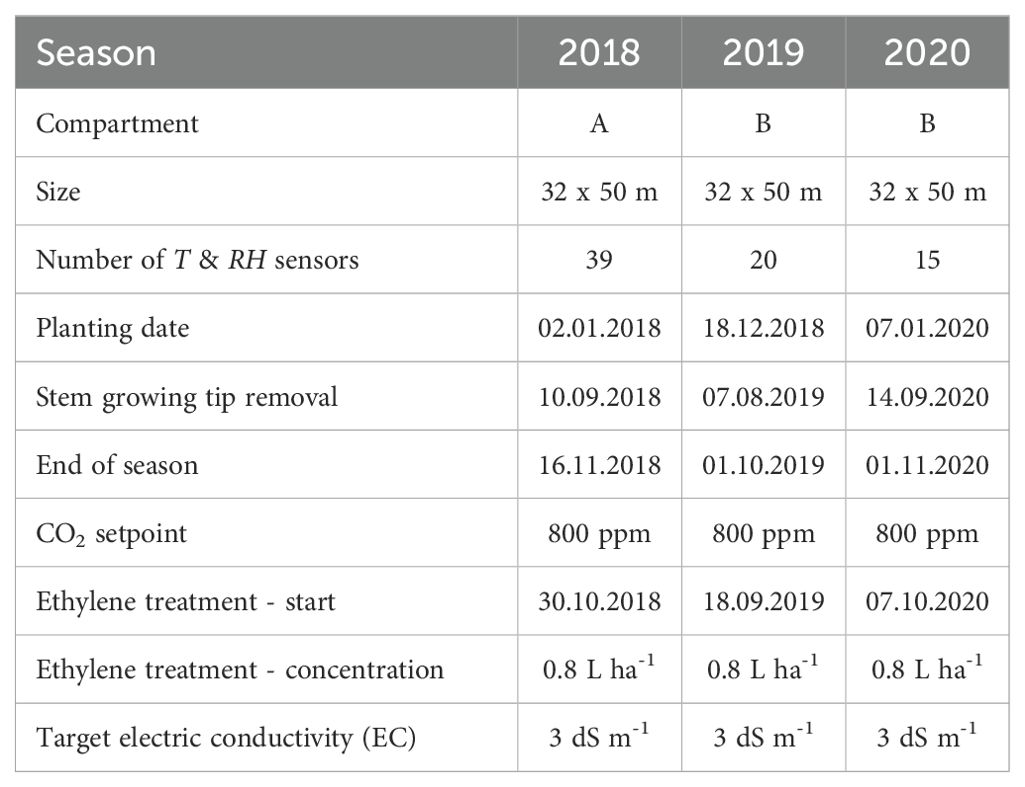
Table 1. Technical properties of the greenhouse compartments and details of the growing seasons.
2.2 Climate conditions and monitoring
General greenhouse climate was monitored by one central weather station (Electronic Measuring Box, Priva, De Lier, The Netherlands) just above the crop canopy in the middle of each compartment, logging T and RH every 5 minutes. The temperature regime from the time when fruit were present on plants was set to be 20 °C during the daytime, 16 °C from sunset until midnight and 18 °C for the rest of the night with slight variations in setpoints during the year. Roof ventilation started when the temperature reached 2 °C above the setpoint. No active cooling (other than opening roof windows) and shadowing management were present. More details about the growing conditions are presented in Table 1.
During 2018 and 2019, T and RH sensors (SHT31 Smart Gadget, Sensirion, Stäfa, Switzerland) logged values every 15 minutes (accuracy T ± 0.2 °C, RH ± 2 %). In the 2020 season, monitoring devices developed in the GROW! project (Interreg Vl-Nl1) with build-in T and RH sensors (SHT31, Sensirion, Stäfa, Switzerland) were used (Singh et al., 2020). Sensors were placed at the top of the canopy at the height of the upper leaves. During all seasons, sensors covered a large part of the greenhouse compartment area and were located in proximity to plots used for monitoring plants (Figure 1). In 2018 sensors were distributed across the compartment to determine its microclimate (Figure 1A). In 2019 (Figure 1B) and 2020 (Figure 1C) sensors were placed mostly in a priori identified microclimate zones. Two light sensors (SQ 300, Apogee Instruments, Santa Monica, USA) measuring photosynthetically active radiation (PAR) were placed at the top of the canopy, logging values every 10 minutes (Figure 1). All measured environment data are available in the accompanying repository (Salagovic et al., 2024).
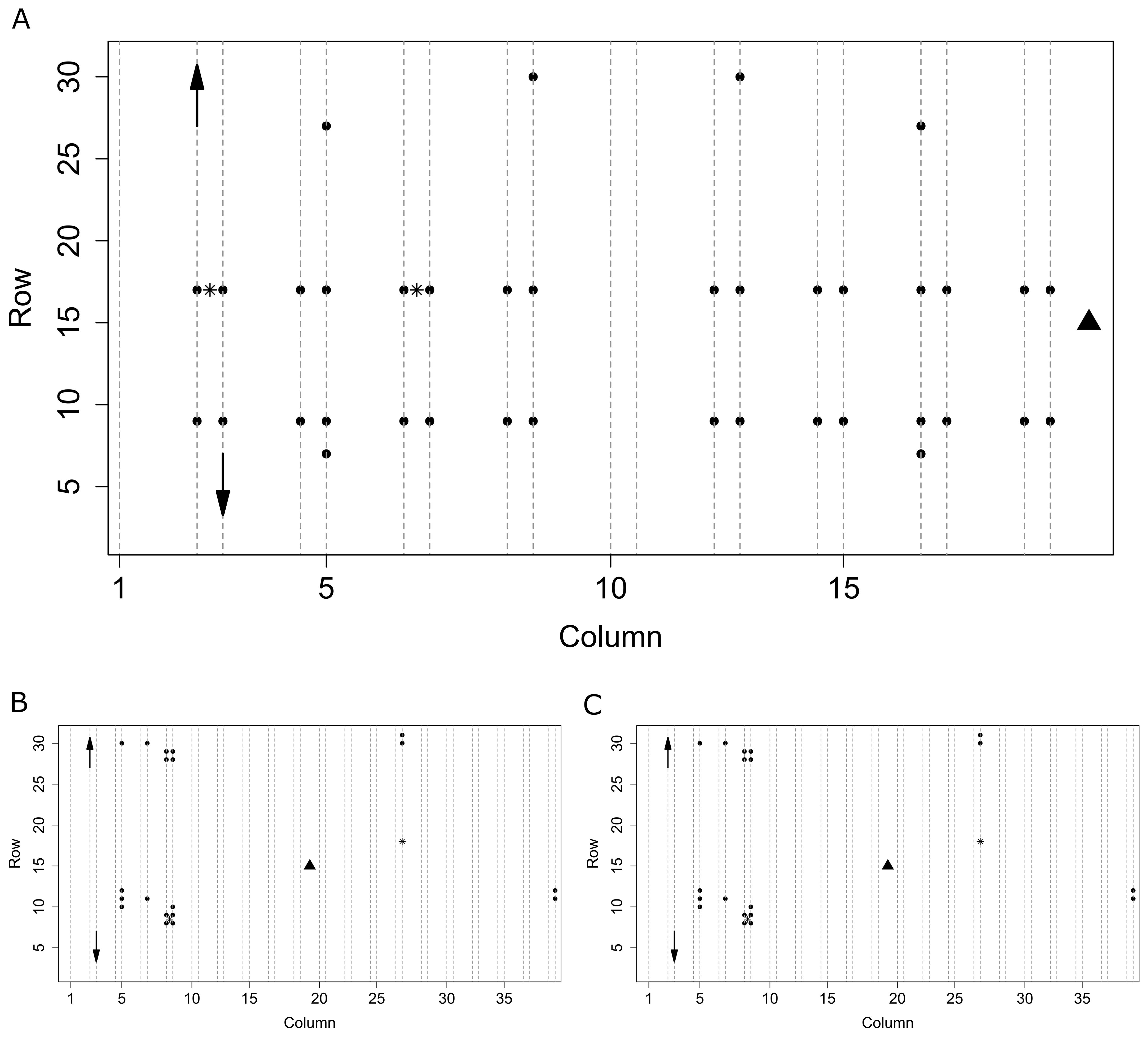
Figure 1. Spatial organisation of the sensors in the compartments of the greenhouse in seasons 2018 (A), 2019 (B), and 2020 (C). Dotted lines represent plots with plants, circles represent Sensirion T+RH sensors, the triangle is a central weather station, stars are light sensors. Arrows schematically show the direction of movement of plants (and in 2018 and 2019 also sensors) within columns of odd and even numbers moving in the same direction as for the first two shown.
Sensors were either stationary or moved along with the plants when they got bigger. For the 2018 and 2019 seasons, plants and their accompanying sensors were rehanged within the column after reaching the maximum wire height, changing their y position in directions as shown in Figure 1. Sensor movement thus resulted in a dynamic spatial grid, changing over time, but always linked to one particular plant. The maximum distance each sensor moved from its original position was approximately 7 meters, limited by maximum plant stem length at the end of a season. In the 2020 season, sensors were kept at their original position during the whole season, while plants were rehanged in a regular way.
2.3 Microclimate calculation
VPD was calculated by the Buck equation (Buck, 1981) as the difference between the water vapour pressure of saturated air (RH = 100 %) and the actual water vapour pressure, corresponding to the measured RH and T.
To obtain climate information for every position in the greenhouse, the Akima interpolation algorithm (Akima, 1978) implemented in R (R Core Team, 2013; Akima et al., 2016) was used to calculate the horizontal distribution of T and RH in 2018. The algorithm uses continuously differentiable spline interpolation working with an irregular grid of x and y coordinates on a plane with the z dimension representing climate values (T or VPD). Only values inside the area defined by the convex hull of available sensors were used to create a regular grid inside the convex hull by interpolation. In 2019 and 2020 only the recordings from individual sensor locations were used without interpolation.
The day period was defined as a period when light sensors measured values above a defined threshold of 10 µmol m-2 s-1, while the other time points were defined as the night period. To investigate the daily behaviour of microclimate evolution of a single day over 3 years in more detail, September 23rd was selected as a case study.
The use of degree-days models is widely accepted for building phenology models (Edey, 1977; Roltsch et al., 1999). Here, the growing degree days (GDD) model as described by Pathak and Stoddard (Pathak and Stoddard, 2018) was used with a base temperature of 10 °C and cutoff temperature of 30 °C, commonly used to describe tomato growth. GDD values were calculated for each day separately for up to 84 days prior to harvest (upper limit for fruit development of cv. Merlice), calculating a cumulative GDD value for each day.
2.4 Plant and tomato fruit measurements
Stem growth rate and fruit yield were monitored on a weekly basis during seasons 2018 and 2019. The stem growth rate was calculated as an increment of the previously labelled position and the top of the stem over the time between measurements. Fruit appearance rate was monitored by keeping track of the timing of the most recently appearing truss with fruit. The number of the highest truss was incremented with each new truss throughout the whole season, with the oldest truss being number 1. For yield monitoring, trusses were harvested according to industry specifications, empirically based on fruit size and colour. The fresh weight of the whole truss was measured on the day of harvest. Early in autumn, the growing tip of each plant was removed (Table 1), omitting apical stem growth and truss initiation from that moment onwards.
Fruit growth was monitored weekly during two periods in 2020 by following the growth of selected trusses from flower anthesis until red ripe fruit. Trusses were labelled at the beginning of anthesis on June 5th 2020 and August 31st 2020. Labelled trusses had, therefore, flowers in the same development stage (i.e., fully open flowers). Three trusses per microclimate zone were harvested each week. On the day of harvest, the equatorial maximum diameter and fresh weight of each fruit were measured. Dry weight was determined after drying at 70 °C until a constant weight was reached (1 week).
For quality assessment, additional trusses were harvested for a period from April 14th to October 5th 2020 according to industry specifications. Tomatoes were transported from the greenhouse to the laboratory (Flemish Centre for Postharvest Technology, Leuven, Belgium) and stored at T = 18 °C and RH = 80 %. The next day firmness, colour, weight and ethylene production were monitored. Firmness was measured with a texture analyser (TA.XT Plus, Stable Micro Systems, Godalming, UK) fitted with a 3.5 mm diameter probe attachment. Firmness was assessed by compression over a distance of 2 mm at a speed of 2 mm s-1 at two sides of the equator of the fruit. Colour was measured with a handheld spectrophotometer (CM-2500d, Minolta, Kontich, Belgium) twice on opposite sides on the equator of the fruit. Colour was quantified by measurements of hue angle (°) and lightness (on a scale of 0-100). Ethylene measurements were done with a Compact GC (MEB 07061594, Interscience, Louvain-La-Neuve, Belgium) after fruit weight was recorded. Individual tomatoes were placed in glass jars for 2 hours at 18 °C, allowing ethylene to accumulate in the headspace. Soluble solid content was measured by extracting a few droplets of tomato juice and placing it on a digital refractometer (Atago PR-101 alfa, Analis, Gent, Belgium).
A principal component analysis (PCA) was performed on quality data. Principal components were retained on the basis of eigenvalues greater than 1. The PLS_toolbox (version 8.9.1, Eigenvector, Manson, USA) in Matlab (Matlab R2021b, The Math-Works, Natick, USA) was used for this analysis.
2.5 Statistical analyses
To test if tomatoes from different conditions (e.g., different climate conditions, different pruning strategies) were having different properties (e.g., fresh weight), analysis of variance (ANOVA) with a level of significance α = 0.05 was used. Data were assumed to be independent. Prior to ANOVA, homoscedasticity was tested by Levene’s test (Levene, 1960) and normality by the Shapiro-Wilk test (Shapiro and Wilk, 1965).
To assess the effect of microclimate on tomato growth, we used separate datasets of temperature history accumulated by a plant (from GDD) through a growing period and average daily VPD as independent variables. The dependent variables were truss weight and stem growth rate. For independent variables, we used a list of n values representing n days prior to measurement. We tested different values of n ranging from 7 to 84 days for the highest explained variance across all datasets. For example with GDD, the lowest used value, n = 7, implies a dataset of 7 GDDs of the last 7 d before the harvest day as 7 predictor variables (GDD of day 1 before harvest, GDD of day 2 before harvest, etc.). The upper limit of n = 84 was selected based on the time from anthesis until harvest for this cultivar, which ranges between 10 to 12 weeks. The number of predictors (n) could, therefore, exceed the number of observations (harvested trusses for the selected period). Moreover, multicollinearity is naturally present in the dataset, as is generally the case of highly correlated predictor variables (Alin, 2010), as daily temperatures tend to be highly correlated to the temperatures of the previous day. The determinant |X’X’|-1 <10-150 was close to zero for predictor variable set X and therefore confirms multicollinearity in the dataset (Farrar and Glauber, 1967). Linear ridge regression was used to determine a relationship between local microclimate and tomato growth as it takes multicollinearity and datasets with a higher number of observations into account (Hoerl and Kennard, 1970; Marquardt and Snee, 1975).
To reach more uniform effects of other variables (e.g., plant age) and limit seasonal effects of climate, measurements were also analysed for a shorter time period, not just over the whole season. To minimise the effect of other known conditions (e.g., sunny vs shaded canopy side) data were processed to have an equal representation of each of these known factors.
3 Results
3.1 Average greenhouse climate conditions show seasonality
We observed a seasonal trend for temperature and VPD data for each year (Figure 2). The average monthly temperature increased from spring months (e.g., January 2020: 16.8 ± 2.7 °C), reaching a maximum in summer (August 2020: 22.4 ± 4.2 °C) and decreasing in autumn (October 2020: 20.0 ± 2.1 °C) (Figure 2A). Temperature variation over time was the highest in summer, and the lowest in the colder months of winter and autumn. Seasonal trends between observed years were similar with only a few periods each year with climate varying from other years.
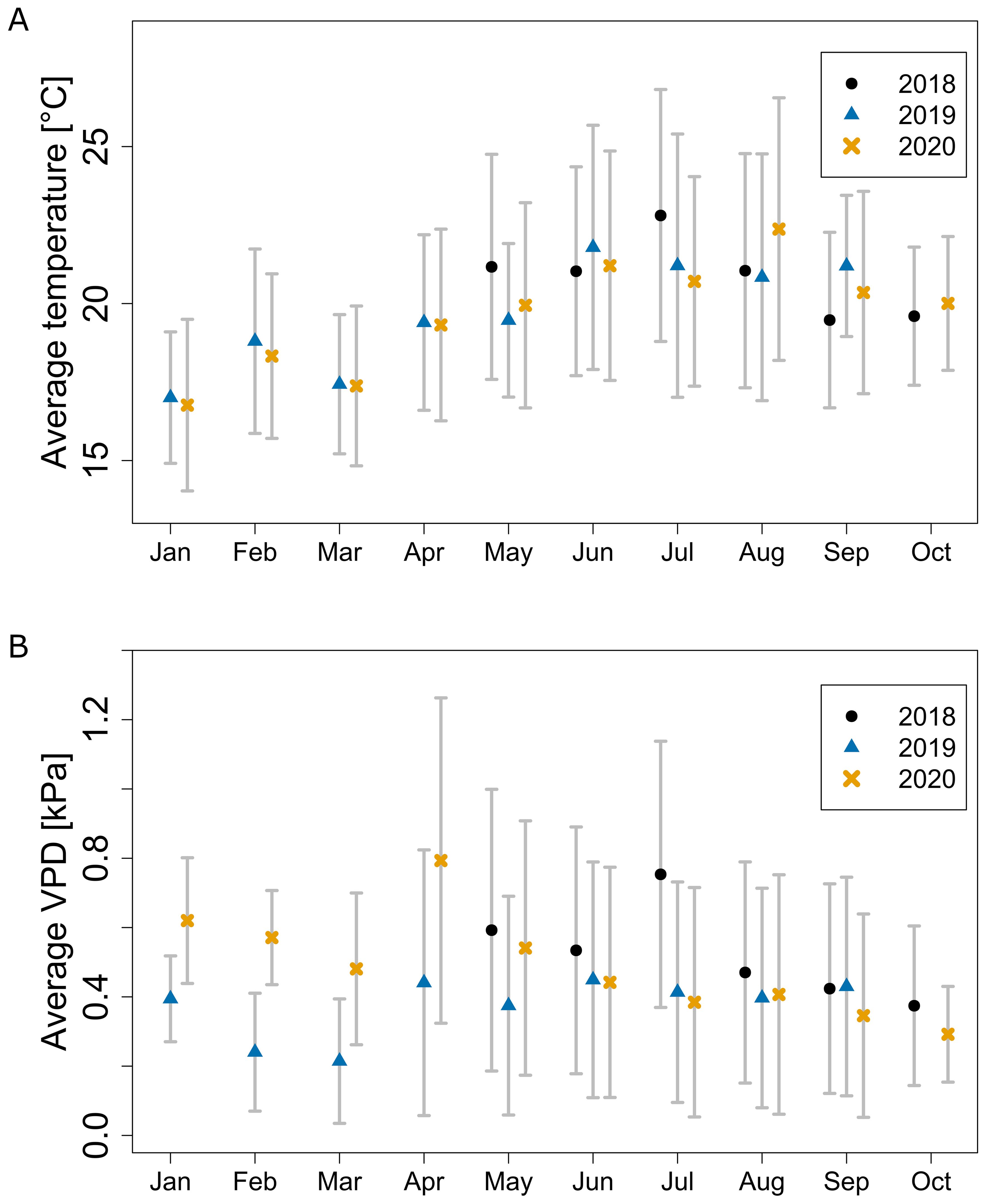
Figure 2. Average monthly greenhouse temperature (A) and VPD (B) throughout the seasons measured by the central weather station. Error bars show standard deviation over time.
The average monthly VPD followed a different trend compared to temperature: a slow drop from January to March, a sharp increase to peak in April, followed by a slow decrease until the end of the season (Figure 2B). During the period from June to September, the average VPD across all seasons equalled 0.47 ± 0.34 kPa. The lower VPD in February and March was, except for lower temperature, caused by a higher relative humidity. The RH in 2019 and 2020 for that period was respectively on average 6.1 and 5.3 percentage points higher than for the rest of the year. VPD variation over time was following a similar trend as temperature with high variance during the summer months, but unlike temperature, being the highest in April and May (Figure 2B). Results for both temperature and VPD showed seasonal effects matching the outside climate and revealed possible sub-optimal growth conditions for some periods, especially for VPD (Shamshiri et al., 2018).
3.2 Identification of microclimate zones across the greenhouse
A sensor grid within the greenhouse revealed the existence of a local microclimate throughout all seasons. Variations between different positions were present in all months (Figure 3). In 2019, the highest daily differences oscillated around 1.5 °C, with peak differences in August increasing up to 7.17 °C (Figure 3B). Extremes with higher average local temperatures were reached only for isolated days, probably caused by direct solar heat radiation. Microclimate variation was not only present in summer but also during colder months of spring and autumn, presumably caused by non-uniform heating, as the main determining factor that controls the inside climate during these periods. Light measurements at the top of the canopy did not show significant differences in weekly average irradiation between the two monitored locations.
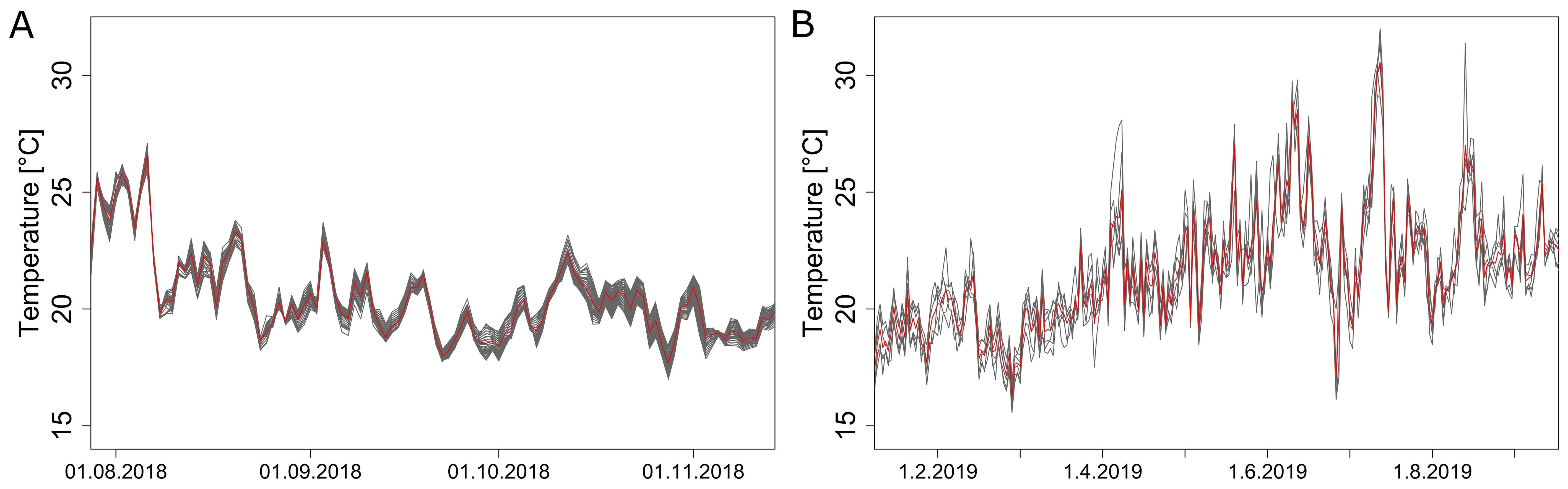
Figure 3. Differences in the average daily temperatures measured by the sensor grid at different positions in 2018 (A) and 2019 (B). The red line represents the average temperature over all positions, black lines are temperatures at different positions. Displayed are daily averages for all positions inside the convex hull during season 2018 (A) and for all sensors available in season 2019 (B).
Seasonal and daily changes were not only affecting the mean temperature and vapour pressure deficit, but also their spatial distribution profiles. The observed microclimate was, therefore, not static but was changing over time. During the 2018 season, the difference between the warmest and coldest positions in the greenhouse during one day was largest in warmer summer months (up to 4.8 °C) and smallest in autumn (down to 0.8 °C). Similarly, in 2019 the highest differences were recorded in summer (up to 5.5 °C) and the lowest in autumn (down to 0.3 °C). The largest average monthly temperature differences were observed during the day (Figure 4) and not during the night. The temperature difference between the warmest and coldest recorded positions was lower during colder months at the beginning and the end of the year (Figure 4). The opposite trend was present for night temperature differences.
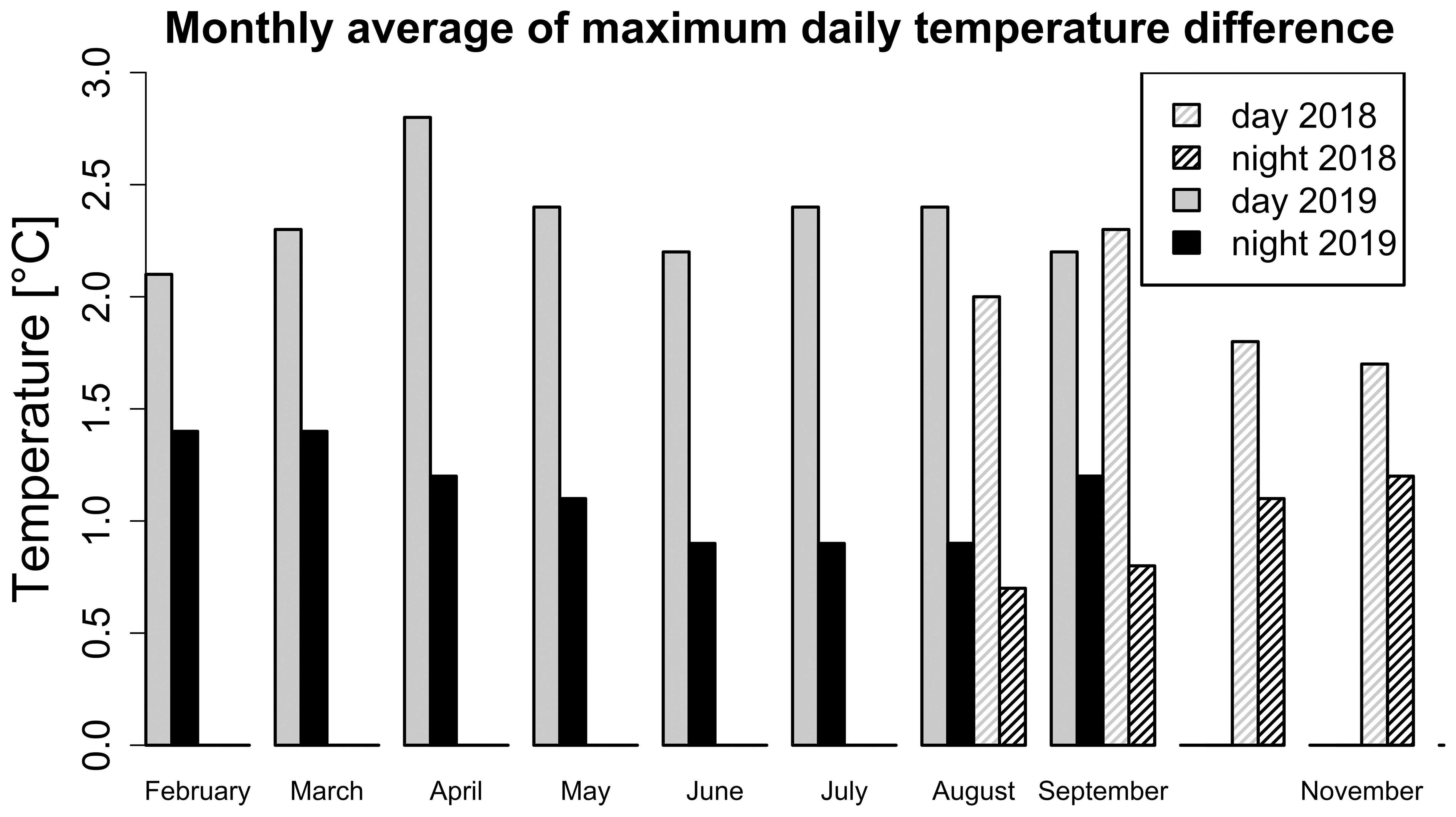
Figure 4. Monthly average of the maximum average daily temperature variation for the day (black) and the night (grey) in seasons 2018 (pattern) and 2019 (filled). The maximum average daily temperature variation was calculated as a difference of maximum and minimum average daily temperature from all sensors available. November period ends on 17.11.2018.
To localise regions with high and low T and VPD variability, the microclimate of the whole greenhouse compartment area was analysed using heatmaps (Figure 5). In August 2018 (Figure 5A), the highest difference in average monthly temperatures from all positions was 1.1 °C. The temperature distribution pattern shows most of the variation during the day (Supplementary Figure S1A) with almost uniform night temperatures (Supplementary Figure S1C). The VPD, shows a similar pattern as the temperature heatmaps, with deviations caused by different RH profiles. In August 2018, the average monthly spatial difference in VPD was between 0.6 to 0.8 kPa (Figure 5B). Spatial VPD differences during that month were more pronounced during the day than during the night (Supplementary Figures S1E, G). The main source of greenhouse climate variation in summer was the outside weather condition. During warmer nights, heating was less needed.
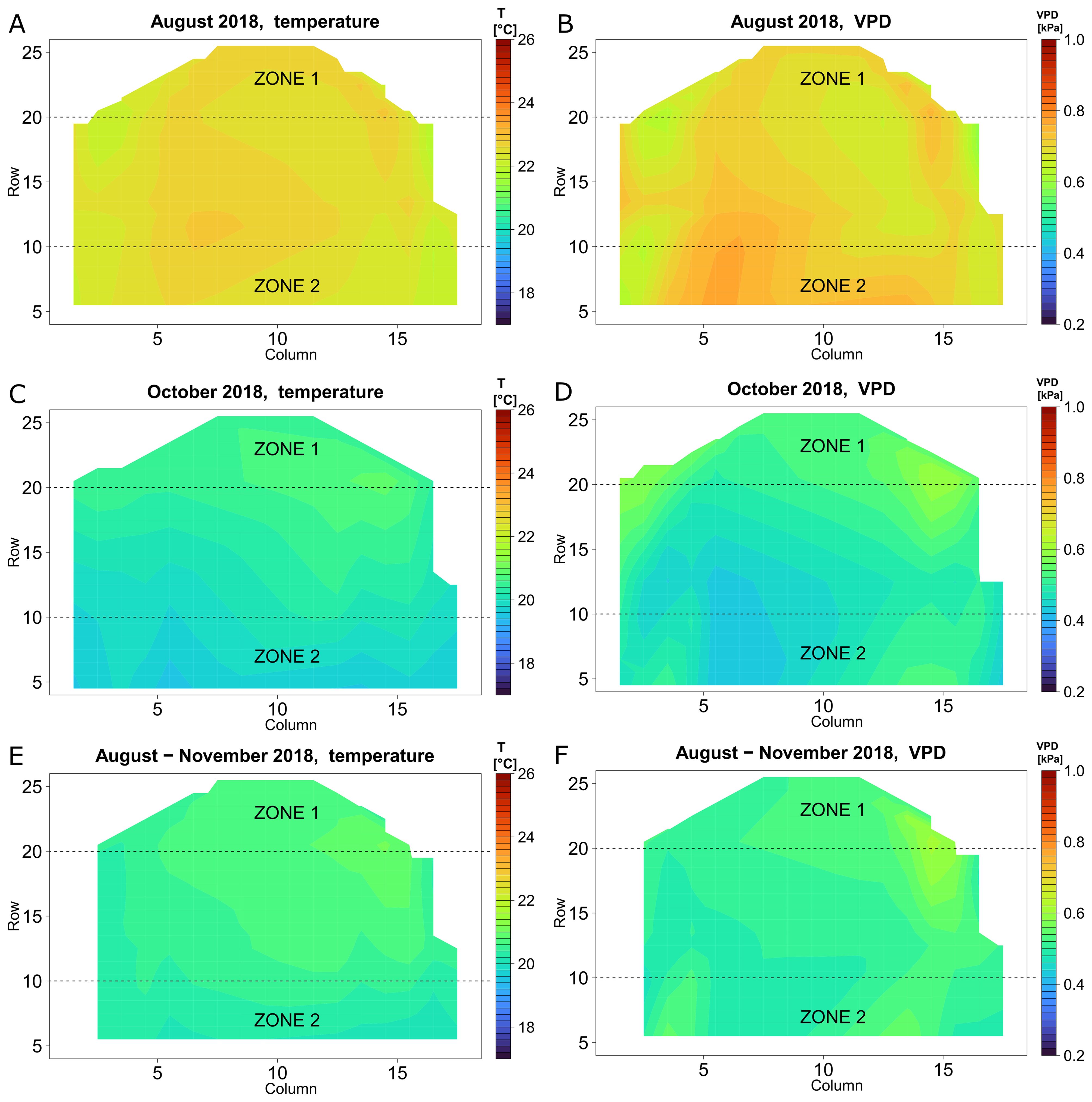
Figure 5. Heat maps of the microclimate inside the greenhouse in 2018, whole day. Temperature (A, C, E) and VPD (B, D, F) in August (A, B), October (C, D) and the period of August-November (E, F).
A different spatial microclimate gradient was observed, especially towards the end of the season. In October 2018, a linear gradient in temperature was present, increasing with the row number (Figure 5C), with a maximal difference of 1.4 °C. This higher difference in comparison to the month of August was caused by the greater differences in the night microclimate (Supplementary Figure S1D) in combination with a similar temperature distribution pattern that was present during the day (Supplementary Figure S1B). The VPD gradient increased with row number (Figure 5D) which corresponds to the temperature microclimate distribution. This spatial trend in T and VPD was also present when the microclimate data were analysed for the whole period from August until November (Figures 5E, F). In conclusion, we noticed that there mainly was a temperature and VPD gradient present along the rows, but less so along the columns. Based on these gradients, we defined two zones: zone 1 (in the upper third region, rows 21 – 30) was the warmer and drier zone, while zone 2 (in the lower third region, rows 1 – 10) was the cooler and more moist zone. Next, we analysed the microclimate effect of these two zones in more detail, for the seasons 2018 – 2020.
3.3 Diurnal microclimate differences between two zones
In 2018, zone 1 was on average warmer than zone 2, especially in autumn when the average daily temperature was below 23 °C (Figure 6A, Supplementary Figure S2A). The difference between zones steadily oscillated around 1 °C from late September. In 2019, the temperature difference was highest from January to March when the daily average temperature was rarely above 20 °C (Figure 6C, Supplementary Figure S2C). A similar trend was present in 2020 (Figure 6E). In general, during summer periods with higher temperatures, spatial temperature differences were fluctuating around zero with a few extremes, while in colder months, spatial variability between the two zones was more pronounced. VPD varied more between the zones on days with a higher maximal VPD, both in 2018 (Figure 6B, Supplementary Figure S2B) and 2019 (Figure 6D, Supplementary Figure S2D). During colder months of all years, there was an average difference of 0.1 kPa between zone 1 and 2, while other periods oscillated around 0 kPa (Figures 6B, D, F). Both temperature and VPD showed a similar spatial variability throughout the season.
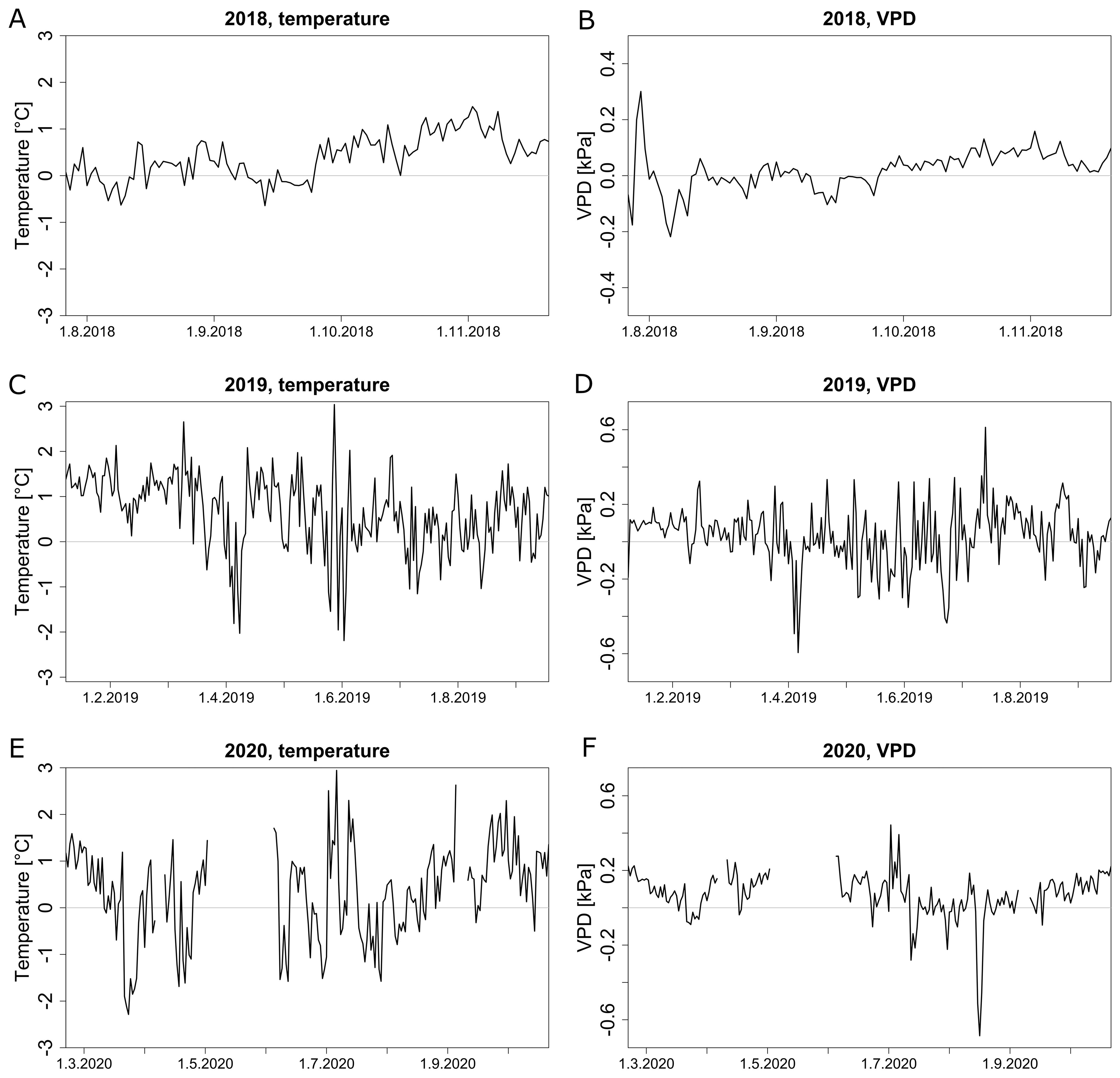
Figure 6. Comparison of temperature and VPD profiles between different zones (zone 1 and zone 2 identified in Figure 5). Average daily temperature difference (A, C, E) and VPD difference (B, D, F) between zones 1 and 2 in 2018 (A, B), 2019 (C, D) and 2020 (E, F). Missing data points are due to sensor failures or dead batteries.
For a selected day, September 23rd, different diurnal profiles were observed between the years for both temperature and VPD (Figure 7). The overall climate profiles and microclimate differed from year to year based on the actual outside weather and the corresponding greenhouse management practices. An unusually warm evening in 2020 (Figures 7E, F) was responsible for the highest microclimate difference (up to 2 °C and 0.2 kPa) between the two zones, and showed an uncommon climate evolution throughout the day versus other years. Microclimate differences between zones during the night were relatively stable, while microclimate differences during the day showed greater variation between the zones.
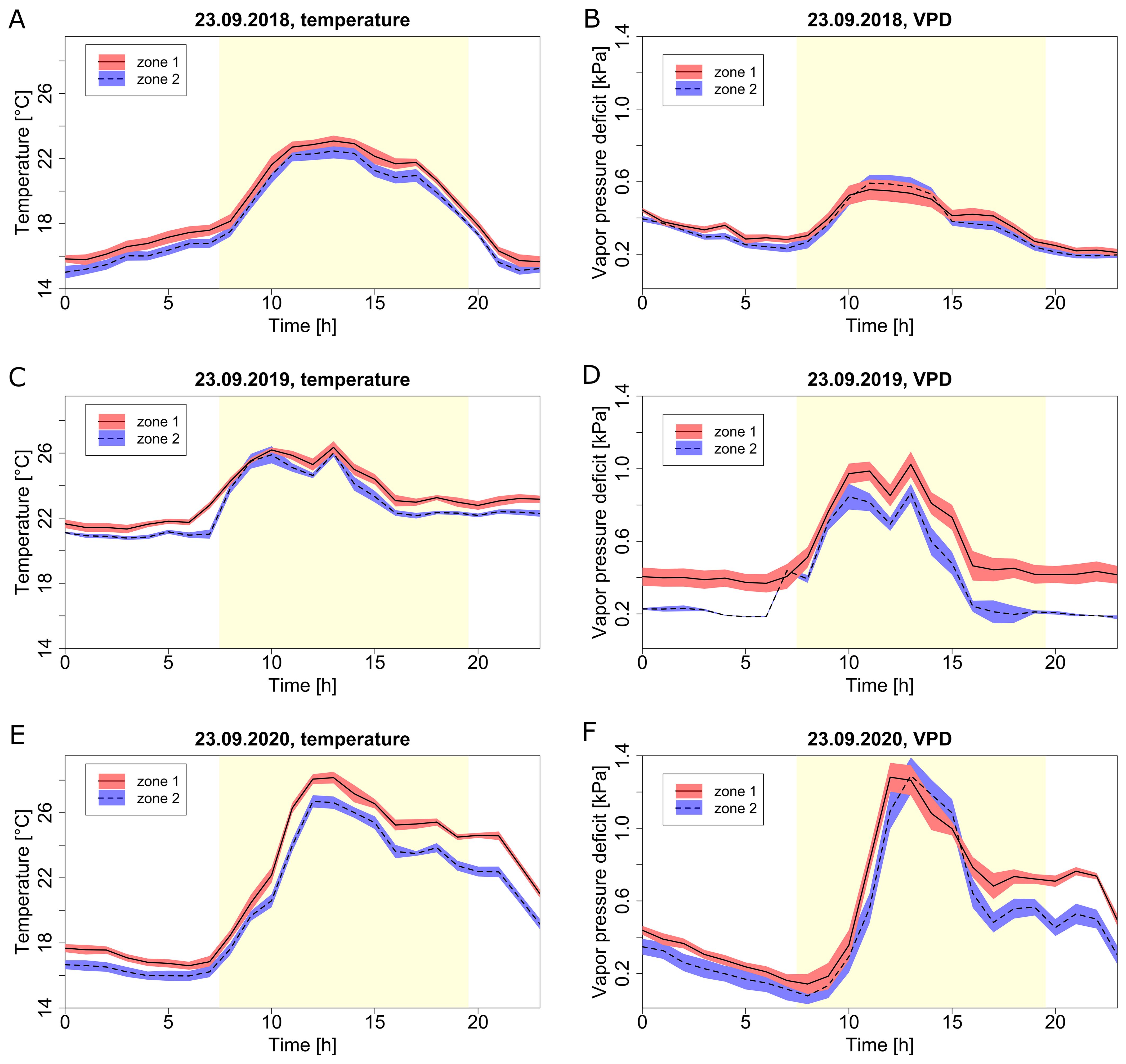
Figure 7. Diurnal climate profiles at different zones (zone 1, red; zone 2, blue) for the selected day of September 23rd during three seasons. Temperature (A, C, E) and VPD (B, D, F) for season 2018 (A, B), season 2019 (C, D) and season 2020 (E, F). Lines represent the hourly average, the red and blue shaded areas represent confidence intervals. The day period is marked by the yellow area, while the night is the white area.
3.4 The local microclimate influences plant growth and fruit yield
To study the effect of the local microclimate on fruit production, we analysed crop growth and fruit yield in the two zones. However, we first analysed the effect of the different leaf pruning strategies using ANOVA, but did not discover any significant difference for stem growth and fruit yield between the different pruning strategies (data not shown). Therefore, we ignored the pruning variable and pooled the data for the subsequent microclimate analysis.
Plant growth and truss weight were significantly affected by the microclimate conditions. Both in 2018 (Figure 8A) and 2019 (Figure 8B), the truss weight was on average higher in zone 1 compared to zone 2. However, this difference was only significant in May and September 2019 (Figure 8B). Plant growth variables such as stem growth rate and highest truss number on a plant were showing the same trend in 2019, with plants growing faster in zone 1. The differences between the zones in 2019 were significant in May, but not in July (Figures 8C, D). In general, a warmer microclimate (zone 1) leads to a higher stem and plant growth rate, which leads to a higher fruit truss weight, during certain periods of the year.
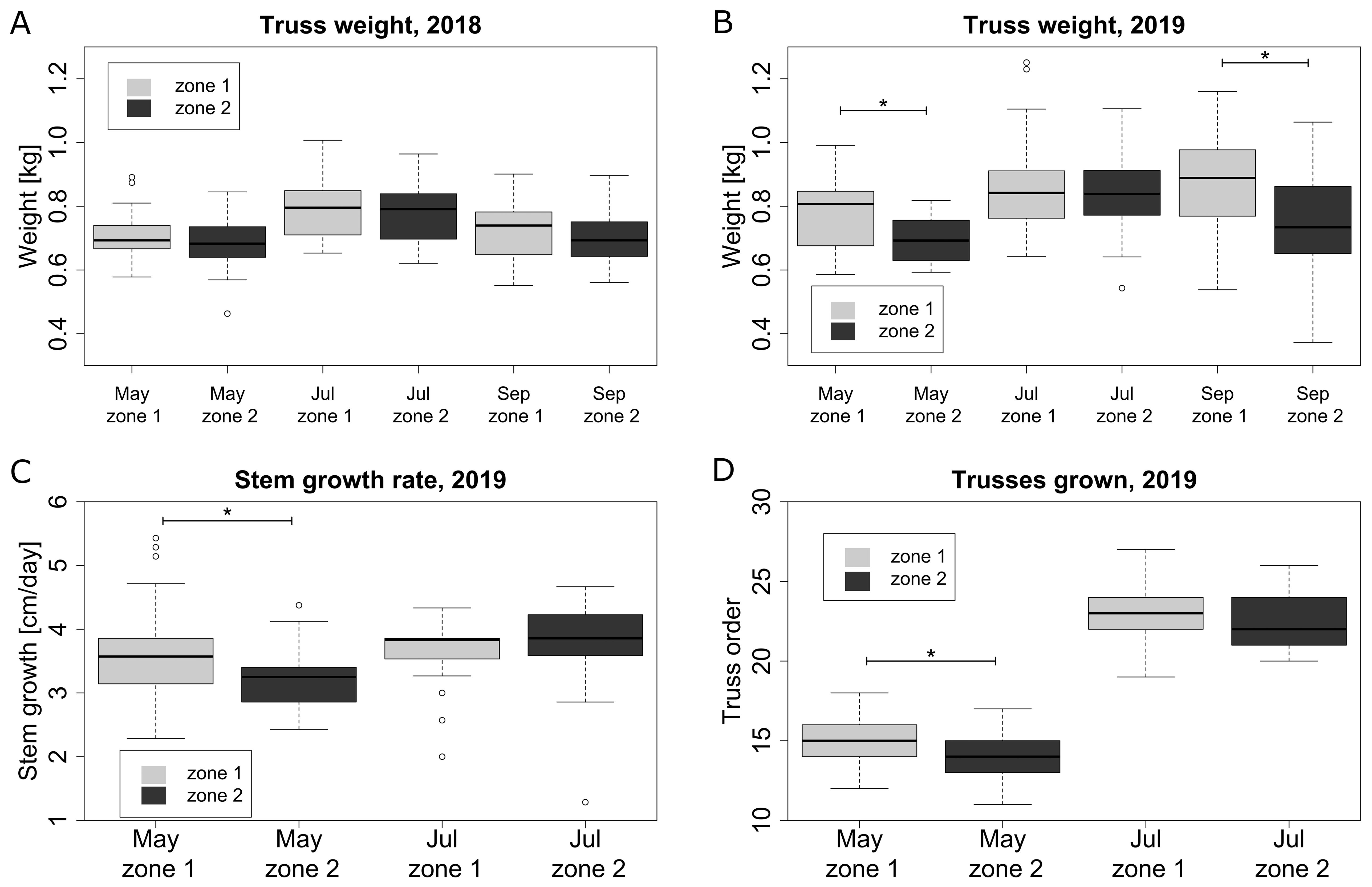
Figure 8. Plant growth and fruit attributes for two microclimate zones for selected representative months: truss weight in 2018 (A) and 2019 (B), stem growth per day in 2019 (C) and the number of trusses grown on plant including trusses currently on plant in 2019 (D). Columns marked with * are significantly different within the same month.
3.5 Tomato quality is not affected by microclimate
We investigated the hypothesis that tomato fruit quality would be affected by the microclimate in a similar way as was shown for plant growth and truss weight (Figure 8). The variation in quality between tomatoes was analysed by PCA. Most of the variability in quality was caused by variability in colour, as hue and lightness were closest related to PC1 (46.28 %) (Supplementary Figure S3A). Differences in ethylene production and fruit weight were more closely associated with variability caught in PC2 (23.41 %). Overlapping point clouds indicate no differences between fruit quality and their position in the truss (Supplementary Figure S3B). The microclimate did not have a significant effect on fruit quality on day 1 after harvest, as the point clouds also intersect. Likewise, this was the case for tomatoes harvested in different months (Supplementary Figure S3C), although tomatoes harvested in June tended to weigh slightly more versus those harvested in April or October. The lack of any detectable microclimate effect on fruit quality is likely caused by the large heterogeneity of harvested fruit, as they are manually picked based on a visual inspection of colour.
3.6 The local microclimate conditions predict differences in tomato plant and fruit development
To expand our analysis beyond the predefined microclimate zones and to evaluate the effect of local climate conditions on plant growth and fruit yield, we used a ridge regression model with local microclimate dataset. Interestingly, the ridge regression model could explain the greatest variance across all datasets at a time period of 70 days of fruit development (analysis not shown). This period approximates the time from fruit anthesis until full ripening (although this can vary throughout the season).
Comparing measurements and predictions of the model for different climate datasets on the input (e.g., collected from one central weather station vs from local sensors) can reveal which one explains the most of the observed differences in dependent variables (e.g., stem growth rate). By using only data from the central weather station we were able to explain 79.8 % of the variance for average daily stem growth in 2019 (Figure 9C, Table 2). When incorporating local microclimate data, the explained variance increased to 84.9 % in 2019 (Figure 9D, Table 2). The dataset from 2018, covering a shorter growing period, had an explained variance of 79.1 % based on the central weather station (Figure 9A, Table 2) and 93.3 % when using microclimate sensor data (Figure 9B, Table 2).
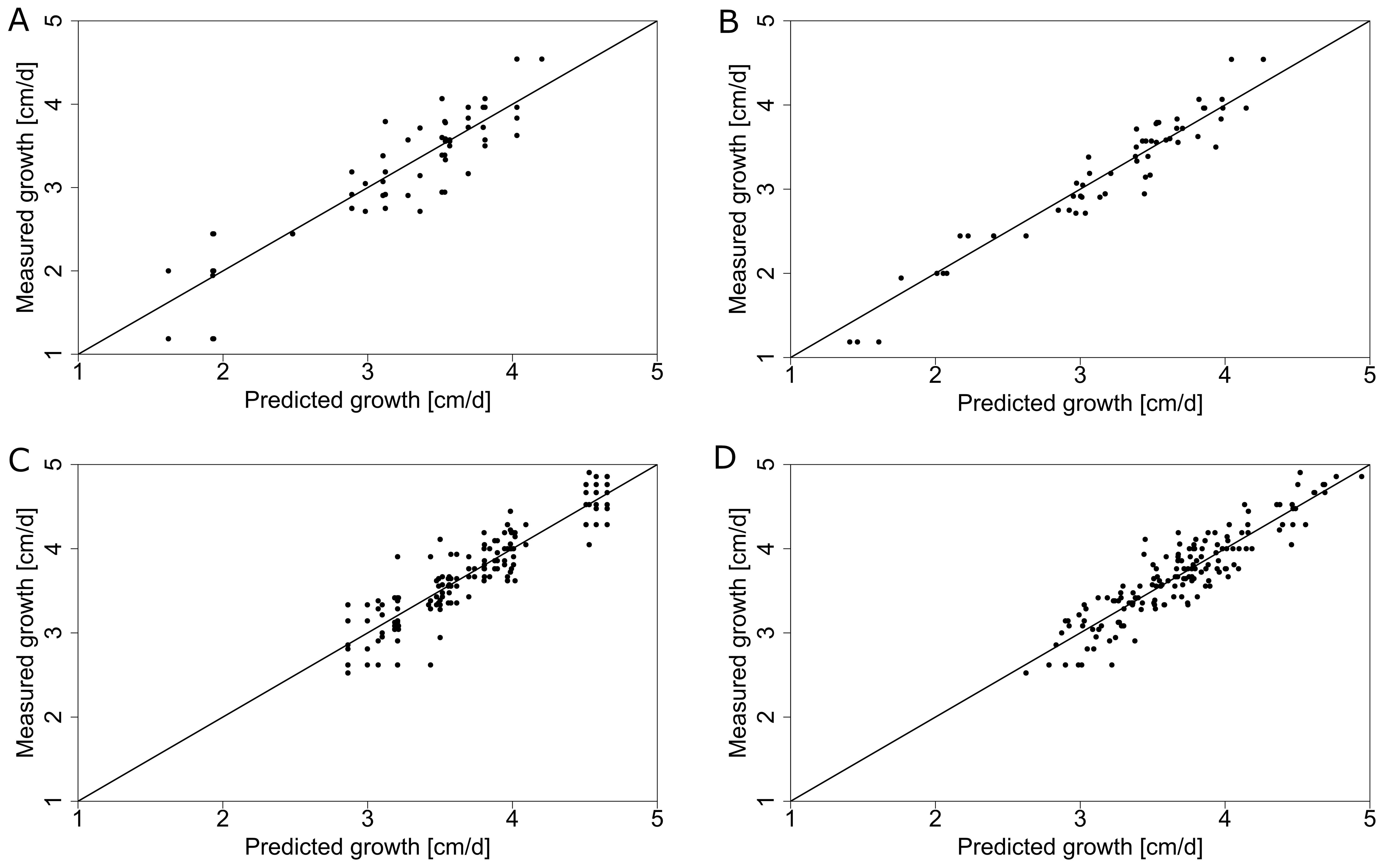
Figure 9. Daily stem growth (measured vs predicted using the ridge regression model) using global GDD based on the central weather station (A, C) and different position-specific GDD that captures the local microclimate (B, D) for 2018 (A, B) and 2019 (C, D). The solid line represents the ideal theoretical fit and the dots represent individual measurements.
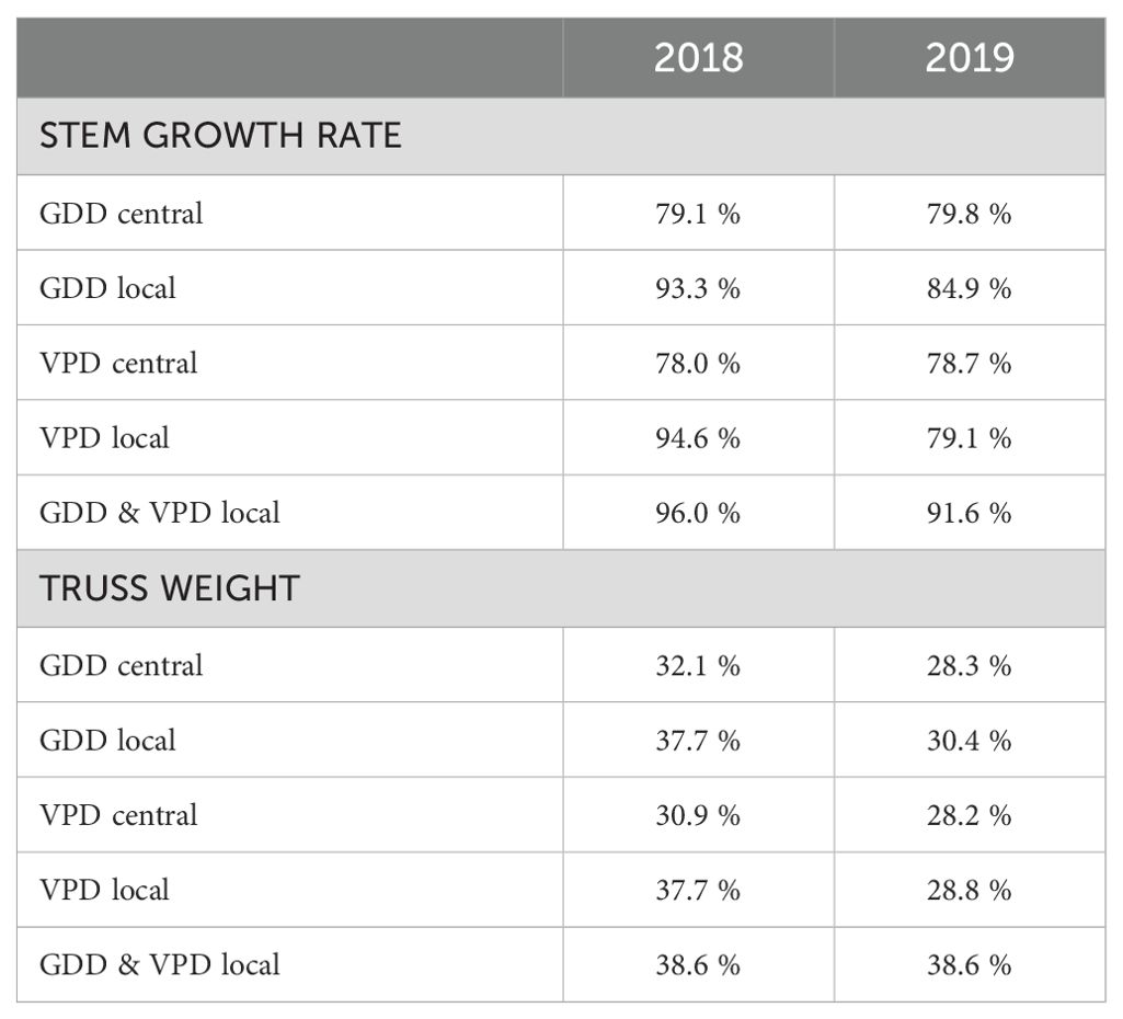
Table 2. Explained variances of the ridge regression model’s predictions for 2018 and 2019 seasons using different inputs (GDD and VPD, from weather station – central or using microclimate – local) with dependent variables being separately stem growth rate and truss weight.
Applying the same ridge regression model approach to truss weight from 2019, we were able to increase the explained variance from 28.3 % when using one GDD value per harvest date from the central weather station to 30.4 % when using local microclimate data (Figure 10, Table 2). In the smaller dataset of 2018, we obtained an explained variance of 32.1 % when using GDD from the central weather station and 37.7 % when using microclimate. For most of the harvest dates, the mean of the predicted truss weight is close to the ideal model fit with evenly distributed points around the mean when using GDD from the central weather station (Figure 10A). This means that despite a relatively low explained variance, the prediction for the average truss weight of each harvest date corresponded to the measurements (Figure 10A). Results using local microclimate GDD data show a slightly better fit (Figure 10B), as quantified in Table 2. Using local microclimate data increased the explained variance for both stem growth rate and truss weight in all seasons.
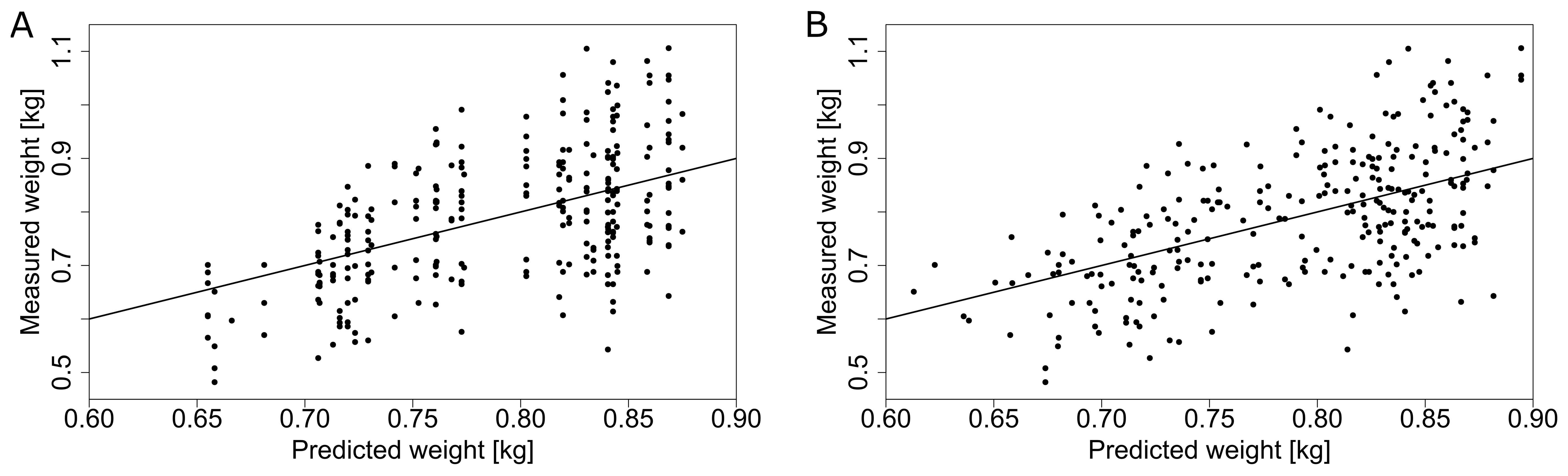
Figure 10. Prediction of truss weight (with 5 tomatoes per truss) based on the GDD obtained from the central weather station (A) and GDD from the local microclimate sensors (B) for the dataset in 2019. The solid line represents an ideal theoretical fit and the dots represent individual measurements.
The ridge model using for input data the VPD microclimate as a predictive variable outperformed the model with GDD microclimate on input only for the prediction of stem growth rate in 2018 (Table 2). In all other scenarios, the explained variance was higher with GDD data for input. For all scenarios, the best results were achieved by a model that uses both GDD and VPD as input data (Table 2). Using local microclimate data compared to using data obtained from the central weather station, the explained variance for truss weight in 2019 rather increased for all months (Table 3). The exception was the prediction for August, where the explained variance increased only by 0.1 percentage points.
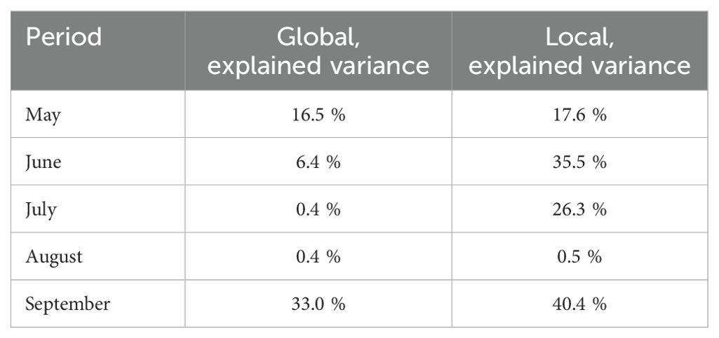
Table 3. Explained variances for truss weight of the ridge regression model’s outputs for different months of season 2019 when using one central sensor (global) and when using microclimate data (local).
3.7 Long-term effects of the microclimate on growth rate
To unravel the effect of microclimate on tomato fruit growth rate, two experiments were conducted during which fruit growth was followed up weekly, by labelling trusses at anthesis. Trusses from the warmer zone 1 showed a higher fruit growth rate versus the cooler zone 2 for both experiments (Figure 11). Fruit fresh weight for both zones had at a similar initial value, but fruit from zone 1 grew faster than the ones in zone 2. The final average weight was not significantly different between both microclimate zones. The analysis indicated that the main effect of the microclimate differences was on fruit growth rate rather than final fruit mass. The microclimate effect on fruit growth rate was present in both a warmer (summer) and a colder (autumn) period. In the period from June to August, the GDD difference between both zones was 14 °C days, while for the period from September to November it was 81 °C days.
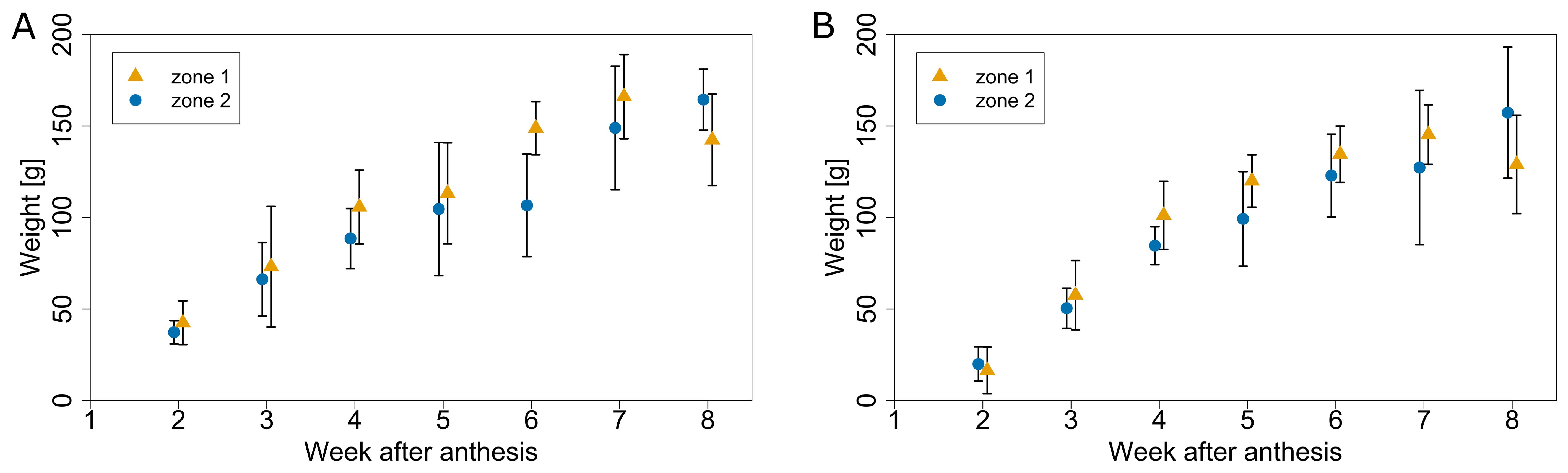
Figure 11. Average fruit weight for different microclimate zones (warmer zone 1 in yellow and a cooler zone 2 in blue) at different times after anthesis for the season 2020. Fruit growth profiles were obtained in early summer (A) anthesis on 5.6.2020) and during autumn (B) anthesis on 31.8.2020). Error bars represent standard deviation of samples collected for each date.
Truss growth rate can affect the total number of trusses harvested per plant per year, especially when correlated to the truss appearance rate. In 2018, the average amount of trusses harvested per plant was 29.83 and 29.04 for zones 1 and 2, respectively. In 2019, a slightly shorter season, the number of trusses harvested were 27.69 and 25.56 for zones 1 and 2, respectively. Long-term microclimate effects accumulated throughout the season resulted on average in a difference of 8 % for the number of trusses harvested per plant between the two zones.
4 Discussion
4.1 Temperature and VPD conditions are often suboptimal in a commercial greenhouse
The environmental conditions of the greenhouse changed dynamically throughout the season (Figure 2) but also during individual days (Figure 7). The temperature during three consecutive seasons was mostly within the recommended optimal range of 15 °C to 30 °C [27], with only a few daily average temperatures above the upper limit (Figures 2A, 3). Temperature variation between days was greatest in summer (Figures 2A, 3) when the effect of warm weather could not be compensated for by the greenhouse regulatory system other than opening windows. Unlike heating, which uses relatively well-established technology, greenhouse cooling still presents challenges (Kutta and Hubbart, 2014; Sethi and Sharma, 2007). Temperature variation between days during colder months was less pronounced because the outside temperature was often below the lower temperature setpoint set by the greenhouse management system. In this case, the average greenhouse temperature was maintained relatively stable by the heating system, with little ventilation from outside.
The vapour pressure deficit was for most of the months of all three seasons at the lower optimal boundary of 0.3-0.4 kPa (Figure 2B). When using T and RH data measured at plant-level (top of the canopy), VPD was most of the time within the recommended optimal range (Supplementary Figure S2) (Shamshiri et al., 2018). Still, these values were more often deviating from the optimum range in comparison to the temperature. Even though opinions on optimal conditions vary, the optimal VPD values with little or no effect on plant growth and physiology can be considered between 0.2 kPa and 1.3 kPa (Grange and Hand, 1987; Picken, 1984; Shamshiri et al., 2018). For a few days the daily VPD reached values outside of this range. A more precise hourly dataset for specific days showed that suboptimal VPD levels are more frequent, especially during the night (Figure 7). On some days, plants could even experience VPD fluctuation from too low (below 0.2 kPa) to too high (above 1.3 kPa) suboptimal values (Figure 7D). By simply measuring/recording the average climate information throughout a day (e.g., the daily average), a large part of crucial climate variation information is lost. For example, the average daily VPD of September 23rd 2019 and September 23rd 2020 of zone 1 was 0.55 kPa and 0.58 kPa respectively, but their daily profiles differ drastically up to 0.6 kPa for certain hours (Figures 7D, G). The VPD has a direct effect on transpiration and plant growth and has recently been used more often to control the greenhouse environment (Inoue and Yamori, 2021; Lu et al., 2015; Shamshiri et al., 2018). However, systems that only use stable setpoints of relative air humidity for defined periods of the day, still prevail in commercial greenhouses. Combined with greenhouse climate regulation driven by heating and opening windows, substantial suboptimal levels of VPD are present throughout many periods of the growing season.
4.2 A local microclimate is present during all seasons
We documented the presence of horizontal microclimate variation in a tomato greenhouse over the course of three subsequent years. The maximum daily difference between the two zones was 3 °C in summer, while in colder months the difference oscillated around 1 °C (Figure 6). Similar results were obtained by Ferentinos et al. (2017) with the highest heterogeneity of daily averages during summer days (up to 3.3 °C), with nights and winter periods having much lower maximum temperature variation (around 1 °C). However, these results were obtained from trials without any crop present in the greenhouse. Ogunlowo et al. (2021) found horizontal temperature differences of 1.03 °C between the central location and the sides of a multi-span greenhouse with strawberries. Balendonck et al. (2014) identified a difference of 1.2 °C on average for a short-term experiment with tomatoes. This shows that the magnitude of horizontal microclimate difference that we observed in our study is in the same range of what was reported in the past. While there exist recommended intervals of T, RH and VPD for tomato growth (Shamshiri et al., 2018), there is no agreement on acceptable horizontal differences (Balendonck et al., 2010). A common practice to avoid suboptimal climate conditions in any part of a greenhouse is using wider setpoint margins for climate control (Balendonck et al., 2014).
Our sensor network was able to observe a systematic long-term difference in the local microclimate within a greenhouse compartment over 3 years (Figure 5E). We recorded a warmer zone (zone 1) and a cooler zone (zone 2) (Figures 5, 6) (Balendonck et al., 2010). calls this type of microclimate difference static, caused by the greenhouse design and its climate regulation system. In our case, the observed differences were most likely caused by the layout of the compartment and the conditions of adjacent compartments. The colder zone 2 faced a hall passage a few meters wide with a concrete floor. This unheated thermal mass could evoke a local cooling effect on the nearby plants. The warmer zone 1 was at the outer end of the plant rows, nearby a slightly warmer compartment (for bell pepper production). There was no deterministic variation in temperature in the other horizontal dimension of the compartment, which confers with the above. On top of the observed static microclimate, a dynamic component of microclimate was also present throughout all seasons (Figures 3, 4) caused by other factors changing in time such as outside climate or plant-climate interaction (Su and Xu, 2017). No greenhouse compartment is completely homogenous in its design, crop and boundary conditions, a microclimate is thus expected to be present across the horticulture production.
Explaining differences in VPD is more complicated, as this variable is more affected by the dynamics of plant transpiration, humidification, ventilation, and weather conditions on specific days. The VPD distribution was correlated to temperature (e.g., Figures 6A, B). However, according to our heat maps of 2018 and T and RH profiles of the two different microclimate zones (Figures 5, 6), VPD seemed to vary from temperature microclimate distribution, especially during warmer months. It would require a more detailed analysis to better understand the variability of the VPD. Computational flow dynamics (CFD) models are designed to obtain spatial climate distribution in a defined mesh over time. Predictions of airflow and T and RH distribution in 3D space are inherent in CFD methods and can solve the problem of microclimate identification (Alvarez-Sánchez et al., 2014; De la Torre-Gea et al., 2011; Guzmán et al., 2018; Kittas et al., 2005; Reichrath and Davies, 2002). However, the complexity of several greenhouse factors and incorporating actual transpiration of the plants pose a challenge for CFD models (Choab et al., 2019; Su and Xu, 2017).
The greenhouse environment is a result of a combination of several factors, such as location, structure, air conditioning and plant canopy (Rodrı́guez et al., 2015) and its optimisation can be divided into three main areas – construction (e.g., orientation, size), control (e.g., sensor networks, climate control approach) and climate management (e.g., heating, ventilation) (Badji et al., 2022). In existing greenhouses, variations in microclimate can be reduced by climate management, such as optimising ventilation design (Badji et al., 2022; Jerszurki et al., 2021), with emerging new technologies allowing for low-energy airflow generation with several compact units distributed in the greenhouse unit (Rubinetti et al., 2023). To mitigate suboptimal conditions, modifications in the control area are essential – sensor networks with advanced control (e.g., taking action when suboptimal conditions are detected at any location). The conclusions are not limited to the setting of this study and can be universally applied to any greenhouse type with control mechanisms and to crops other than tomato.
4.3 Microclimate variation affects plant and fruit growth
Linking microclimate data recorded by the sensor network, with actual plant and fruit measurements throughout a full season, allowed us to reveal that a local microclimate affects plant growth and truss development. Differences in plant growth and truss weight between the two microclimate zones were only significant during the periods of the year when the static microclimate was more prevalent (Figure 8). Climate differences of higher magnitude but shorter duration during warmer summer months (Figure 6) were not connected to significant differences in plant growth or yield (Figure 8). This can be explained by the fact that the climate was within the optimal range for tomato production for both zones during this period (Shamshiri et al., 2018), with limited cumulative effects since climate differences between the zones oscillated around 0 (Figure 6).
Splitting the season into intervals of one month allowed us to minimise the effects of seasonality. There were other underlying factors besides temperature and VPD variation – as Figure 12 shows, the average truss weight followed a different trend than temperature and VPD. In the first weeks, the increasing trend of truss weight can be attributed to better climate conditions with longer and warmer days (together with more mature plants). However, when analysing the last weeks of the season (weeks 41 – 46) the relationship between temperature and truss weight is counterintuitive: the lower the temperature (Figure 3A), the higher the observed truss weight (Figure 12). At this stage in the growing season, the plants were topped (i.e., had their growing apex cut) to stop indeterminate growth of new trusses that cannot ripe on time and to promote the growth and ripening of trusses already present on the plant (Nkansah et al., 2021). Approximately one month after topping (Table 1), an ethylene treatment was applied to accelerate fruit ripening (Saltveit, 1999). More mature plants with suppressed vegetative growth and the external ethylene treatment might explain why a greater truss weight was observed, despite the lower temperatures during this period. Other factors, such as pruning strategies (Kim et al., 2014) or the photoperiod (Demers et al., 1998) were also present and varied during the whole period of all seasons.
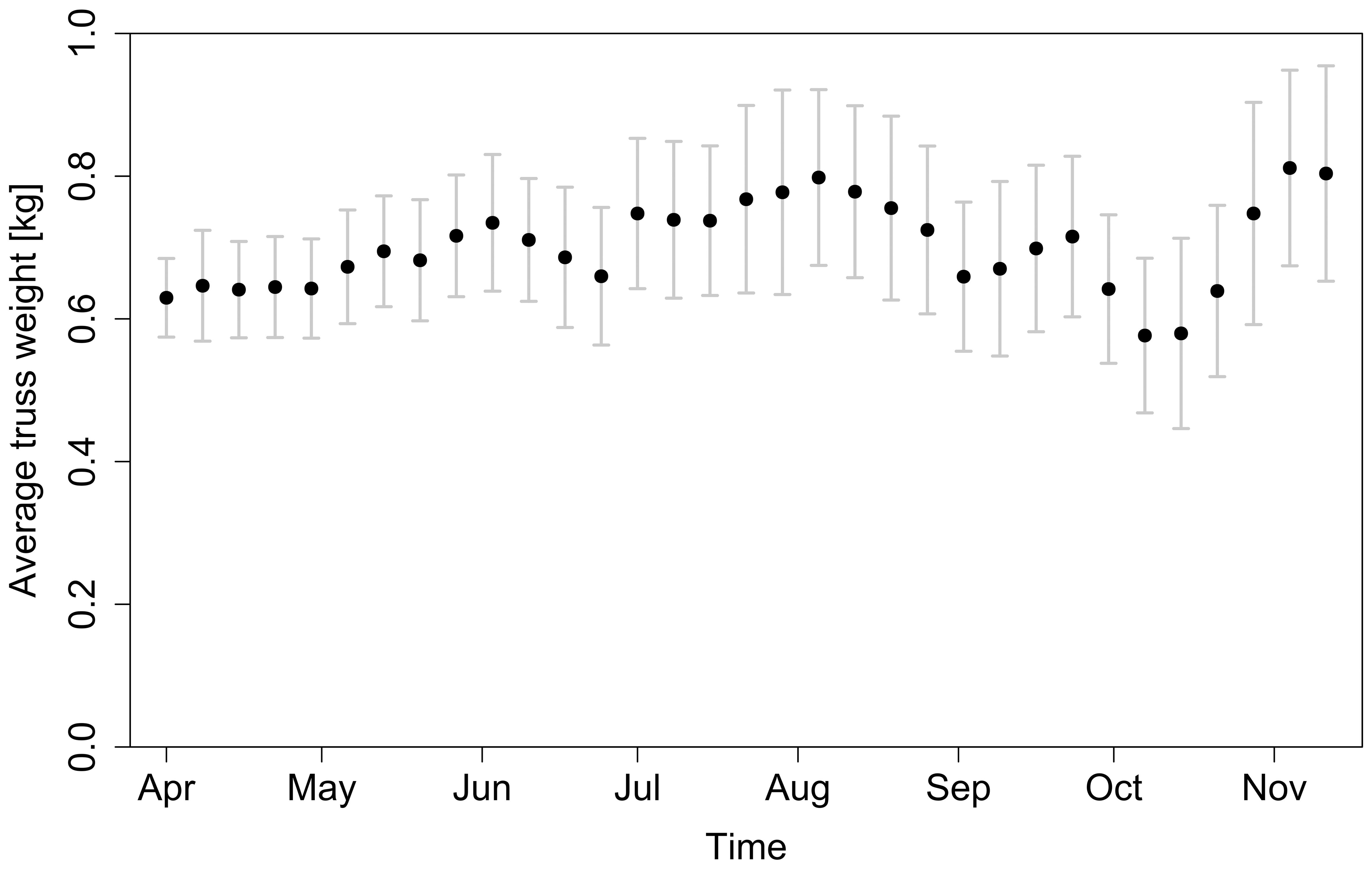
Figure 12. Average truss weight at harvest throughout the whole 2018 season. Error bars represent standard deviation of samples collected for each harvest date.
Our regression models showed an increased explained variance to predict tomato growth when using microclimate GDD compared to using the GDD value from the central weather station (Table 2, Table 3, Figure 9, Figure 10). The output of the ridge model was precise for the average truss fresh weight per harvest day, but with a low explained variance due to variation within individual harvest days (Figure 10A). Various reasons can explain this. There were other environmental factors than temperature and VPD affecting fruit growth, that were not included in the analysis, such as light irradiance (Gautier et al., 2008), CO2 concentration (Jerszurki et al., 2021) or fertigation (Wang and Xing, 2017). Although we assumed uniformity of these factors, local (spatial and temporal) differences most probably exist for them, similar as for the microclimate of temperature and VPD (Critten, 1991; De Rijck and Schrevens, 1998). Apart from environmental factors, a different (micro)climate history accumulated by plants throughout the season might also play a role. Furthermore, management practices also have an effect on plant and fruit growth (Bertin and Génard, 2018). All the mentioned factors are dynamic during the season. The whole-season effects of the environment can be unravelled using mathematical models (Heuvelink, 1996; Jones et al., 1991), which by design allow horizontal microclimate. Observed variability on each harvest day can be either explained by stochastic models (Cooman and Schrevens, 2006; Hall and Gandar, 1995; Tijskens et al., 2016), or by deterministic models with additional factors other than temperature and VPD. Using microclimate data in a PLS analysis did not result in a higher explained variance for fruit quality properties.
4.4 Microclimate differences impact whole-season fruit yield
The fruit growth rate plays an important role when looking at the final yield of the whole season, which is one of the most important elements from a growers’ perspective. The observed difference in fruit growth rate between a warmer and a cooler zone (Figure 11) was present both in summer and autumn with a similar magnitude. This was the case, despite the fact that GDD differences were higher in the autumn period. This can be caused by seasonal differences together with difference in plant properties (e.g., leaf area), accumulated throughout the season, due to variations in microclimate conditions. A similar effect of temperature on fruit growth rate was observed in other studies, however for more pronounced temperature differences – (Adams et al., 2001) up to 12 °C; (Hurd and Graves, 1985) up to 8 °C; (Pearce et al., 1993) up to 10 °C.
In experiments monitoring fruit growth rate (Figure 11) fruits were followed until fully ripe, often beyond the moment of typical harvest. That can explain no significant difference in final weight between microclimate zones, while the opposite was observed when comparing truss weight at harvest (Figure 8). While quality attributes of the harvested fruit were similar between different zones, the local microclimate does affect the number of harvested trusses and thus impacts final yield. Difference in the fruit development rate also affects the homogeneity of harvests.
5 Conclusion
Our study revealed a variable horizontal microclimate within a commercial greenhouse for tomato production. The microclimate distribution was not static but changed during the season, influenced by several factors such as the outside weather or the greenhouse management. The observed variation in temperature and vapour pressure deficit resulted, despite the nature of climate control of a commercial greenhouse, for some periods and locations in suboptimal conditions for plant growth.
A model incorporating these horizontal microclimate effects was able to predict plant stem growth rate and fruit truss weight better, in comparison with a model only using climate data from one central weather station – an indication that the local microclimate impacts plant and fruit development. We found that relatively small, naturally occurring, microclimate differences present in a commercial greenhouse can result in differences in tomato plant and fruit growth, and thus final yield. We did not observe significant differences in fruit quality attributes from different microclimate zones.
Knowledge of a greenhouse’s microclimate is relevant for optimising production. When abandoning the assumption of the presence of a uniform climate within a greenhouse, the use of wireless sensor networks in addition to the central weather station, is an essential and affordable first step to visualize and anticipate microclimate effects. Both vertical and horizontal microclimate should be accounted for.
Data availability statement
The datasets presented in this study can be found in online repositories. The names of the repository/repositories and accession number(s) can be found below: Microclimate monitoring in commercial tomato (Solanum Lycopersicum L.) greenhouse production and its effect on plant growth, yield and fruit quality dataset: https://data.mendeley.com/datasets/tkbkzdt5nr.
Author contributions
JS: Data curation, Formal analysis, Investigation, Methodology, Visualization, Writing – original draft, Writing – review & editing. DV: Data curation, Formal analysis, Investigation, Methodology, Writing – review & editing. PV: Conceptualization, Supervision, Writing – review & editing. KH: Data curation, Investigation, Writing – review & editing. BV: Conceptualization, Data curation, Writing – review & editing. MH: Conceptualization, Investigation, Methodology, Resources, Writing – review & editing. BVP: Conceptualization, Project administration, Resources, Supervision, Writing – review & editing. BN: Conceptualization, Resources, Writing – review & editing.
Funding
The author(s) declare financial support was received for the research, authorship, and/or publication of this article. This research was funded by Interreg Vl-Nl project GROW project. JS acknowledges funding by Research Foundation -Flanders (FWO) as a PhD fellow (project nr. 1SE1921N & 1SE1923N).
Acknowledgments
We would like to thank Tong Guan for her help with data collection for 2020 fruit growth rate measurements.
Conflict of interest
The authors declare that the research was conducted in the absence of any commercial or financial relationships that could be construed as a potential conflict of interest.
Publisher’s note
All claims expressed in this article are solely those of the authors and do not necessarily represent those of their affiliated organizations, or those of the publisher, the editors and the reviewers. Any product that may be evaluated in this article, or claim that may be made by its manufacturer, is not guaranteed or endorsed by the publisher.
Supplementary material
The Supplementary Material for this article can be found online at: https://www.frontiersin.org/articles/10.3389/fhort.2024.1425285/full#supplementary-material
Abbreviations
EC, electric conductivity, (dS m-1); GDD, growing degree days, (°C day); RH, elative humidity, (%); T, temperature, (°C); VP, vapour pressure, (kPa); VPD, vapour pressure deficit, (kPa).
Footnotes
References
Adams S. R., Cockshull K. E., Cave C. R. J. (2001). Effect of temperature on the growth and development of tomato fruits. Ann. botany. 88, 869–877. doi: 10.1006/anbo.2001.1524
Akima H. (1978). A method of bivariate interpolation and smooth surface fitting for irregularly distributed data points. ACM Trans. Math. Software (TOMS). 4, 148–159. doi: 10.1145/355780.355786
Alin A. (2010). Multicollinearity. Wiley Interdiscip. reviews: Comput. statistics. 2, 370–374. doi: 10.1002/wics.84
Alvarez-Sánchez E., Leyva-Retureta G., Portilla-Flores E., López-Velázquez A. (2014). Evaluation of thermal behavior for an asymmetric greenhouse by means of dynamic simulations. Dyna. 81, 152–159. doi: 10.15446/dyna.v81n188.41338
Badji A., Benseddik A., Bensaha H., Boukhelifa A., Hasrane I. (2022). Design, technology, and management of greenhouse: A review. J. Cleaner Production. 373, 133753. doi: 10.1016/j.jclepro.2022.133753
Balendonck J., Os E. A. V., Schoor R., Tuijl B., Keizer L. C. P. (2010). Monitoring spatial and temporal distribution of temperature and relative humidity in greenhouses based on wireless sensor technology. In Proceedings of the International Conference on Agricultural Engineering—AgEng, France: Clermont-Ferrand, 6–8.
Balendonck J., Sapounas A. A., Kempkes F., Van Os E. A., Schoor R., Van Tuijl B. A. J., et al. (2014). Using a wireless sensor network to determine climate heterogeneity of a greenhouse environment. Acta Hortic. 1037, 539–546. doi: 10.17660/ActaHortic.2014.1037.67
Bertin N., Génard M. (2018). Tomato quality as influenced by preharvest factors. Scientia Horticulturae. 233, 264–276. doi: 10.1016/j.scienta.2018.01.056
Bertin N., Guichard S., Leonardi C., Longuenesse J. J., Langlois D., Navez B. (2000). Seasonal evolution of the quality of fresh glasshouse tomatoes under Mediterranean conditions, as affected by air vapour pressure deficit and plant fruit load. Ann. Botany. 85, 741–750. doi: 10.1006/anbo.2000.1123
Bhujel A., Basak J. K., Khan F., Arulmozhi E., Jaihuni M., Sihalath T., et al. (2020). Sensor systems for greenhouse microclimate monitoring and control: a review. J. Biosyst. Engineering. 45, 341–361. doi: 10.1007/s42853-020-00075-6
Bojacá C. R., Gil R., Gómez S., Cooman A., Schrevens E. (2009). Analysis of greenhouse air temperature distribution using geostatistical methods. Trans. ASABE. 52, 957–968. doi: 10.13031/2013.27393
Buck A. L. (1981). New equations for computing vapor pressure and enhancement factor. J. Appl. Meteorology (1962-1982) 20, 1527–1532. doi: 10.1175/1520-0450(1981)020%3C1527:NEFCVP%3E2.0.CO;2
Chen R., Kang S., Hao X., Li F., Du T., Qiu R., et al. (2015). Variations in tomato yield and quality in relation to soil properties and evapotranspiration under greenhouse condition. Scientia Horticulturae. 197, 318–328. doi: 10.1016/j.scienta.2015.09.047
Choab N., Allouhi A., El Maakoul A., Kousksou T., Saadeddine S., Jamil A. (2019). Review on greenhouse microclimate and application: Design parameters, thermal modeling and simulation, climate controlling technologies. Solar Energy. 191, 109–137. doi: 10.1016/j.solener.2019.08.042
Cooman A., Schrevens E. (2006). A Monte Carlo approach for estimating the uncertainty of predictions with the tomato plant growth model, Tomgro. Biosyst. engineering. 94, 517–524. doi: 10.1016/j.biosystemseng.2006.05.005
Critten D. L. (1991). A review of the light transmission into greenhouse crops. Int. Workshop Greenhouse Crop Models 328, 9–32. doi: 10.17660/ActaHortic.1993.328.1
De la Torre-Gea G., Soto-Zarazúa G. M., López-Crúz I., Torres-Pacheco I., Rico-Garcı́a E. (2011). Computational fluid dynamics in greenhouses: A review. Afr. J. Biotechnol. 10, 17651–17662. doi: 10.5897/AJB10.2488
Demers D.-A., Dorais M., Wien C. H., Gosselin A. (1998). Effects of supplemental light duration on greenhouse tomato (Lycopersicon esculentum Mill.) plants and fruit yields. Scientia Horticulturae. 74, 295–306. doi: 10.1016/S0304-4238(98)00097-1
De Rijck G., Schrevens E. (1998). Distribution of nutrients and water in rockwool slabs. Scientia Horticulturae. 72, 277–228. doi: 10.1016/S0304-4238(97)00144-15
FAOSTAT (2020). Production: crops. Available online at: http://www.fao.org/faostat/en/data/QC (Accessed 18 March, 2024).
Farrar D. E., Glauber R. R. (1967). Multicollinearity in regression analysis: the problem revisited. Rev. Economic Stat 49, 92–107. doi: 10.2307/1937887
Ferentinos K. P., Katsoulas N., Tzounis A., Bartzanas T., Kittas C. (2017). Wireless sensor networks for greenhouse climate and plant condition assessment. Biosyst. engineering. 153, 70–81. doi: 10.1016/j.biosystemseng.2016.11.005
Gautier H., Diakou-Verdin V., Bénard C., Reich M., Buret M., Bourgaud F., et al. (2008). How does tomato quality (sugar, acid, and nutritional quality) vary with ripening stage, temperature, and irradiance? J. Agric. Food Chem. 56, 1241–1250. doi: 10.1021/jf072196t
Grange R. I., Hand D. W. (1987). A review of the effects of atmospheric humidity on the growth of horticultural crops. J. Hortic. Science. 62, 125–134. doi: 10.1080/14620316.1987.11515760
Greer D. H., Weedon M. M. (2012). Interactions between light and growing season temperatures on, growth and development and gas exchange of Semillon (Vitis vinifera L.) vines grown in an irrigated vineyard. Plant Physiol. Biochem. 54, 59–69. doi: 10.1016/j.plaphy.2012.02.010
Guichard S., Bertin N., Leonardi C., Gary C. (2001). Tomato fruit quality in relation to water and carbon fluxes. Agronomie. 21, 385–392. doi: 10.1051/agro:2001131
Guzmán C. H., Carrera J. L., Durán H. A., Berumen J., Ortiz A. A., Guirette O. A., et al. (2018). Implementation of virtual sensors for monitoring temperature in greenhouses using CFD and control. Sensors. 19, 60. doi: 10.3390/s19010060
Hall A. J., Gandar P. W. (1995). Stochastic models for fruit growth, IV International Symposium on Computer Modelling in Fruit Research and Orchard Management. Acta Horticulturae. 416, 113–120. doi: 10.17660/ActaHortic.1996.416.13
Heuvelink E. (1996). Tomato growth and yield: quantitative analysis and synthesis (Wageningen: Wageningen University and Research).
Hoerl A. E., Kennard R. W. (1970). Ridge regression: applications to nonorthogonal problems. Technometrics. 12, 69–82. doi: 10.1080/00401706.1970.10488635
Holsteens K., Moerkens R., Van de Poel B., Vanlommel W. (2020). The effect of low-haze diffuse glass on greenhouse tomato and bell pepper production and light distribution properties. Plants. 9, 806. doi: 10.3390/plants9070806
Hurd R. G., Graves C. J. (1985). Some effects of air and root temperatures on the yield and quality of glasshouse tomatoes. J. Hortic. Science. 60, 359–371. doi: 10.1080/14620316.1985.11515640
Hwang H., An S., Pham M. D., Cui M., Chun C. (2020). The combined conditions of photoperiod, light intensity, and air temperature control the growth and development of tomato and red pepper seedlings in a closed transplant production system. Sustainability. 12, 9939. doi: 10.3390/su12239939
Inoue T., Yamori W. (2021). Minimizing VPD fluctuations maintains higher stomatal conductance and photosynthesis, resulting in improvement of plant growth in lettuce. Front. Plant Science. 12. doi: 10.3389/fpls.2021.646144
Jerszurki D., Saadon T., Zhen J., Agam N., Tas E., Rachmilevitch S., et al. (2021). Vertical microclimate heterogeneity and dew formation in semi-closed and naturally ventilated tomato greenhouses. Scientia Horticulturae. 288, 110271. doi: 10.1016/j.scienta.2021.110271
Jewett T., Jarvis W. (2001). Management of the greenhouse microclimate in relation to disease control: a review. Agronomie. 21, 351–366. doi: 10.1051/agro:2001129
Jones J. W., Dayan E., Allen L. H., Van Keulen H., Challa H. (1991). A dynamic tomato growth and yield model (TOMGRO). Trans. ASAE. 34, 663–0672. doi: 10.13031/2013.31715
Kempkes F. L. K., Van de Braak N. J., Bakker J. C. (2000). Effect of heating system position on vertical distribution of crop temperature and transpiration in greenhouse tomatoes. J. Agric. Eng. Res. 75, 57–64. doi: 10.1006/jaer.1999.0485
Kim S. E., Lee M. Y., Lee M. H., Sim S. Y., Kim Y. S. (2014). Optimal management of tomato leaf pruning in rockwool culture. Horticulture Environment Biotechnol. 55, 445–454. doi: 10.1007/s13580-014-0049-y
Kimura K., Yasutake D., Koikawa K., Kitano M. (2023). Spatiotemporally variable incident light, leaf photosynthesis, and yield across a greenhouse: fine-scale hemispherical photography and a photosynthesis model. Precis. Agriculture. 24, 114–138. doi: 10.1007/s11119-016-9492-3
Kittas C., Bartzanas T. (2007). Greenhouse microclimate and dehumidification effectiveness under different ventilator configurations. Building Environment. 42, 3774–3784. doi: 10.1016/j.buildenv.2006.06.020
Kittas C., Karamanis M., Katsoulas N. (2005). Air temperature regime in a forced ventilated greenhouse with rose crop. Energy buildings. 37, 807–812. doi: 10.1007/s13580-014-0049-y
Kutta E., Hubbart J. (2014). Improving understanding of microclimate heterogeneity within a contemporary plant growth facility to advance climate control and plant productivity. Plant Sci. 2, 167–178. doi: 10.11648/j.jps.20140205.14
Lamprinos I., Charalambides M., Chouchoulis M. (2015). “Greenhouse monitoring system based on a wireless sensor network,” in Proceedings of the 2nd International Electronic Conference on Sensors and Applications. 13–15. doi: 10.3390/ecsa-2-E009
Legast E., Brajeul E., Truffault V. (2019). “Effect of temperature on tomato fruit growth: a modelling-based proposal for optimal temperature distribution within heated greenhouse,” in International Symposium on Advanced Technologies and Management for Innovative Greenhouses: GreenSys2019, Vol. 1296. 49–56. doi: 10.17660/ActaHortic.2020.1296.7
Levene H. (1960). Robust tests for equality of variances. Contributions to probability Stat 69, 278–292.
Lu N., Nukaya T., Kamimura T., Zhang D., Kurimoto I., Takagaki M., et al. (2015). Control of vapor pressure deficit (VPD) in greenhouse enhanced tomato growth and productivity during the winter season. Scientia Horticulturae. 197, 17–23. doi: 10.1016/j.scienta.2015.11.001
Marquardt D. W., Snee R. D. (1975). Ridge regression in practice. Am. Statistician. 29, 3–20. doi: 10.1080/00031305.1975.10479105
Muñoz M., Guzmán J. L., Sánchez J. A., Rodrı́guez F., Torres M. (2019). Greenhouse models as a service (GMaaS) for simulation and control. IFAC-PapersOnLine. 52, 190–195. doi: 10.1016/j.ifacol.2019.12.520
Nkansah G. O., Amoatey C., Zogli M. K., Owusu-Nketia S., Ofori P. A., Opoku-Agyemang F. (2021). Influence of topping and spacing on growth, yield, and fruit quality of tomato (Solanum lycopersicum L.) under greenhouse condition. Front. Sustain. Food Systems. 5. doi: 10.3389/fsufs.2021.659047
Ogunlowo Q. O., Akpenpuun T. D., Na W.-H., Rabiu A., Adesanya M. A., Addae K. S., et al. (2021). Analysis of heat and mass distribution in a single-and multi-span greenhouse microclimate. Agriculture. 11, 891. doi: 10.3390/agriculture11090891
Panwar N. L., Kaushik S. C., Kothari S. (2011). Solar greenhouse an option for renewable and sustainable farming. Renewable Sustain. Energy Rev. 15, 3934–3945. doi: 10.1016/j.rser.2011.07.030
Pathak T. B., Stoddard C. S. (2018). Climate change effects on the processing tomato growing season in California using growing degree day model. Modeling Earth Syst. Environment. 4, 765–775. doi: 10.1007/s40808-018-0460-y
Pawlowski A., Guzman J. L., Rodrı́guez F., Berenguel M., Sánchez J., Dormido S. (2009). Simulation of greenhouse climate monitoring and control with wireless sensor network and event-based control. Sensors. 9, 232–252. doi: 10.3390/s90100232
Pearce B. D., Grange R. I., Hardwick K. (1993). The growth of young tomato fruit. I. Effects of temperature and irradiance on fruit grown in controlled environments. J. Hortic. Science. 68, 1–11. doi: 10.1080/00221589.1993.11516322
Picken A. J. F. (1984). A review of pollination and fruit set in the tomato (Lycopersicon esculentum Mill.). J. Hortic. Science. 59, 1–13. doi: 10.1080/00221589.1984.11515163
Qian T., Dieleman J. A., Elings A., De Gelder A., Marcelis L. F. M. (2015). Response of tomato crop growth and development to a vertical temperature gradient in a semi-closed greenhouse. J. Hortic. Sci. Biotechnol. 90, 578–584. doi: 10.1080/14620316.2015.11668717
Reichrath S., Davies T. W. (2002). Using CFD to model the internal climate of greenhouses: past, present and future. Agronomie. 22, 3–19. doi: 10.1051/agro:2001006
Rezvani S.-e., Abyaneh H. Z., Shamshiri R. R., Balasundram S. K., Dworak V., Goodarzi M., et al. (2020). IoT-based sensor data fusion for determining optimality degrees of microclimate parameters in commercial greenhouse production of tomato. Sensors. 20, 6474. doi: 10.3390/s20226474
Riga P., Anza M., Garbisu C. (2008). Tomato quality is more dependent on temperature than on photosynthetically active radiation. J. Sci. Food Agriculture. 88, 158–166. doi: 10.1002/jsfa.3065
Rodrı́guez F., Berenguel M., Guzmán J. L., Ramı́rez-Arias A. (2015). Modeling and control of greenhouse crop growth (Basel: Springer). doi: 10.1007/978-3-319-11134-6
Roltsch W. J., Zalom F. G., Strawn A. J., Strand J. F., Pitcairn M. J. (1999). Evaluation of several degree-day estimation methods in California climates. Int. J. Biometeorology. 42, 169–176. doi: 10.1007/s004840050101
Rubinetti D., Iranshahi K., Onwude D. I., Xie L., Nicolaıü B., Defraeye T. (2023). An in-silico proof-of-concept of electrohydrodynamic air amplifier for low-energy airflow generation. J. Cleaner Production. 398, 136531. doi: 10.1016/j.jclepro.2023.136531
Salagovic J., Vanhees D., Verboven P., Holsteens K., Verlinden B., Huysmans M., et al. (2024). Microclimate monitoring in commercial tomato (Solanum Lycopersicum L.) greenhouse production and its effect on plant growth, yield and fruit quality dataset. Mendeley Data. doi: 10.17632/tkbkzdt5nr.2
Saltveit M. E. (1999). Effect of ethylene on quality of fresh fruits and vegetables. Postharvest Biol. technology. 15, 279–292. doi: 10.1016/S0925-5214(98)00091-X
Sethi V. P., Sharma S. K. (2007). Survey of cooling technologies for worldwide agricultural greenhouse applications. Solar Energy. 81, 1447–1459. doi: 10.1016/j.solener.2007.03.004
Shamshiri R. R., Bojic I., van Henten E., Balasundram S. K., Dworak V., Sultan M., et al. (2020). Model-based evaluation of greenhouse microclimate using IoT-Sensor data fusion for energy efficient crop production. J. Cleaner Production. 263, 121303. doi: 10.1515/intag-2017-0005
Shamshiri R. R., Jones J. W., Thorp K. R., Ahmad D., Man H. C., Taheri S. (2018). Review of optimum temperature, humidity, and vapour pressure deficit for microclimate evaluation and control in greenhouse cultivation of tomato: a review. Int. agrophysics. 32, 287–302. doi: 10.1016/j.jclepro.2020.121303
Shapiro S. S., Wilk M. B. (1965). An analysis of variance test for normality (complete samples). Biometrika. 52, 591–611. doi: 10.2307/2333709
Singh R. K., Aernouts M., De Meyer M., Weyn M., Berkvens R. (2020). Leveraging LoRaWAN technology for precision agriculture in greenhouses. Sensors. 20, 1827. doi: 10.3390/s20071827
Su Y., Xu L. (2017). Towards discrete time model for greenhouse climate control. Eng. agriculture Environ. Food. 10, 157–170. doi: 10.1016/j.eaef.2017.01.001
Suay R., López S., Granell R., Moltó E., Fatnassi H., Boulard T. (2008). Preliminary analysis of greenhouse microclimate heterogeneity for different weather conditions Vol. 797 (International Workshop on Greenhouse Environmental Control and Crop Production in Semi-Arid Regions), 103–109. doi: 10.17660/ActaHortic.2008.797.12
Tijskens L. M. M., Unuk T., Okello R. C. O., Wubs A. M., Šuštar V., Šumak D., et al. (2016). From fruitlet to harvest: Modelling and predicting size and its distributions for tomato, apple and pepper fruit. Scientia Horticulturae. 204, 54–64. doi: 10.1016/j.scienta.2016.03.036
Wang X., Xing Y. (2017). Evaluation of the effects of irrigation and fertilization on tomato fruit yield and quality: a principal component analysis. Sci. Rep. 7, 350. doi: 10.1038/s41598-017-00373-8
Keywords: tomato, microclimate, temperature, vapour pressure deficit, yield, fruit quality
Citation: Šalagovič J, Vanhees D, Verboven P, Holsteens K, Verlinden B, Huysmans M, Van de Poel B and Nicolaï B (2024) Microclimate monitoring in commercial tomato (Solanum Lycopersicum L.) greenhouse production and its effect on plant growth, yield and fruit quality. Front. Hortic. 3:1425285. doi: 10.3389/fhort.2024.1425285
Received: 29 April 2024; Accepted: 23 September 2024;
Published: 07 October 2024.
Edited by:
Xiangming Xu, National Institute of Agricultural Botany (NIAB), United KingdomReviewed by:
Georgios K. Ntinas, Hellenic Agricultural Organization – ELGO, GreeceMargit Olle, NPO Veggies cultivation, Estonia
Copyright © 2024 Šalagovič, Vanhees, Verboven, Holsteens, Verlinden, Huysmans, Van de Poel and Nicolaï. This is an open-access article distributed under the terms of the Creative Commons Attribution License (CC BY). The use, distribution or reproduction in other forums is permitted, provided the original author(s) and the copyright owner(s) are credited and that the original publication in this journal is cited, in accordance with accepted academic practice. No use, distribution or reproduction is permitted which does not comply with these terms.
*Correspondence: Bram Van de Poel, YnJhbS52YW5kZXBvZWxAa3VsZXV2ZW4uYmU=; Bart Nicolaï, YmFydC5uaWNvbGFpQGt1bGV1dmVuLmJl