Efficiently solving open capacitated location-routing problems through a discrete fireworks algorithm

In the open capacitated location-routing problem (OCLRP), a fleet of distribution vehicles departs from selected depots to satisfy customers’ demands, but they do not need to return to their starting depots after serving all customers. Comparing the solutions of the OCLRP and its corresponding capacitated location-routing problem (CLRP) can provide valuable insights for companies considering whether to outsource their delivery activities. To effectively solve the OCLRP, this study proposes a novel discrete fireworks algorithm (DFWA) with two key innovations. (1) An adaptive search mechanism: embedding swap, insertion, and reverse operations into explosion/mutation breaks the limitations of traditional fireworks algorithms in discrete optimization by expanding the search space while enhancing local tuning, thus boosting global optimal solution discovery. (2) A diversified selection strategy: integrating fitness value and Hamming distance improves the “premature convergence from single fitness selection” defect in existing algorithms. It retains high-performance solutions while maintaining population diversity. Evaluated on OCLRP instances adapted from standard CLRP benchmarks, the DFWA shows strong competitiveness, consistently generating high-quality solutions within reasonable computation time. A real-world OCLRP case further verifies its practical applicability in complex industrial scenarios.

1 Introduction

In the current highly competitive economic environment, companies aim for improved supply chain management, including efficient decision-making about depot locations and delivery route design, as these may entail important cost and time savings (Dai, Aqlan, Gao and Zhou, 2019; Zhang et al., 2022b). As a consequence, there is extensive research on both facility location (FLP) (Garcia-Diaz and Smith, 2024) and vehicle routing (VRP) (Niu, Shao, Xiao, Song and Cao, 2022; Zhang et al., 2022a; Garside, Ahmad and Muhtazaruddin, 2024) problems. However, solving these problems as silos may lead to inferior solutions. Location routing problems (LRP) combine both problems and typically lead to more flexible and efficient logistics systems (Mohamed, Klibi, Sadykov, Sen and Vanderbeck, 2022; Yu and Lin, 2015).

A major consequence of the current competitive environment is that companies are increasingly focusing on their core value-added capabilities and activities and tend to outsource their logistics to third-party (TPL) providers (Yu and Lin, 2015). In such cases, TPL provider vehicles usually start their service from the company’s depots (or distribution centers) and return to the TPL installations instead of the depots or distribution centers after delivering to customers; consequently, classic capacitated location-routing problems (CLRPs) are not applicable. To handle these situations, open capacitated location routing problems (OCLRPs) were proposed by Yu and Lin (2015). OCLRPs do not consider the costs associated with the starting trip from the TPL company to its depot nor the return trip from a vehicle’s last customer to the TPL facilities. Thus, the company only considers the costs of locating its depots and those associated with the number of hired vehicles and the trips between depots and the last customer that the vehicle served (Nucamendi-Guillén, Padilla and Moreno-Vega, 2021).

This study provides a novel approach to OCLRPs. We assume that each candidate depot and vehicle have limited capacities and that vehicles return to TPL installations instead of the company’s depots after having served their last customer. OCLRPs simultaneously search for depot locations and vehicle routes to satisfy customers’ demands. The main difference between CLRPs and OCLRPs is that each route in an OCLRP is a Hamiltonian path (vehicles do not return to the starting depot), whereas each route in a CLRP is a Hamiltonian cycle (vehicles return to the starting depot) (Yu and Lin, 2015). Figure 1 illustrates the differences between CLRP and OCLRP solutions in a problem with three depots (triangles), nine customers (circles), and three routes. Both solutions are constructed on a complete directed graph $G=(V,E)$ where the vertex set $E=\{<i,j>|i,j\in V,i\ne j\}$. Critically, the cost of each arc $<i,j>\in E$ corresponds to the straight-line distance between the spatial positions of vertex $i$ and vertex $j$ (spatial positions of all points are meaningful for route cost calculation). In Figure 1, for visual clarity (especially in printed form), we use solid arcs to represent the OCLRP solution (Hamiltonian paths starting from depots and ending at customers) and solid arcs plus red dashed arcs to represent the corresponding CLRP solution (Hamiltonian cycles that return to the starting depot after serving all customers on the route).

Figure 1

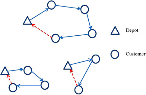
Figure 1. CLRP and OCLRP solutions with three depots, three routes, and nine customers.

Importantly, the difference between the solution values of a CLRP and its corresponding OCLRP provides a benchmark to support a company’s decision on whether to outsource delivery activities (Yu and Lin, 2015). While OCLRP and CLRP solutions only differ in the “depot–last customer” arc cost (OCLRP omits this cost), a good CLRP cycle does not guarantee a good OCLRP path; this is because the optimal OCLRP path depends on both inter-customer distances and customer–depot distance, rather than just the closed-loop cost of CLRP. Figure 2 further validates this discrepancy, where 2(a) shows the optimal solution of a CLRP and 2(b) shows the optimal solution of its corresponding OCLRP (both with three candidate depots and nine customers). In Figure 2, depots are marked as triangles and customers are marked as circles. Both 2(a) and 2(b) are built on the same weighted complete directed graph, so that their vertex set, spatial positions of all vertices, and arc costs (straight-line distances) are identical. Solid arcs in Figure 2a form three CLRP cycles, while the red dashed arcs in Figure 2b form two OCLRP paths. This figure helps illustrate that the optimal solution for an OCLRP cannot simply be derived by removing the edge between the depot and the last customer from the optimal solution of the CLRP.

Figure 2

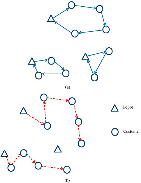
Figure 2. Illustration of the differences between the optimal solutions of a CLRP and that of its corresponding OCLRP. (a) Optimal solution of CLRP instance. (b) Optimal solution of OCLRP instance.

As the VRP (Ergao and Mingyong, 2009) and FLP (Garcia-Diaz and Smith, 2024) are both NP-hard problems, so the CLRP is also NP-hard (Dai et al., 2019). Given its important practical applications and high computational complexity, the CLRP has attracted the interest of numerous researchers who have proposed a wide variety of algorithms, including genetic algorithms (Bootaki and Zhang, 2024; Arifuddin, Utamima, Mahananto, Vinarti and Fernanda, 2024), simulated annealing (SA) (Ferreira and Alves de Queiroz, 2022), particle swarm optimization (Kechmane, Nsiri and Baalal, 2018; Wang et al., 2021), tabu search (Kyriakakis, Sevastopoulos, Marinaki and Marinakis, 2022), ant colony optimization (Ting and Chen, 2013), greedy randomized adaptive search procedures (Prins, Prodhon and Calvo, 2006), and memetic algorithms with population management (Shi, Zhou, Boudouh and Grunder, 2022). Moreover, some exact algorithms have been also proposed, based on dynamic programming, column generation (Farham, Süral and Iyigun, 2018), branch-and-cut (Marques, Sadykov, Deschamps and Dupas, 2020), and branch pricing algorithms. In contrast, the OCLRP has received comparatively less attention, and there is still much scope to improve available models and solutions. Nucamendi-Guillén et al. (2021) proposed a multi-start metaheuristic algorithm to solve the multi-depot open location routing problem with a heterogeneous fixed fleet. Yu and Lin (2015) proposed an effective simulated annealing heuristic for solving OCLRPs based on a special solution representation enlarging the search space and facilitating its exploration. Toro, Franco, Granada-Echeverri, Guimarães, and Rendón (2016) took into account current environmental issues and proposed the green open location-routing problem. Nucamendi-Guillén et al. (2021) were inspired by a real case and proposed a multi-depot OLRP with a fixed heterogeneous fleet.

As a variant of the CLRP, the OCLRP retains the same computational challenge. Moreover, existing mainstreams for similar routing problems face notable limitations when adapted to the OCLRP’s unique characteristics (i.e., Hamiltonian path constraints and depot–customer–vehicle coupling). For instance, simulated annealing heuristics such as proposed by Yu and Lin (2015) expand the search space via special solution representation but often stagnate in local optima for large-scale instances (e.g., 100+ customers), as their single-solution iterative update lacks sufficient local exploitation. Genetic algorithms, though widely applied to the CLRP (Bootaki and Zhang, 2024), struggle with the OCLRP’s path-specific constraints, as their crossover operators often disrupt valid route structures, leading to a high proportion of infeasible solutions that require additional repair mechanisms. Even neighborhood-based methods such as adaptive large neighborhood search (ALNS) and tabu search (TS), while excellent at neighborhood exploration for VRPs, lack the targeted handling of the OCLRP’s triple coupling of depot selection, customer assignment, and vehicle routing, resulting in inefficient search processes and suboptimal cost performance.

In contrast, fireworks algorithms (FWAs) have shown accurate and consistent performance in complex optimization (Y. Tan and Zhu, 2010; Chen et al., 2019) but are rarely applied to NP-hard combinatorial problems like OCLRP, FLP, VRP, or LRP and their variants. This study aims to fill this gap by proposing a novel discrete fireworks algorithm (DFWA) for solving the OCLRP, motivated by three key advantages of the FWA. First, as a heuristic approach, the FWA provides an effective algorithmic framework that delivers acceptable solutions in reasonable computing time to NP-hard optimization problems (Niu et al., 2022). Second, as a meta-heuristic, it allows the flexible integration of local search operators (Zhang et al., 2019; Tan et al., 2025)—a feature that can mitigate SA’s local stagnation and GA’s infeasibility issues. Third, the performance of FWAs have been found accurate and consistent, and they can achieve competitive results in comparison to other well-known optimization algorithms (Tan and Zhu, 2010; Chen et al., 2019). They have been applied in domains such as multimodal function optimization (Meng and Tan, 2024), radar deployment for UAV swarms defense coverage (Ding et al., 2025), and heterogeneous multi-project multi-task allocation in mobile crowdsensing (Shen et al., 2023), indicating their potential to handle the OCLRP’s complex constraints.

The key contributions of this study are the following. Firstly, it proposes a mathematical programming model for the OCLRP. Second, it presents an efficient DFW algorithm for solving the OCLRP. This entails providing an effective initialization and convenient explosion and mutation operators to respectively enhance the exploitation and exploration of the search space. Third, in-depth numerical experiments are conducted to facilitate parameter choice and evaluate the operational gains obtained using the proposed OCLRP model and DFWA. Such experiments and a real case study clearly showcase the effectiveness of our proposal.

The rest of this study covers the following issues. Section 2 states the details of the OCLRP model. Section 3 proposes and discusses our DFWA. Section 4 then provides an in-depth computational analysis, including a real case study. Conclusions and future research are presented in Section 5.

2 Mathematical model for the OCLRP

We present here the formulation of the OCLRP for which we shall develop an efficient algorithm. A set of customers with known locations is available. Their known demands should be satisfied from a set of depots with known locations and opening costs. For this, there is a fleet of homogeneous vehicles with known capacity. Customers must be serviced once, and only once, by a single vehicle. A route load cannot exceed the vehicle capacity, with each route starting from a depot and ending at a customer. Similarly, the demands allocated to a depot cannot surpass its capacity. The OCLRP is typically formulated to minimize total distribution costs, which cover the costs of opening the depots, the fixed vehicle costs, and the routing costs.

The underlying structure to formulate the problem is a complete directed graph $(V,E)$. Its vertex set $V$ is $V_p\bigcup V_d\bigcup V_c$ where $V_p$, $V_d$, and $V_c$, respectively, represent the set of locations of the parking lots of the TPL company, of $m$ candidate depots, and of $n$ customers. Its arc set is $E=\{⟨i,j⟩|i,j\in V\mathrm{a}\mathrm{n}\mathrm{d}i\ne j\}$. The rest of the notation is as follows.

Sets and parameters:

$V_d$: $=\{\mathrm{1,2},\dots ,m\}$.

$V_c$: $=\{m+1,m+2,\dots ,m+n\}$.

$K$: set of homogeneous vehicles with common capacity $P$.

$O_i$: $i$-th depot fixed opening cost.

$d_i$: $i$-th customer demand.

$Q_i$: $i$-th depot capacity.

$c_{ij}$: distance from node $i$ to node $j$.

$e$: transportation cost per unit distance.

$w$: vehicle fixed cost.

Decision Variables:

$\begin{array}{ll}\hfill x_{\mathit{ijk}}& =\left\{\begin{array}{cc}1,\hfill & \text{if\hspace{0.17em}}k-\text{th\hspace{0.17em}vehicle\hspace{0.17em}travels\hspace{0.17em}directly\hspace{0.17em}from\hspace{0.17em}}i-\text{th\hspace{0.17em}to\hspace{0.17em}}j-\text{th\hspace{0.17em}node.}\hfill \\ 0,\hfill & \text{otherwise\hspace{0.17em}}\hfill \end{array}\right.\hfill \\ \hfill y_{ij}& =\left\{\begin{array}{cc}1,\hfill & \text{if\hspace{0.17em}}j-\text{th\hspace{0.17em}customer\hspace{0.17em}is\hspace{0.17em}served\hspace{0.17em}by\hspace{0.17em}}i-\text{th\hspace{0.17em}depot.}\hfill \\ 0,\hfill & \text{otherwise\hspace{0.17em}}\hfill \end{array}\right.\hfill \\ \hfill z_i& =\left\{\begin{array}{cc}1,\hfill & \text{if\hspace{0.17em}}i-\text{th\hspace{0.17em}depot\hspace{0.17em}is\hspace{0.17em}opened.}\hfill \\ 0,\hfill & \text{otherwise\hspace{0.17em}}\hfill \end{array}\right.\hfill \\ \hfill u_{jk}& :\text{Auxiliary\hspace{0.17em}variables\hspace{0.17em}for\hspace{0.17em}sub}-\text{tour\hspace{0.17em}elimination\hspace{0.17em}constraints\hspace{0.17em}in\hspace{0.17em}route\hspace{0.17em}}k\text{.\hspace{0.17em}}\hfill \end{array}$

Using the above notation, the OCLRP may be modeled through the following integer linear programming problem:

$\min {\displaystyle \sum _{i\in V_d}}{O}_i{z}_i+{\displaystyle \sum _{i\in V_d}}{\displaystyle \sum _{j\in V_c}}{\displaystyle \sum _{k\in K}}w{x}_{\mathit{ijk}}+{\displaystyle \sum _{i\in V_d\bigcup V_c}}{\displaystyle \sum _{j\in V_c}}{\displaystyle \sum _{k\in K}}{c}_{ij}e{x}_{\mathit{ijk}}(1)$

subject to:

${\displaystyle \sum _{i\in V_d\bigcup V_c}}{\displaystyle \sum _{k\in K}}{x}_{\mathit{ijk}}=1\forall j\in V_c(2)$

${\displaystyle \sum _{i\in V_d\bigcup V_c}}{\displaystyle \sum _{j\in V_c}}{d}_j{x}_{\mathit{ijk}}\le P\forall k\in K(3)$

${\displaystyle \sum _{j\in V_c}}{d}_j{y}_{ij}\le Q_i{z}_i\forall i\in V_d(4)$

${\displaystyle \sum _{i\in V_d\bigcup V_c}}{x}_{\mathit{ijk}}-{\displaystyle \sum _{i\in V_c\bigcup V_p}}{x}_{\mathit{jik}}=0\forall j\in V_c,\forall k\in K(5)$

${\displaystyle \sum _{i\in V_d}}{\displaystyle \sum _{k\in K}}{x}_{\mathit{ijk}}={\displaystyle \sum _{i\in V_d}}{\displaystyle \sum _{k\in K}}{x}_{\mathit{jik}}=0\forall j\in V_d(6)$

${\displaystyle \sum _{j\in V_d}}{x}_{\mathit{ijk}}=0\forall i\in V_c,\forall k\in K(7)$

${\displaystyle \sum _{i\in V_d}}{y}_{ij}=1\forall j\in V_c(8)$

${\displaystyle \sum _{j\in V_c}}{x}_{\mathit{ijk}}-z_i\le 0\forall i\in V_d,\forall k\in K(9)$

$u_{lk}-u_{jk}+n{x}_{\mathit{ljk}}\le n-1\forall l\in V_c,\forall j\in V_c,\forall k\in K(10)$

$x_{\mathit{ijk}}\in \left\{\mathrm{0,1}\right\}\forall i\in V_d\cup V_c,\forall j\in V_p\cup V_c,\forall k\in K(11)$

$y_{ij}\in \left\{\mathrm{0,1}\right\}\forall i\in V_d,\forall j\in V_c(12)$

$z_i\in \left\{\mathrm{0,1}\right\}\forall i\in V_d(13)$

$u_{jk}\in \left\{\mathrm{0,1,2},\dots ,n\right\}\forall j\in V_c,\forall k\in K(14)$

As mentioned, the objective function (1) aggregates the costs of opening the depots, the fixed costs of employing vehicles, and the routing costs. Constraint (2) reflects the fact that customers are serviced only once by one vehicle and that they should have just one predecessor. Constraints (3) and (4) ensure, correspondingly, that vehicle and depot capacities are respected. Route continuity is guaranteed through constraint (5). In turn, constraint (6) models the fact that there should be no connection between any two depots, and constraint (7) that each route ends at the last customer. The group of constraints (8) models the issue that each and any customer should be assigned to exactly one depot, whereas (9) guarantees the fact that vehicles dispatch from depots that are open. Constraint (10) eliminates sub-tours within vehicle routes. Finally, constraints (11)–(13) specify the binary character of some of the variables, and (14) is auxiliary variables.

3 Discrete fireworks algorithm for the OCLRP

To facilitate understanding of the proposed algorithm, we first clarify two core technical terms specific to a fireworks algorithm (FWA). (a) Firework: each firework represents a feasible solution within the search space. (b) Spark: a spark is a new candidate solution generated by applying algorithm-specific operators (e.g., explosion) to an existing firework. Sparks represent potential improvements over the original firework, and their quality is evaluated via the fitness function, which in this study is defined as the OCLRP’s objective function.

Tan and Zhu (2010) and Tan (2015) introduced the FWA for optimization problems, inspired by how fireworks explosions resemble optimal solution searches in swarm intelligence algorithms, with each spark generated by a firework explosion assimilated to a feasible solution. It runs iteratively according to the following scheme until certain stopping conditions are met. For each explosion generation, $N$ fireworks are set off from $N$ given locations, from which a certain number of sparks are generated and their fitness assessed. The number and amplitude of the sparks depend on the explosion operator implemented, with some further sparks generated through a mutation operator. A mapping rule eventually maps infeasible sparks into feasible ones. Lastly, a selection strategy is used to select $N$ sparks for the next explosion generation. The original FWA was designed for continuous optimization problems and cannot be directly used to solve the OCLRP (and other discrete optimization problems). For this, we need to modify the explosion and mutation operators used to explore the feasible space.

We now present a DFWA to efficiently solve OCLRPs. The basic steps of our DFWA for solving the OCLRP are presented as pseudocode in Algorithm 1. The input to the algorithm includes the maximum number $G$ of iterations, the number $N$ of fireworks, the number $Musparks$ of mutation sparks, the maximum explosion amplitude $\widehat{A}$, and a coefficient $\widehat{M}$ controlling the number of explosion sparks generated by each firework. After the fireworks’ initialization (line 1), each firework’s fitness is assessed (line 2) and the best one is determined (line 3). Lines 4–22 cover the DFWA iterations, including the initialization of the sets of sparks generated by the explosion and mutation operators (line 5), the generation of explosion sparks (lines 6–10), the update of individuals (lines 11 and 19), the calculation of the number of fireworks and explosion sparks (line 12), the generation of mutation sparks (lines 13–18), the resetting of the best individual (line 20), and the selection of the next generation of sparks (line 21). Note that the mapping rule is called upon in lines 9 and 16. To facilitate understanding, Figure 3 illustrates the overall logical flow of the algorithm. The forthcoming subsections provide core algorithmic details.

Figure 3

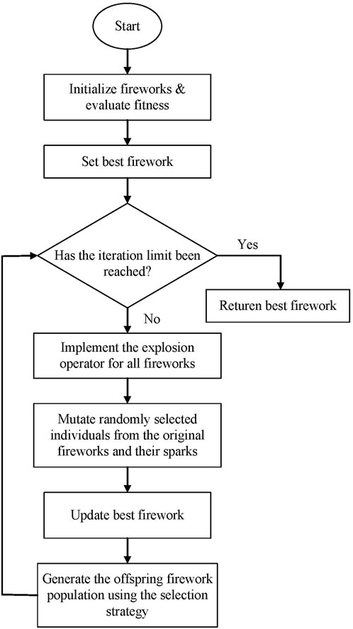
Figure 3. Flowchart of discrete fireworks algorithm for OCLRP.

Algorithm 1

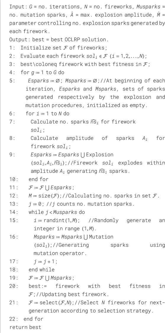
Algorithm 1. Discrete fireworks algorithm for the OCLRP.

3.1 Representation of OCLRP solutions

A compact solution representation is crucial for efficiently implementing a DFWA. In the OCLRP, it should characterize the customer–vehicle assignment, the chosen depots, and the sequence of customers served by a specific vehicle starting at a given depot. Given $m$ and $n$, our representation uses $N_{\text{dummy}}$ dummy zeros (with $N_{\text{dummy}}\le \lceil {\sum }_{i\in V_c}(d_i)/P\rceil$, where $\lceil x\rceil$ represents the ceiling of $x$) and all of the elements within sets $V_d$ and $V_c$. The first number in the representation is in $V_d$ and indicates the first depot in the route; then the customers assigned to each depot appear between it and the next different depot in the order they are serviced, respecting the vehicle capacity constraint. No customers after a depot indicates that such a depot is not open. The end of a route and the start of a new one are marked with dummy zeros, even if additional customers may be served by a vehicle with sufficient capacity. Thus, vehicle routes can be randomly terminated with dummy zeros in the representation. As a consequence, the search space is larger and better solutions can be found (Yu and Lin, 2015; Yu and Lin, 2016).

As an illustration, Figure 4 presents a feasible solution of an OCLRP with five depots and 21 customers. Observe that depot 1 is not open (no customers after it). The routes served from the four open depots (2, 3, 4, 5) are

$•$ D 5$\to$c 10$\to$c 9$\to$c 16.

$•$ D 2$\to$c 6$\to$c 12$\to$c 13$\to$c 24$\to$c 23$\to$c 14$\to$c 26.

$•$ D 3$\to$c 17$\to$c 25$\to$c 7$\to$c 8$\to$c 11.

$•$ D 3$\to$c 22$\to$c 21$\to$c 19$\to$c 15.

$•$ D 4$\to$c 18$\to$c 20.

Figure 4

Figure 4. Example of solution representation.

3.2 DFWA initial solutions

We construct a set of good initial solutions by randomly generating the open depots and assigning their customers with a greedy approach that promotes use of the maximum capacity of a vehicle; this initialization process corresponds to line 1 of Algorithm 1 (”Initialize set $\mathcal{F}$ of fireworks”). The detailed steps are as follows:

Step 1. Randomly generate a permutation $Per$ of the $m$ depots in $V_d$. Denote the $i$-th element in $Per$ as $pe{r}_i$ and set $i=1$. Let $C$ be the full set of all customers in $V_c$. Since no customer is assigned initially, set $Cus≔C$ (where $Cus$ represents the set of unassigned customers).

Step 2. Designate $C(pe{r}_i)\subseteq Cus$ as the subset of unassigned customers whose individual demands do not exceed the remaining capacity of $pe{r}_i$. To initially allocate the unassigned customers and start a new route from $pe{r}_i$, its closest customer in $C(pe{r}_i)$ is assigned, followed by the nearest customer to the one last selected. This is repeated while the vehicle’s capacity may satisfy the demand of the selected nearest customer. Otherwise, such a customer will be excluded from the current route, and the closest to the last assigned customer will be searched among those unassigned until the vehicle’s remaining capacity is not sufficient to serve new customers. A new route is launched for unassigned customers. This is repeated until $C(pe{r}_i)$ is empty.

Step 3. If $Cus$ is not empty, increment $i$ returning to step 2 based on depot $pe{r}_i$ in the permutation $Per$ is considered. Otherwise, the solution found is codified as in Subsection 3.1.

Step 4. While the number of solutions/fireworks is smaller than the required $N$, return to step 1; otherwise, terminate the process.

3.3 Explosion operator

Based on the $N$ initial fireworks, the explosion operator is used to generate sparks within different amplitudes. This has a key role in FWAs (Tan, 2015) and is inspired by how fireworks actually explode. As Figure 5 depicts, well-designed fireworks blast and produce numerous sparks around the explosion center; in turn, bad fireworks explode and generate few sparks scattered around. Algorithmically, a good firework portrays a firework with good fitness value located in a promising area possibly close to an optimal solution; thus, it seems sensible to generate additional sparks around it. On the other hand, bad fireworks suggest that the optimal solution may be far away and, consequently, fewer sparks should be generated at a larger search radius.

Figure 5

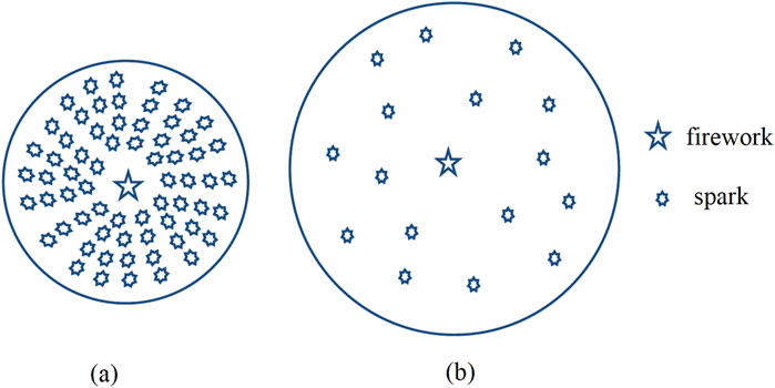
Figure 5. Fireworks explosion. (a) Good explosion. (b) Bad explosion.

3.3.1 Explosion amplitude and number of sparks

In our DFWA, the explosion amplitude and number of sparks associated with a firework (a feasible solution of formulation (1)–(14)) depends on its fitness (objective function value) through Formulas 15 and 16 (Tan, 2015; Tan and Zhu, 2010)

$n{s}_i=\widehat{M}\cdot \frac{ob{j}_{\mathit{worst}}-f\left(so{l}_i\right)+\xi }{{\sum }_{j=1}^N\left(ob{j}_{\mathit{worst}}-f\left(so{l}_j\right)\right)+\xi }(15)$

$A_i=⌈\widehat{A}\cdot \frac{f\left(so{l}_i\right)-ob{j}_{\mathit{best}}+\xi }{{\sum }_{j=1}^N\left(f\left(so{l}_j\right)-ob{j}_{\mathit{best}}\right)+\xi }⌉(16)$

where $so{l}_i$ refers to the $i$-th firework $(i=\mathrm{1,2},\dots ,N)$, $f(so{l}_i)$ represents its fitness, $\widehat{M}$ controls the number of sparks generated by each firework, $\widehat{A}$ denotes the maximum explosion amplitude, $\xi$ is a small constant that avoids division by zero errors, and $ob{j}_{\mathit{worst}}={\max }_{1\le j\le N}\{f(so{l}_j)\}$ and $ob{j}_{\mathit{best}}={\min }_{1\le j\le N}\{f(so{l}_j)\}$ are, respectively, the worst and best values of the objective function among the $N$ incumbent fireworks.

To avoid too many or too few sparks using Equation 15, an upper bound $\widehat{n{s}_i}$ on the number of sparks (Tan, 2015) is defined through (with $round()$ the rounding function)

$\widehat{n{s}_i}=\left\{\begin{array}{cc}round\left(a\times \widehat{M}\right),\hfill & \text{if\hspace{0.17em}}n{s}_i<a\times \widehat{M}\hfill \\ round\left(b\times \widehat{M}\right),\hfill & \text{if\hspace{0.17em}}n{s}_i>b\times \widehat{M}\text{,\hspace{0.17em}}a<b<1\hfill \\ round\left(n{s}_i\right),\hfill & \text{otherwise}\hfill \end{array}\right.(17)$

for properly chosen constants $a$ and $b$.

3.3.2 Generation of sparks

Our algorithm generates a spark from $so{l}_i$ through the swap move. We use a simple swap by randomly selecting two sites and swapping the corresponding elements. This is repeated $A_i$ times.

As mentioned, good sparks suggest closeness to an optimal or near-optimal solution. Thus, the explosion process should preserve features of good solutions, and hence only the best-fit spark is selected from the $A_i$ swapped solutions. One spark can be obtained from each swap move, and $\widehat{n{s}_i}$ sparks are generated thereafter, iteratively carrying out $A_i\ast \widehat{n{s}_i}$ swap moves. Note that the iterative swap move used in the explosion operator essentially entails a local search to generate relatively better sparks, possibly improving the performance of our DFWA. Figure 6 illustrates the generation of a spark with $A_i=4$. Pseudo-code for generating one spark is available in Algorithm 2, whereas Algorithm 3 details pseudo-code for the explosion procedure called by Algorithm 1.

Figure 6

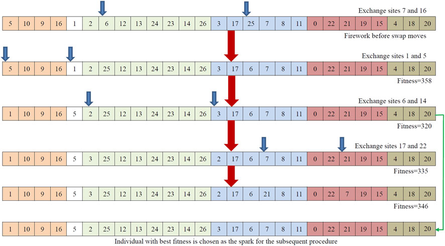
Figure 6. Illustration of spark generation with $A_i=4$.

Algorithm 2

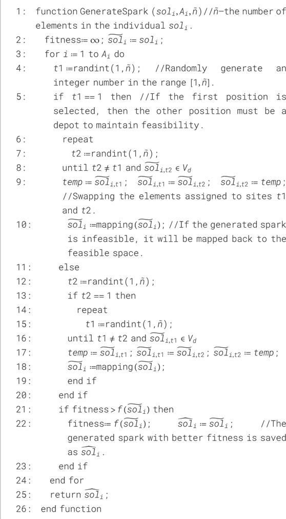
Algorithm 2. Pseudo-code to generate one spark.

Algorithm 3

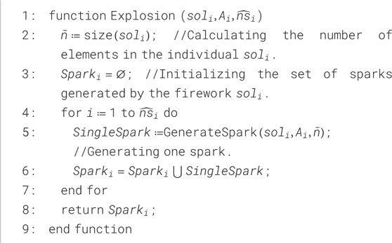
Algorithm 3. Explosion procedure pseudo-code.

Recall that once a move is executed, the new solution might need to be recodified to ensure its feasibility. For example, if the first position is selected for a swap, it should be replaced by another depot.

3.4 Mutation operator

As with other swarm intelligence algorithms, maintaining population diversity is crucial for the efficiency of the DFWA to promote full exploration of the most interesting regions of the search space. Mutation is a major diversification technique employed within swarm heuristic algorithms. It refers to the process of increasing population diversity to mitigate stagnation in unpromising areas and promote the exploration of new search regions by introducing random variations in the individual solutions (Zhang et al., 2022b). In this study, the mutation operator is implemented through two search mechanisms—insertion and inversion moves—which are chosen with equal probabilities. Algorithm 4 presents pseudo-code for the mutation procedure.

Algorithm 4

Algorithm 4. Pseudo-code for the mutation procedure.

3.4.1 Insertion move

This move randomly selects the $i$-th and $j$-th positions ($i\ne 1$ and $i<j$) from a solution permutation and then inserts the element in the $i$-th position in front of the element in the $j$-th position. Figure 7 and Algorithm 5 show an illustration and pseudo-code of the insertion move, respectively.

Figure 7

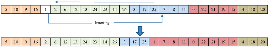
Figure 7. Illustration of insertion move.

Algorithm 5

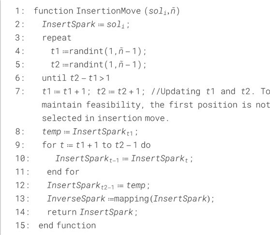
Algorithm 5. Pseudo code for insertion move.

Algorithm 6

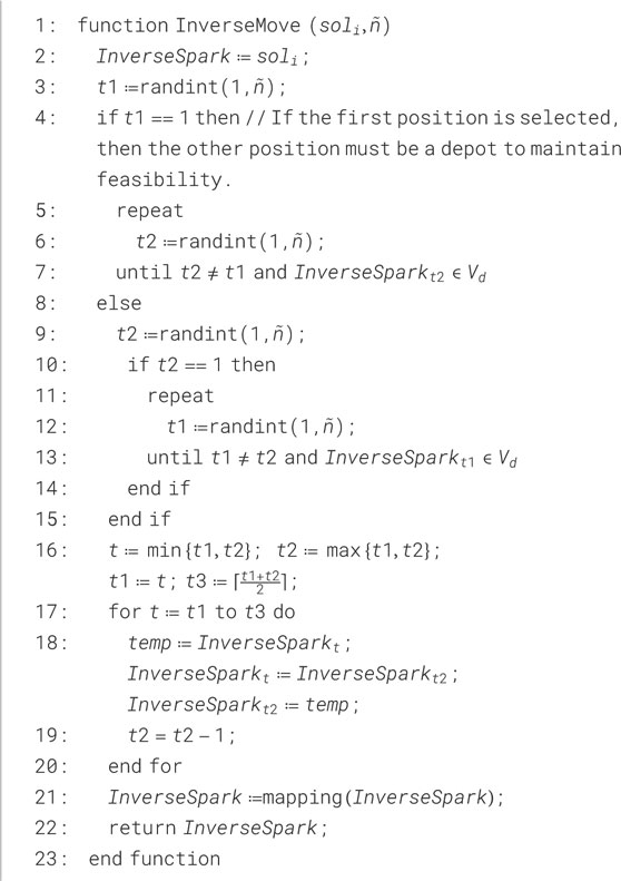
Algorithm 6. Pseudo code for inversion move.

3.4.2 Inversion move

Inversion move. This move randomly selects the $i$-th and $j$-th positions ($i\ne 1$ and $i<j$) from a solution permutation and then inverts the sub-permutation between both positions. Figure 8 and Algorithm 6 illustrate the inversion move and its pseudo-code, respectively.

Figure 8

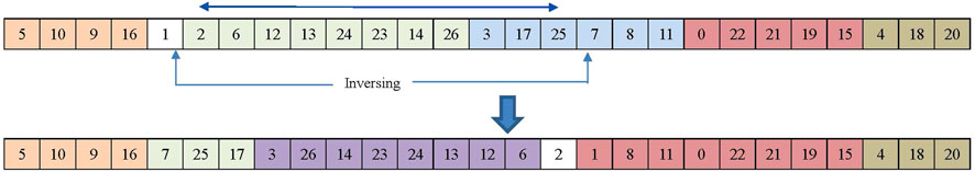
Figure 8. Illustration of inversion move.

3.5 Mapping rule

Some of the generated sparks using the swap move and mutation procedures could be infeasible, and they should be mapped back to the feasible region. Indeed, if a spark generated by a move is infeasible, at least one of the following two cases holds.

Case 1. The resulting customers’ demand assigned to the $i$-th depot exceeds its capacity. In this case, a customer is randomly selected from the set $Cusd(i)$ of customers allocated to depot $i$ and assigned to a randomly selected open depot $j$, the remaining capacity of which can satisfy the demand of the selected customer. If no open depot can satisfy the selected customer, a closed depot is randomly selected to serve such customer. This procedure is repeatedly carried out until all open depots may satisfy their customers’ demand.

Case 2. The resulting customers’ demand served by the $k$-th vehicle exceeds its capacity. In this case, a customer is randomly selected from the set $Cusv(k)$ of customers served by the $k$-th vehicle and assigned to a randomly selected vehicle starting at the same depot as vehicle $k$, with remaining capacity available to satisfy the selected customer’s demand. If no such vehicle exists, a new vehicle will be launched in the same parking lot as vehicle $k$ to serve the selected customers. This procedure is repeated until all vehicles may satisfy the demands of the customers they serve.

Algorithm 7 presents pseudo-code for dealing with both cases. The random selection mechanism in the mapping rule ensures simplicity and avoids excessive computation for small-to-medium OCLRP instances but may lead to inefficiencies in large-scale cases (e.g., 100+ customers or 10+ depots). Repeated random selections can result in redundant reallocations, such as frequently reassigning small-demand customers or choosing depots and vehicles with minimal residual capacity, thus increasing the need for additional repair steps. To address this issue, two optimized strategies are proposed for future implementation while preserving the core logic of the mapping rule:

1. Residual capacity-greedy selection: for depot-level capacity violations (Case 1), prioritize reallocating the customer with the highest demand from the overloaded depot to an open depot with the largest available capacity; for vehicle-level violations (Case 2), assign the largest-demand customer to the vehicle within the same depot that has the maximum residual capacity.

2. Distance-aware selection: when reallocating, combine residual capacity with routing distance by selecting the depot or vehicle that offers sufficient capacity and the smallest additional travel distance (either from the customer or from the last customer in the vehicle’s current route).

It is worth noting that the current random selection plays a crucial role in maintaining population diversity in DFWA, thus helping avoid premature convergence to local optima. For large-scale problems, a hybrid approach (e.g., 80% greedy selection and 20% random selection) could potentially balance computational efficiency and solution diversity. However, such an approach would require further parameter tuning and validation using large-scale benchmarks (e.g., instances with 200+ customers); this is reserved for future research to avoid complicating the current DFWA framework.

Algorithm 7

Algorithm 7. Pseudo-code of the mapping rule.

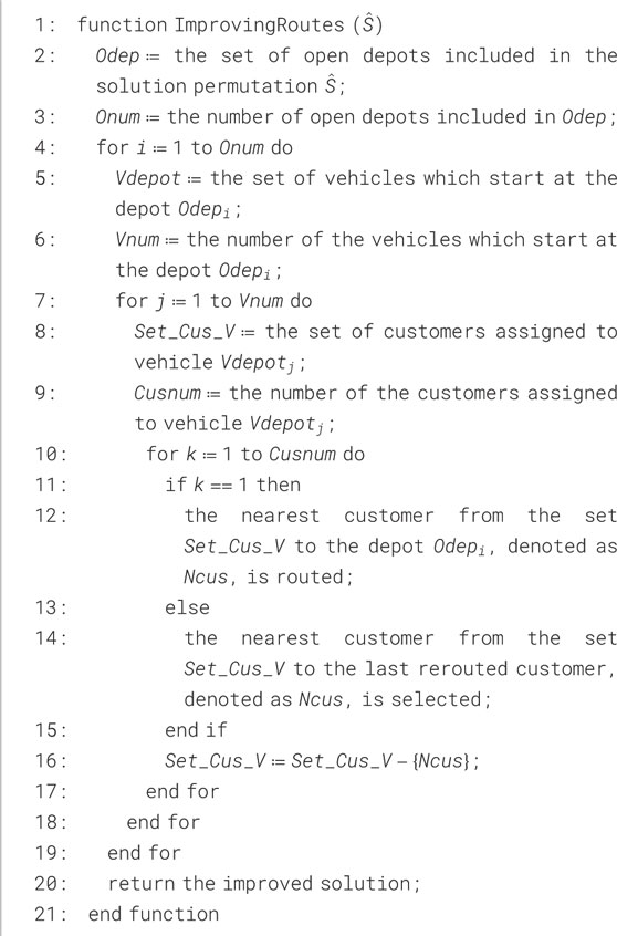
3.6 Improving the routes

For each solution generated using the explosion and mutation operators, the distribution routes included in it are improved using a greedy search method. The customers assigned to the same distribution route may be rerouted in this step. First, for each route, the customer nearest the depot which provides service to it is routed. Next, the customer nearest the last rerouted is selected. This is repeated until all customers assigned to the current vehicle are rerouted. Algorithm 8 presents pseudo-code to improve the distribution routes.

Algorithm 8

Algorithm 8. Pseudo-code to improve routes.

3.7 Selection strategy

Based on the explosion and mutation sparks and the current fireworks, $N$ solutions are selected to form the next generation of fireworks. The selection uses a fitness-and-Hamming-distance-based strategy aimed at promoting good solution features as well as diversity.

Prior to calculating the Hamming distance, each candidate $so{l}_i$ is rewritten as ${\widetilde{sol}}_i$, encoded through the depots’ indices and including $m+n$ elements. In ${\widetilde{sol}}_i$, the $m$ depots (numbered 1 to $m$) are placed in the first $m$ positions in order, with the element ${\widetilde{sol}}_{ij}$ $(j>m)$ representing the depot to which the $j$-th customer is allocated. Figure 9 illustrates the transformation from $so{l}_i$ to ${\widetilde{sol}}_i$. In it, customers 10, 9, and 16 are allocated to depot 5 in $so{l}_i$. Thus, the ${\widetilde{sol}}_i$ elements located in positions 10, 9, and 16 are five. Then, for each solution $so{l}_i$, an index $R(so{l}_i)$ is computed defined as the sum of Hamming distances from $so{l}_i$ to the other individuals, computed through

$R\left(so{l}_i\right)={\displaystyle \sum _{j\in \mathcal{F},j\ne i}}Dis\left(so{l}_i,so{l}_j\right)={\displaystyle \sum _{j\in \mathcal{F},j\ne i}}Dis\left({\widetilde{sol}}_i,{\widetilde{sol}}_j\right),(18)$

where $Dis(so{l}_i,so{l}_j)$ is the Hamming distance between $so{l}_i$ and $so{l}_j$ (the Hamming distance between two permutations is the number of positions at which the corresponding elements are different) and $\mathcal{F}$ denotes the set of candidate solutions (consistent with the notation in line 21 of Algorithm 1 and line 1 of Algorithm 9).

Figure 9

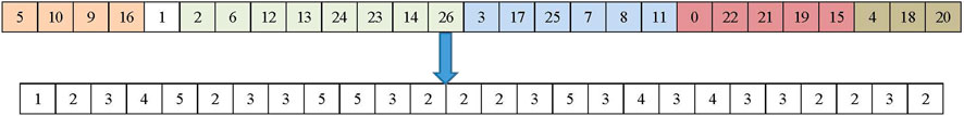
Figure 9. Transformation from $so{l}_i$ to ${\widetilde{sol}}_i$.

Our implementation passes down the individual with the best fitness value down to the next generation. The remaining $N-1$ next-generation individuals are selected using the roulette wheel principle, with probability $Pro(so{l}_i)$ of choosing the individual $so{l}_i$ computed through Formula 19:

$Pro\left(so{l}_i\right)=\frac{\frac{1}{{\left(f\left(so{l}_i\right)\right)}^2}+R\left(so{l}_i\right)}{{\sum }_{i\in \mathcal{F}}\frac{1}{{\left(f\left(so{l}_i\right)\right)}^2}+{\sum }_{i\in \mathcal{F}}R\left(so{l}_i\right)}(19)$

From Equation 19, observe that individuals with larger distances and better fitness will have more chances of being passed on to the next generation. Thus, this selection strategy promotes both the good characteristics and diversity of the population. In Equation 19, the quadratic power increases the probability of selecting good individuals compared to the first power. Algorithm 9 presents the pseudo-code implementing the selection strategy.

Algorithm 9

Algorithm 9. Pseudo-code to select next-generation fireworks.

4 Computational analysis

This section reports extensive computational experiments undertaken to assess the performance of the DFWA proposed to solve OCLRPs. For reasons outlined above, we use the data of benchmark CLRP instances without any adjustment to test our algorithm. Implementation is based on Matlab R2016a, and experiments were conducted on a laptop equipped with an A10-7400P CPU at 3.40 GHz and 4 GB of RAM under Windows 10.

4.1 Parameter setting and sensitivity analysis

It is well-known that the proper tuning of parameters may considerably affect the performance of most meta-heuristic algorithms (Zhang et al., 2022a). In our DFWA case, we carried out experiments with two randomly selected benchmark instances—Gaskell67-21×5 and Gaskell67-29×5 (Yu and Lin, 2015) —averaged over 20 independent runs over each instance, using the average gap with respect to the best known solution, the average computing time, and the average number of runs to reach the best solution depending on the following key parameters: number of fireworks, parameter controlling the number of explosion sparks, maximum explosion amplitude, and number of mutation sparks. Only one parameter was modified at a time.

4.1.1 Number of fireworks

To properly set the number of fireworks, we investigated six different values (0.5, 1, 1.5, 2, 2.5, 3) as multipliers of the number $n+m$ of customers and depots in the instance (i.e., 0.5$(n+m)$, $n+m$, ….). Table 1 presents, for each number of fireworks, average results over the 20 runs for both instances for the percent deviation from the best-known solution $(\mathrm{G}\mathrm{a}{\mathrm{p}}_{\mathrm{a}\mathrm{v}\mathrm{e}}=\frac{\mathrm{B}\mathrm{O}{\mathrm{V}}_{\mathrm{a}\mathrm{v}\mathrm{e}}-\mathrm{B}\mathrm{K}\mathrm{O}\mathrm{V}}{\mathrm{B}\mathrm{K}\mathrm{O}\mathrm{V}}\times 100\%)$, where $\mathrm{B}\mathrm{O}{\mathrm{V}}_{\mathrm{a}\mathrm{v}\mathrm{e}}$ is the average objective value over 20 runs and $\mathrm{B}\mathrm{K}\mathrm{O}\mathrm{V}$ is the best-known objective value reported in the literature, the average computing time in seconds, and the number of runs until generating the best solution.

Table 1

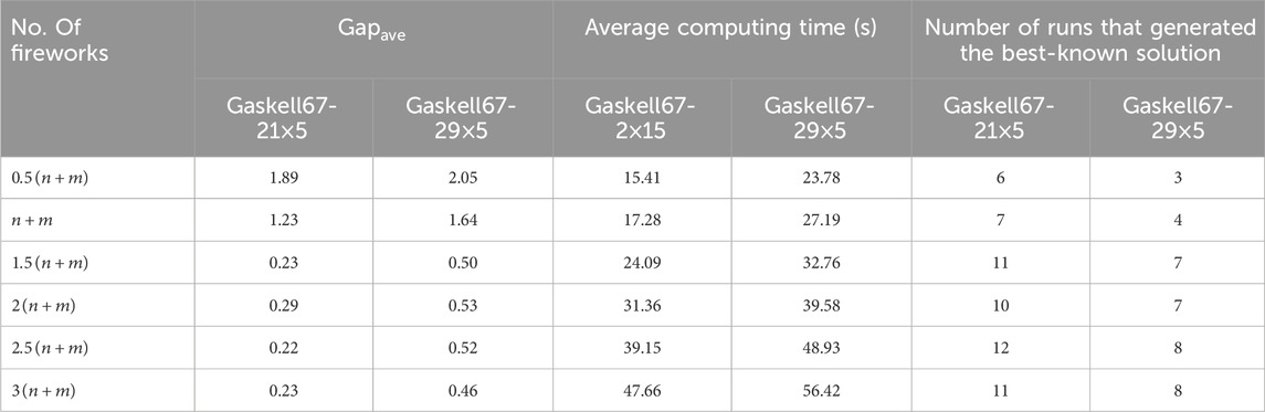
Table 1. Average results with different number of fireworks for Gaskell67-21×5 and Gaskell67-29×5.

According to this table, the number of fireworks plays a key role in the performance of our DFWA. When a small number is employed (like 0.5$(n+m)$), the algorithm tends to end up in a local optimum, with a worse average objective value and a smaller number of runs. On the other hand, for large numbers of fireworks (like 3$(n+m)$), better average results are attained, albeit at much longer computational times. Based on the solution quality and computing time, we would suggest using $N=1.5(n+m)$, $2(n+m)$, or $2.5(n+m)$ fireworks in our framework.

4.1.2 Parameter $\widehat{M}$

The number of explosion sparks is also a crucial parameter in searching for good solutions. A small number of explosion sparks might not strengthen exploration in a promising search region, decreasing the possibility of obtaining the optimal solution. However, a larger number of explosion sparks typically ends up being very similar to an exhaustive method, greatly increasing computing time. Table 2 presents average results over 20 runs for both instances using different values of $\widehat{M}$ which controls the number of sparks generated by a firework as a multiple of the number $N$ of fireworks, from $0.5N$ to $3N$. This table suggests that better values for $\widehat{M}$ in our experiments are $1.5N$, $2N$, and $2.5N$, based on the number of runs and the values of $\mathrm{G}\mathrm{a}{\mathrm{p}}_{\mathrm{a}\mathrm{v}\mathrm{e}}$.

Table 2

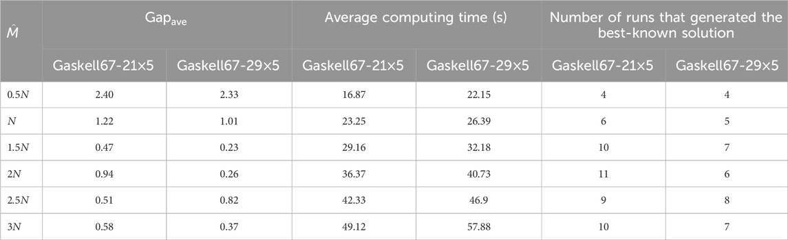
Table 2. Average results using different values of $\widehat{M}$ for Gaskell67-21×5 and Gaskell67-29×5.

4.1.3 Number of mutation sparks

For the proposed DFWA, properly balancing exploration and exploitation critically depends on choosing a suitable number of mutation sparks. A small number hinders the procurement of the optimal solution as the entailed lower population diversity interferes with escaping from a local optimum toward novel unexplored areas. However, a larger number of mutation sparks resembles a naive random multi-start approach. To select a suitable number of mutation sparks, six different multiples of $(n+m)$ were considered. Table 3 presents average results over 20 runs for both test instances, depending on the number of mutation sparks. Comparatively better number of runs and optimality gaps were globally obtained with $n+m$ and $1.5(n+m)$.

Table 3

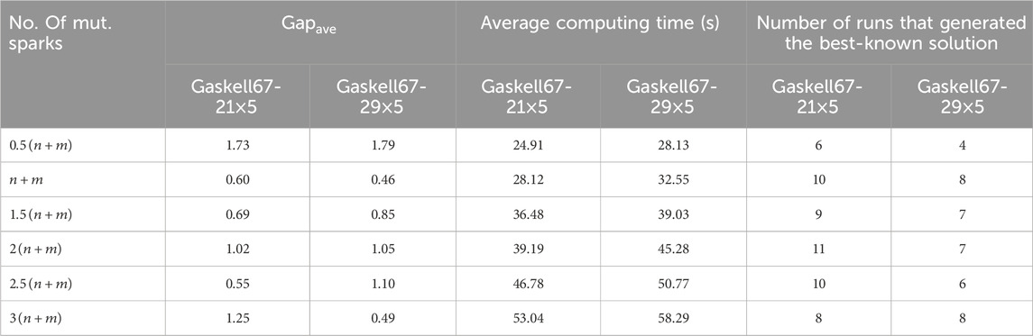
Table 3. Average results using different number of mutation sparks for Gaskell67-21×5 and Gaskell67-29×5.

4.1.4 Parameter $\widehat{A}$

In our algorithm, this parameter denotes the maximum swap moves for generating one explosion spark. When $\widehat{A}$ is small, the sparks generated using swap moves cannot be sufficiently improved; however, when $\widehat{A}$ is too large, it is also possible to become trapped in meaningless iterations. To properly set $\widehat{A}$, six values are considered (as multiples of $N$). Table 4 presents average results over 20 runs for our test instances. Comparatively better values of $\widehat{A}$ are obtained in our experiments with $1.5N$ and $2N$ based on the relatively better average number of runs and value of $\mathrm{G}\mathrm{a}{\mathrm{p}}_{\mathrm{a}\mathrm{v}\mathrm{e}}$.

Table 4

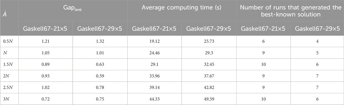
Table 4. Average results using different values of $\widehat{A}$ for Gaskell67-21×5 and Gaskell67-29×5.

4.1.5 Parameter combinations

We undertook additional experiments to identify good parameter combinations. Table 5 lists the 36 combinations tested, based on those found above, for which ten runs over our two selected Gaskell instances took place.

Table 5

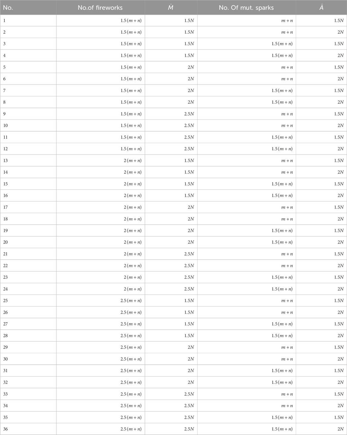
Table 5. Parameter combinations.

Table 6 presents the average results for each parameter combination.

Table 6

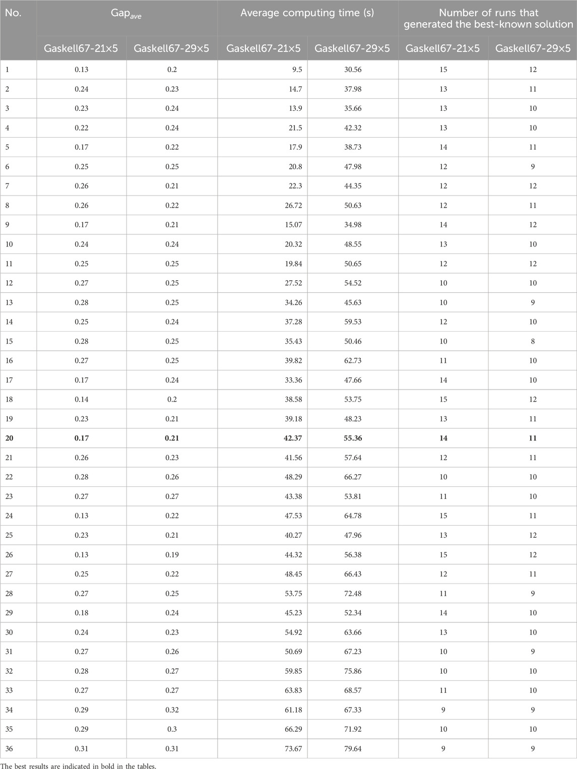
Table 6. Results for parameter combinations.

A closer look at Table 6 reveals that combination 26 shows marginal advantages in solution quality and success rate—its ${\text{Gap}}_{\mathit{ave}}$ for Gaskell67-21$\times$5 and Gaskell67-29$\times$5 is 0.13% and 0.19% (slightly lower than combination 20s 0.17% and 0.21%), and the number of runs generating the best-known solution is 15 and 12 (same as combination 20s 14 and 11). However, combination 20, associated with parameter choices $2(m+n)$, $2N$, $1.5(m+n)$, and $2N$, was ultimately selected as the optimal parameter set, the rationale lying in the balance between computational efficiency and solution quality, especially considering practical application scenarios. For the two test instances, combination 20 exhibits slightly shorter computation time than combination 26: 42.37 s vs. 44.32 s for Gaskell67-21$\times$5 ($\approx$2-s difference) and 55.36 s vs. 56.38 s for Gaskell67-29$\times$5 ($\approx$1-s difference). While this time gap seems minimal in a single run, it accumulates significantly when the algorithm is executed repeatedly—for example, in large-scale benchmark testing (e.g., 10,000 runs for 33 OCLRP instances in Section 4.3) or real-world dynamic logistics scenarios (e.g., daily route optimization for a company with 100+ delivery points), the total time saved by combination 20 would be approximately 10,000$\times$(2 + 1)/2 = 15,000 s ($\approx$4.2 h) for the two instances alone. For larger instances (e.g., 100-5-1 with 100 customers), this cumulative advantage would be even more pronounced, as computation time scales with problem size.

In all these preliminary experiments, the best solution obtained by the proposed DFWA could not be further improved after 400 iterations where we had included a maximum number $G=500$ of iterations and a termination condition for the search process if the best solution thus far found could not be improved after 100 iterations.

4.2 Comparative performance

As described, our DFWA was initially based on a greedy initialization and iterated swap, insertion, and inverse moves respectively employed to generate good initial solutions, strengthen local search, and enhance population diversity. To further investigate the effectiveness of the proposed search strategies, we compared it with four alternative DFWAs by solving eight representative OCLRP instances (small-scall: Gaskell67-21$\times$5, Gaskell67-22$\times$5, Gaskell67-$29\times 5.$ medium-scale: 50-5-1, 50-5-3b. large-scale: 100-5-1, 100-10-1, 100-10-3b) systematically selected from 33 benchmark instances (Tables 7 and 8). These instances cover different scales and customer/depot ratios to ensure generalizability. The alternative algorithms were as follows

Table 7

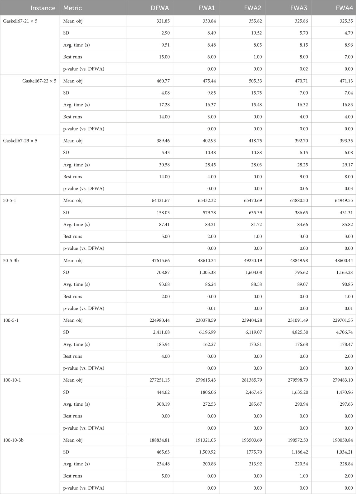
Table 7. Comparison among DFWA, FWA1, FWA2, FWA3, and FWA4.

Table 8

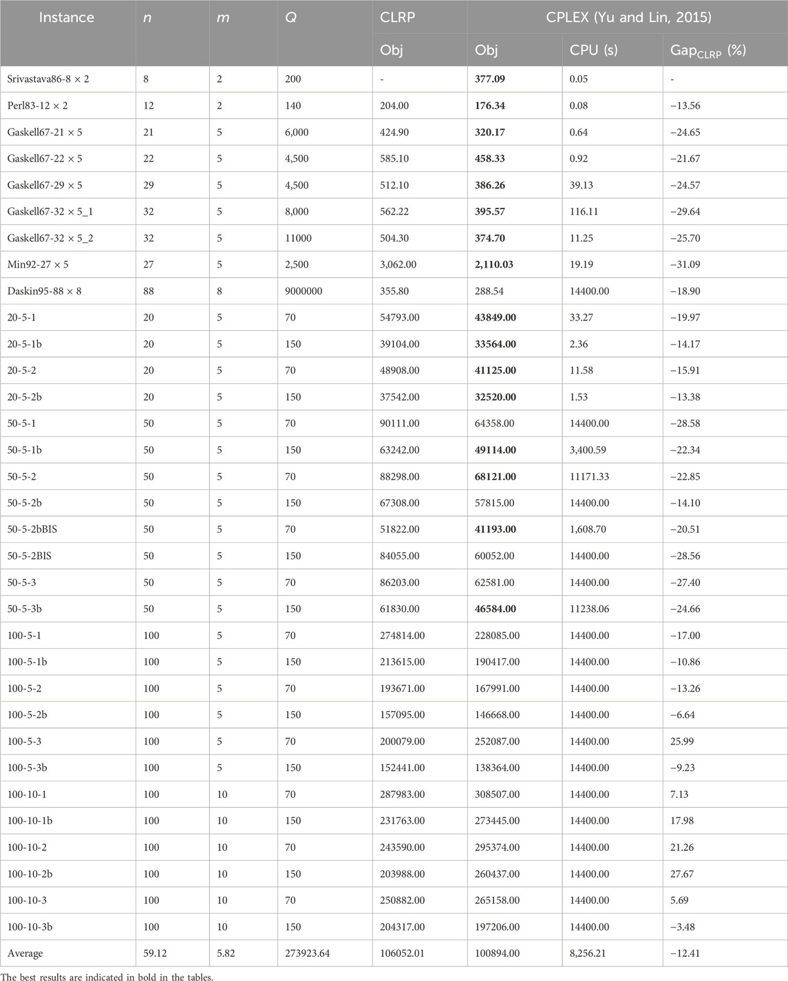
Table 8. Comparison of results with the OCLRP solved with CPLEX and best-known results of corresponding CLRP.

FWA1: initial solution is randomly generated rather than through greedy search. This serves to evaluate whether the proposed greedy approach enhances the overall performance of the DFWA.

FWA2: proposed DFWA except for the iterated swap move imitates the explosion operator, which is removed. This serves to assess the effectiveness of such a move.

FWA3: proposed DFWA except for the insertion move, which is dropped. This serves to assess the effectiveness of the insertion move.

FWA4: proposed DFWA without inverse move, which is therefore assessed.

To ensure a fair comparison, all four alternative algorithms (FWA1–FWA4) adopt the same parameter combination as the original DFWA. No separate parameter tuning was performed for FWA1–FWA4; this eliminates the interference of parameter differences on performance and ensures that any observed gaps in results are attributed to the absence of specific components (greedy initialization, swap/insertion/inverse moves) rather than parameter adjustments.

Table 7 reports the comprehensive performance metrics of the five algorithms over 20 independent runs per instance, including mean objective value, standard deviation (SD) of objective value, average computation time (s), number of runs that found the best-known solution, and p-values (vs. DFWA from Wilcoxon signed-rank test). Except for the instance Gaskell67-$29\times 5$, in which the p-value for the comparison between FWA3 and DFWA is larger than 0.05, all other p-values were less than 0.05, indicating statistically significant differences among FWA1–FWA4 and DFWA. Table 7 clearly shows that DFWA outperforms the other four algorithms in all instances in terms of both statistics. FWA2 provides the worst mean and SD; additionally, pairwise differences between the original DFWA and the four modifications seem significant according to the boxplots in Figure 10. Table 7 also suggests that: (1) the combination of the insertion and inversion move not only effectively improves DFWA population diversity, allowing it to escape from a current local optimum and move to non-previously visited spaces, but also enhances the exploration capabilities of the algorithm; (2) besides effectively strengthening the local search of the DFWA, the iterated swap move also enhances the exploitation capabilities of the DFWA; (3) the greedy approach tends to generate a relatively good-quality initial population, playing a significant role in improving the DFWA performance. To sum up, DFWA achieves better performance than FWA1–FWA4.

Figure 10

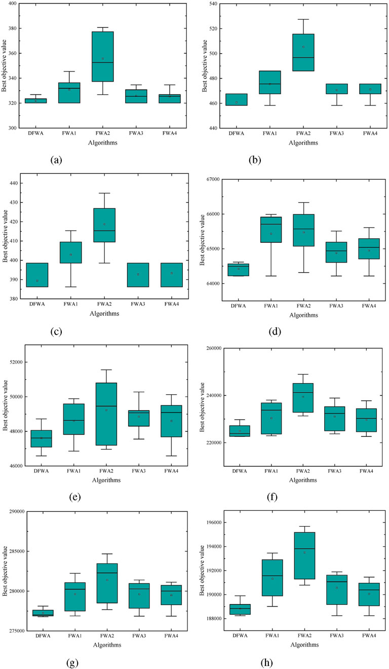
Figure 10. Box plots of DFWA, FWA1, FWA2, FWA3, and FWA4 on four small instances. (a) Gaskell67-21 × 5. (b) Gaskell67-22 × 5. (c) Gaskell67-29 × 5. (d) 50-5-1. (e) 50-5-3b. (f) 100-5-1. (g) 100-10-1. (h) 100-10-3b.

Moreover, Table 7 also suggests that DFWA seems more stable than the four variants, as also reported through the box plots in Figure 10 portraying the results of the five FWAs on eight instances.

4.3 Benchmarking our DFWA

To assess the performance of our DFWA in solving OCLRPs, we obtained 33 instances from the corresponding CLRP benchmark instances, solved them, and compared their results with those in Yu and Lin (2015) and their best-known solution.

Table 8 presents the benchmark results obtained by solving the OCLRP with CPLEX and the best-known CLRP solution. Each row provides the number $n$ of customers, the number $m$ of depots, the capacity $Q$ of each depot, the best known objective value of the CLRP instance (from Ting and Chen, 2013), the best objective value obtained with CPLEX (from Yu and Lin, 2015), the CPU seconds spent by CPLEX, and the percent deviation from the best-known CLRP solution $(\mathrm{G}\mathrm{a}{\mathrm{p}}_{\mathrm{C}\mathrm{L}\mathrm{R}\mathrm{P}}=\frac{\mathrm{O}\mathrm{b}\mathrm{j}.\mathrm{o}\mathrm{b}\mathrm{t}\mathrm{a}\mathrm{i}\mathrm{n}\mathrm{e}\mathrm{d}\mathrm{u}\mathrm{s}\mathrm{i}\mathrm{n}\mathrm{g}\mathrm{C}\mathrm{P}\mathrm{L}\mathrm{E}\mathrm{X}-\mathrm{O}\mathrm{b}\mathrm{j}.\mathrm{o}\mathrm{f}\mathrm{C}\mathrm{L}\mathrm{R}\mathrm{P}}{\mathrm{O}\mathrm{b}\mathrm{j}.\mathrm{o}\mathrm{f}\mathrm{C}\mathrm{L}\mathrm{R}\mathrm{P}}\times \mathrm{100}\mathrm{\%})$. The last row provides average values. Values in bold indicate that the optimal solution is obtained within 14,400 s for each instance. Yu and Lin (2015) used CPLEX 12.0 and a simulated annealing heuristic implemented in Microsoft Visual C++ 2008 to solve the OCLRP instances on a laptop equipped with A10-7400P CPU at 3.40 GHz and 4 GB of RAM under Windows 10. These are key parameters in the SA (Yu and Lin, 2015): the iteration number equals $5000L$, where $L$ is the coding length of the solution representation; the maximum allowable number of consecutive temperature reductions without improvement in the solution value is 100; the initial temperature is 30, and the final temperature is 0.1; the Boltzmann constant used in calculating the probability of accepting a worse solution is 1/9; the coefficient of the cooling schedule is 0.99.

Some might question whether the objective function values between the CLRP and OCLRP are comparable. After all, the OCLRP vehicle costs should differ from those in the CLRP, since the vehicles in the OCLRP are leased and are thus not owned by the company. However, the objective values in Table 8 are only used to explain that the logistics costs of the OCLRP are lower than those of the CLRP when vehicle costs are the same. In reality, should the logistics costs of the TPL company be lower than the logistics cost of the company’s own distribution, the company would outsource its logistics activities to the TPL provider. Otherwise, the company would not outsource such activities. This provides a decision-support argument in relation to outsourcing logistics.

As Table 8 shows, CPLEX finds feasible solutions for all 33 instances, with 16 of them optimally solved within 14,400 s. However, the computing time grows considerably with instance size. For 26 out of 33 test instances, CPLEX provided lower objective values than the corresponding CLRP instances. Such value difference could suggest potential benefits of outsourcing logistics (Yu and Lin, 2015). In particular, we can observe that the percentage deviation from the best-known objective value of the CLRP varies from −13.38% to −31.09%, indicating that the OCLRP can save important costs by outsourcing logistics (about 19.33% for the above-mentioned 26 instances).

Table 9 compares the results attained over the 33 OCLRP instances with our DFWA and SA—a powerful state-of-the-art heuristic algorithm for solving the OCLRP (Yu and Lin, 2015). As mentioned, the OCLRP has been significantly less investigated in the literature. Thus, we only compare the proposed algorithm with a heuristic in our study, as it is difficult to find other heuristic algorithms used to solve the OCLRP. Besides the objective value (Obj.) and CPU time spent by both algorithms, the table also provides the percentage deviation from the best-known solution of the CLRP $(\mathrm{G}\mathrm{a}{\mathrm{p}}_{\mathrm{C}\mathrm{L}\mathrm{R}\mathrm{P}})$ and the percentage deviation from the best solution obtained with CPLEX $(\mathrm{G}\mathrm{a}{\mathrm{p}}_{\mathrm{C}\mathrm{P}\mathrm{L}\mathrm{E}\mathrm{X}}=\frac{\mathrm{O}\mathrm{b}\mathrm{j}.\mathrm{o}\mathrm{b}\mathrm{t}\mathrm{a}\mathrm{i}\mathrm{n}\mathrm{e}\mathrm{d}\mathrm{u}\mathrm{s}\mathrm{i}\mathrm{n}\mathrm{g}\mathrm{S}\mathrm{A}(\mathrm{o}\mathrm{r}\mathrm{D}\mathrm{F}\mathrm{W}\mathrm{A})-\mathrm{O}\mathrm{b}\mathrm{j}.\mathrm{o}\mathrm{b}\mathrm{t}\mathrm{a}\mathrm{i}\mathrm{n}\mathrm{e}\mathrm{d}\mathrm{u}\mathrm{s}\mathrm{i}\mathrm{n}\mathrm{g}\mathrm{C}\mathrm{P}\mathrm{L}\mathrm{E}\mathrm{X}}{\mathrm{O}\mathrm{b}\mathrm{j}.\mathrm{o}\mathrm{b}\mathrm{t}\mathrm{a}\mathrm{i}\mathrm{n}\mathrm{e}\mathrm{d}\mathrm{u}\mathrm{s}\mathrm{i}\mathrm{n}\mathrm{g}\mathrm{C}\mathrm{P}\mathrm{L}\mathrm{E}\mathrm{X}}\times \mathrm{100}\mathrm{\%})$. Values in bold indicate the best result between both algorithms. Note that the best objective values obtained using SA are calculated using the distribution routes found in Yu and Lin (2015).

Table 9

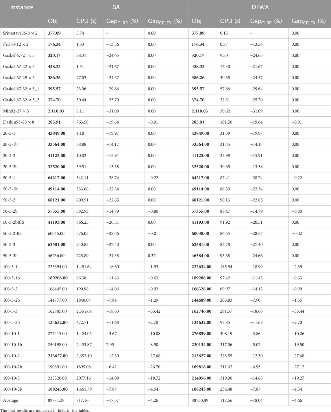
Table 9. Comparison between simulated annealing and the proposed DFWA.

From Table 9, we appreciate that SA and DFWA obtained the same results in 23 instances, whereas DFWA produced better solutions (and lower percentage deviations) in the remaining ten. Moreover, the average percentage deviations ($\mathrm{G}\mathrm{a}{\mathrm{p}}_{\mathrm{C}\mathrm{P}\mathrm{L}\mathrm{E}\mathrm{X}}$ and $\mathrm{G}\mathrm{a}{\mathrm{p}}_{\mathrm{C}\mathrm{L}\mathrm{R}\mathrm{P}}$) produced by DFWA over the 33 instances are lower than the corresponding values generated by SA. Thus, the proposed DFWA slightly outperforms SA in terms of solution quality. Concerning CPU times, we observe that, except for instances Gaskell67-$22\times 5$, Gaskell67-$32\times 5$_1, Min92-$27\times 5$, 20-5-1, 20-5-2, and 100-5-1b, the DFWA spent far less computational time in solving the instances. Note that different hardware, compilers, and programming languages could have a significant impact on the comparison. For our proposed DFWA, the slower MATLAB code did not seem to result in very large computational times.

Moreover, the results presented in Tables 7 and 8 enable a comparison between our DFWA and the CPLEX implementation. DFWA provides the same or better solutions. On the other hand, CPLEX spent slightly less computational time than our DFWA in most instances, with the number of customers smaller than 32. However, for instances with 50 or more customers, CPLEX spent much more computational time, and our DFWA provides better solutions within less than 330 s. The average computational time spent by CPLEX is about 8,256.21 s—much longer than DFWA’s average 117.56 s. Thus, compared to CPLEX and SA, our DFWA seems to provide good solutions in a reasonable time for large-size OCLRP instances.

We also performed non-parametric Friedman and Wilcoxon signed-rank tests (at a significance level 0.05) to assess the statistical significance of the observed differences between DFWA and SA based on the $\mathrm{G}\mathrm{a}{\mathrm{p}}_{\mathrm{C}\mathrm{P}\mathrm{L}\mathrm{E}\mathrm{X}}$ in Table 9. The average ranks for the Friedman test are 1.35 and 1.65, respectively, for the DFWA and SA, and the corresponding Friedman ${\chi }_F^2$ statistic and $p$-value are 10 (critical value is 3.84) and 0.002. This suggests a rejection of the null hypothesis and indicates a significant difference between DFWA and SA results. Similarly, the Wilcoxon signed-ranks non-parametric test was applied to detect differences between DFWA and SA at instance level (pairwise comparison). The $p$-value was 0.005, suggesting the rejection of the null hypothesis and, again, statistical differences between our DFWA and the compared SA. Hence, the proposed algorithm seems truly competitive when solving OCLRPs.

4.4 A real case

Given the successful benchmarking of our DFWA for OCLRP, we tested it in a real case for a company that delivers to fruit and vegetable supermarkets in Shanghai, China. This company has been using five 12-ton capacity vehicles for daily distribution of merchandise from two depots to 16 supermarkets in the city. The transportation and monthly fixed costs (including only monthly depreciation) are, respectively, 5 Yuan per kilometer and 1,000 Yuan. Table 10 presents the current five distribution routes and monthly delivery costs (covering routing, fixed vehicle, depot rental costs). Depots are numbered 1 to 4 (the current two, plus an additional two), with their features in Table 11, and supermarkets are numbered 5 to 20.

Table 10

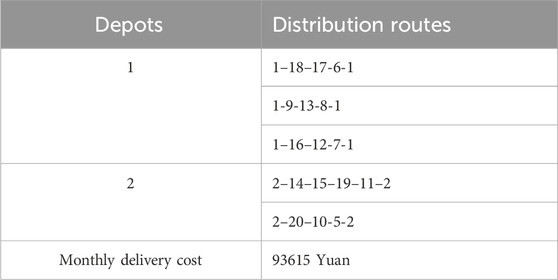
Table 10. Current distribution routes and delivery costs.

Table 11

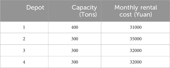
Table 11. Capacities and rental costs of four potential depots.

In order to strengthen its competitive ability and save distribution costs, this company considers optimizing its logistics system. Besides the two current depots, two additional potential depots numbered 3 and 4 are contemplated. Figure 11 illustrates the locations of the depots and the supermarkets. Table 12 shows the daily demand of these. Table 13 lists the distances between each pair of points. The company needs to determine which depots from the four candidates should be open to provide service to the 16 supermarkets and whether it should outsource its delivery activities to a TPL company.

Figure 11

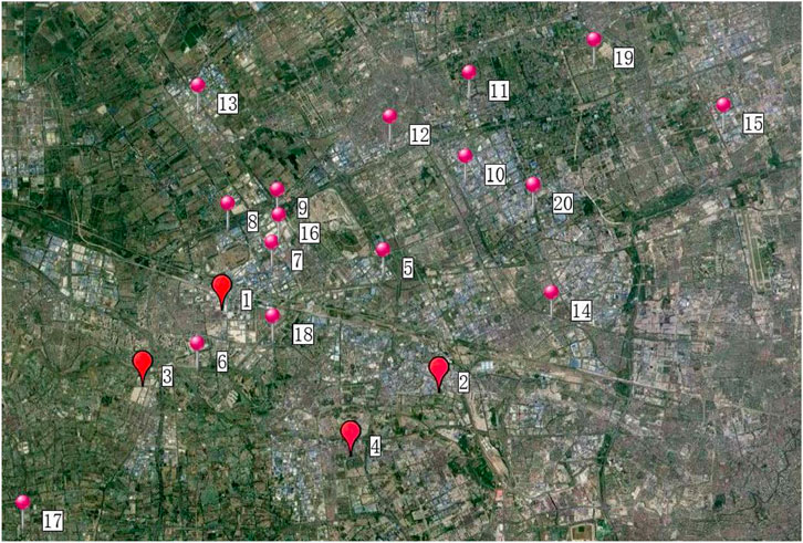
Figure 11. Map with four potential depots (1–4) and 16 delivery points (5–20) (supermarkets).

Table 12

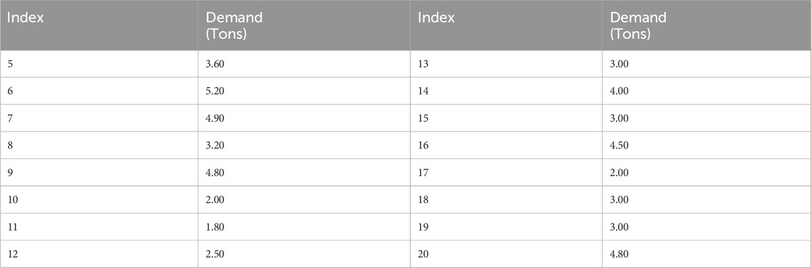
Table 12. Demand at each delivery point.

Table 13

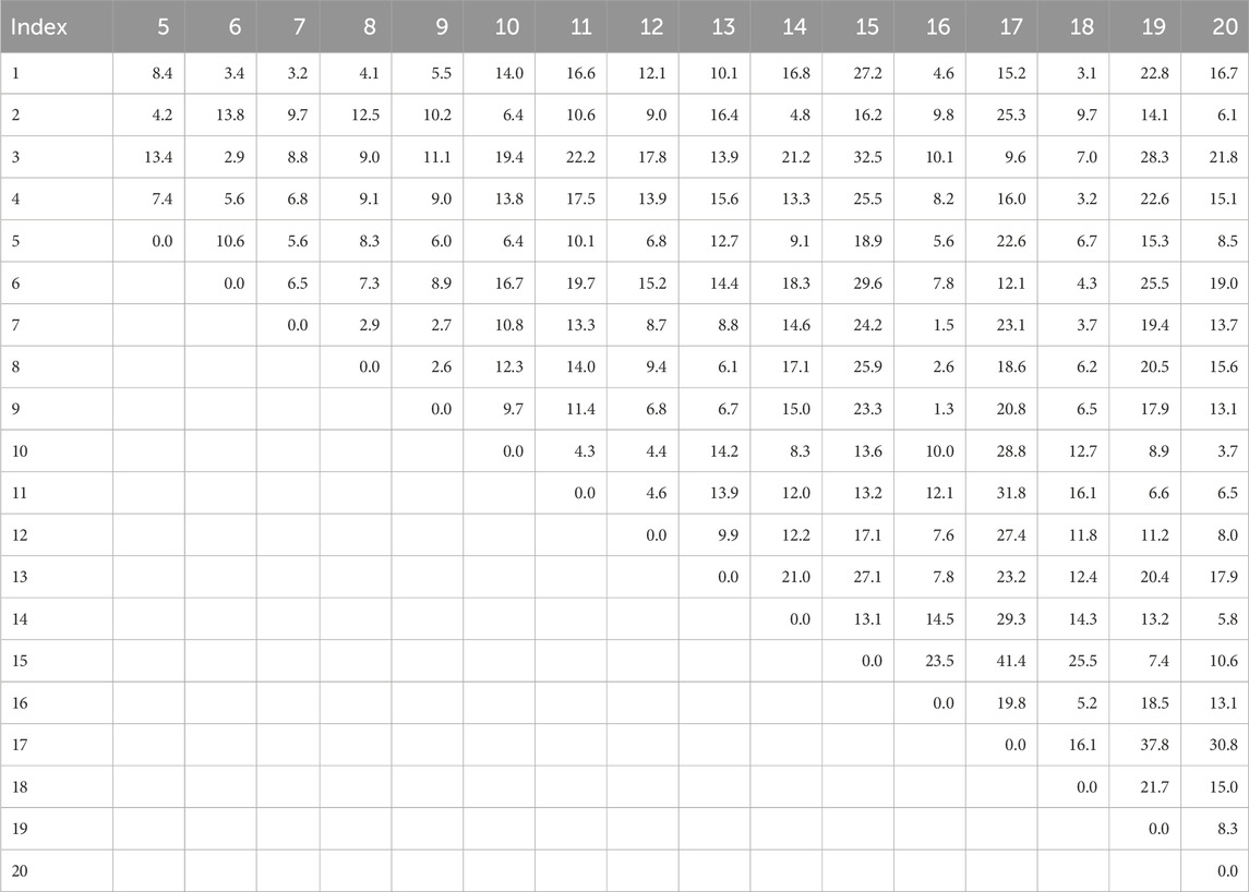
Table 13. Transportation distance in km between pairs of points.

We solve the corresponding OCLRP and CLRP with our DFWA with results in Table 14. Compared with Table 10, we observe the differences between the current distribution routes and those obtained using the OCLRP and CLRP formulations. These two not only suggest the same open depots (2 and 3) but also produce the same number of distribution vehicles (six). However, as the last row in Table 14 shows, the monthly delivery cost using OCLRP is 82965 Yuan, which is less than 93030 Yuan produced with the CLRP formulation. The savings with respect to the current distribution routes are $11.38\%$ (OCLRP) and $0.62\%$ (CLRP). These results indicate that large distribution costs can be saved if the company outsources its delivery activities to a TPL company.

Table 14

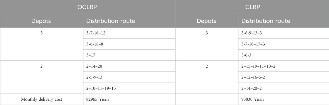
Table 14. Results obtained by implementing OCLRP and CLRP.

The same transportation and fixed vehicle costs are used for OCLRP and CLRP in the above discussion. We now analyze whether the company would still need to cooperate with a TPL provider should the unit transportation and fixed vehicle costs of the TPL company be larger than those used by the company-owned logistics. For different fixed vehicle costs, we obtained the same distribution routes shown in Table 14. Table 15 presents the monthly routing costs at different fixed vehicle costs for the OCLRP. As shown there, so long as the fixed vehicle costs are less than 2,700 Yuan, cooperation with a TPL provider seems a good option because the monthly delivery costs generated using OCLRP are less than the 93030 Yuan required if in-company logistics are used. However, when such costs are larger than 2,700 Yuan, it is better for the company to deliver the merchandise to the supermarkets through its own logistics.

Table 15

Table 15. Monthly routing costs in Yuan at different fixed vehicle costs for the OCLRP.

5 Discussion

We have studied the OCLRP, a variant of the classical CLRP, in which vehicles do not return to distribution centers or depots after having served the customers, and we proposed an effective DFWA to solve the OCLRP. This algorithm includes repeated swap moves to strengthen local search and improve solution quality. Moreover, to guarantee fireworks diversity, we implemented not only insertion and inversion moves in the mutation process but also a fitness-and-Hamming-distance-based selection strategy to select the next-generation fireworks. To verify the performance of the proposed DFWA, an extensive numerical experiment was carried out with 33 benchmark CLRP instances. Numerical results suggest that the proposed algorithm is quite competitive compared with the best-published results both in terms of solution quality and computational time. In addition, the differences between the CLRP and OCLRP solutions are further illustrated through a real case study providing improved distribution routes as well as information to support logistics outsourcing decisions.

Several potential extensions for this work include (1) developing other variants of the OCLRP, such as OCLRP with time windows, multi-objective OCLRP, and OCLRP with stochastic or fuzzy demands; (2) designing other meta-heuristic algorithms to solve the OCLRP and its variants; and (3) adapting the DFWA to solve other variants of FLPs and VRPs.

Data availability statement

Publicly available datasets were analyzed in this study. The original contributions presented in the study are included in the article/supplementary material; further inquiries can be directed to the corresponding author.

Author contributions

HZ: Supervision, Project administration, Conceptualization, Methodology, Investigation, Data curation, Writing – original draft, Writing – review and editing, Formal Analysis. XZ: Methodology, Writing – review and editing, Formal Analysis, Writing – original draft, Data curation. DR: Investigation, Writing – review and editing, Writing – original draft, Methodology.

Funding

The author(s) declare that financial support was received for the research and/or publication of this article. The research was supported by the Humanities and Social Sciences Foundation of the Ministry of Education of China (Grant No. 21YJC630087) and the High-end Foreign Experts Recruitment Plan of China (Grant No. G2023013029). The work of David Rios Insua is supported by the Spanish Ministry of Science and Research program PID2021-124662OB-I00 and the AXA-ICMAT Chair in Adversarial Risk Analysis.

Acknowledgments

The authors would like to thank all individuals and organizations who contributed directly or indirectly to this study. We also appreciate the insightful comments and suggestions provided by colleagues during the research process.

Conflict of interest

The authors declare that the research was conducted in the absence of any commercial or financial relationships that could be construed as a potential conflict of interest.

Generative AI statement

The author(s) declare that no Generative AI was used in the creation of this manuscript.

Any alternative text (alt text) provided alongside figures in this article has been generated by Frontiers with the support of artificial intelligence and reasonable efforts have been made to ensure accuracy, including review by the authors wherever possible. If you identify any issues, please contact us.

Publisher’s note

All claims expressed in this article are solely those of the authors and do not necessarily represent those of their affiliated organizations, or those of the publisher, the editors and the reviewers. Any product that may be evaluated in this article, or claim that may be made by its manufacturer, is not guaranteed or endorsed by the publisher.

References

Arifuddin, A., Utamima, A., Mahananto, F., Vinarti, R. A., and Fernanda, N. (2024). Optimizing the capacitated vehicle routing problem at pqr company: a genetic algorithm and grey wolf optimizer approach. Procedia Comput. Sci. 234, 420–427. doi:10.1016/j.procs.2024.03.023

CrossRef Full Text | Google Scholar

Bootaki, B., and Zhang, G. (2024). A location-production-routing problem for distributed manufacturing platforms: a neural genetic algorithm solution methodology. Int. J. Prod. Econ. 275, 109325. doi:10.1016/j.ijpe.2024.109325

CrossRef Full Text | Google Scholar

Chen, Y., Li, L., Zhao, X., Xiao, J., Wu, Q., and Tan, Y. (2019). Simplified hybrid fireworks algorithm. Knowledge-Based Syst. 173, 128–139. doi:10.1016/j.knosys.2019.02.029

CrossRef Full Text | Google Scholar

Dai, Z., Aqlan, F., Gao, K., and Zhou, Y. (2019). A two-phase method for multi-echelon location-routing problems in supply chains. Expert Syst. Appl. 115, 618–634. doi:10.1016/j.eswa.2018.06.050

CrossRef Full Text | Google Scholar

Ding, R., Hu, S., Xing, Z., and Yan, T. (2025). Multi-type radar deployment for uav swarms defense coverage using firework algorithm with determinantal point processes under complex terrain. Appl. Soft Comput. 170, 112681. doi:10.1016/j.asoc.2024.112681

CrossRef Full Text | Google Scholar

Erbao, C., and Mingyong, L. (2009). A hybrid differential evolution algorithm to vehicle routing problem with fuzzy demands. J. Comput. Appl. Math. 231 (1), 302–310. doi:10.1016/j.cam.2009.02.015

CrossRef Full Text | Google Scholar

Farham, M. S., Süral, H., and Iyigun, C. (2018). A column generation approach for the location-routing problem with time windows. Comput. & Operations Res. 90, 249–263. doi:10.1016/j.cor.2017.09.010

CrossRef Full Text | Google Scholar

Ferreira, K. M., and Alves de Queiroz, T. (2022). A simulated annealing based heuristic for a location-routing problem with two-dimensional loading constraints. Appl. Soft Comput. 118, 108443. doi:10.1016/j.asoc.2022.108443

CrossRef Full Text | Google Scholar

Garcia-Diaz, A., and Smith, J. M. (2024). “Facility location models,” in Facilities planning and design (Cham: Springer Nature Switzerland), 149–188.

CrossRef Full Text | Google Scholar

Garside, A. K., Ahmad, R., and Muhtazaruddin, M. N. B. (2024). A recent review of solution approaches for green vehicle routing problem and its variants. Operations Res. Perspect. 12, 100303. doi:10.1016/j.orp.2024.100303

CrossRef Full Text | Google Scholar

Kechmane, L., Nsiri, B., and Baalal, A. (2018). A hybrid particle swarm optimization algorithm for the capacitated location routing problem. Int. J. Intelligent Comput. Cybern. 11 (1), 106–120. doi:10.1108/ijicc-03-2017-0023

CrossRef Full Text | Google Scholar

Kyriakakis, N. A., Sevastopoulos, I., Marinaki, M., and Marinakis, Y. (2022). A hybrid tabu search – variable neighborhood descent algorithm for the cumulative capacitated vehicle routing problem with time windows in humanitarian applications. Comput. & Industrial Eng. 164, 107868. doi:10.1016/j.cie.2021.107868

CrossRef Full Text | Google Scholar

Marques, G., Sadykov, R., Deschamps, J.-C., and Dupas, R. (2020). An improved branch-cut-and-price algorithm for the two-echelon capacitated vehicle routing problem. Comput. & Operations Res. 114, 104833. doi:10.1016/j.cor.2019.104833

CrossRef Full Text | Google Scholar

Meng, X., and Tan, Y. (2024). Multi-guiding spark fireworks algorithm: solving multimodal functions by multiple guiding Sparks in fireworks algorithm. Swarm Evol. Comput. 85, 101458. doi:10.1016/j.swevo.2023.101458

CrossRef Full Text | Google Scholar

Mohamed, I. B., Klibi, W., Sadykov, R., Sen, H., and Vanderbeck, F. (2022). The two-echelon stochastic multi-period capacitated location-routing problem. Eur. J. Operational Res. doi:10.1016/j.ejor.2022.07.022

CrossRef Full Text | Google Scholar

Niu, Y. Y., Shao, J., Xiao, J. H., Song, W., and Cao, Z. G. (2022). Multi-objective evolutionary algorithm based on rbf network for solving the stochastic vehicle routing problem. Inf. Sci. 609, 387–410. doi:10.1016/j.ins.2022.07.087

CrossRef Full Text | Google Scholar

Nucamendi-Guillén, S., Gómez Padilla, A., Olivares-Benitez, E., and Moreno-Vega, J. M. (2021). The multi-depot open location routing problem with a heterogeneous fixed fleet. Expert Syst. Appl., 165, 113846, doi:10.1016/j.eswa.2020.113846

CrossRef Full Text | Google Scholar

Prins, C., Prodhon, C., and Calvo, R. W. (2006). Solving the capacitated location-routing problem by a grasp complemented by a learning process and a path relinking. 4(3), 221–238. doi:10.1007/s10288-006-0001-9

CrossRef Full Text | Google Scholar

Shen, X., Xu, D., Song, L., and Zhang, Y. (2023). Heterogeneous multi-project multi-task allocation in mobile crowdsensing using an ensemble fireworks algorithm. Appl. Soft Comput. 145, 110571. doi:10.1016/j.asoc.2023.110571

CrossRef Full Text | Google Scholar

Shi, Y., Zhou, Y., Boudouh, T., and Grunder, O. (2022). A memetic algorithm for a relocation-routing problem in green production of gas considering uncertainties. Swarm Evol. Comput. 74, 101129. doi:10.1016/j.swevo.2022.101129

CrossRef Full Text | Google Scholar

Tan, Y. (2015). Fireworks algorithm: a novel swarm intelligence optimization method. Incorporated: Springer Publishing Company.

Google Scholar

Tan, Y., and Zhu, Y. (2010). “Fireworks algorithm for optimization,” in Advances in swarm intelligence. ICSI 2010. Lecture notes in computer science. Editors Y. Tan, Y. Shi, and K. C. Tan (Berlin, Heidelberg: Springer), 6145, 355–364. doi:10.1007/978-3-642-13495-1_44Lect. Notes Comput. Sci.

CrossRef Full Text | Google Scholar

Tan, D., Liu, X., Zhou, R., Fu, X., and Li, Z. (2025). A novel multi-objective artificial bee colony algorithm for solving the two-echelon load-dependent location-routing problem with pick-up and delivery. Eng. Appl. Artif. Intell. 139, 109636. doi:10.1016/j.engappai.2024.109636

CrossRef Full Text | Google Scholar

Ting, C.-J., and Chen, C.-H. (2013). A multiple ant colony optimization algorithm for the capacitated location routing problem. Int. J. Prod. Econ. 141 (1), 34–44. doi:10.1016/j.ijpe.2012.06.011

CrossRef Full Text | Google Scholar

Toro, E., Franco, J. F., Echeverri, M. G., Guimarães, F. G., and Gallego Rendón, R. A. (2017). Green open location-routing problem considering economic and environmental costs. Int. J. Industrial Eng. Comput. 8 (2), 203–216. doi:10.5267/j.ijiec.2016.10.001

CrossRef Full Text | Google Scholar

Wang, Y., Sun, Y., Guan, X., Fan, J., Xu, M., and Wang, H. (2021). Two-echelon multi-period location routing problem with shared transportation resource. Knowledge-Based Syst. 226, 107168. doi:10.1016/j.knosys.2021.107168

CrossRef Full Text | Google Scholar

Yu, V. F., and Lin, S.-Y. (2015). A simulated annealing heuristic for the open location-routing problem. Comput. & Operations Res. 62, 184–196. doi:10.1016/j.cor.2014.10.009

CrossRef Full Text | Google Scholar

Yu, V. F., and Lin, S. Y. (2016). Solving the location-routing problem with simultaneous pickup and delivery by simulated annealing. Int. J. Prod. Res. 54 (2), 526–549. doi:10.1080/00207543.2015.1085655

CrossRef Full Text | Google Scholar

Zhang, H. Z., Zhang, Q., Ma, L., Zhang, Z., and Liu, Y. (2019). A hybrid ant colony optimization algorithm for a multi-objective vehicle routing problem with flexible time windows. Inf. Sci. 490, 166–190. doi:10.1016/j.ins.2019.03.070

CrossRef Full Text | Google Scholar

Zhang, H. Z., Zhang, K., Zhou, Y. Y., Ma, L., and Zhang, Z. Y. (2022a). An immune algorithm for solving the optimization problem of locating the battery swapping stations. Knowledge-Based Syst. 248, 108883–108883. doi:10.1016/j.knosys.2022.108883

CrossRef Full Text | Google Scholar

Zhang, S., Zhang, J., Zhao, Z., and Xin, C. (2022b). Robust optimization of municipal solid waste collection and transportation with uncertain waste output: a case study. J. Syst. Sci. Syst. Eng. 31, 204–225. doi:10.1007/s11518-021-5510-8

CrossRef Full Text | Google Scholar