 Esteban Acevedo-Trejos
 Gunnar Brandt
 Marco Steinacher
 Agostino Merico
- 1Systems Ecology Group, Leibniz Center for Tropical Marine Ecology, Bremen, Germany
- 2School of Engineering and Science, Jacobs University Bremen, Bremen, Germany
- 3Climate and Environmental Physics, Physics Institute, University of Bern, Bern, Switzerland
- 4Oeschger Centre for Climate Change Research, University of Bern, Bern, Switzerland
It is expected that climate change will have significant impacts on ecosystems. Most model projections agree that the ocean will experience stronger stratification and less nutrient supply from deep waters. These changes will likely affect marine phytoplankton communities and will thus impact on the higher trophic levels of the oceanic food web. The potential consequences of future climate change on marine microbial communities can be investigated and predicted only with the help of mathematical models. Here we present the application of a model that describes aggregate properties of marine phytoplankton communities and captures the effects of a changing environment on their composition and adaptive capacity. Specifically, the model describes the phytoplankton community in terms of total biomass, mean cell size, and functional diversity. The model is applied to two contrasting regions of the Atlantic Ocean (tropical and temperate) and is tested under two emission scenarios: SRES A2 or “business as usual” and SRES B1 or “local utopia.” We find that all three macroecological properties will decline during the next century in both regions, although this effect will be more pronounced in the temperate region. Being consistent with previous model predictions, our results show that a simple trait-based modeling framework represents a valuable tool for investigating how phytoplankton communities may reorganize under a changing climate.
1. Introduction
Scientists agree that Earth's climate is changing at an unprecedented rate (Pachauri and Reisinger, 2007; Wolff et al., 2014). This is expected to have an impact on all living organisms (Parmesan, 2006; Mooney et al., 2009). For example, some studies have observed a declining trend in global phytoplankton biomass during the last century (Falkowski and Wilson, 1992; Boyce et al., 2010; Mackas, 2011; Rykaczewski and Dunne, 2011), while others have proposed an increase in the abundance of marine photoautotrophs (McQuatters-Gollop et al., 2011). Irrespective of the direction of the change, it appears indisputable that any shift in the abundance of marine primary producers will have an impact on higher trophic levels (Parmesan, 2006). Scientists therefore face the challenge of better comprehending the factors and the mechanisms that will shape the marine phytoplankton community in the decades to come.
Natural ecological communities are typically studied by gathering information about, for example, physiological and morphological properties on a predefined taxon. This generally treats all species as identical and neglects property variations within the taxon (Violle et al., 2012). An alternative approach is to gather information on the distribution of such properties within the entire community (McGill et al., 2006). This is the so-called trait-based approach (McGill et al., 2006), which provides a conceptual framework for understanding how communities are organized and adapted to given environmental conditions and how they will reorganize under a changing climate. Fundamental constraints, such as energy allocation, prevent organisms to invest equally in all traits and lead to the emergence of trade-offs, which in turn give rise to functionally diverse communities (Tilman, 2001).
By identifying key traits and trade-offs, the trait-based approach has advanced our understanding of phytoplankton community structure and functioning (Litchman et al., 2007; Litchman and Klausmeier, 2008) and provided the basis for constructing mechanistic links between community composition and environmental conditions (Follows and Dutkiewicz, 2011; Smith et al., 2011). In addition, the distribution of traits reflects the functional diversity of the community and hence its adaptive capacity (Abrams et al., 1993). Cell size, for example, has been proposed as the most characterizing morphological trait of phytoplankton organisms (Litchman and Klausmeier, 2008; Finkel et al., 2009). It spans over several orders of magnitude only within phytoplankton and influences many ecological and physiological processes, such as nutrient uptake (Aksnes and Egge, 1991; Tang, 1995; Litchman et al., 2007; Marañón et al., 2013), light harvesting (Ciotti et al., 2002; Finkel et al., 2004), respiration (Laws, 1975; López-Urrutia et al., 2006), sinking (Kiørboe, 1993), and grazing (Kiørboe, 1993; Fuchs and Franks, 2010; Wirtz, 2012a,b). Therefore, investigating the dynamics of phytoplankton cell size helps to better understand the adaptive capacity of this group of organisms under a changing environment.
Size-based models of phytoplankton communities in combination with climate projections provide a useful tool for these investigations. Models following the species-by-species approach (e.g., Baird and Suthers, 2007; Banas, 2011) typically comprise many state variables and parameters. While valuable, such models have been criticized for the high number of free parameters required to adequately describe the observed macroecological properties of planktonic communities (Anderson, 2005; Ward et al., 2010). Alternatively, many scientists (e.g., Litchman and Klausmeier, 2008; Follows and Dutkiewicz, 2011; Smith et al., 2011; Edwards et al., 2013) have called for the use of trait-based modeling approaches to investigate how phytoplankton community structure and diversity may reorganize under a changing climate. No study to date has yet attempted to investigate the effects of future climate on the combined dynamics of phytoplankton biomass and trait distributions.
Here we use a novel size-based model of aggregate group properties that mechanistically describes phytoplankton community structure and functional diversity in two contrasting regions of the Atlantic Ocean (i.e., temperate and tropical). The model focuses on three macroecological properties, namely: total phytoplankton biomass, mean cell size, and size variance, the latter reflecting the functional diversity of the community and therefore its adaptive capacity. We run the model into the future using two distinct projections of the IPCC emission scenarios (Nakićenović et al., 2000), which are routinely used for studying the transitions of ecosystems. These are: the “a divided world” (SRES A2) scenario (also known as “business as usual”), which assumes emphasis on national identities, and the more optimistic “local utopia” (SRES B1) scenario, which assumes a moderate reduction in material demand and a moderate use of clean and efficient technologies but still with a pronounced regionalization of the economies. With this model we investigate how the structure and adaptive capacity of phytoplankton communities will respond to changing environmental conditions.
2. Methods
2.1. Size-Based Model
We developed a size-based model of the upper mixed-layer to study the future composition of phytoplankton communities under different climate change scenarios. The model focuses on the description of three macroecological properties: total phytoplankton biomass (P), phytoplankton cell size (S, expressed as Equivalent Spherical Diameter (ESD)), and size variance (V). In this type of models the trait variance reflects the functional diversity of the community (Wirtz and Eckhardt, 1996; Norberg et al., 2001; Merico et al., 2009) and quantifies the speed of the adaptive process, i.e., the speed with which the mean trait changes (Abrams et al., 1993). Given that adaptive responses are considered to be more robust for more diverse communities (Visser, 2008), the size variance captured by our model is also a representation of the adaptive capacity of the phytoplankton community. This means that the higher the trait variance, the higher the functional diversity and the adaptive capacity of the system, and vice versa. Instead of resolving the full spectrum of species or functional types, this modeling approach centers on aggregate properties of the entire planktonic community thus reducing model complexity (Merico et al., 2009) and mechanistically linking community structure with environmental conditions (Wirtz and Eckhardt, 1996; Norberg et al., 2001). In the model, the phytoplankton communities self-assemble based on a trade-off emerging from relationships between phytoplankton mean size and: (1) phytoplankton nutrient uptake, (2) zooplankton grazing, and (3) phytoplankton sinking. Equations for nutrient (N), zooplankton (Z), and detritus (D) complete the model system (see Appendix for a detailed description of all model equations).
2.2. Studied Regions
The model is applied to two contrasting regions of the Atlantic Ocean: temperate (45.5–49.5 °N, 10.5–20.5 °W) and tropical (4.5–14.5 °N, 19.5–24.5 °W). The temperate region is characterized by seasonal changes of mixed layer depth (MLD), sea surface temperature (SST), photosynthetic active radiation (PAR), and concentration of nutrients below the mixed layer (N0), whereas environmental conditions in the tropical region are relatively constant. Note that the model parameterization is identical for the two regions and that different results emerge only from the contrasting environmental forcing (see Table 1). Hereafter, we will use the terminology “environmental variables,” to refer to all variables that force the model (i.e., MLD, SST, PAR, N0).
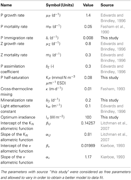
Table 1. Model parameters (identical for both regions).
2.3. Environmental Forcing Data
The environmental variables used to force the ecosystem model are derived from simulations with the NCAR CSM1.4-carbon model (Fung et al., 2005; Doney et al., 2006). The NCAR model is one of the global Earth system models that are used to study past and future impacts of anthropogenic emissions on the environment (e.g., Steinacher et al., 2010) and contributed to previous assessment reports of the IPCC. The NCAR model was driven by historical CO2 emissions over the industrial period, followed by two IPCC scenarios for the 21st century: SRES A2, a “business-as-usual” scenario in which atmospheric CO2 reaches 840 ppm by 2100 AD, and SRES B1, a convergent world scenario in which CO2 concentrations stabilize at about 540 ppm by 2100 AD (Nakićenović et al., 2000). A more detailed description of the simulations is given by Steinacher et al. (2009).
From the comprehensive NCAR model output, we use MLD, SST, PAR, and N0, which are available at a monthly resolution on a grid with a resolution of 3.6° in longitude and 0.8–1.8° in latitude. The gridded variables are then spatially averaged within each region to obtain time series over the period of the simulation for both scenarios. PAR (in W · m−2) is calculated from the solar heat flux at the ocean surface (in K · cm · s−1) by applying a conversion factor of 4.1 · 104 J · m−2 · cm−1 · K−1. Since the biogeochemistry module of the NCAR model is defined in units of phosphorus, we consider the Redfield N:P ratio of 16:1 whenever a conversion to units of nitrogen is needed.
2.4. Analysis of Annual Trends of P, S, and V
We apply a Principal Component Analysis, PCA (Mantua, 2004) to conduct an exploratory statistical analysis with annually averaged variables of the size-based model and the environmental forcing. With the PCA we identify the general patterns of variability from a number of time series by means of reducing the dimensionality of the dataset into a small number of uncorrelated principal components (von Storch and Zwiers, 2001). Typically, the first principal component has the highest eigenvalue and, as new orthogonal components are added, the eigenvalues of new components decrease. These eigenvalues are interpreted as the amount of variability explained by each principal component (Supplementary Figure 1). Another important output of the PCA is represented by the eigenvectors or loadings, which reflect the relative importance of each variable on each principal component. PCA has been widely used to explore multivariate time series in particular with respect to the detection of regime shifts (e.g., Hare and Mantua, 2000; Mantua, 2004; Weijerman et al., 2005; Schlüter et al., 2012).
In addition, we use probabilistic models based on the generalized least squares method to analyse the long-term trends of the state variables that describe structure and diversity of the two phytoplankton communities (i.e., total biomass, mean trait, and trait variance). We adopted this statistical approach, because it allows us to correct the data for temporal correlations and for unequal variances (Zuur et al., 2009). Each fit is evaluated by a visual inspection of the residuals. To better understand the long-term trends of phytoplankton community structure and diversity under the two emission scenarios we subdivide the time series into three main periods: (1) past, which corresponds to the period from 1850 to 2000 and is the same for both scenarios, (2) future-A2, which corresponds to the period from 2000 to 2100 of the business as usual scenario, and (3) future-B1, which corresponds to the period from 2000 to 2100 of the convergent world scenario. First, the probabilistic models are fitted to each of the three periods and two regions using the variables P, S, and V as response variables and using time as the explanatory variable. Second, we perform an analysis of variance (ANOVA) with the slopes of each probabilistic model as response variables, and periods (past, future-A2, and future-B1) and regions (temperate and tropical) as explanatory variables.
3. Results
Figure 1 summarizes all the environmental variables used to force our size-based model. The emission scenarios are identical in the period from 1850 to 2000, but differ from 2000 to 2100. The strongest difference between the two scenarios is in SST, whereas the other three environmental variables show similar variability (Figure 1).
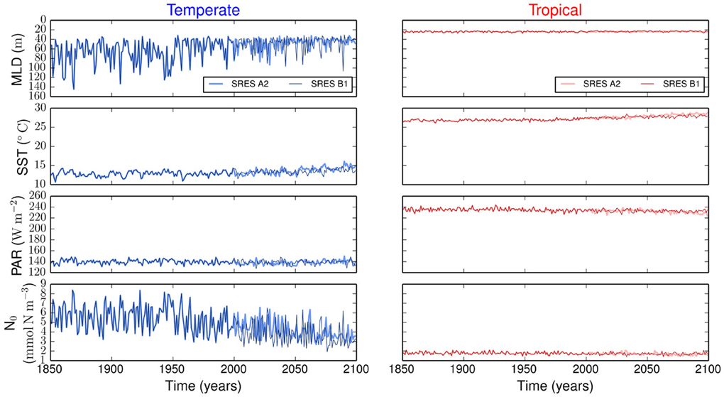
Figure 1. Environmental forcing for temperate and tropical regions under the SRES A2 and the SRES B1 emission scenarios. MLD is the mixed layer depth, PAR is the photosynthetically active radiation, SST is the sea surface temperature, and N0 is the concentration of nutrients below the upper mixed-layer.
The resulting simulations reveal no major differences in phytoplankton community composition between emission scenarios (Supplementary Figure 1). Strong differences are observed between regions. Our results show that the variability is stronger in the temperate region than in the tropical region (Figure 2). In the temperate region, the projected increase in SST leads to a more stratified ocean, which is expressed by the shoaling of the MLD (Figure 1). The amplitude of the fluctuations in nutrient concentration reduces after the year 2000. This long-term decline in nutrient concentration reflects the change exhibited by the MLD and drives the decreases in P, S, and V. The changes in total phytoplankton biomass appear to cause a baseline shift toward smaller concentrations of Z and D. In contrast, the tropical region shows weaker or no trends in all state variables (Figure 2).
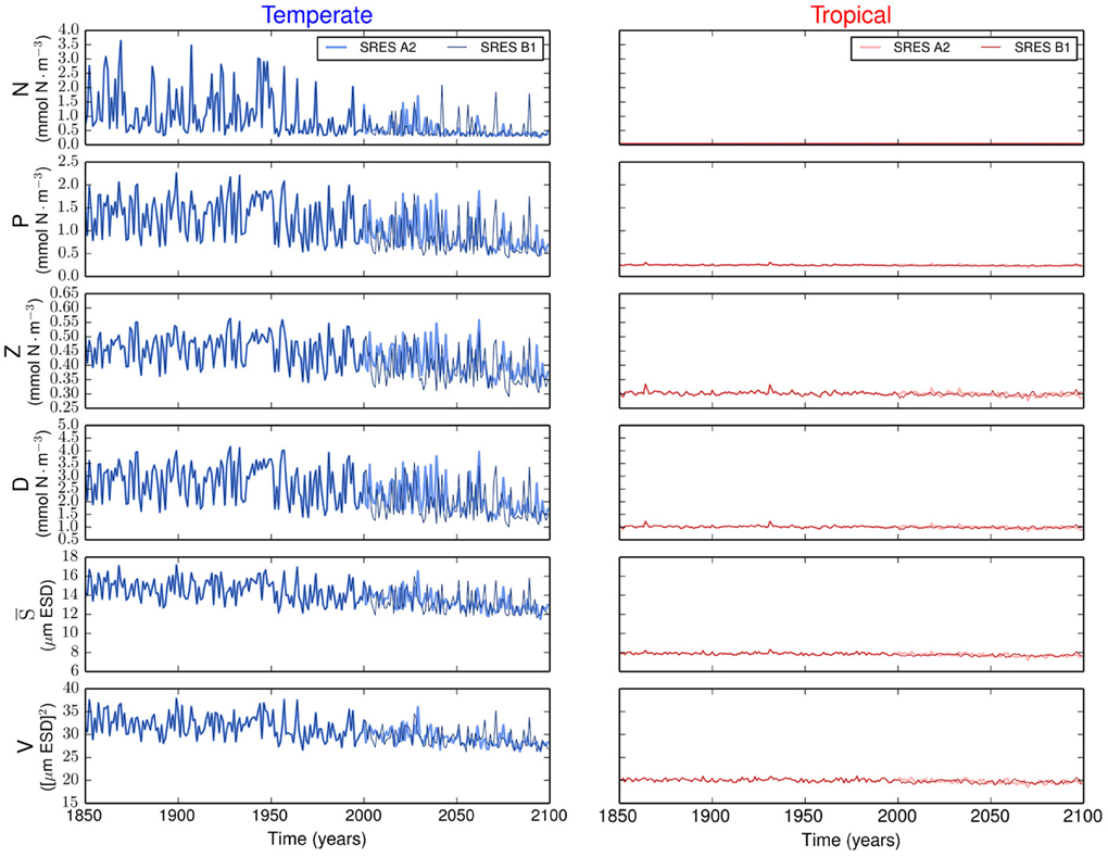
Figure 2. Time series of the state variables for the temperate and tropical regions under the SRES A2 and the SRES B1 emission scenarios. N is the nutrient concentration, P is the phytoplankton concentration, Z is the zooplankton concentration, D is the detritus concentration, S is the phytoplankton mean size, and V is the size variance or functional diversity of phytoplankton.
The first principal component explains over 55 % of the variation in the datasets (Supplementary Figure 1). The scores on the first principal component of the PCA reveal the existence of two regimes, which are linked by a rather smooth transition (Figure 3). While the first regime from 1850 to approximately 2000 is dominated by negative scores on the first principal component, the second regime from 2000 to 2100 is characterized by mostly positive scores on the first principal component (Figure 3). This analysis also reveals that the environmental drivers of the major mode of variability represented by the first principal component are temperature (SST) and nutrient availability, the latter determined by MLD and N0 (Figure 4). These variables, in fact, have the highest positive and negative loadings on the first principal component for both, the two scenarios and the two regions (Figure 4).
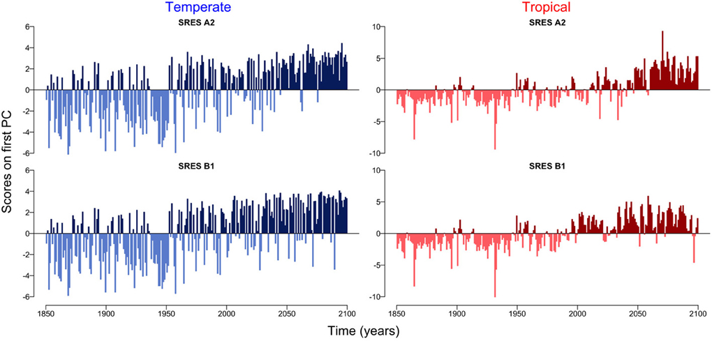
Figure 3. Scores on the first principal component for temperate and tropical regions under the SRES A2 and SRES B1 emission scenarios.
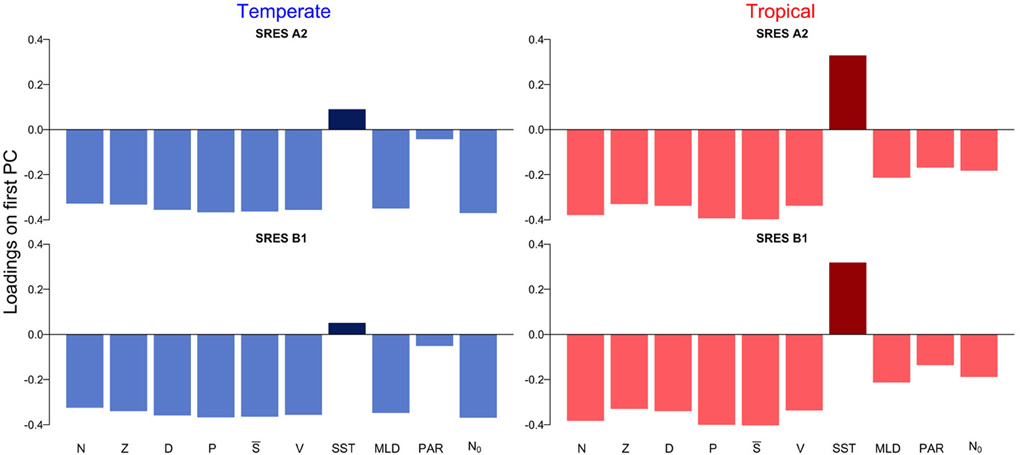
Figure 4. Loadings on the first principal component for temperate and tropical regions under the SRES A2 and SRES B1 emission scenarios.
All three periods (i.e., past, future-A2, and future-B1), show declining trends in both regions (Figure 5). However, there are no differences in the slopes of the trends (Supplementary Figure 2), between periods (ANOVA, df: 2, F-value: 1.9542, p-value: 0.1842) or between regions by periods (ANOVA, df: 2, F-value: 0.2749, p-value: 0.7643). The only significant difference in the slopes is between regions (ANOVA, df: 1, F-value: 10.9999, p-value: 0.0061). The declining trends are steepest in the future-A2 period (Supplementary Figure 2). More specifically, the temperate Atlantic appears to be more sensitive since it will experience the largest decline among all scenarios in phytoplankton mean size (S) and functional diversity (V), with approximately −1.8 (μm ESD century−1) and −3.1 ([μm ESD]2 century−1) (Supplementary Figure 2). Our results also suggest that the tropical region will be less affected than the temperate region with less than 0.3 decline in P (mmol N m−3century−1), S (μm ESD century−1), and V ([μm ESD]2 century−1) (Supplementary Figure 2).
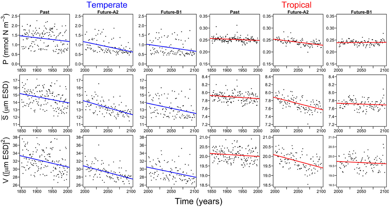
Figure 5. Probabilistic model fits of the annual trends of the phytoplankton state variables for temperate and tropical regions and for the three different time periods (i.e., past, future-A2, and future-B1). P is the phytoplankton concentration, S is the phytoplankton mean size, and V is the size variance or functional diversity of phytoplankton. The color lines represent the generalized least square fits for temperate and tropical regions.
In addition, we performed a sensitivity analysis in which we varied all the model parameters by ± 25% and quantified the effect of such change on the annual trends of the three periods (Figures 6–8). The greatest effects arise in the parameters that control phytoplankton grazing, i.e., μZ. A decrease in μZ by 25% produces up to an 1.5-fold decrease in the declining trend of P and also an increase in the slopes of S and V of, respectively, 6-fold and 3-fold (Figures 6–8). As expected, increasing μZ by 25% causes opposite effects on the slopes of P, S, and V, however, with a lower magnitude compared to the equivalent decrease of μZ (Figures 6–8). Another sensitive parameter is the density-dependent immigration rate (δI), which mainly affects V and S for the tropical region under scenario B1 (Figures 6–8). Changes in the light attenuation coefficient kw showed an impact only in the temperate region under past conditions (Figure 6). This probably reflects an overestimation of the effects of light attenuation in the temperate region (see Appendix) due to the weaker stratification in the past as compared to the future scenarios.
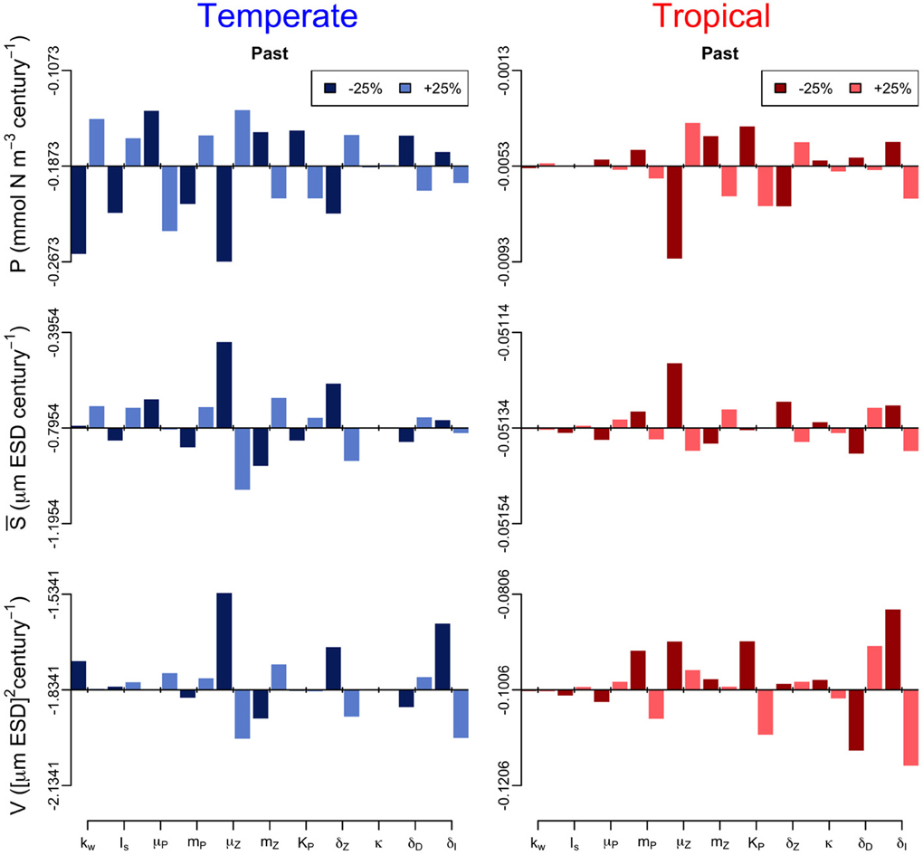
Figure 6. Sensitivity analysis of the phytoplankton state variables (P, S, and V) to ± 25% changes in the values of the model parameters for the past period. The origin of each panel corresponds to the magnitude of the slope quantified in Supplementary Figure 2, and the bars represent the effect of the 25% alterations. For further details on the parameter values used see Table 1.
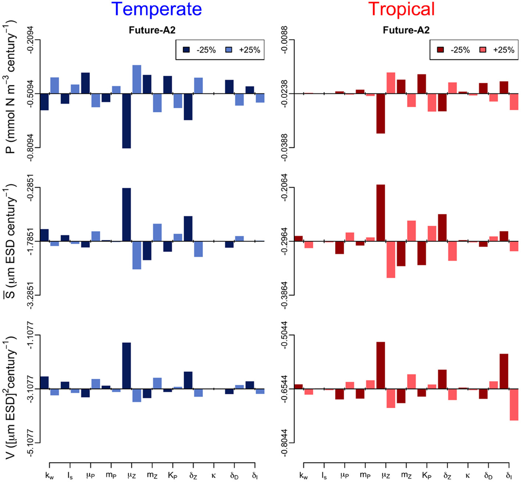
Figure 7. Sensitivity analysis of the phytoplankton state variables (P, S, and V) to ± 25% changes in values of the model parameters for the future-A2 period. The origin of each panel corresponds to the magnitude of the slope quantified in Supplementary Figure 2, and the bars represent the effect of the 25% alterations. For further details of the parameters used see Table 1.
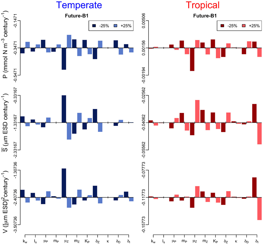
Figure 8. Sensitivity analysis of the phytoplankton state variables (P, S, and V) to ± 25% changes in the values of the model parameters for the future-B1 period. The origin of each panel corresponds to the magnitude of the slope quantified in Supplementary Figure 2, and the bars represent the effect of the 25% alterations. For further details of the parameters used see Table 1.
4. Discussion
We used a size-based model to explore the composition of two different phytoplankton communities (tropical and temperate) under past environmental conditions and future climate change scenarios. The model was previously calibrated and tested against present day observations of nutrient concentrations and phytoplankton biomass (see Supplementary Figure 3).
Most projections of the future climate suggest that the world oceans will become warmer and more stratified than present (Pachauri and Reisinger, 2007; Steinacher et al., 2010; Reusch and Boyd, 2013; Wolff et al., 2014). Such warming will likely lead to a shallower upper mixed-layer and thus to a reduced nutrient supply from the deep ocean (Steinacher et al., 2010; Reusch and Boyd, 2013). Our model experiments generally confirm this view, but further show that the expected changes will differ considerably by ocean region. In contrast, the different future scenarios produce minor changes in the model results (Figure 1). In our simulations, the temperate region will experience strongest changes in MLD, SST, and N0 by the year 2100 (Figure 1). These changes will lead to a decline in average phytoplankton biomass, mean cell size, and functional diversity (i.e., adaptive capacity), see Figure 2. The tropical region will experience comparatively less environmental changes than the temperate region (Figure 1) and, consequently, less alterations in phytoplankton community composition (Figure 2). Contrasting differences in phytoplankton community structure between tropical and temperate regions are well known biogeographical features of the modern ocean (Marañón et al., 2001) and our results suggest that these differences will be maintained also in the future. Analogously to the results presented here, a previous multi-species and multi-nutrient modeling study showed that a surface ocean with less mixing and hence less nutrients will favor smaller phytoplankton species (Litchman et al., 2006).
Accumulating evidence suggests that a changing climate has and will have dramatic consequences on the Earth's biota (Parmesan, 2006). In planktonic ecosystems, for example, changes in the environment have entailed shifts in the phenology of phytoplankton (Schlüter et al., 2012) and zooplankton (Schlüter et al., 2010) causing mismatches between trophic levels and functional groups (Edwards and Richardson, 2004). The quantitative analysis of the temporal patterns of the two planktonic ecosystems in the Atlantic Ocean show two apparently distinct regimes, the first from 1850 to 2000 and the second from 2000 to 2100 (Figure 3). The two regimes are, however, not separated by an abrupt shift as observed, for example, in the Pacific Ocean (Hare and Mantua, 2000), in the North Sea (Beaugrand, 2004; Weijerman et al., 2005) and in the German Bight (Schlüter et al., 2008), but are rather linked by a very smooth transition (Figure 3). Note that the low signal to noise ratio typical of phytoplankton time-series may hinder the detection of patterns or key drivers of change (Winder and Cloern, 2010). To minimize the effect of potential noise on our results and to avoid the over-interpretation of short-term fluctuations, we focused our analyses on long-term trends (i.e., decades to centuries) of temporally and spatially averaged variables.
The quantitative analyses of the long-term trends in the three macroecological properties show a decline in P, S, and V (Figure 5), with the major differences arising between regions. The temperate Atlantic will be the region to experience the highest rates of decline (Supplementary Figure 2), in terms of phytoplankton cell sizes and functional diversity. It has been suggested that a changing climate, specifically an increase in SST, will lead to a dominance of small phytoplankton cells in the oceans (Daufresne, 2009; Morán et al., 2010). However, other studies have questioned this conclusion providing empirical evidence for a stronger effect of nutrients rather than of SST on the size structure of phytoplankton communities (Marañón et al., 2012). Our simulations suggest a combined effect of SST and nutrient availability, with the latter being governed by changes in MLD and N0 (Figure 4). This finding is also consistent with a recent empirical biogeographical classification of the phytoplankton size distribution in the global ocean (Acevedo-Trejos et al., 2013) suggesting that the most parsimonious model of size structure can be defined by nutrient availability and temperature. Nevertheless, none of the mentioned theoretical and empirical studies has linked in a single framework, as we do here, the size composition and the adaptive capacity of the community to future changes of the environment.
Our modeling approach focuses on phytoplankton community structure and functional diversity and treats zooplankton as an assemblage of many identical individuals. We thus disregard the variety of different feeding mechanisms in zooplankton and their potential impact on the phytoplankton community (see Gentleman et al., 2003, for a review on functional responses of zooplankton). However, to assess the sensitivity of our results to this model simplification, we performed an in-depth sensitivity analysis on the role of zooplankton grazing in structuring the two phytoplankton communities (Figures 6–8). Specifically, we found that an increase in grazing pressure would exacerbate the declining trends in S, and V. Analogously, a decrease in grazing pressure would attenuate the declining trends in the two variables. While this finding highlights the fundamental role of grazing in defining phytoplankton size distributions, a more detailed description of zooplankton, e.g., including different zooplankton size classes, life stages, feeding preferences, etc. (e.g., Banas, 2011; Prowe et al., 2012; Wirtz, 2012a; Mariani et al., 2013), would probably improve the quality of our projections (Wirtz, 2012a; Smith et al., 2014). However, an adequate description of the adaptive responses of grazers is still a topic of ongoing research (Litchman et al., 2013; Smith et al., 2014) and a consistent and well accepted formulation that takes into account all relevant zooplankton-phytoplankton interaction processes is still lacking.
In summary, our study suggests that under a warmer and more stratified ocean phytoplankton communities will shift toward smaller mean size and will lose adaptive capacity in the process. These changes will be more pronounced in regions with strong seasonal variations and will be additionally modulated by potential modifications in grazing pressure.
Author Contributions
Agostino Merico and Gunnar Brandt conceived the idea of the study; Esteban Acevedo-Trejos coded the model and performed the analyses; Marco Steinacher provided the environmental forcing data from GCM simulations; all authors contributed to interpret the results and to write the manuscript.
Conflict of Interest Statement
The authors declare that the research was conducted in the absence of any commercial or financial relationships that could be construed as a potential conflict of interest.
Supplementary Material
The Supplementary Material for this article can be found online at: http://www.frontiersin.org/journal/10.3389/fmars.2014.00015/abstract
References
Abrams, P., Matsuda, H., and Harada, Y. (1993). Evolutionarily unstable fitness maxima and stable fitness minima of continuous traits. Evol. Ecol. 7, 465–487. doi: 10.1007/BF01237642
Acevedo-Trejos, E., Brandt, G., Merico, A., and Smith, S. L. (2013). Biogeographical patterns of phytoplankton community size structure in the oceans. Glob. Ecol. Biogeogr. 22, 1060–1070. doi: 10.1111/geb.12071
Aksnes, D. L., and Egge, J. K. (1991). A theoretical model for nutrient uptake in phytoplankton. Mar. Ecol. Prog. Ser. 70, 65–72. doi: 10.3354/meps070065
Anderson, T. R. (2005). Plankton functional type modelling: running before we can walk? J. Plankton Res. 27, 1073–1081. doi: 10.1093/plankt/fbi076
Baird, M. E., and Suthers, I. M. (2007). A size-resolved pelagic ecosystem model. Ecol. Modelling 203, 185–203. doi: 10.1016/j.ecolmodel.2006.11.025
Banas, N. S. (2011). Adding complex trophic interactions to a size-spectral plankton model: emergent diversity patterns and limits on predictability. Ecol. Modelling 222, 2663–2675. doi: 10.1016/j.ecolmodel.2011.05.018
Beaugrand, G. (2004). The North Sea regime shift: evidence, causes, mechanisms and consequences. Prog. Oceanogr. 60, 245–262. doi: 10.1016/j.pocean.2004.02.018
Boyce, D. G., Lewis, M. R., and Worm, B. (2010). Global phytoplankton decline over the past century. Nature 466, 591–596. doi: 10.1038/nature09268
Ciotti, A. M., Lewis, M. R., and Cullen, J. J. (2002). Assessment of the relationships between dominant cell size in natural phytoplankton communities and the spectral shape of the absorption coefficient. Limnol. Oceanogr. 47, 404–417. doi: 10.4319/lo.2002.47.2.0404
Daufresne, M. (2009). Global warming benefits the small in aquatic ecosystems. Proc. Natl. Acad. Sci. U.S.A. 106, 12788–12793. doi: 10.1073/pnas.0902080106
Doney, S., Lindsay, K., Fung, I., and John, J. (2006). Natural variability in a stable, 1000-yr global coupled climateŞcarbon cycle. J. Clim. 19, 3033–3054. doi: 10.1175/JCLI3783.1
Edwards, A., and Brindley, J. (1996). Oscillatory behaviour in a three-component plankton population model. Dyn. Stabil. Syst. 11, 347–370. doi: 10.1080/02681119608806231
Edwards, K. F., Litchman, E., and Klausmeier, C. A. (2013). Functional traits explain phytoplankton community structure and seasonal dynamics in a marine ecosystem. Ecol. Lett. 16, 56–63. doi: 10.1111/ele.12012
Edwards, M., and Richardson, A. J. (2004). Impact of climate change on marine pelagic phenology and trophic mismatch. Nature 430, 881–884. doi: 10.1038/nature02808
Falkowski, P. G., and Wilson, C. (1992). Phytoplankton productivity in the North Pacific ocean since 1900 and implications for absorption of anthropogenic CO2. Nature 358, 741–743. doi: 10.1038/358741a0
Fasham, M. (1993). “Modelling the marine biota,” in The Global Carbon Cycle, ed M. Heimann (Heidelberg: Springer-Verlag), 457–504.
Fasham, M., Ducklow, H., and Mckelvie, S. M. (1990). A nitrogen-based model of plankton dynamics in the oceanic mixed layer. J. Mar. Res. 48, 591–639. doi: 10.1357/002224090784984678
Finkel, Z. V., Beardall, J., Flynn, K. J., Quigg, A., Rees, T. A. V., and Raven, J. A. (2009). Phytoplankton in a changing world: cell size and elemental stoichiometry. J. Plankton Res. 32, 119–137. doi: 10.1093/plankt/fbp098
Finkel, Z. V., Irwin, A. J., and Schofield, O. (2004). Resource limitation alters the 3/4 size scaling of metabolic rates in phytoplankton. Mar. Ecol. Prog. Ser. 273, 269–279. doi: 10.3354/meps273269
Follows, M. J., and Dutkiewicz, S. (2011). Modeling diverse communities of marine microbes. Ann. Rev. Mar. Sci. 3, 427–451. doi: 10.1146/annurev-marine-120709-142848
Fuchs, H. L., and Franks, P. J. (2010). Plankton community properties determined by nutrients and size-selective feeding. Mar. Ecol. Prog. Ser. 413, 1–15. doi: 10.3354/meps08716
Fung, I. Y., Doney, S. C., Lindsay, K., and John, J. (2005). Evolution of carbon sinks in a changing climate. Proc. Natl. Acad. Sci. U.S.A. 102, 11201–11206. doi: 10.1073/pnas.0504949102
Gentleman, W., Leising, A., Frost, B., Strom, S., and Murray, J. (2003). Functional responses for zooplankton feeding on multiple resources: a review of assumptions and biological dynamics. Deep Sea Res. II Top. Stud. Oceanogr. 50, 2847–2875. doi: 10.1016/j.dsr2.2003.07.001
Hare, S., and Mantua, N. (2000). Empirical evidence for North Pacific regime shifts in 1977 and 1989. Prog. Oceanogr. 47, 103–145. doi: 10.1016/S0079-6611(00)00033-1
Kiørboe, T. (1993). Turbulence, phytoplankton cell size, and the structure of pelagic food webs. Adv. Mar. Biol. 29, 1–72. doi: 10.1016/S0065-2881(08)60129-7
Laws, E. (1975). The importance of respiration losses in controlling the size distribution of marine phytoplankton. Ecology 56, 419–426. doi: 10.2307/1934972
Litchman, E., and Klausmeier, C. A. (2008). Trait-based community ecology of phytoplankton. Ann. Rev. Ecol. Evol. Syst. 39, 615–639. doi: 10.1146/annurev.ecolsys.39.110707.173549
Litchman, E., Klausmeier, C. A., Miller, J. R., Schofield, O., and Falkowski, P. G. (2006). Multi-nutrient, multi-group model of present and future oceanic phytoplankton communities. Biogeosciences 3, 585–606. doi: 10.5194/bg-3-585-2006
Litchman, E., Klausmeier, C. A., Schofield, O., and Falkowski, P. G. (2007). The role of functional traits and trade-offs in structuring phytoplankton communities: scaling from cellular to ecosystem level. Ecol. Lett. 10, 1170–1181. doi: 10.1111/j.1461-0248.2007.01117.x
Litchman, E., Ohman, M. D., and Kiorboe, T. (2013). Trait-based approaches to zooplankton communities. J. Plankton Res. 35, 473–484. doi: 10.1093/plankt/fbt019
López-Urrutia, A., San Martin, E., Harris, R. P., and Irigoien, X. (2006). Scaling the metabolic balance of the oceans. Proc. Natl. Acad. Sci. U.S.A. 103, 8739–8744. doi: 10.1073/pnas.0601137103
Mackas, D. L. (2011). Does blending of chlorophyll data bias temporal trend? Nature 472, E4–E5. doi: 10.1038/nature09951
Mantua, N. (2004). Methods for detecting regime shifts in large marine ecosystems: a review with approaches applied to North Pacific data. Prog. Oceanogr. 60, 165–182. doi: 10.1016/j.pocean.2004.02.016
Marañón, E., Cermeño, P., Latasa, M., and Tadonléké, R. D. (2012). Temperature, resources, and phytoplankton size structure in the ocean. Limnol. Oceanogr. 57, 1266–1278. doi: 10.4319/lo.2012.57.5.1266
Marañón, E., Cermeño, P., López-Sandoval, D. C., Rodríguez-Ramos, T., Sobrino, C., Huete-Ortega, M., et al. (2013). Unimodal size scaling of phytoplankton growth and the size dependence of nutrient uptake and use. Ecol. Lett. 16, 371–379. doi: 10.1111/ele.12052
Marañón, E., Holligan, P., Barciela, R., González, N., Mouriño, B., Pazó, M., et al. (2001). Patterns of phytoplankton size structure and productivity in contrasting open-ocean environments. Mar. Ecol. Prog. Ser. 216, 43–56. doi: 10.3354/meps216043
Mariani, P., Andersen, K. H., Visser, A. W., Barton, A. D., and Kiørboe, T. (2013). Control of plankton seasonal succession by adaptive grazing. Limnol. Oceanogr. 58, 173–184. doi: 10.4319/lo.2013.58.1.0173
McGill, B. J., Enquist, B. J., Weiher, E., and Westoby, M. (2006). Rebuilding community ecology from functional traits. Trends Ecol. Evol. 21, 178–185. doi: 10.1016/j.tree.2006.02.002
McQuatters-Gollop, A., Reid, P., Edwards, M., Burkill, P., Castellani, C., Batten, S., et al. (2011). Is there a decline in marine phytoplankton? Nature 472, E6–E7. doi: 10.1038/nature09950
Merico, A., Bruggeman, J., and Wirtz, K. (2009). A trait-based approach for downscaling complexity in plankton ecosystem models. Ecol. Modelling 220, 3001–3010. doi: 10.1016/j.ecolmodel.2009.05.005
Merico, A., Tyrrell, T., Lessard, E. J., Oguz, T., Stabeno, P. J., Zeeman, S. I., et al. (2004). Modelling phytoplankton succession on the Bering Sea shelf: role of climate influences and trophic interactions in generating Emiliania huxleyi blooms 19972000. Deep Sea Res. I 51, 1803–1826. doi: 10.1016/j.dsr.2004.07.003
Mooney, H., Larigauderie, A., Cesario, M., Elmquist, T., Hoegh-Guldberg, O., Lavorel, S., et al. (2009). Biodiversity, climate change, and ecosystem services. Curr. Opin. Environ. Sustain. 1, 46–54. doi: 10.1016/j.cosust.2009.07.006
Morán, X. A. G., López-Urrutia, A., Calvo-Díaz, A., and Li, W. K. W. (2010). Increasing importance of small phytoplankton in a warmer ocean. Glob. Change Biol. 16, 1137–1144. doi: 10.1111/j.1365-2486.2009.01960.x
Nakićenović, N., Alcamo, J., Davis, G., Grübler, A., Kram, T., Lebre La Rovere, E., et al. (2000). Special Report on Emissions Scenarios. New York, NY: Intergovernmental Panel on Climate Change, Cambridge University Press.
Norberg, J., Swaney, D. P., Dushoff, J., Lin, J., Casagrandi, R., and Levin, S. A. (2001). Phenotypic diversity and ecosystem functioning in changing environments: a theoretical framework. Proc. Natl. Acad. Sci. U.S.A. 98, 11376–11381. doi: 10.1073/pnas.171315998
Pachauri, R. K., and Reisinger, A. (eds.). (2007). Climate Change 2007: Synthesis Report. Geneva: IPPC.
Parmesan, C. (2006). Ecological and evolutionary responses to recent climate change. Ann. Rev. Ecol. Evol. Syst. 37, 637–669. doi: 10.1146/annurev.ecolsys.37.091305.110100
Prowe, A. F., Pahlow, M., Dutkiewicz, S., Follows, M. J., and Oschlies, A. (2012). Top-down control of marine phytoplankton diversity in a global ecosystem model. Prog. Oceanogr. 101, 1–13. doi: 10.1016/j.pocean.2011.11.016
Reusch, T. B. H., and Boyd, P. W. (2013). Experimental evolution meets marine phytoplankton. Evolution 67, 1849–1859. doi: 10.1111/evo.12035
Rykaczewski, R. R., and Dunne, J. P. (2011). A measured look at ocean chlorophyll trends. Nature 472, E5–E6. doi: 10.1038/nature09952
Schlüter, M. H., Kraberg, A., and Wiltshire, K. H. (2012). Long-term changes in the seasonality of selected diatoms related to grazers and environmental conditions. J. Sea Res. 67, 91–97. doi: 10.1016/j.seares.2011.11.001
Schlüter, M. H., Merico, A., Reginatto, M., Boersma, M., Wiltshire, K. H., and Greve, W. (2010). Phenological shifts of three interacting zooplankton groups in relation to climate change. Glob. Change Biol. 16, 3144–3153. doi: 10.1111/j.1365-2486.2010.02246.x
Schlüter, M. H., Merico, A., Wiltshire, K. H., Greve, W., and Storch, H. (2008). A statistical analysis of climate variability and ecosystem response in the German Bight. Ocean Dyn. 58, 169–186. doi: 10.1007/s10236-008-0146-5
Smith, S. L., Merico, A., Wirtz, K. W., and Pahlow, M. (2014). Leaving misleading legacies behind in plankton ecosystem modelling. J. Plankton Res. 36, 613–620. doi: 10.1093/plankt/fbu011
Smith, S. L., Pahlow, M., Merico, A., and Wirtz, K. W. (2011). Optimality-based modeling of planktonic organisms. Limnol. Oceanogr. 56, 2080–2094. doi: 10.4319/lo.2011.56.6.2080
Steinacher, M., Joos, F., Frölicher, T., Bopp, L., Cadule, P., Cocco, V., et al., (2010). Projected 21st century decrease in marine productivity: a multi-model analysis. Biogeosciences 7, 979–1005. doi: 10.5194/bg-7-979-2010
Steinacher, M., Joos, F., Frölicher, T. L., Plattner, G.-K., and Doney, S. C. (2009). Imminent ocean acidification in the Arctic projected with the NCAR global coupled carbon cycle-climate model. Biogeosciences 6, 515–533. doi: 10.5194/bg-6-515-2009
Tang, E. P. (1995). The allometry of algal growth rates. J. Plankton Res. 17, 1325–1335. doi: 10.1093/plankt/17.6.1325
Tilman, D. (2001). An evolutionary approach to ecosystem functioning. Proc. Natl. Acad. Sci. U.S.A. 98, 10979–10980. doi: 10.1073/pnas.211430798
Violle, C., Enquist, B. J., McGill, B. J., Jiang, L., Albert, C. H., Hulshof, C., et al. (2012). The return of the variance: intraspecific variability in community ecology. Trends Ecol. Evol. 27, 244–252. doi: 10.1016/j.tree.2011.11.014
Visser, M. E. (2008). Keeping up with a warming world; assessing the rate of adaptation to climate change. Proc. R. Soc. B 275, 649–659. doi: 10.1098/rspb.2007.0997
von Storch, H., and Zwiers, F. (2001). Statistical Analysis in Climate Research. Cambridge: Cambridge University Press.
Ward, B. A., Friedrichs, A. M. M., Anderson, T. R., and Oschlies, A. (2010). Parameter optimisation techniques and the problem of underdetermination in marine biogeochemical models. J. Marine Syst. 81, 34–43. doi: 10.1016/j.jmarsys.2009.12.005
Weijerman, M., Lindeboom, H., and Zuur, A. (2005). Regime shifts in marine ecosystems of the North Sea and Wadden Sea. Mar. Ecol. Prog. Ser. 298, 21–39. doi: 10.3354/meps298021
Winder, M., and Cloern, J. E. (2010). The annual cycles of phytoplankton biomass. Philos. Trans. R. Soc. Lond. B 365, 3215–3226. doi: 10.1098/rstb.2010.0125
Wirtz, K. (2012a). Who is eating whom? Morphology and feeding type determine the size relation between planktonic predators and their ideal prey. Mar. Ecol. Prog. Ser. 445, 1–12. doi: 10.3354/meps09502
Wirtz, K. W. (2012b). How fast can plankton feed? Maximum ingestion rate scales with digestive surface area. J. Plankton Res. 35, 33–48. doi: 10.1093/plankt/fbs075
Wirtz, K. W., and Eckhardt, B. (1996). Effective variables in ecosystem models with an application to phytoplankton succession. Ecol. Modelling 92, 33–53. doi: 10.1016/0304-3800(95)00196-4
Wolff, E., Fung, I., Hoskins, B., Mitchell, J., Palmer, T., Santer, B., et al. (2014). “Climate change evidence and causes,” in Technical Report, The National Academy of Science, and The Royal Society (Washington, DC: The National Academy Press).
Zuur, A., Ieno, E., Walker, N., Saveliev, A., and Smith, G. (2009). Mixed Effects Models and Extensions in Ecology With R. New York, NY: Springer. doi: 10.1007/978-0-387-87458-6
Appendix
Following the classical approach of Fasham et al. (1990), the effect of the physical forcing (and therefore the connection with climate) on the ecosystem is modeled implicitly by the seasonal dynamics of the upper mixed layer depth M(t), which is applied as a forcing to the model. h(t)=dM(t)/dt is used to calculate the time rate of change of the upper mixed layer depth. Material exchange between the upper mixed layer and the bottom layer are typically modeled as two processes (Fasham et al., 1990; Merico et al., 2004): (1) vertical turbulent diffusion and (2) entrainment or detrainment caused by deepening or shallowing of the upper mixed layer. Following Fasham et al. (1990) and Merico et al. (2004), we use the variable h+(t) = max[h(t), 0] in order to account for the effects of entrainment and detrainment. Zooplankton organisms are considered capable of maintaining themselves within the upper mixed layer and thus the simple function h(t) is used in that case. Diffusive mixing across the thermocline, κ, is parameterized by means of a constant factor. The whole diffusion term is written as
The model is based on adaptive dynamics (Wirtz and Eckhardt, 1996; Norberg et al., 2001; Merico et al., 2009). This modeling approach focuses on a characteristic trait of the phytoplankton community to reduce the complexity of multispecies models (Merico et al., 2009). A moment closure technique is then adopted to approximate the whole community dynamics with three macroecological properties: (1) total biomass, (2) mean trait, and (3) trait variance, the latter reflecting the functional diversity of the community (Merico et al., 2009). The considered trait is phytoplankton cell size, S, which is expressed as Equivalent Spherical Diameter, ESD, in units of μm. The changes in total community biomass (P) over time t depend on the mean cell size S and are described by
where denotes higher order moments resulting from the moment closure technique (Merico et al., 2009), with V indicating the variance of the distribution of cell sizes (see Equations A9, A10 below). The term r(S) is the net growth rate of the total phytoplankton biomass, i.e., gains minus losses in P, which is given by:
where μP is the maximum specific growth rate at temperature T = 0°C and f(T) = e0.063 · T represents Eppley's formulation of temperature-dependent growth. The light limitation term, Ψ(I), integrates the photosynthetically active radiation (PAR) I through the mixed layer by using Steele's formulation:
where Is is the light level at which photosynthesis saturates and I(z) is the PAR at depth z. The exponential decay of light with depth is computed according to the Beer-Lambert law with a generic extinction coefficient kw
with I0 representing light at the surface of the ocean (i.e., z = 0). Light attenuation is simulated with a constant attenuation coefficient and it is assumed to include the effects of different substances in the water, such as chlorophyll and other suspended particles. This means that the effect of chlorophyll concentration on light attenuation is uniform throughout the year in both locations. While this may not impinge on the accuracy of our results in the tropics, because of the relative low and constant biomass there throughout the year, it may lead to an overestimation of the biomass during high productivity periods in the temperate region. However, the value of the extinction coefficient that we consider (kw = 0.1 per meter, see Table 1) is relatively higher, albeit within the range suggested in the literature (Edwards and Brindley, 1996), than the one used in the classical approach of Fasham et al. (1990), kw = 0.04 per meter, and this can partly compensate for the absence of an explicit self-shading mechanism. Despite the simplicity of the light limitation term, our model is able to reasonably capture the observed nutrient and phytoplankton seasonal cycles in both regions (see Supplementary Figure 3).
The nutrient-limited uptake term U(S, N) depends on the nutrient concentration and scales with phytoplankton cell size:
where βKN and αKN are, respectively, intercept and slope of the KN allometric function. This empirical relationship is based on observations of different phytoplankton groups (Litchman et al., 2007), with the regression parameters rescaled from cell volume to Equivalent Spherical Diameter (ESD).
The term G(S, P) denotes zooplankton grazing, which is a function of phytoplankton cell size:
where K P is the half saturation constant for grazing.
The term ν(S) represents the size-dependent sinking
where the constants αν and βν are the parameters of the allometric function proposed by Kiørboe (1993), which transformed here to obtain units in meters per day.
Finally, the term δI accounts for the dispersal rate of phytoplankton (i.e., immigration) into the considered community (Norberg et al., 2001), mP accounts for all possible phytoplankton losses other than grazing and mixing.
The temporal changes in mean cell size are described by the adaptive dynamics equation
where V is the size variance or functional diversity of the community. The size variance determines the adaptive capacity of the phytoplankton community and its temporal evolution is given by
where V0 is a source of size variance from an immigrating community outside the modeled region.
Differential equations for nutrients (N), zooplankton (Z), and detritus (D) complete the model system:
where account for higher order moments resulting from the moment closure technique (Merico et al., 2009) and N0 is the concentration of nutrients below the mixed-layer. This variable is a forcing obtained from NCAR model simulations and changes, therefore, with mixed-layer depth and time.
Note that the only differences between the model applications to the two regions are represented by the environmental forcing. Model parameters and model structure (including the formulation of the size-dependent processes and therefore of the emerging trade-off) are identical in both cases.
For a detailed description of all the parameters used refer to Table 1.
Keywords: climate change, phytoplankton cell size, trait, trade-offs, adaptive dynamics
Citation: Acevedo-Trejos E, Brandt G, Steinacher M and Merico A (2014) A glimpse into the future composition of marine phytoplankton communities. Front. Mar. Sci. 1:15. doi: 10.3389/fmars.2014.00015
Received: 10 March 2014; Accepted: 12 June 2014;
Published online: 08 July 2014.
Edited by:
Susana Agusti, The University of Western Australia, AustraliaReviewed by:
Aleksandra M. Lewandowska, German Centre for Integrative Biodiversity Research (iDiv) Halle-Jena-Leipzig, GermanyAngel Lopez-Urrutia, Instituto Español de Oceanografía, Spain
Copyright © 2014 Acevedo-Trejos, Brandt, Steinacher and Merico. This is an open-access article distributed under the terms of the Creative Commons Attribution License (CC BY). The use, distribution or reproduction in other forums is permitted, provided the original author(s) or licensor are credited and that the original publication in this journal is cited, in accordance with accepted academic practice. No use, distribution or reproduction is permitted which does not comply with these terms.
*Correspondence: Esteban Acevedo-Trejos, Systems Ecology Group, Leibniz Center for Tropical Marine Ecology, Fahrenheitstrasse 6, 28359 Bremen, Germany e-mail:ZXN0ZWJhbi5hY2V2ZWRvQHptdC1icmVtZW4uZGU=