Foraging strategy switch of a top marine predator according to seasonal resource differences

O'Toole, Malcolm D.; Lea, Mary-Anne; Guinet, Christophe; Schick, Robert; Hindell, Mark A.

doi:10.3389/fmars.2015.00021

ORIGINAL RESEARCH article

Front. Mar. Sci., 10 April 2015

Sec. Marine Megafauna

Volume 2 - 2015 | https://doi.org/10.3389/fmars.2015.00021

Foraging strategy switch of a top marine predator according to seasonal resource differences

$\r\nMalcolm D. O&#x;Toole*$ Malcolm D. O'Toole¹^*

Mary-Anne Lea¹

Christophe Guinet²

Robert Schick^3,4

Mark A. Hindell^1,5

¹Institute for Marine and Antarctic Studies, University of Tasmania, Hobart, TAS, Australia
²Marine Predator Department, Centre d'études Biologiques de Chizé, Villiers-en-Bois, France
³Nicholas School of the Environment, Duke University, Durham, NC, USA
⁴Centre for Research into Ecological and Environmental Modelling, The Observatory, University of St Andrews, St Andrews, UK
⁵Antarctic Climate and Ecosystem Cooperative Research Centre, University of Tasmania, Hobart, TAS, Australia

The spatio-temporal variability in marine resources influences the foraging behavior and success of top marine predators. However, little is known about the links between these animals and ocean productivity, specifically, how plankton density influences their foraging behavior. Southern elephant seals (Mirounga leonina) have two annual at-sea foraging trips: a 2 month post-breeding foraging trip (Nov–Jan) that coincides with elevated summer productivity; and an 8 month post-molting foraging trip (Feb–Oct) over winter, when productivity is low. Physical parameters are often used to describe seal habitat, whereas information about important biological parameters is lacking. We used electronic tags deployed on elephant seals during both trips to determine their movement and foraging behavior. The tags also recorded light, which measured the bio-optical properties of the water column, the bulk of which is presumably influenced by phytoplankton. We investigated the relationship between plankton density and seal foraging behavior; comparing trends between summer and winter trips. We found a positive relationship between plankton density and foraging behavior, which did not vary seasonally. We propose that profitable concentrations of seal prey are more likely to coincide with planktonic aggregations, but we also acknowledge that trophic dynamics may shift in response to seasonal trends in productivity. Seal prey (mid-trophic level) and plankton (lower-trophic level) are expected to overlap in space and time during summer trips when peak phytoplankton blooms occur. In contrast, aggregated patches of lower trophic levels are likely to be more dispersed during winter trips when plankton density is considerably lower and heterogeneous. These results show that southern elephant seals are able to exploit prey resources in different ways throughout the year as demonstrated by the variation observed between seal foraging behavior and trophic dynamics.

Introduction

The Southern Ocean (SO) is one of the world's most productive oceans, supporting a highly dynamic and heterogeneous marine ecosystem where food resources are patchy in both time and space (Arrigo et al., 2008). Seasonal climatic conditions in the SO are quite distinct as abiotic factors such as light levels, iron availability, temperature and ice cover vary markedly between summer and winter which affects the abundance and timing of primary and secondary production (Thomalla et al., 2011 and references within). Most marine productivity takes place in late spring and summer, with levels declining in autumn and conditions becoming oligotrophic in winter. Many marine predators have evolved migratory patterns that allow them to adjust their foraging behavior in relation to seasonal variability (Costa et al., 2012). However, it is often unclear how marine predators resident in the SO year round respond to heterogeneous resources that fluctuate seasonally.

The development of electronic tags for marine animals has provided detailed information on their movement and behavior in the horizontal, vertical and temporal dimensions over extensive areas and for extended periods of time (Boyd et al., 2004; Kooyman, 2004; Naito, 2007; Costa et al., 2012; Evans et al., 2013), and in relation to oceanographic structures and processes (Costa et al., 2010a). Tagging programs have revealed the diverse assemblage of marine vertebrates in the North Pacific [Tagging of Pacific Predators (TOPP); Block et al., 2011], as well as significant migratory corridors for endemic species (e.g., flatback marine turtle Natator depressus; Pendoley et al., 2014). More specifically, sensory devices deployed on marine animals can reveal their behavior and the dynamic nature of the surrounding environment. For example, physical parameters used to identify meso-scale eddies (potential sites of elevated productivity) have been related to southern elephant seal (Mirounga leonina) foraging activity (Bailleul et al., 2010). However, these studies often do not directly assess the links existing between these physical structures, the biological activity associated with them (e.g., plankton aggregations) and the foraging strategies of top predators, due to the paucity of data on lower and mid-trophic levels in the SO. Efforts to model predator movements and behavior using only physical parameters typically result in relatively weak relationships and poor model fits (e.g., O'Toole et al., 2014a), likely due to the poor connectivity between seals and the physical environment. Biological information would prove invaluable for fitting such habitat models, but these data are difficult to obtain.

Satellite measurements of ocean color have revealed the complex temporal and spatial variability of surface chlorophyll-a (e.g., Arrigo et al., 2008), a useful proxy for phytoplankton distribution. While marine predators do not feed on phytoplankton, but rather on mid trophic level resources (e.g., myctophid), it is possible to use primary producer distribution to assess indirect relationships between predators and their prey (Guinet et al., 2001). However, satellite-derived chlorophyll-a information can be patchy in space and time due to cloud cover, particularly in winter (Sumner et al., 2003), and provide no information on plankton concentration at depth. This can be important as deep maximum chlorophyll-a concentration are reported in the Southern Ocean and cannot be detected from ocean color satellite images (Guinet et al., 2013). Animal-borne fluorometers are the only in-vivo measurements taken simultaneously with animal movement that can determine chlorophyll-a concentration (e.g., Guinet et al., 2013). These sensors, however, are limited by memory capacity and short battery life both of which hinder application in large-scale studies.

An alternative is to use light data recorded by time-depth-light recorders (TDLRs) deployed on marine predators to measure the bio-optical properties of the water column (McCafferty et al., 2004). Ambient light is attenuated throughout the water column due to physical properties of the seawater, but also because of the quantity of inorganic and organic particulates suspended in the water column (Morel and Maritorena, 2001). The Southern Ocean is typically characterized by Case I waters, whereby phytoplankton are the main source of particles suspended within the euphotic zone (Morel and Prieur, 1977; Morel and Maritorena, 2001). Phytoplankton is consequently the main cause of light attenuation if it is assumed colored dissolved organic matter (CDOM) and detritus degradation products covary with phytoplankton (Bricaud et al., 1981) and physical properties are constant (Bricaud et al., 1998). Light data collected during daylight hours by marine animals can therefore provide a useful index for plankton density concurrent with animal movement (Teo et al., 2009; Guinet et al., 2013; O'Toole et al., 2014b) and have revealed seasonal trends typical of Southern Ocean productivity south of Iles Kerguelen and Macquarie Island (Jaud et al., 2012; O'Toole et al., 2014b).

Southern elephant seals (SESs) have a circumpolar distribution and spend most of their life at sea feeding, mainly on squid and fish, across extensive areas of the Southern Ocean (Biuw et al., 2007). Adult elephant seals annually perform two foraging trips: following their breeding season on land in October, seals go to sea for 2–3 months returning to land to molt for 1 month in December-March (depending on age and sex) (Stewart and DeLong, 1995). Following the molt, they forage at sea for an extended period (5–8 months) to build body reserves for the next breeding season. Post-breeding migrations coincide with peak productivity in late spring through to mid-summer (summer trips); however, post-molting migrations extend over the entire austral winter (Mar–Oct) when productivity is relatively low (winter trips).

Here we investigate the relationship between the foraging behavior of a wide-ranging apex marine predator with a continuously recorded in-situ index for plankton density. We aim to advance our understanding of seasonal trophic interactions between low trophic levels and a top marine predator in the Southern Ocean. Our primary objectives were to examine seasonal plankton distribution in the pelagic environment north of the Ross Sea and how it influences adult female SES foraging behavior. Due to distinct biological change between the summer bloom period and the winter post-bloom period, we expect fundamental differences in SES foraging strategy in relation to seasonal plankton densities. The diet of female SES is thought to consist largely of mesopelagic fish, primarily myctophid, during the two foraging periods (Cherel et al., 2008; Guinet et al., 2014). Therefore, seasonal changes in seal behavior may be indicative of a change in the prey field distribution relative to lower trophic (i.e., plankton) distribution.

Methods

Tag Deployment and Data Extraction

Eighty-nine adult female SES were instrumented at Macquarie Island (54°35′S, 158°58′E) between 1999 and 2005. Deployments were made before their summer or winter foraging trips (October or January/February respectively). All necessary permits were obtained for the described field studies. Elephant seal research was sanctioned by the University of Tasmania Animal Ethics Committee (permit A6738) and the Australian Antarctic Science Advisory Council Ethics Committee (project 2794). Permits and permission to carry out research on Macquarie Island was obtained from Parks and Wildlife Service Tasmania.

The seals were approached by foot and temporarily restrained with a head bag and anesthetized intravenously with a 1:1 mixture of tiletamine and zolazepam (0.5 mg kg⁻¹) (McMahon et al., 2000; Field et al., 2002). Time-depth-light recorders (TDLRs) (Wildlife Computers, Redmond, WA, USA: MK7s, MK8s or MK9s) were attached to the pelage above the shoulders using a two component industrial epoxy (Araldite AW 2101) (Hindell and Slip, 1997). Seals were observed during recovery from anesthesia and allowed to enter the water when no longer sedated. Time-depth-light recorders were retrieved at the end of the foraging trip once the seal had hauled out on land by repeating the above restraint procedures. The tracking devices or attachment method did not adversely affect individual performance and fitness over the short (seal growth) or long (seal survival) term (McMahon et al., 2008).

TDLRs (Mk6, Mk7, and Mk8s) measured time, depth (pressure), light and temperature at 30 s intervals for the duration of each foraging trip. The details of all tag specifications for the time, depth, light and temperature sensors are available in the electronic Supplementary Material, Appendix S1. Raw data from TDLRs were extracted using DAP Instrument Helper software (Wildlife Computers, Redmond, WA, USA). Individual dive cycles were identified using the procedure outlined in the electronic Supplementary Material, Appendix S2.

Plankton Density Index

Light data recorded by the TDLRs were used as an index of plankton density by measuring the integrated light attenuation within the mixed layer depth. Because the sensitivity of the on-board light sensors become diminished below 300 m (see electronic Supplementary Material, Appendix S1) we only consider the influence of plankton on light attenuation in the top 250 m of the water column to give an index of plankton density (PDI). For each dive, the light level at 250 m (LL₂₅₀) was subtracted from the mean surface light level (LL₀) and divided by depth (z) to provide a PDI (for details see the electronic Supplementary Material, Appendix S3). We only considered PDI values 1 h either side of local midday (1100–1300) to minimize variability in the ambient light field (see discussion in Teo et al., 2009), and excluded dives in heavy sea ice cover to avoid light attenuation bias due to sea ice shading (see the electronic Supplementary Material, Appendix S4).

Path Analysis and Behavioral Metric Estimates

Twice daily at-sea locations (at dawn and dusk) were derived from the logged light levels with the R package tripEstimation (R Development Core Team, 2013; for details see Thums et al., 2011) and were processed using state-space model analysis (SSM, Jonsen et al., 2005) to produce an estimated track for each seal trip at 6 h interpolated intervals (i.e., 0, 6, 12, 18 h). To match daily PDI values only the interpolated locations at 12 h were considered in any further analyses. Output from SSMs was also used to quantify the first of three behavioral metric, known as behavioral state, by giving a probability of the seal exhibiting search behavior at each location, ranging from 0 (low probability) to 1 (high probability) on a continuous scale (details of this behavioral state metric are available in the electronic Supplementary Material, Appendix S5). A method adapted from Bailleul et al. (2008) was used to quantify the second behavioral metric, dive effort, which was based on vertical dive behavior that only measures the relative time spent at the bottom of a dive (details of this dive effort metric, known as bottom time residuals, are available in the electronic Supplementary Material, Appendix S6). Dive effort is thought to be linked to foraging activity (Bailleul et al., 2008; Gallon et al., 2013). Finally, estimates of in situ body composition can be used as a measure of foraging success (Biuw et al., 2003), and can be related to movement patterns and prey distribution. We used a hierarchical Bayesian state-space approach developed by Schick et al. (2013) to estimate daily mass gain rates for each individual while at sea (details of this foraging success metric are available in the electronic Supplementary Material, Appendix S7).

Statistical Analysis

We fitted linear mixed-effect models (LMMs) using the R software package nlme (R Development Core Team, function lme; Pinheiro et al., 2012) following the steps described in Zuur et al. (2009) to examine the relationship between PDI and each behavioral metric calculated at the mean daily scale: (i) behavioral state (horizontal state space analysis); (ii) dive effort (residual bottom time); and (iii) foraging success (fat content). Variables were transformed, where necessary, prior to analyses to correct for non-Gaussian distributions. Behavioral state suffered from unit constraints because it is the proportional likelihood of exhibiting search behavior, ranging between 0 (transit) and 1 (search). As a consequent, behavioral state values were logit transformed.

Model selection was achieved following the steps described in Zuur et al. (2009). First, we determined the optimal structure of each model by assessing the full model with fixed effects (PDI, season) and their interaction term with and without individual seals (seal) and latitude fitted as random intercept terms (latitude was nested within seal) to ensure that these terms were contributing to the model fit. Random intercept models were then compared with random slope models (a random slope for PDI was added to the random slope models). Both seal and latitude were included as random terms in our analysis to allow for potential tag measurement variability and likely effect on phytoplankton abundance in the water column respectively (for details see O'Toole et al., 2014b). Second, we assessed the effect of inclusion of an autocorrelation term in the resulting optimal model by using the AR-1 autocorrelation (corAR1) argument. Finally, we tested the individual fixed and interaction terms by sequentially removing non-significant terms from the model. Model selection was made using the likelihood ratio test, based on maximum likelihood (ML). Terms were only retained if they improved the fit (p < 0.05; Zuur et al., 2009; Bestley et al., 2010). In all cases, models were ranked via Akaike Information Criterion (AIC) (Burnham and Anderson, 2002), to ensure the most parsimonious (i.e., lowest AIC value) model was selected. In addition, we used F and t statistics to examine the significance of individual fixed and interaction terms. The final model was presented using restricted maximum likelihood (REML) methods. The normality of the residuals was checked graphically and the fitted values of the model were plotted against the observations.

Latitude at 2° intervals was normalized by subtracting the overall mean from each value and was included as a random term. Time of year was expressed as a 4-level factor: late spring–summer (Nov–Jan); autumn (Feb–Apr); winter (May–Jul); early spring (Aug–Oct). Post-breeding (or summer) trips coincided with the late spring–summer period (Nov–Jan) and post-molting (or winter) trips encompassed autumn through to early spring. Time of year was included as a fixed term as we were particularly interested in the seasonal interaction effect on the relationship between plankton densities and each behavioral metric.

For each model, we performed a cross-validation analysis, using a jack-knife procedure (“leave-one-out”) and re-running the model on the remaining data and comparing the resulting predicted values with the observed value data. This was repeated n–1 times.

Results

We used data from entire foraging trips for 50 (23 summer; 27 winter) of the 89 deployments (see electronic Supplementary Material, Table S1). Thirty-one trips were excluded due to either light or depth sensor failure. Data from one seal were also omitted due to unrealistic track estimates (i.e., track passed over land). Another seven trips could not be included because they lacked the necessary morphometric data to estimate daily lipid gain. Summer trips were considerably shorter than winter trips [79 ± 31 (SD) days and 234 ± 26 (SD) days respectively]. All LMMs included both random intercept terms (seal and nested latitude) as well as the random slope term (PDI) and an autocorrelation term. According to model parsimony, both fixed effects (PDI and season) were retained in each model (Table 1). A seasonal interaction term was also retained in the dive effort model (Table 1), suggesting that dive effort response to plankton density was influenced by the time of year (i.e., season). No seasonal interaction term was retained in either the behavioral state or foraging success models.

TABLE 1

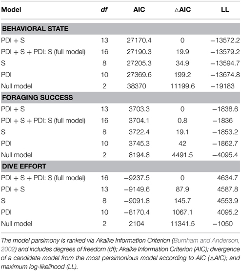
Table 1. Ranked model parsimony according to the significance of fixed effects (plankton density index—PDI; season—S) and their interaction term (PDI: S) in relation to each behavioral metric.

Behavioral Metrics in Response to Seasonal Plankton Densities

In the most parsimonious models (see Table 1) each behavioral metric exhibited by seals (i.e., behavioral state, dive effort and foraging success) was significantly correlated with plankton distribution, although dive effort was also influenced by season (Table 2). Linear mixed effect models indicated that both the search activity (i.e., behavioral state) and foraging success (i.e., mass gain rate), increased with plankton densities throughout the year (Figures 1, 2 respectively). Dive effort also increased with plankton densities, albeit a slightly stronger trend in winter and spring (Table 2, Figure 3). Dive effort was generally higher in summer compared with other times of the year (Table 2). A regression of the observed against the predicted values was positively significant for each model, but the model that included behavioral state had the lowest predictive capacity [F_(1,6398) = 1867.3, p < 0.0001, adj. R² = 0.23], followed by models that included foraging success [F_(1,5848) = 3010, p < 0.0001, adj. R² = 0.34] and dive effort [F_(1,6712) = 14268, p < 0.0001, adj. R² = 0.68] (see electronic Supplementary Material, Figure S1).

TABLE 2

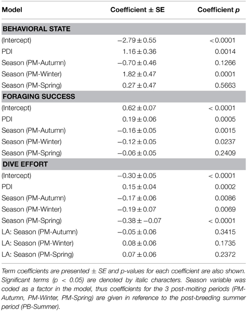
Table 2. Coefficients from our most parsimonious generalized mixed-effects models relating the plankton density index (PDI) to each behavioral metric (i.e., behavioral state, foraging success, dive effort).

FIGURE 1

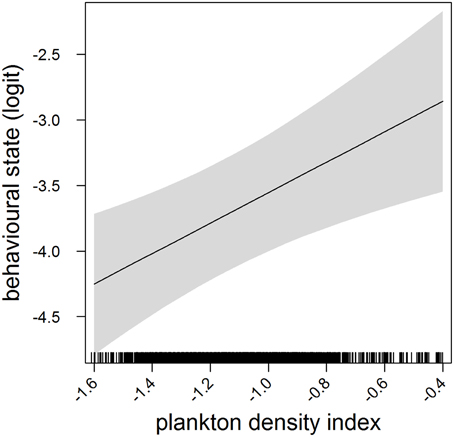
Figure 1. Effects plot of the relationship between plankton densities encountered by seals (i.e., PDI) and their behavioral state from our mixed model analysis. Shaded area indicates the confidence interval. Behavioral state has been logit transformed (higher values indicated an increasing likelihood of seals exhibiting horizontal search activity).

FIGURE 2

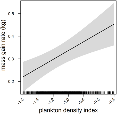
Figure 2. Effects plot of the relationship between plankton densities encountered by seals (i.e., PDI) and their foraging success (i.e., mass gain rate) from our mixed model analysis. Shaded area indicates the confidence interval.

FIGURE 3

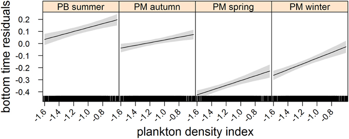
Figure 3. Effects plot of the relationship between plankton densities encountered by seals (i.e., PDI) and their dive effort (i.e., bottom time residuals) according to season from our mixed model analysis. Shaded area indicates the confidence interval.

Seasonal Spatio-Temporal Distribution

Predicted mass gain values from our foraging success model also showed that summer seal body condition improved with PDI at the distal end of the trip within the Polar Front Zone (PFZ), delineated by the sub-Antarctic front (SAF) and the southern Antarctic Circumpolar Current Front (SACCF), and generally north of East Antarctica (Figure 4). Both PDI and behavioral metric values generally peaked around December (summer) (Figure 5) at the greatest longitudinal (either ~140°E to the west or ~200–220°E to the east) and latitudinal (~63°S) extents attained by seals (Figure 6). In contrast, seals migrating during winter were largely south of the SACCF (>63°S) and shifted progressively eastward by the end of autumn through to spring (up to 240°E) along the maximum sea ice extent (Figures 4, 5). Predicted mass gain values show that body condition improved with PDI in pelagic waters between the SACCF and Ross Sea (~63°S–68°S) from late autumn to the end of winter (Figures 4B,C), which coincided with intensifying search activity during mid-winter (Figure 5B) as seals ended their eastward trajectory (Figure 6A) and slowly moved northward from between ~63°S and 68°S to between ~55°S and 68°S (Figure 6B). However, dive effort and PDI values had already declined in early March (Figures 5A,B respectively) as they began to pass south of the SACCF (Figure 6B; also see Figure 4B). By spring predicted mass gain rate in response to PDI dropped as their distribution shifted from these waters back toward MI as they returned to the island for the breeding season (Figure 4).

FIGURE 4

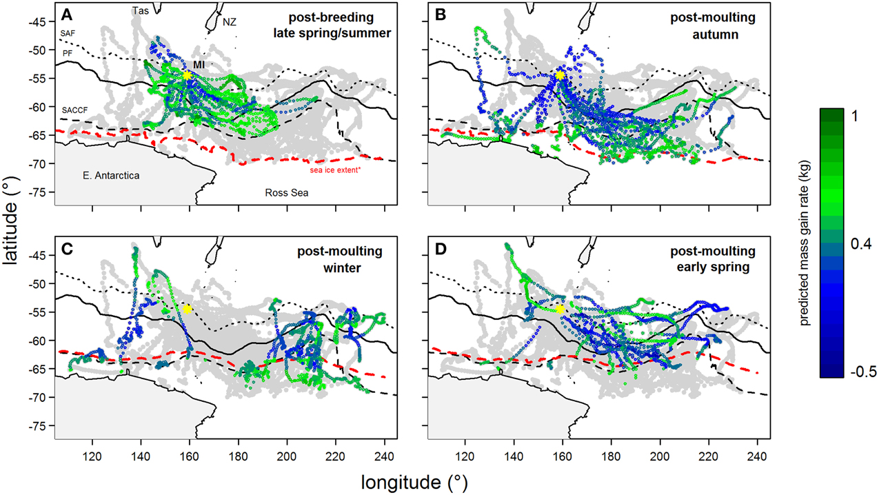
Figure 4. Tracks of southern elephant seals (from Macquarie Island) during their (A) summer and (B–D) winter foraging trips after the correction of geo-locations using state-space models (excluding locations in heavy sea ice). Year-round location points are light-gray and are overlaid with predicted mass gain values from our foraging success model (see legend for color code) according to season. Maps show the bottom of Tasmania (Tas) and New Zealand (NZ, top) and the coast of East Antarctica and Ross Sea (bottom). The yellow asterisk indicates Macquarie Island (MI). Three major fronts are also shown: sub-Antarctic Front (SAF—dotted); Polar Front (PF—solid); and Southern Antarctic Circumpolar Current Front (SACCF—dashed). The seasonal sea ice extent (red dashed line) is defined as the northern boundary where average sea ice concentration between 1999 and 2005 is >50%.

FIGURE 5

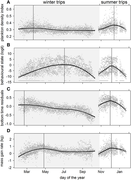
Figure 5. Seasonal trends over multiple years of (A) plankton densities encountered, (B) behavioral state, (C) dive effort, and (D) foraging success during the summer (non-shaded area) and winter (shaded area) foraging trips. Data values are represented by dark gray points. A locally-weighted polynomial regression smoother function applied to PDI and behavioral values using the R software package stats (function lowess; R Development Core Team, 2013). The loess fit and gray dashed lines represent the 95% confidence level. Vertical lines indicate the temporal peak for each measured metric.

FIGURE 6

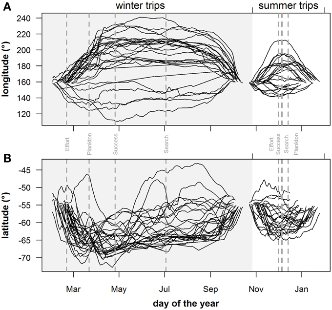
Figure 6. Geographical extent of individuals: seasonal trends of (A) longitude and (B) latitude position of individual seals during the summer (non-shaded area) and winter (shaded area) foraging trips. Gray vertical dashed lines in plots indicate peak values for plankton densities (Plankton), foraging behavior (Search), dive effort (Effort) and foraging success (Success).

Discussion

In the past it has been difficult to investigate the linkages between lower trophic levels and the foraging behavior of deep diving predators because concurrent data were often lacking, particularly in the polar regions. Resource distribution in relation to animal behavior is often estimated from satellite-derived chlorophyll-a (e.g., Guinet et al., 2001; Bradshaw et al., 2004; Suryan et al., 2012), but depth data are lacking. These data also become increasingly scarce and unreliable in polar regions due to cloud cover (Sumner et al., 2003), and are often spatially mismatched with animal behavior due to error inherent in animal location estimates (Ekstrom, 2004; Costa et al., 2010b). We provide an approach for investigating the trophic link between a deep diving predator and concurrent plankton densities in the 3D marine environment by using light data collected by sensors deployed on southern elephant seals (SESs). Integrated light attenuation in the top 250 m of the water column were used to infer year-round changes to plankton distribution in the Southern Ocean that followed known seasonal patterns in productivity. This is the first dataset (up to 50 SESs) used to examine how seal movement and feeding behavior respond to plankton and its seasonal variability in the Southern Ocean, providing rare evidence of regions of elevated plankton influencing seal foraging behavior. In addition, we demonstrate how the response of seals to resource structuring can give some insight into seasonal foraging strategies at high latitudes.

Seasonally-Contrasted Foraging Strategies in Relation to Resource Distribution

We hypothesized that the contrasting primary production between the spring-summer bloom and post-bloom period in winter required a fundamental change in elephant seal foraging strategy, but found no significant (or very little) seasonal differences. There were no pronounced seasonal differences in the influence of plankton densities on seal behavioral state or foraging success, albeit a small seasonal influence on dive effort. Seal search intensified and foraging success increased in response to elevated plankton densities not only in summer, but also during other times of the year including winter. This is despite the well-documented seasonal decline in phytoplankton biomass from the bloom period during early spring and summer to oligotrophic conditions during winter (Behrenfeld and Falkowski, 1997; Garibotti et al., 2005; Thomalla et al., 2011). These biological changes do not appear to affect the ability of seals to locate elevated plankton densities where prey availability increases. It is therefore likely that lower trophic aggregates are associated with seal prey either directly (feed on plankton) or indirectly (plankton reduce light penetration at depth, thereby improving seals' vertical access to prey (Guinet et al., 2014).

Marine resources are often heterogeneously distributed because of physical (e.g., eddy fields; d'Ovidio et al., 2013) and biological (e.g., grazing pressure; Hernández-León et al., 2008) processes (Begon et al., 2006). Optimal foraging theory predicts that animals will make decisions so as to maximize the net rate of energy intake while foraging in these patchy environments (Charnov, 1976). The different spatial distribution between summer and winter foraging trips may be a strategy for maximizing encounters with patches of prey. The summer seals intensified their search and dive effort at the distal end of their foraging trip where prey acquisition appeared to increase (according to foraging success). This coincided with known spring bloom events in deep pelagic waters between the major fronts of the Antarctic Circumpolar Current (ACC) (Sokolov and Rintoul, 2007; Sokolov, 2008), but not the blooms that often accompany the receding sea ice extent (e.g., Robins et al., 1995) (see Figure 4). This is perhaps because during their 2 month summer foraging trip less time is allocated for transit to favorable habitat compared with their much longer winter foraging trip; preferring instead to target blooms that are relatively close within the major fronts. We suspect a high degree of overlap between seal prey (mid-trophic level) and plankton (lower-trophic level) within these productive frontal regions during late spring and summer because the extent of phytoplankton biomass is so vast. Cotté et al. (2014) argue that the prey field may be relatively homogeneous and dense within a bloom in late spring/summer, and exhibit little spatial structure. We suggest that during the summer seals adopt a hierarchical foraging strategy by responding to large-scale biological cues during late spring/summer phytoplankton bloom periods in order to locate profitable prey fields at the smaller scale. These findings are consistent with Guinet et al. (2014) which showed summer seals (females) feeding during the day are more successful (indicated by prey capture attempts derived from accelerometer data) in areas where higher concentration of particles (indicted by the influence of plankton density on light attenuation) are encountered, but did not however consider females feeding in winter.

Despite oligotrophic winter waters the post-molting foraging trip remains vital for gestating females that must also build fat reserves for the up-coming breeding season. We revealed that winter seals, like summer seals, generally intensified their search, were likely to spend relatively more time foraging at depth, and exhibited increasing foraging success when encountering higher PDI. It is likely prey field distribution becomes increasingly patchy in space as productive waters from summer blooms become increasingly mixed with low-productive waters throughout the winter period (d'Ovidio et al., 2013; Cotté et al., 2014). We expect seals are encountering these increasingly isolated patches of productive waters as winter progresses. Cotté et al. (2014) have demonstrated how winter seals in transit along cold water filaments track water parcels originating from spring bloom patches as they are advected by the flow of the ACC. We suspect turning frequencies, and therefore periods of ARS, of the seals increased in winter in order to locate and follow these filaments. These filaments, which correspond to frontal transportation, are reported to carry high zooplankton densities (Labat et al., 2009; Perruche et al., 2011), which may explain why seals are more likely to increase search intensity in response to sites of elevated plankton densities, even throughout winter. Cotté et al. (2014) also suggest that seals may temporally exploit these rich filaments while also using them to track the most profitable meso-scale features where higher prey densities occur (e.g., eddies—Godo et al., 2012). This is consistent with our results which showed seals foraging in winter were more likely to spend greater time foraging at depth and increase foraging success in response to elevated plankton densities. Strong meandering meso-scale eddies created by the energetic ACC (Chelton et al., 2007) are thought to facilitate plankton accumulation (Godo et al., 2012) and retention times long enough to transfer energy to different trophic levels (Biggs, 1992; Riandey et al., 2005; Benitez-Nelson and McGillicuddy, 2008), including fish (e.g., Nishimoto and Washburn, 2002; Zainuddin et al., 2006) and apex predators such as SESs (d'Ovidio et al., 2013). These advected water parcels are thought to sustain the pelagic ecosystem east of its origin and could explain the progressively eastward displacement of winter foraging seals. Elephant seals are known to feed opportunistically even while in transit to winter forging grounds (Thums et al., 2011). Continuous foraging during transit has previously been reported in several other pelagic predators that feed over extensive regions, including wandering albatross Diomedea exulans (Weimerskirch et al., 2005), leatherback turtles Dermochelys coriacea (Hays et al., 2006), southern bluefin tuna Thunnus maccoyii (Bestley et al., 2010). This foraging strategy allows animals to efficiently locate highly dispersed prey items or isolated patches of prey (Sims et al., 2006) while still making progress to know areas of higher prey abundance.

By combining information from predator behavior and a concurrent plankton index (inferred from light measurements) we have developed a tool for describing the relationship between predators and biological activity in space and time, something which is crucial for understanding trophic links in the 3D marine environment. Because deep diving predators feed at depth future work will include separating sub-surface plankton (Guinet et al., 2013) distribution from surface values and comparing this information with predator foraging behavior. It will also be important to test our findings at a finer resolution to see if these trends persist at the dive scale or whether seals are only responding to large scale features that coincide with elevated plankton densities (e.g., summer phytoplankton plumes, mesoscale eddies). Nonetheless, our results provide some insight into the possible foraging strategies used by a marine predator in response to different resource distributions between summer and winter.

Conflict of Interest Statement

The authors declare that the research was conducted in the absence of any commercial or financial relationships that could be construed as a potential conflict of interest.

Acknowledgments

This research was supported in part by US Office of Naval Research grants N00014-10-1-0516 and N00014-12-1-0286 to Duke University and to the University of St Andrews. This work benefited from discussions with participants in a working group supported by Office of Naval Research grants N00014-09-1-0896 to the University of California, Santa Barbara and N00014-12-1-0274 to the University of California, Davis. Funding was also received from the MASTS pooling initiative (The Marine Alliance for Science and Technology for Scotland) and their support is gratefully acknowledged. MASTS is funded by the Scottish Funding Council (grant reference HR09011) and contributing institutions. We thank Michele Thums, Steve Wall and Corey Bradshaw for field assistance. We thank the Australian Antarctic Division for providing logistical support. We also thank Karine Heerah for her useful comments.

Supplementary Material

The Supplementary Material for this article can be found online at: http://www.frontiersin.org/journal/10.3389/fmars.2015.00021/abstract

References

Arrigo, K. R., van Dijken, G. L., and Bushinsky, S. (2008). Primary production in the Southern Ocean, 1997–2006. J. Geophys. Res. C Oceans 113:C08004. doi: 10.1029/2007JC004551