Individual-level Variation and Higher-level Interpretations of Space Use in Wide-ranging Species: An Albatross Case Study of Sampling Effects

Gutowsky, Sarah E.; Leonard, Marty L.; Conners, Melinda G.; Shaffer, Scott A.; Jonsen, Ian D.

doi:10.3389/fmars.2015.00093

ORIGINAL RESEARCH article

Front. Mar. Sci., 12 November 2015

Sec. Marine Megafauna

Volume 2 - 2015 | https://doi.org/10.3389/fmars.2015.00093

Individual-level Variation and Higher-level Interpretations of Space Use in Wide-ranging Species: An Albatross Case Study of Sampling Effects

$\r\nSarah E. Gutowsky*$ Sarah E. Gutowsky¹^*

¹Department of Biology, Life Sciences Centre, Dalhousie University, Halifax, NS, Canada
²Department of Ocean Sciences, University of California Santa Cruz, Santa Cruz, CA, USA
³Institute of Marine Sciences, University of California Santa Cruz, Santa Cruz, CA, USA
⁴Department of Biological Sciences, San Jose State University, San Jose, CA, USA
⁵Department of Biological Sciences, Macquarie University, Sydney, NSW, Australia

Marine ecologists and managers need to know the spatial extent of at-sea areas most frequented by the groups of wildlife they study or manage. Defining group-specific ranges and distributions (i.e., space use at the level of species, population, age-class, etc.) can help to identify the source or severity of common or distinct threats among different at-risk groups. In biologging studies, this is accomplished by estimating the space use of a group based on a sample of tracked individuals. A major assumption of these studies is consistency in individual movements among members of a group. The implications of scaling up individual-level tracking data to infer higher-level spatial patterns for groups (i.e., size and extent of areas used, overlap or segregation among groups) is not well documented for wide-ranging pelagic species with high potential for individual variation in space use. We present a case study exploring the effects of sampling (i.e., number and identity of individuals contributing to an analysis) on defining group-specific space use with year-round multi-colony tracking data from two highly vagile species, Laysan (Phoebastria immutabilis) and black-footed (P. nigripes) albatrosses. The results clearly demonstrate that caution is warranted when defining space use for a specific species-colony-period group based on datasets of small, intermediate, or relatively large sample sizes (ranging from n = 3–42 tracked individuals) due to a high degree of individual-level variation in movements. Overall, we provide further support to the recommendation that biologging studies aiming to define higher-level patterns in space use exercise restraint in the scope of inference, particularly when pooled Kernel Density Estimation (KDE) techniques are applied to small datasets for wide-ranging species. Transparent reporting in respect to the potential limitations of the data can in turn better inform both biological interpretations and science-based management decisions.

Introduction

A common goal in spatial ecology research or conservation planning is to identify the areas most frequented by a target group of free-ranging animals. In marine systems, this often involves identifying important areas beyond the shoreline, creating unique challenges for species that range widely across the open sea. Groups of interest for marine spatial planning could include for example specific community-level functional groups (e.g., apex predators, Block et al., 2011), taxonomic groups (e.g., seabirds, Ronconi et al., 2012), species-at-risk (e.g., African penguins Spheniscus demersus, Ludynia et al., 2012), sub-populations (e.g., seabird colonies, Louzao et al., 2011; sea turtle breeding areas, Schofield et al., 2013) or specific life history phases, often divided further by sex (e.g., pupping female white sharks Carcharodon carcharias, Domeier and Nasby-Lucas, 2013). Our ability to study the space use of marine animals belonging to a specific group of-concern continues to expand with innovations in animal-attached biologging devices that record location and other ancillary data (Cooke, 2008; Hussey et al., 2015; Wilson et al., 2015). Importantly, how we use these individual-based data to define space use more broadly for the higher-level group to which the tracked animals belong, influences how we interpret the biological and management implications of the findings.

For seabirds, individual-based tracking data are commonly used to infer higher-level interpretations of space use. The distant separation between terrestrial breeding and marine foraging areas requires the use of biologging devices to gain insights into habitat use at sea. Because extinction now threatens over 30% of extant seabird species (IUCN, 2015), a priority in conservation planning is to assess the variability and extent of the at-sea areas most frequented by birds (Croxall et al., 2012; Ronconi et al., 2012). Seabirds are generally seasonally colonial and migratory, thus specific regions are more heavily visited during different periods of their annual cycle. Defining period-specific space use can help to identify the source or severity of common or distinct threats posed at different periods in the annual cycle for a species, and for further sub-groups divided by for example age-class (e.g., Péron and Grémillet, 2013; Riotte-Lambert and Weimerskirch, 2013; Gutowsky et al., 2014a), or sex (e.g., Phillips et al., 2004; Hedd et al., 2014). At the colony level, individual-based tracking data have been used to discern period- and colony-specific space use and potential associated impacts for population dynamics for a variety of seabird species (e.g., Young et al., 2009; Catry et al., 2011; Gaston et al., 2011; Wakefield et al., 2011; Frederiksen et al., 2012; McFarlane Tranquilla et al., 2013).

Various analytical approaches are available to estimate home ranges (i.e., full extent of the area used) and utilization distributions (i.e., areas of concentrated space use within the range) from biologger-derived location data (Fieberg and Börger, 2012). Kernel Density Estimation (KDE) remains one of the most common tools for visualizing and quantifying animal ranges and distributions since its inception in ecological studies (Worton, 1989). KDE is a non-parametric statistical method for estimating probability densities. When applied to tracking data, the result of a KDE analysis is the creation of contours representing densities or intensities of space use, often called a Kernel Density Estimate (herein we use “KDE” interchangeably to refer to both the analytical approach and output of the analysis). There has been much discussion over best practices in implementing and reporting for KDE and other similar approaches, and these have been thoroughly reviewed elsewhere (e.g., Laver and Kelly, 2008; Kie et al., 2010; Fieberg and Börger, 2012; Fleming et al., 2015; Signer et al., 2015). Despite shifting baselines in execution, KDE continues to endure among ecologists as a relatively simple and accessible tool for describing space use.

Generally, the results of independent KDE for each tracked individual in a dataset are reported, thus facilitating comparisons among individuals in the extent and locations of home ranges and areas of high use. Generalizations are often made for the higher-level group to which the tracked individuals belong by reporting results across individuals (Laver and Kelly, 2008). However, within the seabird literature, location data from multiple individuals are often combined into a single pooled KDE analysis to describe space use without discriminating among individuals. The results are then used to extrapolate space use to the higher-level group to which the tracked individuals belong (e.g., species-colony-period specific). Wood et al. (2000) were among the first to recommend pooled KDE as a tool to define and compare space use between groups of seabirds based on group-level sets of KDE contours (two albatross spp. from the same colony during breeding), and the practice has since become commonplace. Some recent examples include the use of pooled KDE to compare space use between different annual periods for a species and colony (e.g., Robertson et al., 2014), different species from the same colony (e.g., Linnebjerg et al., 2013), different colonies of the same species (e.g., Young et al., 2009; Thiebot et al., 2011), and different species and colonies (e.g., McFarlane Tranquilla et al., 2013, 2015; Ratcliffe et al., 2014).

Scaling up individual-level location data in a pooled analysis to infer higher-level group spatial patterns has two related consequences: (1) the output masks the degree of variation in movements among the individuals in the dataset contributing to the analysis, and (2) it assumes tracked individuals reasonably represent the larger group as a whole. Individual-level space use is rarely reported together with group-level pooled analyses, unintentionally inhibiting assessment of the contribution of individuals to the observed higher-level spatial patterns. The assumption of representativeness is sometimes briefly conceded, but implications for the biological interpretations of the results generally are not formally evaluated. A number of marine vertebrate studies have illustrated an asymptotic saturation effect of increasing the number of tracked individuals or number of foraging trips per individual on estimates of the size of the area occupied by a sample of tracked animals in a pooled analysis (e.g., Wood et al., 2000; Hindell et al., 2003; Taylor et al., 2004; Breed et al., 2006; Soanes et al., 2013; Orben et al., 2015). These studies suggest that a sample of individuals may be representative of their respective group if the estimated occupied areas reach an asymptote before the maximum sample size is included in the analysis. In addition to the estimated size of the area occupied by a group, it has also been demonstrated that the geographic locations of contours resulting from pooled analyses of different individuals can vary depending on the degree of individual variation within the sample (Taylor et al., 2004; Breed et al., 2006; Orben et al., 2015). Beyond these few examples which directly address assumptions of group-level representativeness of a sample, consistencies in movements among individuals comprising a dataset and among members of the higher-level group they represent remain un-tested assumptions, especially in seabird studies with small sample sizes (Soanes et al., 2013).

Importantly, this oversight persists despite a number of published works recommending that biologists using biologging technologies exercise restraint in the inferential scope of the findings (Lindberg and Walker, 2007; Hebblewhite and Haydon, 2010). Here, we explicitly demonstrate the impacts of individual variation and sample size on inter-colony comparisons of space use (i.e., differences in the size of areas used, overlap or segregation in distributions) in relation to the stage of the annual cycle in two highly vagile seabirds, Laysan and black-footed (P. nigripes) albatross. Past work has used sub-sampling routines to identify the presence of an area asymptote as justification for pooled analyses. We use a similar approach but focus rather on the range in output at different sample sizes to assess the potential for sampling effects from individual-level variation on higher-level interpretations of space use. When not at the breeding colonies, Laysan and black-footed albatross inhabit the vast open waters of the North Pacific Ocean basin. Like many seabirds, a variety of anthropogenic threats have resulted in both species being listed as “Near Threatened” (IUCN, 2015), thus identifying at-sea habitat and spatial overlap with risks has been a management priority (Naughton et al., 2007; Arata et al., 2009). We expect our practical demonstration of the consequences of sampling effects to provide further insights into the importance of considering the inferential limitations of small datasets, for these and other wide-ranging species, especially when informing science-based conservation planning strategies and management decisions.

Methods

Logger Deployment

Fieldwork was conducted between 2008 and 2013 at two colonies in the Northwest Hawaiian Islands: Sand Island, Midway Atoll National Wildlife Refuge (28.21°N, 177.36°W; herein “Midway”) and Tern Island, French Frigate Shoals (23.87°N, 166.28°W; herein “Tern”). These breeding sites are located 1200 km apart with population sizes (including all islands within the atolls) for Laysan albatross (herein “Laysans”) of 408,130 breeding pairs at Midway and 3230 pairs at Tern, and for black-footed albatross (herein “black-footeds”) of 21,830 pairs at Midway and 4260 pairs at Tern (Arata et al., 2009). We deployed and recovered two types of leg-mounted global location sensing (GLS) loggers using similar approaches across device types, colonies, and species (Table 1). Breeding birds (generally of unknown sex and only one member of a pair) were selected and captured opportunistically at the nest during incubation or chick brooding for device deployment and recaptured for device retrieval in a subsequent breeding season. All devices were mounted to a plastic leg band using cable ties and marine grade quick-setting epoxy and attached to the tarsus (logger+attachment c. 5–9 g, <1% body mass; well below the recommended limit for albatrosses, Phillips et al., 2003). GLS recovery rates varied among years but were on average 77% at Midway (2008–2013) and 91% at Tern (2008–2010). While it was not possible to formally assess tag effects, deployments at a Laysan albatross colony on Oahu, Hawaii resulted in no detectable short-term effects on reproductive success (Young et al., 2009). The Institutional Animal Care and Use Committee at the University of California Santa Cruz approved all protocols employed in this study. Permission to carry out research on Midway and Tern was granted from The Hawaiian Islands National Wildlife Refuge, US Fish and Wildlife Service, Department of the Interior (although opinions expressed in this publication do not necessarily reflect those of the agency).

TABLE 1

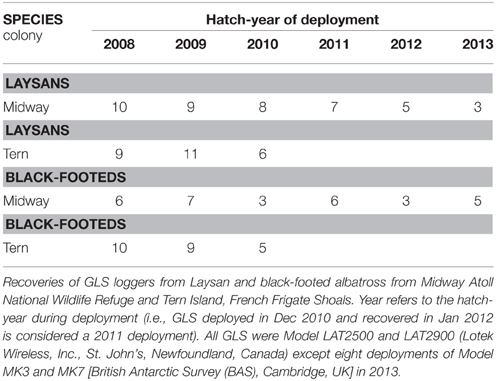
Table 1. Number of individual GLS tracks used in analyses by species-colony-year.

Positional Data Processing

GLS were programmed to record ambient light level data sub-sampled to maximums at 10-min intervals. Time of sunrise and sunset, estimated from thresholds of light level intensity, allowed for daily estimation of latitude from day length, and longitude from the time of local noon/midnight. Light data from BAS GLS were processed manually using TransEdit and Birdtrack software and light data from Lotek GLS were processed internally by automated template fitting software. The accuracy of latitude estimates during equinox periods is unavoidably compromised, as day length depends only weakly on latitude at this time (Ekstrom, 2004). For this study, locations on 15 days of either side of the equinoxes were excluded based on consistently suspect latitude estimates. All remaining locations were then processed using hierarchical state-space models (SSMs) estimated with Bayesian techniques (Jonsen et al., 2005; Block et al., 2011; Winship et al., 2012) to improve estimate accuracy and consistency across colonies and device types and to avoid unnecessary data loss (for SSM details see Gutowsky et al., 2014b).

We divided daily locations into four periods of the annual cycle approximately overlapping different life history phases (phenology can vary between species and colonies by c. 1–2 weeks) for subsequent analyses (Figure 1). Each period is 60 days in length thus avoiding overlap with the equinoxes (01-Mar–15-Apr and 01-Sep–15-Oct) and avoiding intervals of most intensive logger deployment and recovery wherein each individual bird's deployment length varied most (15-Dec–01-Jan). Locations within each period for each bird were included only if an individual contributed >30 days of data within that period to ensure each individual exhibited a range of natural behaviors for each life history phase (i.e., capturing time spent both at the colony and foraging at sea during the breeding season periods).

FIGURE 1

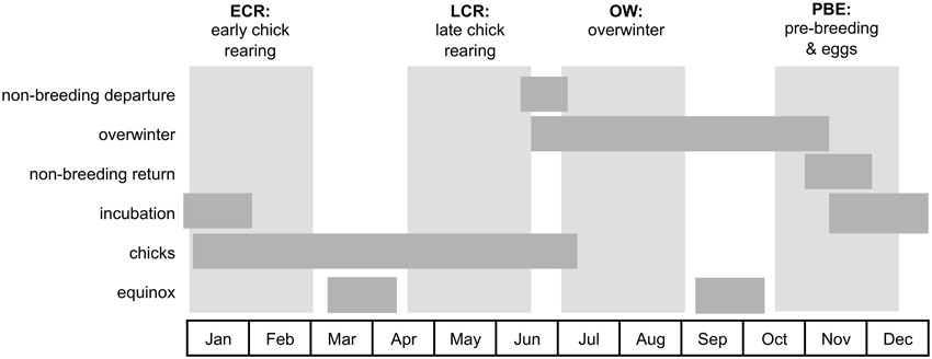
Figure 1. The four periods of the annual cycle considered in analyses. Daily GLS locations of Laysan and black-footed albatross were divided into four 60-day periods (vertical light gray blocks) associated with different life history phases (horizontal dark gray bars). Early chick rearing (ECR) coincides with late incubation, peak hatch, and early chick rearing (01-Jan to 01-Mar). Late chick rearing (LCR) coincides with the end of chick rearing (05-Apr to 15-Jun). Overwinter (OW) occurs during the non-breeding season, when all birds have departed the colonies and are at overwintering areas at sea (01-Jul to 01-Sep). Pre-breeding and eggs (PBE) encompasses the end of non-breeding, the return of birds to the colonies for courtship, and the transition into egg laying and incubation (15-Oct to 15-Dec). The timing of reproductive events were derived from Arata et al. (2009) and Gutowsky et al. (2014b) and typically varies little among colonies or between species (at most by c. 2 weeks). Each period avoids overlap with the equinoxes and intervals of most intensive logger deployment and recovery (15-Dec to 01-Jan).

We examined patterns of at-sea distribution within species between colonies for each annual period with KDE (Worton, 1989; Wood et al., 2000; Laver and Kelly, 2008; Kie et al., 2010), using purpose-built software written in Matlab (MathWorks Inc, USA; IKNOS Toolbox, Y. Tremblay unpublished). Limited sample sizes within years inhibited inter-annual comparisons due to the inability to differentiate among individual variation and true annual effects. Therefore, data were pooled across years within each period by colony and species. KDEs were conducted independently for each individual and as pooled KDEs where all locations from individuals within a species-colony-period dataset are pooled together for the analysis.

A KDE for bivariate data is defined as:

\begin{array}{l} f (x) = [1 ∕ (n h^{2})] \sum_{i = 1}^{n} K {\frac{(x - X_{i})}{h}} \end{array}

where X_i(i = 1, 2, …, n) is the sample of n observed locations (i.e., a coordinate vector of longitude and latitude) from a distribution with unknown density f, x is the location where the function is evaluated, h > 0 is the smoothing parameter (or bandwidth; details below), and K is a kernel density (we use a biweight kernel, as described in Seaman and Powell, 1996). The KDE method essentially places a kernel over each observed location in the dataset of sample size n, where X_i as the i^th observation. A grid is superimposed over the data and the function is evaluated at each grid intersection, or x (we computed KDEs on a 0.25° × 0.25° grid), providing a two-dimensional (bivariate) Gaussian density estimate for each x. The density estimated for each grid intersection represents an average density of all the kernels that overlap that location. Observations closer to the intersection contribute more to the estimate than those further away. The density surface can then be converted into contours of concentric polygons by connecting areas of equal density. Following the standard for most KDE studies (Laver and Kelly, 2008), we took the 50% kernel contour to represent regions of high use for each sample of individuals or individual, and the 95% kernel contour to represent the outermost limits of the range. The contours can then be visualized as distribution maps.

The most important decision in computing KDEs is the selection of the smoothing parameter, h (Kie, 2013). The value of h influences both the outermost limits of an estimated range, and the shape and distribution of the regions of high use (Kie et al., 2010); high values of h can lead to over-smoothing the kernel contours (i.e., contours contain fewer more contiguous polygons, considered lower precision with higher bias toward larger areas) while low values of h can under-smooth the kernel contours (i.e., contours break into smaller disjointed polygons, considered higher precision with bias toward smaller areas). The influence of h changes with the sample size of a dataset, where a higher number of locations contributing to an analysis will have lower optimal values of h for minimizing under- and over-smoothing (Kie et al., 2010). Because each species-colony-period dataset differed in sample size (including locations from six to 42 individuals in pooled KDEs), we selected h independently for each dataset using an automated data-based selection method to estimate optimal values for h (Sheather and Jones, 1991; Sheather, 2004). A second decision in calculating kernel contours is whether to hold h constant for all evaluated points (fixed kernels) or to allow h to vary as a function of local densities (local kernels, Kie, 2013). Local kernels increase h at points with lower location densities allowing for greater smoothing in areas with more uncertainty (Worton, 1989). With local kernels, smaller datasets comprised of fewer location estimates are subject to increased smoothing and less reliable contours overall relative to larger datasets, especially at the peripheries of the range (>80% kernel contours; Seaman et al., 1999). Because we are interested in comparing both the 50% and 95% kernel contours of KDEs generated from datasets of different size, we used a fixed kernel approach for our analyses. KDE iterations in our analyses resulted in optimized fixed h values for each dataset ranging from 0.0043–0.0738° latitude and 0.0038–0.119° longitude (mean ± standard deviation 0.0282 ± 0.01° latitude and 0.0385 ± 0.02° longitude).

Sampling Effects

We performed four period-specific independent KDEs for each individual, as well as a pooled KDE for each complete species-colony-period dataset. As a first assessment of the potential influence of individual-level variation on perceived higher-level space use from pooled KDE, we consider the effect of excluding a single individual on KDE output from each full species-colony-period dataset. We performed a pooled KDE (as outlined above) for iterations of max n–1 individuals (sequentially excluding each individual once, for a total number of iterations equal to max n), and recorded the area and geographic location of the resulting kernel contours. To represent the geographic location of pooled KDE kernel contours, we assessed the maximum and minimum latitudes and longitudes of the 95 and 50% contours. Because each set of kernel contour polygons can comprise multiple variably shaped polygons, it was not practical to compare the location of polygon centroids between pooled KDE iterations. The peripheral limits of the contours provide a generalization of the location of each group of polygons.

We also used a simple sub-sampling approach to assess the influences of different n and identity of the individuals comprising the sample on the output of pooled KDE for each species-colony-period dataset. Our approach is similar to previous studies (Wood et al., 2000; Hindell et al., 2003; Taylor et al., 2004; Breed et al., 2006; Soanes et al., 2013; Orben et al., 2015) but our focus is not identifying the presence of an asymptote but rather the range in output at each sample size. For each dataset, we randomly sub-sampled n individuals (without replacement) beginning with n = 3 and increasing in increments of two, up to three less than the maximum number available. For each value of n, we repeated the random selection process 100 times, resulting in 100 unique sub-samples of individuals for each n. We then carried out a pooled KDE generated from the daily locations of each sub-sample of individuals. The value of h for each KDE was again determined based on the data within each sub-sample. This approach most accurately simulates having only the data in the sub-sample from which to estimate the range and distribution of the represented group (i.e., the species and colony in a given period of the annual cycle). This differs from past studies, where a pre-determined fixed value of h was applied to all KDE iterations (e.g., Breed et al., 2006; Orben et al., 2015). Here we are interested in the degree of variation among KDE outputs given the “available” data set, and therefore a data-based selection method for each independent KDE is most appropriate. For each KDE, we recorded the total area of the resulting 95 and 50% kernel contours. We visualized the influence of n on the kernel contour areas by plotting the results of each set of 100 KDE iterations for a given value of n [as median, interquartile range (IQR, 50% of iterations around the median), whiskers to 1.5xIQR, and outlying data points indicating the maximum and minimum estimates for each n].

Results

Assessing Individual-level Variation within a Dataset

The results of independent KDE for each bird show differing degrees of variation in space use among the individuals tracked, depending on the species-colony-period dataset (Table 2; Figures 2, 3). Stacked individual 50% kernel contours visualize variation in geographic locations used by all individuals in a dataset, as well as the areas of most intense overlap among individuals. As one example, while independent 50% kernel contours for Laysans from Midway overlap most north and northwest of the colony during PBE, nine (of 42) tracked birds also exhibit 50% contours to the east, and northeast of the colony (Figure 2). During this period, individual Laysans from Midway occupied a mean 50% kernel contour area of 532,000 km², but this varied greatly among individual birds (±341,000 km² standard deviation, Table 2). The 95% kernel contour areas also varied greatly among individuals (6,624,000 ± 3,228,000 km², mean ± standard deviation; Table 2). Similarly, 50% kernel contours for black-footeds from Tern during OW occurred mostly along the coasts and offshore from British Columbia and Alaska, but four (of 24) tracked birds also occupied 50% kernel contours north and northwest of the colony over the open North Pacific (Figure 3). During this period, 50% kernel contours occupied a mean 149,000 km² (±149,000 km²) and 95% contours occupied a mean 2,001,000 km² (±1,526,000 km²).

TABLE 2

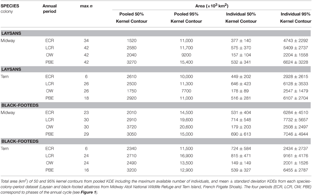
Table 2. Kernel contour areas from pooled and individual KDE analyses.

FIGURE 2

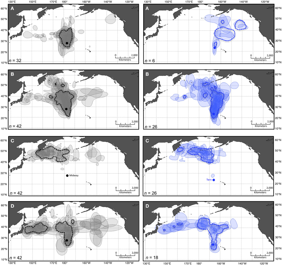
Figure 2. Pooled and stacked 50% kernel contours for two colonies of Laysan albatross during four periods of the annual cycle. Dashed polygons show 50% kernel contours from pooled KDE including GLS location data from all individual Laysan albatross tracked from Midway (left panes in gray) and Tern (right panes in blue) during four periods of the annual cycle: (A) ECR, (B) LCR, (C) OW, and (D) PBE (see Figure 1). Shaded polygons show 50% contours from individual KDE including data from each bird independently. The lightest shade indicates areas used by a single individual, and the darkest indicates areas of most intense overlap among individuals. Colonies are indicated in panels (C) by solid circles in their respective colors (projection: Lambert Cylindrical Equal Area, datum: WGS1984).

FIGURE 3

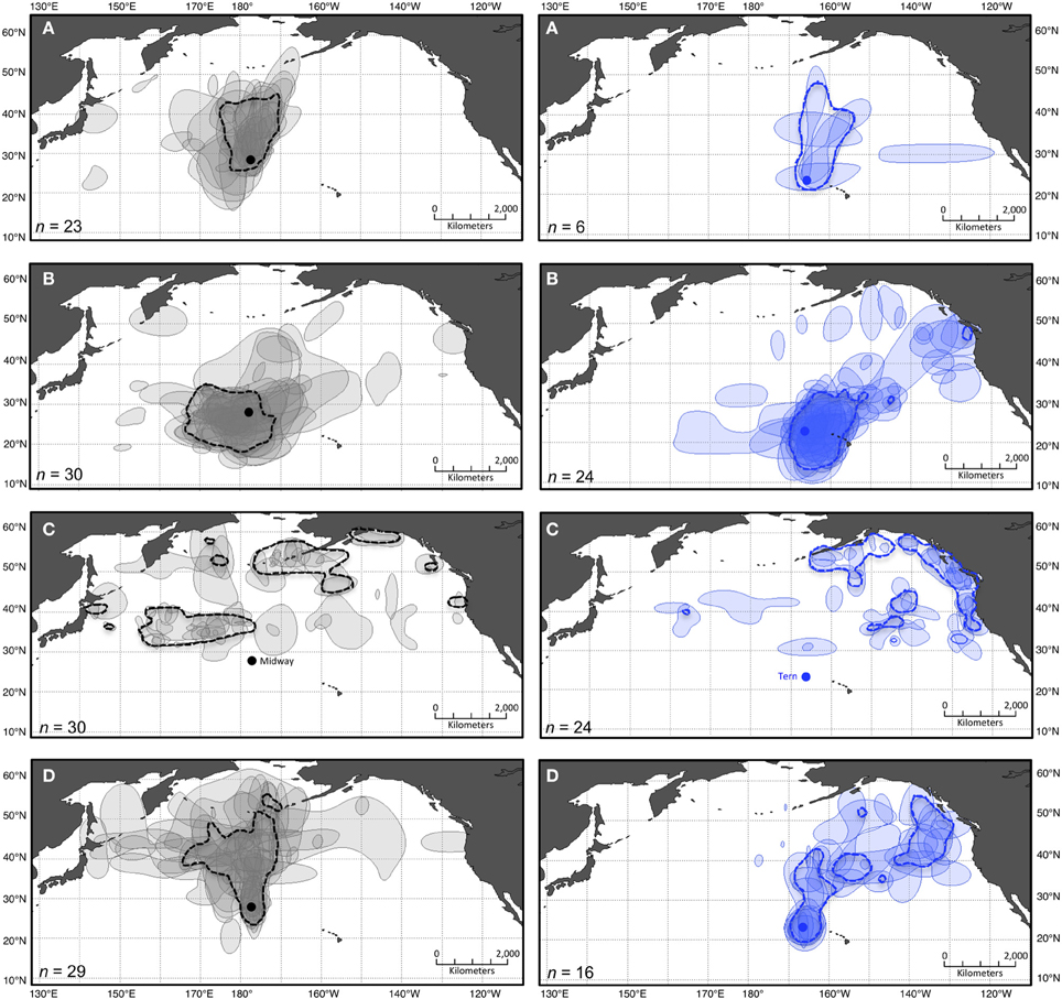
Figure 3. Pooled and stacked 50% kernel contours for two colonies of black-footed albatross during four periods of the annual cycle. Dashed polygons show 50% kernel contours from pooled KDE including GLS location data from all individual black-footed albatross tracked from Midway (left in gray) and Tern (right in blue) during four periods of the annual cycle: (A) ECR, (B) LCR, (C) OW, and (D) PBE (see Figure 1). Shaded polygons show 50% contours from individual KDE including data from each bird independently. The lightest shade indicates areas used by a single individual, and the darkest indicates areas of most intense overlap among individuals. Colonies are indicated in panels (C) by solid circles in their respective colors (projection: Lambert Cylindrical Equal Area, datum: WGS1984).

The results of layering pooled KDE generated from the maximum n for each dataset with independent stacked KDE indicate differing potential for misrepresentation of individual spatial diversity depending on the species-colony-period (Figures 2, 3). Generally, the 50% kernel contours resulting from pooled KDE including all locations in a dataset together fail to represent the extent of variability among individuals, both in geographic locations (Figures 2, 3) and size of areas used (Table 2). As one example, for black-footeds from Tern during LCR, 11 (of 23) individuals occupied 50% kernel contours along the northeast perimeter of the North Pacific ranging throughout offshore waters of Alaska to California, yet a pooled KDE identifies a group-level 50% kernel contour occupying a relatively small area near Vancouver Island, British Columbia (Figure 3). During this period, individual black-footeds used 50% kernel contour areas of 815,000 ± 471,000 km², while a pooled KDE indicates an overall area used of 2,710,000 km², masking the variation among individuals in the dataset (Table 2).

KDE outputs generated from iterations where single individuals are sequentially excluded from the analysis show variable sensitivity of pooled KDE to individual-level variation depending on the species-colony-period dataset (Tables 3, 4). For example, max n–1 sampling sensitivity during OW for both colonies was low for Laysans but high for black-footeds. For Laysans during OW, outputs from pooled max n–1 KDE were generally consistent in area and geographic location, suggesting that variation in movements among the individuals comprising the datasets from each colony during this period is relatively low (Tables 3, 4). Areas occupied by OW 50% contour estimates varied by 129,000 km² and 158,000 km², for Midway (max n = 42) and Tern (max n = 26), respectively (Table 3). For Midway Laysans, the locations of OW 50% contour estimates among max n–1 iterations were consistent (northern-most limits varying by only 0.66°N, western-most limits varying by 1.04°W; Table 4). Tern Laysans differed more in their east-west movements during OW, resulting in variable estimates of the western 50% contour limits (up to 5.93°W), while the northern limits were more consistent (ranging 0.38°N). For both colonies, estimates of the areas and geographic locations of the 95% contours followed similar patterns (Tables 3, 4). In contrast, black-footeds tracked from both colonies exhibited higher individual-level variation during OW than Laysans. Fifty percent contour area estimates from max n–1 pooled KDE iterations for both colonies varied ≥500,000 km² and 95% contour estimates varied >2,500,000 km² (Table 3). The northern limits of both 50 and 95% contour estimates varied by ≤ 2°N, but the western limits varied widely (Table 4). Western 50% contour limits were estimated across 5 and 2.64°W and 95% contour limits across 14.18 and 32.1°W (Midway and Tern, respectively; Table 4). The high individual-level variation in space use among black-footeds for both colonies during OW illustrated by independent KDEs (Figures 2, 3; Table 1) results in high variability in max n–1 pooled KDE outputs (Tables 3, 4).

TABLE 3

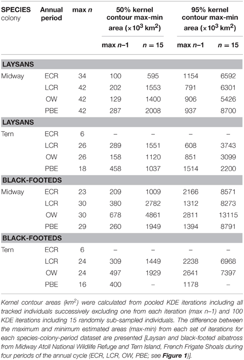
Table 3. Range in areas of 50 and 95% contours from pooled KDE with sample sizes of maximum n less one and n = 15.

TABLE 4

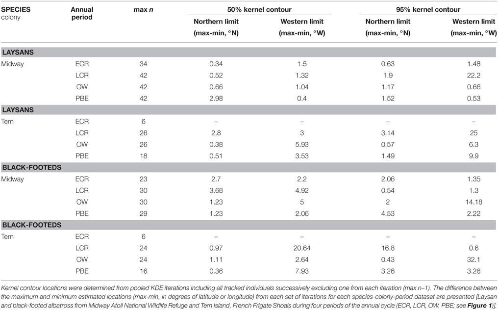
Table 4. Range in 50 and 95% contour locations from KDE successively removing one individual.

Sampling Sensitivity of Pooled KDE at Intermediate Sample Sizes

Pooled KDE iterations generated from the daily locations of 15 randomly selected individuals showed varying sensitivity of KDE output at intermediate values of n. The difference between the largest and smallest 50% contour estimated from KDE iterations of n = 15 ranged from 595,000 km² (Laysans from Midway during ECR) to 4,861,000 km² (black-footeds from Midway during OW; Table 3). The area of the 95% contour was similarly variable at n = 15; the difference between the largest and smallest estimated 95% contour was least for Laysans from Tern during PBE (2,200,000 km²) but this dataset had a small total number of individuals (max n = 18) from which to draw sub-samples. KDE iterations of n = 15 produced 95% contours varying in area generally between 3,000,000 and 9,000,000 km², but varied by as much as 13,115,000 km² for black-footeds from Midway during the OW period (Table 3).

The geographic location of the 50% contour was highly sensitive to sampling effects at n = 15. The outermost limits of 50% contours resultant from 100 unique KDEs of 15 randomly sub-sampled individuals varied widely depending on the species-colony-period considered (Figure 4). Fifty percent contours varied least in location during ECR, however this could only be assessed for Midway. During the remaining three annual periods, the limits of the 50% contour estimated from KDE iterations for both colonies of Laysans and black-footeds varied least in the southernmost extents (Figure 4). The high degree of variation in the northern-, eastern-, and western-most limits resulted in 50% contours spread widely across the North Pacific, yielding either high overlap or complete segregation among colony-specific ranges depending on the 15 individuals contributing to the KDE (Figure 4).

FIGURE 4

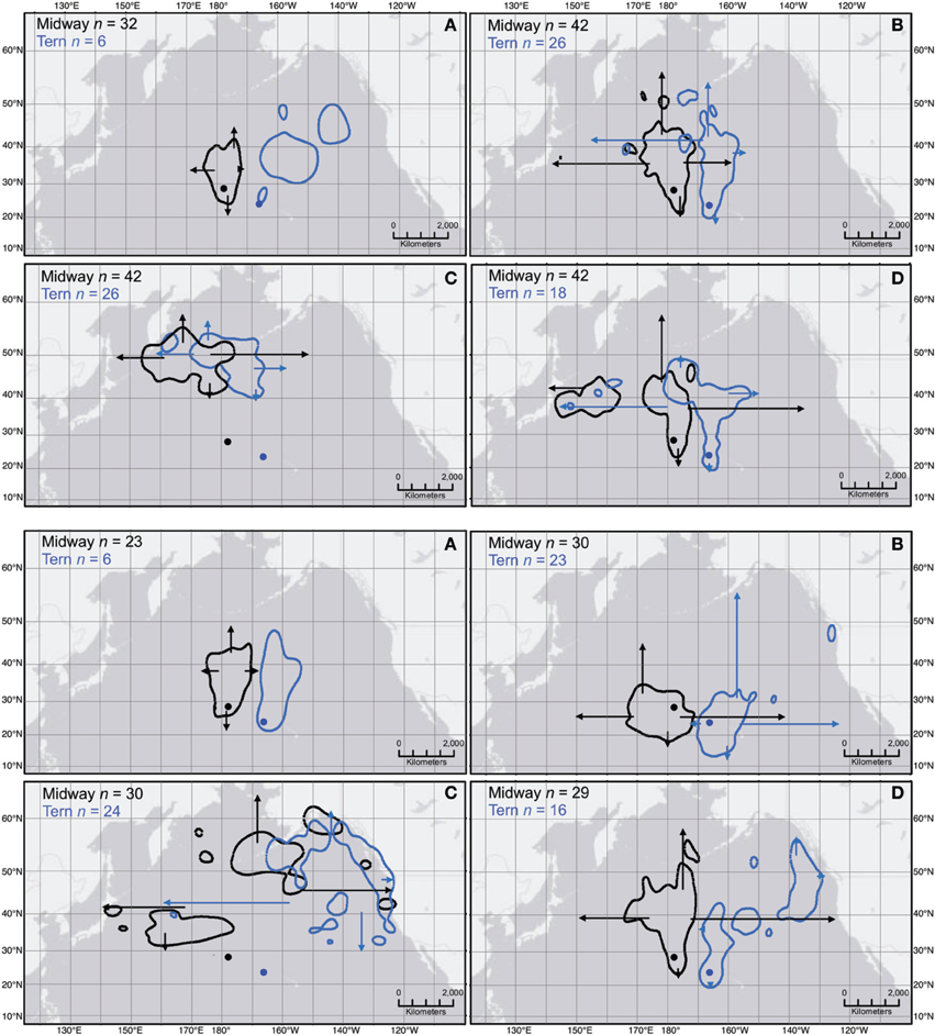
Figure 4. Sampling effects on the location of 50% kernel contours from pooled KDE for two colonies of Laysan and black-footed albatross during four periods of the annual cycle. Polygons show 50% kernel contour results from pooled KDE including GLS location data from all individual Laysan albatross (top four panes) and black-footed albatross (bottom four panes) from Midway and Tern (n shown in each pane). Arrows depict the outermost extents of 50% kernel contours (northern, eastern, southern, and western limits for each set of polygons) resulting from 100 KDE generated from the daily locations of 15 randomly selected individuals from the full dataset for each colony. The outermost perimeter of the 50% kernel contour from KDEs ranged between the beginning and end of each arrow in the four cardinal directions as shown. Each set of four panes represent the four periods of the annual cycle: (A) ECR, (B) LCR, (C) OW, and (D) PBE (see Figure 1). Colonies are indicated by solid circles in their respective colors (projection: World Azimuthal Equidistant, datum: WGS1984).

Sampling Sensitivity of Pooled KDE at Small Sample Sizes

Small values of n comprised of only a few individuals resulted in highly variable pooled KDE output (Figures 5, 6). Sub-samples of three to five random individuals consistently produced areas of 50 and 95% kernel contours that varied by a factor of three to four. For example, three randomly selected Laysans or black-footeds from Midway during PBE can produce a 95% contour encompassing an area anywhere from 5,000,000 to 20,000,000 km² (Figures 5, 6). Similarly, five randomly selected Laysans from Tern during OW can produce a 50% contour encompassing areas from 600,000 to 2,300,000 km² (Figure 6). The highest degree of spatial diversity among individuals occurred among black-footeds tracked from Tern during OW, where pooled KDE based on location data from five (of 24) individuals can result in 50% contours encompassing areas differing by a factor of eight (ranging from 400,000 to 3,200,000 km², Figure 6).

FIGURE 5

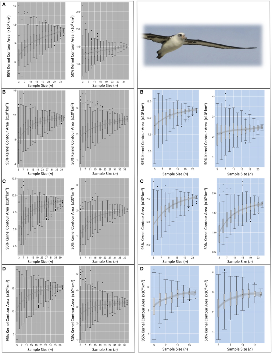
Figure 5. Pooled KDE contour areas for Laysan albatross from two colonies during four periods of the annual cycle. Pooled KDE contour area (km²) outputs for Laysan albatross from colonies at Midway (left panes in gray) and Tern (right panes in blue). Boxplots for each sample size (from n = 3 to n = max n–3) represent the 95 and 50% kernel contour areas of 100 iterations of KDE generated from the daily locations of n randomly selected individuals' GLS tracks. The final boxplot in each panel depicts the results of KDE iterations of max n–1 (i.e., removing one individual from the dataset for each KDE), resulting in max n number of total iterations. Each set of four panes represent the four periods of the annual cycle: (A) ECR (insufficient data for Tern), (B) LCR, (C) OW, and (D) PBE (see Figure 1). LOESS smoothers are for visual interpretation and should be used only as a guide.

FIGURE 6

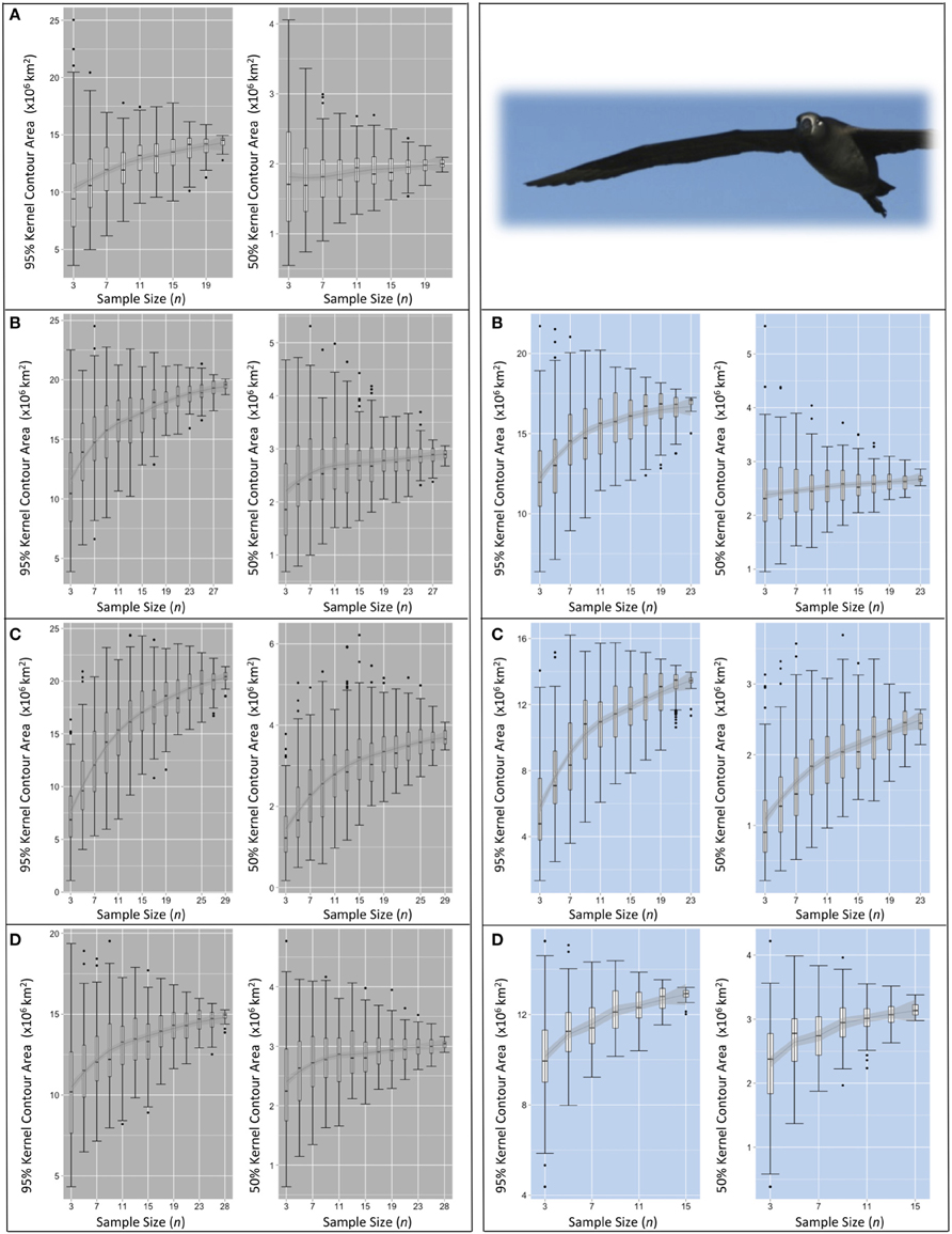
Figure 6. Pooled KDE contour areas for black-footed albatross from two colonies during four periods of the annual cycle. Pooled KDE contour area (km²) outputs for black-footed albatross from colonies at Midway (left panes in gray) and Tern (right panes in blue). Boxplots for each sample size (from n = 3 to n = max n–3) represent the 95 and 50% kernel contour areas of 100 iterations of KDE generated from the daily locations of n randomly selected individuals' GLS tracks. The final boxplot in each panel depicts the results of KDE iterations of max n–1 (i.e., removing one individual from the dataset for each KDE), resulting in max n number of total iterations. Each set of four panes represent the four periods of the annual cycle: (A) ECR (insufficient data for Tern), (B) LCR, (C) OW, and (D) PBE (see Figure 1). LOESS smoothers are for visual interpretation and should be used only as a guide.

The locations of contours were also highly sensitive to the sample of individuals at small values of n. Generally for both species and colonies during all annual periods, sub-samples of three to five random individuals produced 50 and 95% kernel contours that varied in their northern limit by at least 10° of latitude. Contours often varied in the northern limit by 20°, and up to 30° of latitude for the 95% contour representing black-footeds from Tern during LCR. The amount of variation among iterations at small n was generally similar regardless of the size of the full dataset from which sub-samples were drawn.

Sampling Effects with Increasing Sample Size

For species-colony-period datasets where the maximum n was >30 individuals, the sensitivity of pooled KDE in the resultant areas of 50 and 95% contours appears to stabilize with increasing n. The median areas of the contours roughly approach an asymptote between n = 17–21 (both species from Midway, Figures 5, 6). Around the same n, the area estimates resulting from each set of iterations encompass similar IQRs and maximum/minimum values. At this n, increasing the number of individuals contributing to a KDE does not appear to increase the probability of obtaining a more refined estimate of the amount of area occupied by a pooled estimate of the 50 or 95% kernel contour. However, the range in pooled KDE outputs for some species-colony-period datasets remains large even when sampling effects appear to reach saturation. For example, sub-samples of n = 31 individual Laysans from Midway during PBE result in 95% contour areas varying by 7,250,000 km² and 50% contour areas varying by 1,000,000 km², despite an apparent stabilization of median outputs around n = 17. As n approaches within five individuals of the max n, the variability among KDE area outputs predictably decreases, as the sub-samples are drawn from a finite pool of individuals and the results will inevitably become increasingly similar. Species-colony-period datasets with maximum n less than 30 individuals exhibited less consistently identifiable values of n at which sampling sensitivity for KDE area estimates stabilized (both species from Tern, Figures 5, 6). For these datasets, the estimated areas occupied by the 50 and 95% contours continue to increase or remain highly variable until n reaches within five individuals of max n.

Discussion

From our exploratory assessment of sampling effects, the number and selection of individual Laysan or black-footed albatrosses contributing location data to a pooled KDE had a marked effect on perceived spatial usage at the colony level for both species. Where an asymptotic saturation effect was detectable (datasets with maximum n > 30), a minimum of 17–21 individuals was required to minimize the variability among mean KDE outputs generated from sub-samples of individuals representing a higher-level group. Even when this minimum sample size is satisfied, the influence of inconsistencies among individual space use on higher-level interpretations is apparent when the full range in outputs at the saturation sample size is considered, along with independent individual-level KDE. Our analysis highlights some of the major limitations for biological interpretations based on different sample sizes that are not apparent from pooled KDE analyses alone. We discuss some examples of common individual-to-colony level extrapolations in seabird tracking research that could benefit from reporting and discussing the potential influence of individual variation.

Commonly in multi-colony tracking studies, the size of the areas used and the degree of at-sea spatial segregation among seabird colonies are delineated by a pooled KDE from a sample of tracked individuals from each group. The size of pooled KDE 50 or 95% contours are quantified and compared, and the degree of overlap between groups is calculated (e.g., Young et al., 2009; Frederiksen et al., 2012; Thiebot et al., 2012; McFarlane Tranquilla et al., 2013; Ratcliffe et al., 2014). However, without consideration of individual variation within an available dataset, these higher-level inferences can be inadvertently misleading. With a small number of tracked individuals (n = 3–15) of Laysans or black-footeds, our analysis shows that the calculated degree of overlap between contours taken to represent colony-specific ranges can vary between complete segregation and extensive overlap, dependent on the identity and number of individuals sampled. Predictably, sampling effects are strongest outside of the early chick rearing period (Figures 5, 6), a time when central place constraints are most limiting on the degree of individual variation in movements (Orians and Pearson, 1979).

Tracked individuals are sometimes used to estimate the proportional use or potential presence within specified regions and periods for birds from different colonies based on colony population size estimates. For black-legged kittiwakes (Frederiksen et al., 2012) and murres (Uria spp., McFarlane Tranquilla et al., 2013), the overwinter movements of tracked individuals have been taken to represent all of their colony members proportional to the colony's breeding population, thereby “distributing” members among specified regions of interest. Pooled KDE 50% contours generated from 15 or fewer individuals were taken to represent 11 of 16 kittiwake study colonies, and three of those colonies were represented by 5–7 tracked birds (Frederiksen et al., 2012). For example, seven birds from one colony represented the spatial distributions of c. 150,000 pairs nesting in the Newfoundland-Labrador Shelf Large Marine Ecosystem. From our case study, it is clear that colony-level inferences of space use based on seven individual Laysans and black-footeds from Midway and Tern would result in considerably different estimates of potential presence of birds from these colonies throughout the North Pacific depending on the identity of the individuals tracked. Further, if 15 individual black-footeds were taken to represent the overwinter range and distribution of the Midway colony, the area within which >21,000 pairs (>35% of the total breeding population, Arata et al., 2009) would be “distributed” could differ by as much as 13,000,000 km² (Table 3) and vary greatly in geographic location (Figure 4), depending on the individuals sampled.

Even a reasonably large sample size can result in a biased depiction of space use based on pooled KDE 50% kernel contours. Presenting the results of independent KDE for each of the 42 Laysans tracked from Midway during PBE illustrates how pooled KDE vastly under-represents the potential presence of the >400,000 pairs of Laysans nesting at Midway (c. 70% of the total breeding population, Arata et al., 2009) over the pelagic eastern North Pacific during this time (Figure 2). Similarly, pooled KDE for 18 Laysans tracked from Tern during PBE under-estimates the potential importance of the western North Pacific for birds from this small colony (Figure 2). The size of the pooled KDE 50% contour areas would be estimated around 3,000,000 km² for both colonies, but would differ greatly among the individuals tracked (Table 2). If pooled analyses from both colonies were used to “spatially distribute” Laysans throughout the North Pacific Ocean during PBE, an assessment of proportional use between the colonies based on our complete tracking datasets would be misguided. In past studies, authors have often acknowledged the assumption that the movements of sub-sampled birds are representative of all birds from each colony but the potential implications for the conclusions are not made explicit. Addressing sampling effects with a clear representation of individual variation within the datasets would help to ensure that management recommendations made are as reliable and useful as possible.

A straightforward approach to reporting individual variation in movement within a tracking dataset is to conduct and report individual-level analyses, as illustrated recently by Ceia et al. (2015), Young et al. (2015), and in the present study (Table 2; Figures 2, 3). While identifying the locations and areas of high use regions is more challenging to describe quantitatively from stacked individual contours, the degree of variation among individuals is clear. If group-level pooled analyses are still desirable, asking the simple question, “If we tracked one less individual, how different could the results of the pooled analysis be?” can be an effective means of considering whether a pooled analysis is appropriate for higher group-level inferences. As illustrated with our max n–1 analyses, exclusion of a single individual in some cases can have a significant influence on the group-level range and distributions estimated from a pooled KDE (Tables 3, 4), sending up a “red flag” for pooled analysis alone. For example, the east-west variation among the movements of Laysans tracked from both Midway (n = 42) and Tern (n = 26) during late chick rearing has a sizeable effect on the western-most limits of max n–1 pooled KDE 95% contours (Table 4). Taking the space use of these birds as representative of all members of their respective colony during this period would be ill advised. The convenience of a single pooled analysis to represent the space use of a group of individuals can come at the loss of important information on individual movements that can greatly impact higher-level biological inferences.

Importantly, the shape of area saturation curves alone do not fully disclose the influence of individuals on the output of pooled analyses, especially when the outputs are used to draw comparisons in space use among groups of interest. The variability among sub-samples should be assessed including maximum and minimum estimates in area occupied, along with the range in geographic locations of those areas. Increasingly, studies are including significance tests for overlap analyses; the proportional area of overlap between specified contours estimated for groups of interest from full datasets are compared with those estimated from randomized iterative sub-samples as a test of whether enough individuals were tracked to make reasonable higher-level inferences of significant spatial segregation (e.g., Breed et al., 2006; Kappes et al., 2011; Cleasby et al., 2015; Orben et al., 2015). This approach, coupled with area saturation curves, can improve confidence in the appropriateness of higher-level extrapolations. However, it is important these assessments are conducted for smaller contours (i.e., 50%) where individual variation has a much higher influence on pooled outputs (Figures 5, 6), and should be accompanied by reporting of individual-level analyses, especially where the size of datasets are limited.

Here we focus on KDE, but there are a variety of approaches for estimating group-specific ranges and the distribution of locations within that range (Kie et al., 2010). Grid cell methods offer a simple alternative, where the cumulative time spent within cells of a predefined grid size is used to identify the extent of a group's range and areas of most intense use (e.g., Soanes et al., 2013). Other methods take a habitat preference modeling approach, which takes into account environmental factors that shape patterns of space use (e.g., Aarts et al., 2008; Wakefield et al., 2011; Raymond et al., 2015). There have been a number of recent advances in approaches for estimating space use at the individual level which incorporate both the spatial and temporal nature of tracking data to estimate distribution contours, but most have not been expanded to generate group-level estimates of space use (e.g., Time Local Convex Hull, Lyons et al., 2013; Baker et al., 2015; movement-based KDE, Benhamou, 2011). Regardless of the approach selected as the best method to scale up individual location data to infer higher-level patterns in space use, the number and identity of the individuals contributing to the analysis has some effect on the output. The biases introduced from individual variation and sample size can be accounted for in part by methods that use mixed-effects modeling (e.g., Aarts et al., 2008). For other methods, like KDE or grid cells, the output of pooled analyses should be interpreted with careful consideration of the sensitivity to sampling effects, especially for wide-ranging species with high potential for individual-level variation in movements.

Location data can be obtained from a variety of tracking device types, varying in location uncertainty (Wakefield et al., 2009). Devices with higher uncertainty, such as GLS deployed on animals capable of traveling large daily distances, will inherently introduce more error in defining group-specific ranges, and distributions. SSM approaches offer a considerable advancement in refining location estimate uncertainty by incorporating device-specific error and movement dynamics into estimates of true daily positions (Jonsen et al., 2005; Winship et al., 2012). Still, the remaining uncertainty in our SSM-estimated locations was not accounted for in KDE (estimated as Bayesian 95% credible limits from the posterior distributions of individual location estimates, mean ± standard error, 0.89 ± 0.08° latitude and 0.92 ± 0.06° longitude). While small differences in geographic locations of contours may be attributable in part to underlying location estimate uncertainty, the large differences observed among sub-sampled KDE iterations for many species-colony-period KDEs likely reflect individual-level differences. Given the vast spatial scale at which our study species are acting and the magnitude of differences among KDE outputs, the effect of location uncertainty is not likely greater than the effect of true individual-level spatial diversity on the observed variation among pooled KDE output (particularly KDE of n = 15 random individuals; Table 3; Figure 4).

We are certainly not the first to caution that small sample sizes of biologger-tracked individuals increase the probability of erroneous higher-level conclusions (e.g., Lindberg and Walker, 2007; Hebblewhite and Haydon, 2010; Schofield et al., 2013; Soanes et al., 2013). Further, the examination of intra-population variation among individual movements is presently a burgeoning field in biologging studies of marine vertebrate behavior (reviewed by Patrick et al., 2014). Yet a major gap remains where inferences continue to be drawn from individual-based tracking data with insufficient consideration of the influence of sampling effects. Consistency among individuals in their movements will vary depending on a given species' biology, and the representativeness of a sample will also be a function of the total size of the represented group (Lindberg and Walker, 2007; Hebblewhite and Haydon, 2010). Sampling effects should be evaluated on a case-by-case basis. Many seabirds do not range widely from small colonies during the breeding season, for example, and colony-level interpretations of space-use may be entirely justified (e.g., Wakefield et al., 2013). During non-breeding, many migrate far from the colonies where colony members may or may not be consistent in their movements and overwinter areas most frequented. In some cases, it may simply be unreasonable to delineate the boundaries of group-specific distributions due to an inability to confidently infer higher-level patterns with the available sample of tracked individuals. As albatrosses may be an extreme example of wide-ranging pelagic seabirds, a comparative analysis similar to that presented here could be undertaken for species with differing degrees of individual variation and extent in movements throughout the annual cycle. In light of our results, we caution against drawing lines around group-specific ranges based on a sample of tracked individuals without first assessing and reporting potential sampling effects. This is especially true in calculating proportional areas of overlap and estimating “potential presence” between groups of interest (i.e., species, colonies, periods, age classes, sexes) based on substantial extrapolations from few tracked individuals.

Tracking data has a key role to play in developing management and recovery plans for seabird species-at-risk, and in the designation and monitoring of Marine Protected Areas, especially when integrated with a variety of different approaches (Croxall et al., 2012; Ronconi et al., 2012; Young et al., 2015). The effectiveness of advising conservation decisions based on the movements of individuals ultimately depends on the clarity with which we concede the limitations of the data and subsequent analyses. This is especially important for wide-ranging pelagic seabirds, as these families have experienced the largest documented population declines (Paleczny et al., 2015) and have high potential for individual variability in movements across the oceans they inhabit relative to shorter-ranging and coastal species. For most marine wildlife tracking studies, the number of individuals successfully tracked falls short of an “ideal” (i.e., statistically robust and biologically relevant) sample size. Rather, the ultimate sample size is governed by ethics, time, costs and recovery rates, where the final dataset can often unavoidably be comprised of location data from few individuals. As such, assessment and acknowledgement of the sensitivity of a chosen analytical approach to sampling effects at the available sample size need to become the norm, especially for higher-level interpretations of space use for wide-ranging marine species.

Conflict of Interest Statement

The authors declare that the research was conducted in the absence of any commercial or financial relationships that could be construed as a potential conflict of interest.

Acknowledgments

We thank the US Fish and Wildlife Service volunteers and staff for logistical and data collection support in the field. This study was supported by grants from the National Geographic Society Committee for Research and Exploration, NOAA Fisheries National Seabird Program, Gordon and Betty Moore Foundation, David and Lucile Packard Foundation, Alfred P. Sloan Foundation, National Ocean Partnership Program, Office of Naval Research, National Sciences and Engineering Research Council of Canada, Cooper Ornithological Society, and Society of Canadian Ornithologists.

Abbreviations

Laysans, Laysan albatross Phoebastria immutabilis; black-footeds, black-footed albatross Phoebastria nigripes; Midway, Midway Atoll National Wildlife Refuge, Northwest Hawaiian Islands; Tern, Tern Island, French Frigate Shoals, Northwest Hawaiian Islands; GLS, Global Location Sensing archival geolocator tag; ECR, Early chick rearing; LCR, Late chick rearing; OW, Overwinter; PBE, Pre-breeding, egg laying and incubation; KDE, Kernel Density Estimation or Estimate (used interchangeably).

References

Aarts, G., MacKenzie, M., McConnell, B., Fedak, M., and Matthiopoulos, J. (2008). Estimating space-use and habitat preference from wildlife telemetry data. Ecography 31, 140–160. doi: 10.1111/j.2007.0906-7590.05236.x