 Johan Schijf
 Shannon M. Burns
- 1Chesapeake Biological Laboratory, University of Maryland Center for Environmental Science, Solomons, MD, USA
- 2Department of Marine Sciences, University of Georgia, Athens, GA, USA
- 3College of Marine Science, University of South Florida, St. Petersburg, FL, USA
Electrochemical techniques like adsorptive cathodic stripping voltammetry with competitive ligand equilibration (ACSV-CLE) can determine total concentrations of marine organic ligands and their conditional binding constants for specific metals, but cannot identify them. Individual organic ligands, isolated from microbial cultures or biosynthesized through genomics, can be structurally characterized via NMR and tandem MS analysis, but this is tedious and time-consuming. A complementary approach is to compare known properties of natural ligands, particularly their conditional binding constants, with those of model organic ligands, measured under suitable conditions. Such comparisons cannot be meaningfully interpreted unless the side-reaction coefficient (SRC) of the model ligand in seawater is thoroughly evaluated. We conducted series of potentiometric titrations, in non-coordinating medium at seawater ionic strength (0.7 M NaClO4) over a range of metal:ligand molar ratios, to study complexation of the siderophore desferrioxamine B (DFOB) with Mg and Ca, for which it has the highest affinity among the major seasalt cations. From similar titrations of acetohydroxamic acid in the absence and presence of methanesulfonate (mesylate), it was determined that Mg and Ca binding to this common DFOB counter-ion is not strong enough to interfere with the DFOB titrations. Stability constants were measured for all DFOB complexes with Mg and Ca including, for the first time, the bidentate complexes. No evidence was found for Mg and Ca coordination with the DFOB terminal amine. From the improved DFOB speciation, we calculated five SRCs for each of the five (de)protonated forms of DFOB in trace-metal-free seawater, yet we also present a more convenient definition of a single SRC that allows adjustment of all DFOB stability constants to seawater conditions, no matter which of these forms is selected as the “component” (reference species). An example of Cd speciation in seawater containing DFOB illustrates the non-trivial use of different SRCs for polyprotic, polydentate organic ligands.
Introduction
Organic ligands dominate the solution speciation in seawater of many trace metals, notably Fe (Rue and Bruland, 1995), Co (Baars and Croot, 2015), Ni (van den Berg and Nimmo, 1987), Cu (Jacquot et al., 2013), Zn (Jakuba et al., 2012), Cd (Baars et al., 2014), and Pb (Capodaglio et al., 1998). Ligand concentrations and conditional stability constants can be measured for specific metals using electrochemical techniques (Pižeta et al., 2015), but the identity of these molecules remains largely unknown. Whereas for several metals a division has traditionally been made into a class of strong ligands (L1) and a more abundant class of weaker ligands (L2), based on the observed stability constants (Coale and Bruland, 1988), it has been argued that such divisions are an instrumental artifact and actually reflect a continuum of compounds spanning a broad window of metal affinities (Town and Filella, 2000). Evidence exists, particularly in coastal waters, for a prominent role in organic Fe and Cu complexation played by humic acids (Bundy et al., 2015; Whitby and van den Berg, 2015), an ill-defined assemblage of large, non-specific ligands that are refractory breakdown products of marine, or possibly terrestrial, organic matter.
Nonetheless, marine microbes doubtlessly make unique ligands to regulate the bioavailability or, in some cases, the toxicity of various metals. A plain colorimetric assay revealed widespread bacterial utilization of compounds with hydroxamate functionality (Trick, 1989). By analogy with terrestrial bacteria, fungi, and plants (Neilands, 1981; Neilands and Leong, 1986), these were provisionally categorized as siderophores, which facilitate Fe(III) acquisition although they have also been implicated in Cu(II) binding (McKnight and Morel, 1980; Springer and Butler, 2016). Advanced organic mass spectrometry (ESI-MS) techniques (McCormack et al., 2003) have shown that desferrioxamines, a family of trihydroxamate siderophores, occur at low-pM concentrations in surface waters throughout much of the Atlantic Ocean (Mawji et al., 2008). However, most marine siderophores are structurally very different from terrestrial analogs, even if they contain the same functional groups (Vraspir and Butler, 2009), driving a search for novel amphiphilic ligands, several of which have now been isolated from Fe-limited cultures (Martinez et al., 2000; Kem et al., 2014), or biosynthesized through genomics (Zane et al., 2014). More sophisticated procedures are being developed for detecting organic ligands in seawater, either linking conventional ESI-MS with metal-specific extractions, such as immobilized metal affinity chromatography (Ross et al., 2003) and HPLC-ICP-MS (Boiteau et al., 2013), or relying on the power of ultrahigh-resolution FT-ICR-MS (Waska et al., 2015) for a less targeted approach. Both methods are able to ascertain the presence of known compounds, but cannot readily identify unknowns. Full elucidation of molecular structures still requires painstaking NMR and/or tandem MS analysis (Martin et al., 2006), assuming a sufficient quantity can be separated and purified.
A complementary strategy for characterizing marine organic ligands is to perform in-depth investigations of metal complexes with commercially available model compounds at seawater ionic strength (I = 0.7), in order to construct realistic speciation diagrams for comparison with electrochemical data. While this may not lead to the identification of new ligands, it could help eliminate certain ligand classes from further consideration. Siderophores like desferrioxamine B (DFOB), albeit highly specific for Fe(III), can bind many metals with great affinity (Kruft et al., 2013). Schijf et al. (2015) recently measured stability constants of metal–DFOB complexes in 0.7 M NaClO4 and found them to be similar to published conditional stability constants of complexes with marine organic ligands for Cu, Zn, and Pb, yet orders of magnitude smaller for Ni and Cd. It has indeed been suggested that natural Cd-specific ligands contain sulfur-bearing groups (Bruland, 1992; Baars et al., 2014) and do not resemble siderophores. Such comparisons are only meaningful if stability constants measured in non-coordinating media can be adjusted to seawater conditions by correction with a suitable side-reaction coefficient (SRC). Wuttig et al. (2013) calculated the SRC of DFOB in seawater as log αDFB = 6.25, yielding a “free DFOB” fraction of the order 10−6, which would effectively make it a very weak ligand. While the authors provide no details of the calculation, their SRC is ostensibly expressed in terms of fully deprotonated DFOB, a species that is virtually non-existent in seawater and does not form any complex with most metals. They moreover used data of Farkas et al. (1999), whose regression model does incorporate a spurious complex with the fully deprotonated ligand, probably accounting for the fact that no stability constants were reported for the bidentate Mg–DFOB and Ca–DFOB complex (see the discussion in Schijf et al., 2015).
We present a comprehensive study of pH-dependent DFOB complexation with Mg and Ca, the two major cations that dominate its speciation in trace-metal-free seawater. Our results are derived from series of potentiometric titrations over a range of metal:ligand (M:L) molar ratios in non-coordinating medium at seawater ionic strength (0.7 M NaClO4) and include, for the first time, stability constants of the bidentate Mg–DFOB and Ca–DFOB complex. We also examined Mg and Ca binding to methanesulfonate (MSA−), ordinarily called mesylate, the counter-ion in pharmaceutical DFOB preparations, which was deemed potentially strong enough to compete with DFOB complexation in our experimental solutions. Since the extremely low pKa of HMSA precludes measurement of the stability of mesylate complexes by potentiometric titration, it was determined instead by comparing the stability of Mg and Ca complexes with the DFOB-like ligand acetohydroxamic acid (HAH) in the absence and presence of NaMSA. The new data are applied to the calculation of a more convenient definition of the SRC in trace-metal-free seawater that allows a direct conversion from free-ion-based to conditional DFOB stability constants, regardless of how they are expressed. A discussion of Cd complexation in seawater, chosen as an example because of its simple, chloride-dominated inorganic speciation, and its comparatively low affinity for DFOB, demonstrates the non-trivial use and (dis)advantages of different SRCs for polyprotic, polydentate organic ligands.
Materials and Methods
Preparation of Reagents and Standards
High-purity magnesium oxide (MgO, 99.995%) and calcium oxide (CaO, 99.995%), as well as desferrioxamine B mesylate (≥92.5%), acetohydroxamic acid (CH3CONHOH, 98%), sodium methanesulfonate (CH3SO2ONa, 98%), sodium perchlorate hydrate (NaClO4·xH2O, 99.99%), sodium chloride (NaCl, 99.999%), and hydrochloric acid (HCl, 0.9952 M) were purchased from Sigma-Aldrich. Concentrated TraceMetal Grade perchloric acid (HClO4) and nitric acid (HNO3) were acquired from Thermo Fisher, and certified, carbonate-free NaOH titrants from Brinkmann. All chemicals were used as received and all stock standards and experimental solutions were made up with Milli-Q water (18.2 MΩ cm) from a Millipore Direct-Q 3UV purification system inside a class-100 laminar flow bench.
A pH standard in 0.7 M NaCl was prepared by dissolving 40.9 g of the salt in 1 L of Milli-Q water and setting the pH to 3.000 ± 0.004 with certified HCl. Sodium perchlorate background electrolyte solution of 0.700 ± 0.001 M was produced by dissolving ~100 g of the salt in Milli-Q water in an acid-cleaned PMP volumetric flask and adjusting the density according to the empirical equation of Janz et al. (1970). The final solution was acidified to pH 3.0 ± 0.1 with concentrated HClO4, which was determined to have a concentration of 11.40 ± 0.02 M by manual titration with 1.005 M NaOH to the phenol red endpoint (n = 7). Sodium methanesulfonate was dissolved in Milli-Q water to make a 0.7 M NaMSA solution that was acidified to pH 3.0 ± 0.1 with concentrated HClO4. Acetohydroxamic acid was dissolved in unacidified 0.7 M NaClO4 to make a 100 mM HAH solution. Magnesium oxide and CaO were dissolved separately in acidified 0.7 M NaClO4 to which concentrated HClO4 was then slowly added over a period of several days until completely clear standard solutions of about 100 mM were obtained.
Exact pH values of all metal and ligand solutions were determined with the glass electrode of the autotitrator against the pH 3.000 standard. The pH of the unacidified 100 mM HAH solution was found to be 5.26. Due to the slow dissolution of MgO and CaO, the pH of different batches of the 100 mM Mg and Ca standards ranged from 1.25 to 1.62. Exact concentrations of the Mg and Ca standards were determined with an Agilent 7500cx ICP-MS. The primary standards were diluted with 1% HNO3 and mixed calibration standards containing 0, 1, 2, 5, and 10 ppm Mg, and 0, 5, 10, 25, and 50 ppm Ca were prepared from a custom multi-element solution (100 ppm Mg+K, 500 ppm Na+Ca; SPEX CertiPrep). To avoid the need for detector cross-calibration, all isotope signals were acquired on the analog detector. Isotope signals at mass 24, 25, and 26 were averaged to derive the Mg concentration. The primary Ca isotope at mass 40 overlaps with 40Ar+ from the plasma, hence signals at mass 42, 43, 44, 46, and 48 were measured, but only the first three were averaged to derive the Ca concentration. Mass 46 showed a severe polyatomic interference, presumably (23Na23Na)+ from the background electrolyte, and mass 48 may have had a similar interference from (24Mg24Mg)+ at low dilution. All isotope signals were normalized to 10 ppm 45Sc, added as an internal standard. Comparison of exact Mg and Ca concentrations with the gravimetric values indicates only minor hydration of the oxides (≤0.4 H2O).
Potentiometric Titrations and Non-linear Regressions
Detailed descriptions of potentiometric titration and non-linear regression protocols are given in Christenson and Schijf (2011) and Schijf et al. (2015). The Brinkmann Metrohm 809 Titrando autotitrator is operated by Tiamo v.1.2.1 software. Solution pH was continuously monitored with a glass combination electrode, which was calibrated before each titration run against the pH 3.000 standard and checked for proper Nernstian behavior by incremental addition of 1 M HCl to 0.7 M NaCl (59.01 ± 0.03 mV/pH, r2 = 0.999998, 9 points). Solutions (50 mL) of HAH, HAH with Mg or Ca, and DFOB with Mg or Ca, either in 0.7 M NaClO4 or in mixtures of 0.7 M NaMSA and 0.7 M NaClO4, were dynamically titrated from the initial pH (~3) to pH 11 using 1.005 M NaOH, or to pH 10 using 0.1001 M NaOH, at T = 25.0 ± 0.1°C. For each system a series of titrations was conducted over a range of ligand concentrations or M:L ratios. A DFOB stock standard (10 mL), enough for three runs, was freshly prepared in acidified 0.7 M NaClO4 on days that DFOB titrations were scheduled. During titrations, the solutions were magnetically stirred and gently sparged with ultrahigh-purity N2 gas to exclude atmospheric CO2. To limit evaporation, the N2 was first humidified in a sealed bubbler filled with Milli-Q water. Two blank titrations in 0.7 M NaClO4 confirmed the absence of bicarbonate and other acid/base contaminants. Final data for each run were exported as a comma-delimited Excel file, containing cumulative dispensed titrant volumes and electrode readings (in mV) for the pH standard and experimental solution. These files were converted to a format suitable for the computer code FITEQL4.0 (Herbelin and Westall, 1999) by means of an Excel worksheet template.
Non-linear regressions of the titration data were executed with FITEQL4.0, selecting the optimal speciation model for each system. Definitions of all equilibrium constants used in these models are given in Table 1. Values at I = 0.7 for the first hydrolysis constant, log , of Mg and Ca, included in every model, were taken from Millero and Schreiber (1982) and are listed in Table 5. Adjustable parameters in the regressions are the acid dissociation or stability constants of interest, initial proton excess, [, and total ligand concentration. The value of [ was allowed to go negative, to accommodate proton deficiencies. For some systems, the total ligand concentration was fixed at the gravimetric value. Total metal (Mg or Ca) concentrations were always fixed at the ICP-MS measurements. The comparative merits of different fits and different speciation models were assessed from the quality-of-fit parameter, WSOS/DF, where values between 0.1 and 20 generally indicate a good fit (Herbelin and Westall, 1999). Values >20 are considered poor fits, whereas values < 0.1 suggest that the model is under-constrained (i.e., too many adjustable parameters). The data were analyzed in sequence. First, titrations of HAH alone were fit to determine its pKa value. Using this value, metal+HAH titrations were fit to derive the stability constants of Mg–AH and Ca–AH complexes. Titrations in the presence and absence of NaMSA were subsequently compared to estimate the stability constants of Mg−MSA and Ca−MSA complexes, enabling a correction to the metal+DFOB titrations, if necessary. Finally, metal+DFOB titrations were fit, fixing the pKai of DFOB at values reported by Christenson and Schijf (2011), to determine equilibrium constants of Mg−DFOB and Ca−DFOB complexes, Rj, which are expressed in terms of the species H3L (where L3− is the fully deprotonated ligand) and incorporate proton exchange (Table 1). These were converted with the pKai to stability constants of the form Lβj (Table 1) that do not incorporate proton exchange (Schijf et al., 2015).
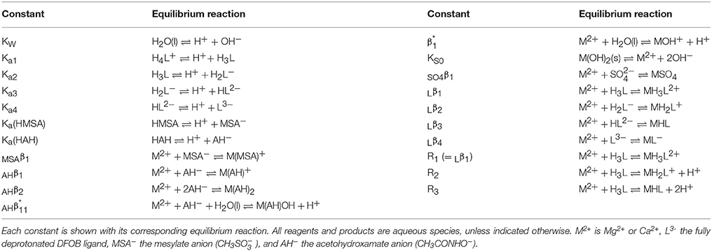
Table 1. Definitions of equilibrium constants used throughout the text.
Results
Stability Constants of Mg−MSA and Ca−MSA Complexes
Desferrioxamine B is a linear molecule with three evenly spaced hydroxamic acid groups and an amine group at one end (Figure 1A). The hydroxamic acid groups deprotonate in the pH range 8.5–9.7, while the amine group is predominantly protonated below pH 10.9 (Christenson and Schijf, 2011). The sequential deprotonation of DFOB can be written as
with acid dissociation constants
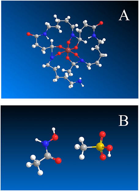
Figure 1. (A) Hexadentate DFOB complex formed by Mg and Ca, with the terminal amine group at the bottom center. (B) Acetohydroxamic acid, CH3CONHOH (left) and methanesulfonic acid, CH3SO2OH (right). Gray, C; white, H; red, O; blue, N; yellow, S; brown, Mg or Ca.
At non-alkaline pH, fully protonated DFOB, H4L+, carries a single positive charge. Solid DFOB therefore requires a counter-ion with a single negative charge to make a neutral compound. A standard pharmaceutical DFOB preparation, marketed under the brand name Desferal®, uses the methanesulfonate anion (MSA−), often called mesylate. Its protonated form is methanesulfonic acid, or HMSA (Figure 1B).
Hernlem et al. (1996) noted that the inevitable presence in DFOB solutions of an equal amount of MSA− could lead to a bias in potentiometric titrations if the latter forms fairly stable complexes with the analyte metal. However, they were unable to determine the pKa of HMSA, which they believed to be 1.92 from the NIST database (Martell et al., 2004) but found to be certainly < 0.9. Christenson and Schijf (2011) pointed out that the NIST database contains a sign error and that the actual value is −1.92 (Covington and Thompson, 1974), congruent with the observation of Hernlem et al. (1996). Because of this extremely low pKa value, metal–MSA complexes do not dissociate within our experimental pH window (~2–11) and their stability constants cannot be directly determined by potentiometric titration. Yet, if stable enough, MSA complexes will effectively increase the concentration of the free metal cation, from which they cannot be distinguished since their formation does not elicit a change in pH, and thereby lower the apparent stability constants of complexes with DFOB or other ligands.
In a study of DFOB complexation with yttrium and the rare earth elements (YREEs), Christenson and Schijf (2011) indirectly estimated the stability of the Lu(MSA)2+ complex by comparing the solubility of Lu(OH)3(s) in the absence and presence of MSA− and found it to be similar to the stability of the structurally related Lu–sulfate complex. They concluded that, with respect to the YREEs, MSA− is an 8–13 orders of magnitude weaker ligand than DFOB and thus of no consequence. Assuming, for lack of evidence to the contrary, that the stabilities of MSA and sulfate complexes are broadly interchangeable, Schijf et al. (2015) drew the same conclusion in a study of DFOB complexation with Cu, Ni, Zn, Cd, and Pb.
The outcome is different if this rule is applied to Mg and Ca. Stability constants, log SO4β1, of the Mg–sulfate and Ca–sulfate complex are 1.01 and 1.03, respectively, at I = 0.7 (Millero and Schreiber, 1982), whereas previous estimates of the stability constant, log Lβ3 of the hexadentate Mg–DFOB and Ca–DFOB complex are about 3–4 (Farkas et al., 1999). In this case, DFOB may be a no more than three orders of magnitude stronger ligand than MSA− (Tables 5, 8). The hydroxide salts of Mg and Ca are poorly characterized and fairly soluble (Martell et al., 2004), hence precipitation cannot be used to determine the stability of their MSA complexes, as for Lu (Christenson and Schijf, 2011). However, the aforementioned effect of MSA complexation on potentiometric titrations works to our advantage if we compare the stability constants of Mg and Ca complexes with a suitable ligand in the absence and presence of MSA−. If the acid dissociation constant of an arbitrary ligand HY and the stability constant of its complex with a divalent metal M are defined as follows (omitting charges for convenience):
then, in the presence of MSA−, the constant Yβ1 will instead be determined as
If we define the stability constant of the complex M(MSA)+ as
(Table 1), it can be shown, by combining Equations (4) and (5), that
The stability constant MSAβ1 can therefore be calculated from Yβ1 and , measured in the absence and presence of MSA−, respectively. If MSAβ1 is small i.e., if [M(MSA)+] ≪ [MSA]T, we can assume that [MSA−] = [MSA]T − [HMSA] − [M(MSA)+] ≈ [MSA]T, since MSA− does not protonate.
Initially, oxalate, −OOC−COO−, and malonate, −OOC−CH2−COO−, were considered for the ligand Y. They form bidentate Mg and Ca complexes with stabilities similar to those of the hexadentate DFOB complexes, so their potentiometric titrations should be affected by MSA− to a comparable degree. Unfortunately, these diprotic ligands may bind metals with only one of their carboxylate groups (cf. Schijf and Byrne, 2001) and the first dissociation constant of oxalic acid lies just outside the experimental pH window (pKa1 ~ 1; Kettler et al., 1998), which complicated interpretation of the titration curves. Our choice ultimately fell on acetohydroxamic acid or HAH, CH3–CO–NHOH (Figure 1B), a monoprotic acid that essentially has the same properties as each of the three hydroxamic acid groups in DFOB.
First, pKa was determined from 9 titrations of HAH alone in 0.7 M NaClO4 at concentrations ranging from 5 to 20 mM (Table 2). Two of these titrations were performed in the presence of 70 mM and one in the presence of 140 mM MSA−, which was added as NaMSA in order to not unduly acidify the experimental solutions. The pKa values measured in these three titrations were not discernibly different from those measured in the other six, showing as expected that the presence of MSA−, in itself, had no effect on the pH of the solution. The 9 titrations together yield an average value of pKa = 9.257 ± 0.008 (Table 5), in beautiful agreement with published measurements of 9.35 in 0.1 M NaNO3 (Anderegg et al., 1963) and 9.27 ± 0.01 in 0.2 M KCl (Farkas et al., 1999). Unlike the large, linear DFOB molecule (Christenson and Schijf, 2011), equilibrium constants for the small HAH molecule should display Debije–Hückel-like behavior and the value of pKa does indeed seem to decrease with increasing ionic strength. Values of are on the order of 100 μM and alternate randomly between proton excess and deficiency. Modeled total HAH concentrations are about 1–4% higher than gravimetric concentrations, with the greatest difference observed at 5 mM HAH (Table 2).
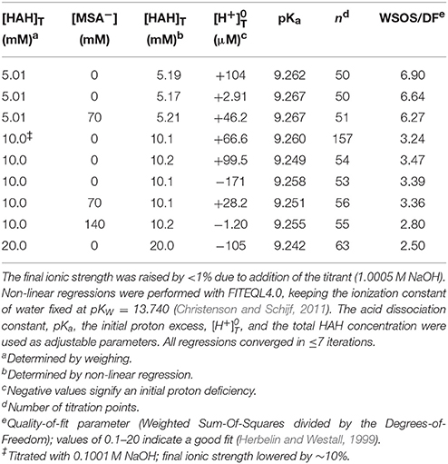
Table 2. Nine titrations (pH 3–11) of acetohydroxamic acid (HAH) in 50 mL of 0.7 M NaClO4 solution, some in the presence of mesylate (MSA−).
Next, Mg and Ca were titrated in the presence of 5 or 10 mM HAH at nominal M:L ratios of 1:2, 1:1, and 2:1. Six Ca and seven Mg titrations were conducted with HAH alone and six more of each in the presence of 140 mM NaMSA (Tables 3, 4), the highest concentration that was shown not to affect the pKa measurements. The stability constants of metal–AH complexes and the initial proton excess, , were used as adjustable parameters in non-linear regressions of the titration curves, whereas the total ligand concentration was fixed at the gravimetric value. For Ca, only the Ca(AH)+ complex was needed to produce good fits (WSOS/DF < 1.2). Values of log AHβ1 were determined to be 2.30 ± 0.03 and 2.25 ± 0.01 in the absence and presence of MSA−, respectively (Table 5), comparing favorably with literature values of 2.4 at I = 0.1 (Anderegg et al., 1963) and 2.45 ± 0.01 at I = 0.2 (Farkas et al., 1999). The value of log MSAβ1, calculated from these averages with Equation (6), is equal to −0.005 (Table 5), but could be as high as 0.2 or as low as –0.4 within the uncertainty of the measurements.
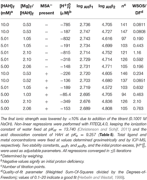
Table 3. Thirteen titrations (pH 3–10) of magnesium in 0.7 M NaClO4 solutions containing 5 or 10 mM acetohydroxamic acid (HAH), some in the presence of 140 mM mesylate (MSA−).
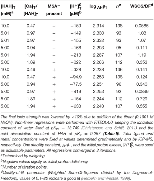
Table 4. Twelve titrations (pH 3–10) of calcium in 0.7 M NaClO4 solutions containing 5 or 10 mM acetohydroxamic acid (HAH), some in the presence of 140 mM mesylate (MSA−).
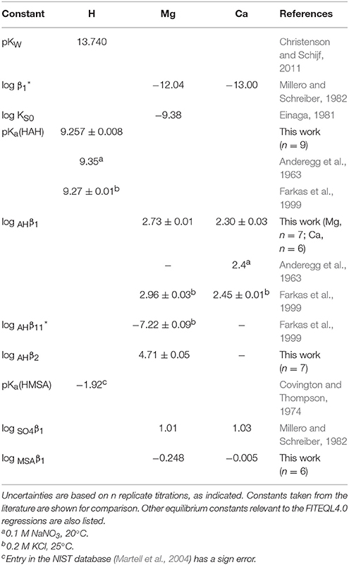
Table 5. Stability constants for AH and MSA complexes of Mg and Ca, derived from potentiometric titrations.
For Mg, inclusion of only the Mg(AH)+ complex produced much poorer fits than for Ca (WSOS/DF ≤ 3.5). Addition of the ternary Mg(AH)OH complex, purportedly observed by Farkas et al. (1999), does not significantly improve the fits, while the corresponding stability constant, log , is similar to that of the MgOH+ complex and two orders of magnitude lower than the value found by these authors and therefore does not constitute independent prove of its formation. Instead, inclusion of a second-order complex, Mg(AH)2, does improve the regressions (WSOS/DF < 2.1) and yields stability constants of the expected absolute and relative magnitude: log AHβ1 = 2.73 ± 0.01 and log AHβ2 = 4.71 ± 0.05 (Table 5). The only literature value for log AHβ1 is 2.96 ± 0.03 at I = 0.2 (Farkas et al., 1999). The second-order complex had not been previously recognized, yet is known to exist for many other divalent metals (Anderegg et al., 1963). Titrations in the presence of MSA− yield log AHβ1 = 2.70 ± 0.02 and log AHβ2 = 4.7 ± 0.1. Average values of log AHβ2 are statistically equal for the two systems, but log AHβ1 values are consistent with log MSAβ1 = −0.248 (Table 5), although it could be as high as 0.03 or as low as −1.1 within the uncertainty of the measurements. The value of ranges from about −200 to −500 μM for all Mg and Ca titrations, indicating a proton deficiency likely caused by lower accuracy of the glass electrode at the very low pH of the metal standards (Section Preparation of Reagents and Standards).
It is clear from the upper-bound values of log MSAβ1 that complexation of Mg and Ca with MSA− is exceedingly weak, specifically quite a lot weaker than their complexation with sulfate, contrary to what was found for Lu (Christenson and Schijf, 2011). It is noteworthy that, like the corresponding sulfate complexes, the Ca(MSA)+ complex appears to be more stable than the Mg(MSA)+ complex, which is not seen for complexes with AH− and DFOB (Section Stability Constants of Mg–DFOB and Ca–DFOB Complexes) and not what one would expect based on the smaller ionic radius of Mg2+. Whereas the MSA complexes were included in the regression models for the DFOB titrations (Section Stability Constants of Mg–DFOB and Ca–DFOB Complexes), compositions of the experimental solutions, calculated with FITEQL4.0, suggest that their contributions to the total Mg and Ca concentrations are ≪1%.
Stability Constants of Mg–DFOB and Ca–DFOB Complexes
Following assessment of the stability of their MSA complexes, titrations of Mg and Ca in the presence of DFOB could be evaluated. Since MSA− is the DFOB counter-ion, these titrations always contained equal concentrations of DFOB and MSA− i.e., substantially less MSA− than was added in the HAH titrations. Since Mg and Ca complexes with DFOB were expected to be at most as stable, and probably less stable, than their complexes with AH− (Tables 5, 8), the potentiometric signal, reflecting the contribution of Mg and Ca complexes to the total DFOB concentration, was maximized by increasing the M:L ratio as much as possible, whereby the upper limit is set by the solubility of hydroxide salts at high pH. However, unlike the divalent transition metals where M:L ratios had to be kept below 0.7:1 (Schijf et al., 2015), Mg(OH)2(s) is fairly soluble and precipitation of Ca(OH)2(s) is of no concern. Consequently, 9 titrations were performed for Mg with 2 mM DFOB and nominal M:L ratios of 1:1, 3:2, and 2:1 (Table 6), and 9 for Ca with 1 or 2 mM DFOB and nominal M:L ratios of 1:1, 3:2, 2:1, 3:1, and 4:1 (Table 7), requiring maximum Mg or Ca concentrations of ~4 mM. For comparison, the concentrations of Mg and Ca in standard seawater (S = 35) are 54 and 10.5 mM. Compositions of the experimental solutions, calculated with FITEQL4.0, suggest that Mg reached at most 22% of saturation in the DFOB titrations and at most 72% in the HAH titrations, with respect to the “active” form of Mg(OH)2(s) that precipitates before aging to crystalline brucite (Gjaldbaek, 1925; Einaga, 1981).
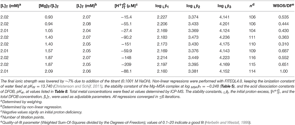
Table 6. Nine titrations (pH 3–10) of magnesium in 0.7 M NaClO4 solutions containing equal amounts of DFOB and MSA−.
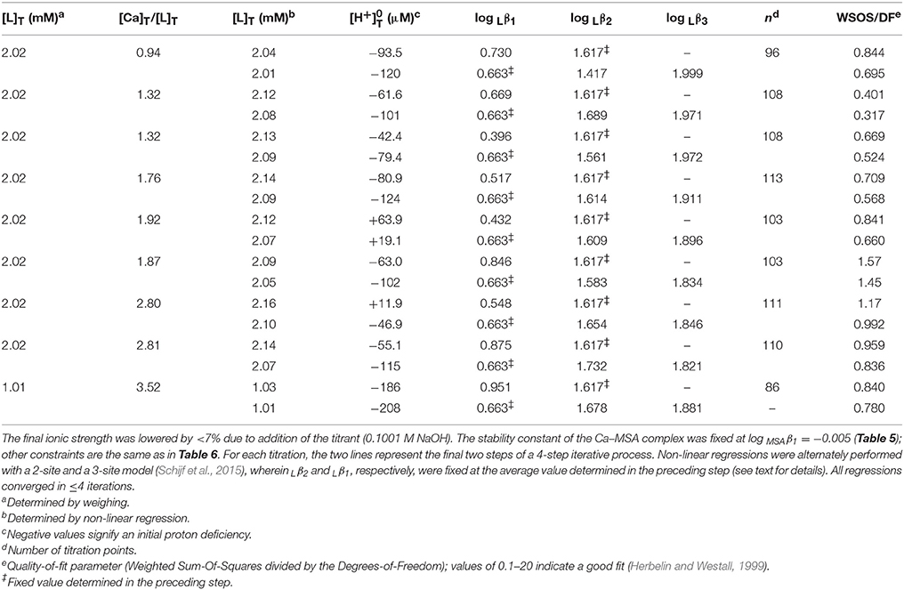
Table 7. Nine titrations (pH 3–10) of calcium in 0.7 M NaClO4 solutions containing equal amounts of DFOB and MSA−.
In non-linear regressions of the Mg and Ca titrations with DFOB, stability constants, log Rj (Table 1), the initial proton excess, , and the total DFOB concentration were used as adjustable parameters. The Mg titrations yield average values of log Lβ1 = 2.19 ± 0.02, log Lβ2 = 3.41 ± 0.04, and log Lβ3 = 4.17 ± 0.04 (Table 8). This confirms that Mg forms a bidentate complex with DFOB, which could not be resolved by Farkas et al. (1999), but lends no support to Mg coordination with the terminal amine (Figure 1A). Fits are of good quality (WSOS/DF ~ 0.3–1.0) and modeled total DFOB concentrations exceed gravimetric concentrations by no more than ~2%. Values of are always negative, ranging up to a proton deficiency of about 200 μM, in agreement with the HAH titrations.
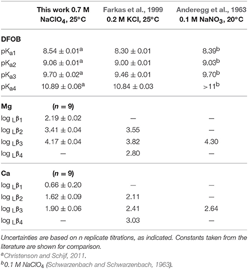
Table 8. Stability constants for DFOB complexes of Mg and Ca, derived from potentiometric titrations.
For Ca, DFOB complexation is so weak (Figure 2) that the 3-site model used for Mg was under-constrained and the three stability constants could not be determined simultaneously. The fits were therefore executed in several steps. In the first step, a 2-site model was used (Schijf et al., 2015), including only log Lβ1 and log Lβ2, for which all regressions converged. In the second step, log Lβ1 was fixed to the average value, 0.73 ± 0.17, obtained in the first step and used with the full 3-site model to obtain values for log Lβ2 and log Lβ3. These two steps were repeated, fixing log Lβ2 obtained from the second step in the third step, and then log Lβ1 obtained from the third step in the fourth and final step. The regressions from step 3 and 4 are shown in Table 7. Average values of log Lβ1 = 0.66 ± 0.20 (from step 3) and of log Lβ2 = 1.62 ± 0.09 and log Lβ3 = 1.90 ± 0.06 (from step 4) are listed in Table 8.
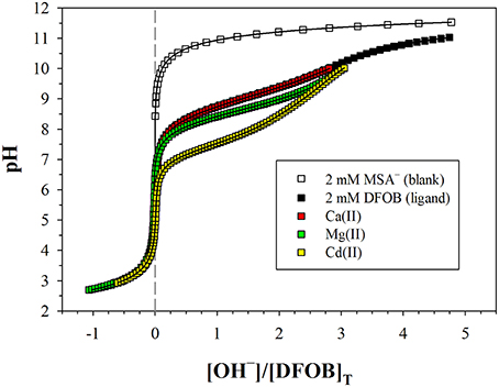
Figure 2. Potentiometric titrations of a DFOB solution and metal+DFOB mixtures in 0.7 M NaClO4, where pH is plotted against moles of base (OH−) added per mole of DFOB. The blank contains 2 mM mesylate (MSA−), which is fully deprotonated over the entire pH range. All other solutions contain 2 mM DFOB mesylate. Symbols are measurements. Solid lines are non-linear regressions performed with FITEQL4.0. The more a metal+DFOB titration deviates from that of DFOB alone, the higher the stability of the metal–DFOB complexes formed. Note that the DFOB and Ca+DFOB titrations are almost indistinguishable. Cadmium (Cd), which forms the weakest hexadentate complex among the divalent transition metals (Schijf et al., 2015), is shown for comparison. The M:L ratio is about 1:1 for Mg and Ca, and about 0.7:1 for Cd.
Subsequent regressions of the titration curves with the unconstrained 3-site model and using 0.66 as the starting value for log Lβ1 did not yield meaningful results, which shows that the lack of convergence is not caused by a poor initial guess for this parameter. Speciation calculations for the experimental solutions, based on the results in Table 8, reveal that insensitivity to the value of log Lβ1 reflects the minute contribution of the corresponding CaH3L2+ complex to the total DFOB concentration. Its absolute contribution was increased by raising the M:L ratio (Table 7), which is however bound by other concerns like hydrolysis. Even at our highest M:L ratio of 4:1, the maximum relative contribution of the bidentate complex is only about 0.7% (at pH 8.7) of the total DFOB concentration. A sensitivity analysis was performed by repeating the final regression step for all 9 titrations with log Lβ1 fixed at values ranging from 2σ below to 2σ above the mean in increments of 0.1 and recording the resulting values of log Lβ2 and log Lβ3. The standard deviations of the values thus obtained are no larger than the errors derived from the 9 independent titrations (Table 8), indicating that the latter are a good estimate of the uncertainty inherent in this iterative regression process. A better estimate of the true errors might be obtained from a simultaneous fit of all titration curves, were it not that such a large dataset with multiple total metal and ligand concentrations surpasses the capability of FITEQL4.0.
The final fits (Table 7) are of good quality (WSOS/DF ~ 0.3–1.5) and modeled total DFOB concentrations exceed gravimetric concentrations by no more than 3–4%. Values of range from a proton deficiency of about 200 μM to an excess of 20 μM, probably reflecting the slightly higher pH of the Ca standards. There is no evidence for Ca coordination with the terminal amine (Figure 1A) and the bidentate Ca–DFOB complex, which again could not be resolved by Farkas et al. (1999), is even less stable than the bidentate Mg–DFOB complex (Table 8). Both our Mg and Ca data yield positive step-wise stability constants for each consecutive hydroxamate bond (Section Calculation of the Side-Reaction Coefficient and Comparison with Published Data).
Discussion
Calculation of the Side-Reaction Coefficient and Comparison with Published Data
Our new DFOB speciations in the presence of Mg and Ca, presented in Table 8, are rather different than those reported by Farkas et al. (1999). Although their potentiometric data appears to be of excellent quality, these authors routinely include in their regression models a stability constant for metal complexes with fully deprotonated DFOB, implying coordination of the metal cation with the DFOB terminal amine. However, while such a complex may exist for some tetravalent cations like Sn4+ (Hernlem et al., 1996) and Hf4+ (Yoshida et al., 2004), it has not been found for other highly charged cations like Th4+ (Whisenhunt et al., 1996) or the trivalent lanthanides (Christenson and Schijf, 2011) and is very unlikely to form with Mg2+ and Ca2+. Schijf et al. (2015) emphasized that adding this extra degree of freedom to the regression model can lead to under-constrained fits and probably explains why Farkas et al. (1999) were unable to resolve values for log Lβ1, whereas the bidentate DFOB complex, analogous to the bidentate AH complex (Table 5), is certainly expected to form as the first of three equivalent steps leading to the stable hexadentate DFOB complex. It also accounts for the fact that values of log Lβ2, log Lβ3, and log Lβ4, reported by Farkas et al. (1999) and shown in Table 8, are either nearly identical or actually become smaller, resulting in thermodynamically anomalous behavior of the step-wise stability constants, log Kj+1 = log Lβj+1 − log Lβj (Schijf et al., 2015). Calculated from our data, these step-wise stability constants are log K2 = 3.41–2.19 = 1.22 and log K3 = 4.17–3.41 = 0.76 for Mg; and log K2 = 1.62–0.66 = 0.96 and log K3 = 1.90–1.62 = 0.28 for Ca (Table 8). We find as expected that (i) they are all of similar magnitude since in each step a bond is formed with a single hydroxamate group; (ii) log K3 < log K2 since the charge of the central cation in each step is shielded by the bond formed in the preceding step; and (iii) the values are lower for Ca2+ being the larger of the two ions. In contrast, Farkas et al. (1999) found log K3 and log K4 equal to 0.27 and −1.02 for Mg, and 0.30 and 0.62 for Ca, respectively. Their step-wise constants show no systematic pattern and furthermore suggest weak binding to the third hydroxamate group, inconsistent with the high values of log Lβ2 (Table 8). Again, this is ostensibly due to regression of the data with an incorrect speciation model, not to poor quality of the data itself.
Wuttig et al. (2013) used the speciations of Farkas et al. (1999), appropriate for 0.2 M KCl, to calculate the SRC of DFOB in seawater, obtaining log αDFB = 6.25. While the authors presented the data on which the calculation is based (Farkas et al., 1999), they provided no additional information, yet αDFB appears to be the ratio of the total ligand and the fully deprotonated free-ligand concentrations, LT/[L3−]. This choice was evidently inspired by the equilibrium constants of Farkas et al. (1999), which are all expressed in terms of L3−. The calculation of Wuttig et al. (2013) is reproduced in detail in the third column of Table 9. Each line represents a DFOB solution species, X, which include L3− and the four protonated forms, as well as the complexes with Mg considered by Farkas et al. (1999), MgH3L2+, MgHL, and MgL−, and similarly for Ca. Each number in the third column represents the ratio [X]/[L3−], where the entry corresponding to X = L3− is of course [L3−]/[L3−] = 1, per definition. The sum of all species equals the total concentration, hence the sum of these ratios equals LT/[L3−] = αDFB (referred to in Table 9 as ∑αL). Column 4 contains our own calculation of this SRC, using data from Christenson and Schijf (2011) and the present work, appropriate to seawater ionic strength. Column 2 specifies how each ratio [X]/[L3−] is derived from the proton concentration and equilibrium constants listed in Table 8.
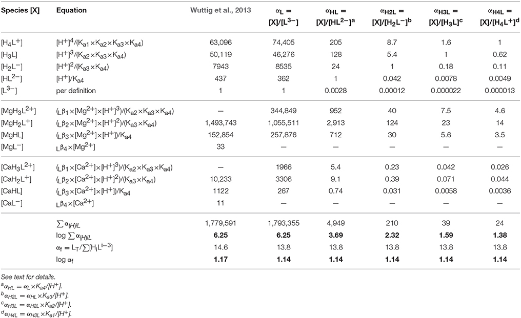
Table 9. Calculation of the side-reaction coefficient of DFOB in seawater, using the data from Table 8.
The outstanding agreement between our SRC and that of Wuttig et al. (2013) should not be surprising, despite the distinct disagreement between our measured Mg–DFOB and Ca–DFOB stability constants and those of Farkas et al. (1999). Remember that this disagreement is not the result of bad titration data, but of an incorrect speciation model used to interpret these data. Our acid dissociation constants and those of Farkas et al. (1999) are very close (Table 8) and while the distributions of Mg–DFOB and Ca–DFOB complexes are different, the total still adds up to LT in each case. Specifically, the sum of the Mg complexes in column 3 and 4 differs by < 1% and while the sum of the Ca complexes differs by more than a factor 2, the latter are only a minor fraction of the total DFOB concentration. Nevertheless, the agreement is somewhat fortuitous for several reasons. First, it seems that Wuttig et al. (2013) used total rather than free concentrations of Mg and Ca, which are about 89% of total concentrations in seawater (Byrne, 2002), primarily as a result of sulfate complexation. Second, Wuttig et al. (2013) expressed pH on the total scale (pHT = −log{[H+]+[ ]}), commonly used for seawater, instead of the free scale (pHf = −log [H+]), where pHT = pHf + 0.13 at S = 35 and T = 25°C (Byrne, 2002). Finally, Wuttig et al. (2013) attempted to extrapolate the stability constants of Farkas et al. (1999) to seawater ionic strength, which is erroneous because chelates do not conform to Debije–Hückel-type behavior (Anderegg et al., 1963) and equilibrium constants for DFOB have been shown to display little or no ionic strength dependence (Christenson and Schijf, 2011). These corrections seem to have canceled each other out to some extent.
A more relevant issue is the interpretation of the constant ∑αL (= αDFB). It says that the ratio [L3−]/LT ≈ 10−6.25 = 5.6 × 10⁻⁷, implying that only a vanishingly small fraction of the total DFOB concentration is available to form complexes, even in the absence of competing trace metals (like Fe3+). Yet it should be kept in mind that there are four other, protonated forms of the ligand and that the choice of L3− to calculate the SRC, albeit a natural one for many polyprotic ligands, is awkward for DFOB. The reason is that, due to a pKa4 of 10.89 (Table 8), L3− is an entirely negligible species in seawater. The top diagrams in Figure 3 show DFOB speciations calculated for trace-metal-free seawater, excluding or including the effect of Mg and Ca. When complexes with Mg and Ca are ignored, >99% of DFOB is made up of the three most protonated species and the species L3− contributes a mere 0.00077%. Moreover, trace metals form the strongest and most abundant complexes with the protonated species, HL2− and H2L−, and less abundant ones with H3L (Schijf et al., 2015). Complexes with L3−, which would involve full coordination of the metal center with the DFOB terminal amine (Figure 1B), have not been definitively proven to exist, except for one or two tetravalent metal cations. In reality, as shown in the right-hand diagram, ~92% of DFOB is complexed with Mg (and < 1% with Ca). Within the ~7% of the total DFOB concentration not complexed with Mg and Ca, the distribution of species is identical to that in the left-hand diagram. In other words, DFOB complexation with Mg and Ca further reduces the contribution of the species L3− by a factor 100/7 ≈ 14. Hudson et al. (1992) used the kinetics of Fe–DFOB complexation to estimate the rate of water loss from the first hydration sphere of Fe(III), but calculated that only about 28% of DFOB in seawater is bound to Mg. The much larger fraction of Mg-bound DFOB established here intimates higher rates of water loss, which has repercussions for the kinetics of Fe complexation with other strong organic ligands in seawater, yet a detailed discussion of this issue is outside the scope of our paper.
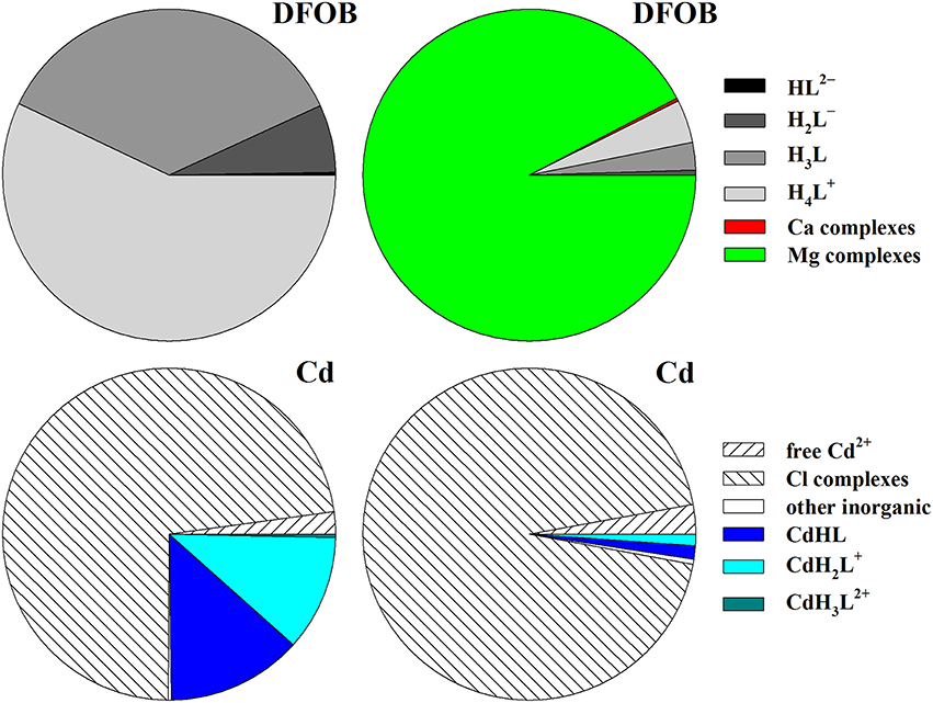
Figure 3. Speciation in seawater (S = 35, T = 25°C) of 10 pM DFOB (top) and of 1 pM Cd (bottom), calculated with MINEQL and shown as fractions of the total concentration. For Cd, the free concentration of the species HL2− was arbitrarily fixed at a value where DFOB complexes comprise about 25% of the total metal concentration. Diagrams on the left do not account for DFOB complexation with Mg and Ca. In diagrams on the right the calculations are repeated with Mg–DFOB and Ca–DFOB complexes explicitly included. Wedges with the word “complexes” are the sum of multiple species. The wedge “other inorganic” refers to Cd complexes with sulfate and carbonate. Species contributing < 0.3% cannot be resolved in the graph.
The remaining columns of Table 9 contain calculations of SRCs corresponding to each of the four protonated DFOB species. It should be noted that the logarithmic values of these constants decrease rapidly with increasing protonation from 6.25 to 1.38, reflecting the contribution of each species to the total DFOB concentration in seawater (Figure 3). In the next section we more thoroughly discuss the (dis)advantages of different SRCs for calculating metal speciation in the presence of DFOB and other strong organic ligands, and present a more convenient definition of the SRC of DFOB in trace-metal-free seawater.
Implications for Model Calculations of Metal and DFOB Speciation in Seawater
The concept of SRCs was formalized and their proper use demonstrated by Ringbom and Still (1972). In general, they are a means of correcting free ligand (or metal) concentrations for complexation with cations in the background electrolyte and with competing metals (or ligands), without having to explicitly account for each complex in a speciation model. Their main benefit lies in the calculation of “conditional” stability constants and most of us are familiar with that approach in systems where a metal forms single 1:1 or higher-order complexes with one or more ligands, and vice versa. The situation becomes more complicated for large polyprotic, polydentate ligands, which can form more than one type of 1:1 complex with a single metal. The SRC ∑αL (= αDFB) calculated by Wuttig et al. (2013), can be used to correct metal speciations in seawater in the presence of DFOB for DFOB complexation with Mg and Ca. With a speciation code like MINEQL (Westall et al., 1986), the easiest way is to fix the free concentration of L3− at the value ∑αL × LT and to calculate the metal speciation with elimination of all other DFOB complexes (except for protonation steps), provided all stability constants are expressed in terms of L3− and appropriate to seawater ionic strength. Alternatively, if stability constants are expressed in terms of HL2−, its free concentration has to be fixed at the value ∑αHL × LT (Table 9), and so forth for any of the protonated DFOB species. However, these SRCs cannot be used in the sense intended by Ringbom and Still (1972). It is possible to create “conditional” metal–DFOB stability constants by subtracting log ∑α(H)iL from thermodynamic stability constants expressed in terms of HiL, but these can only be employed in MINEQL either if log ∑α(H)iL is also subtracted from the acid dissociation constants, or if the protonation steps are eliminated altogether and the free concentration of HiL is fixed at the total concentration, LT. Both yield the correct metal speciation, but the distribution of uncomplexed DFOB among its protonated species will be greatly skewed.
Our primary purpose is to determine an SRC allowing calculation of metal–DFOB stability constants that can be meaningfully compared with the results of ACSV-CLE analyses, which produce conditional stability constants of metal complexes with unknown organic ligands in seawater (Pižeta et al., 2015). In the typical representation of metal–DFOB stability (Table 8), each constant Lβj is expressed in terms of the protonated DFOB species that forms the corresponding complex (Anderegg et al., 1963; Hernlem et al., 1996; Schijf et al., 2015) and would therefore have to be corrected by subtracting a different SRC. However, it is possible to define one single SRC that can correct all metal–DFOB stability constants, regardless of how they are expressed. This is the constant αf = LT/∑[HiL], where the denominator is the sum concentration of all DFOB species that are not complexed with Mg or Ca. The underlying principle is that speciation models do not include trace metal complexation by displacement of Mg or Ca from DFOB complexes. In other words, the constant αf represents the fraction of DFOB that is available for metal complexation in seawater. This correction is valid as long as the speciation of DFOB is not significantly altered by the presence of the metal. The value of log αf, shown in Table 9, is the same for each manner of expressing the stability constants. This means that any log Lβj can be converted to a conditional constant for seawater by subtracting 1.14. The value of log αf calculated for the speciation of Farkas et al. (1999) is slightly higher, primarily due to a somewhat greater contribution from the Ca–DFOB complexes. It should be mentioned here that the constant αf, like the constants ∑α(H)iL, is not only dependent on the composition of seawater, which does not vary much throughout the ocean, but also on pH. Values of log ∑αH, log ∑αHL, and log αf, calculated as in Table 9 over a range of pH relevant to seawater, are shown in Figure 4. Note that the pH dependence of the SRC defined by Wuttig et al. (2013) is opposite to and much larger than that of log αf.
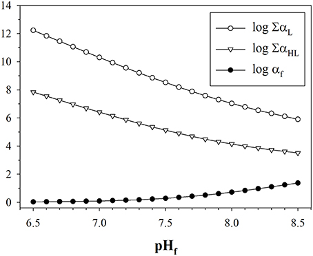
Figure 4. Dependence of the side-reaction coefficients log ∑αL, log ∑αHL, and log αf (Table 9) on seawater pH (free scale). The pH dependence of Mg and Ca free-ion concentrations, which mostly reflects their complexation with sulfate, is negligible and was ignored.
A typical example of a speciation calculation is shown in the bottom diagrams of Figure 3. On the left is the speciation of dissolved Cd (1 pM), which has the lowest affinity for DFOB among the divalent transition metals (Schijf et al., 2015), where DFOB complexation with Mg and Ca is deliberately excluded. The total DFOB concentration (1.33 × 10⁻⁴ M) was arbitrarily chosen so that the contribution of DFOB complexes to the total Cd concentration is almost exactly 25%, the remaining 75% being dominated by Cl complexes, with only ~2% free Cd2+. This concentration is clearly not realistic and only used here to illustrate the effect of DFOB complexation with the major seawater cations. The speciation was calculated with MINEQL, expressing all DFOB stability constants in terms of HL2−. On the right is the speciation calculated for the same total Cd and DFOB concentrations, but with Mg–DFOB and Ca–DFOB complexes explicitly accounted for. It can be seen that the fraction of the total Cd concentration complexed with DFOB is lowered by a factor 101.14 = 13.8 (cf. Section Calculation of the Side-Reaction Coefficient and Comparison with Published Data). The contributions of all chloride complexes and free Cd2+ are proportionally increased. The presence of Mg and Ca thus effectively lowers the amount of DFOB available for complexation by about an order of magnitude. The same result is obtained if all Mg–DFOB and Ca–DFOB complexes are removed from the calculation and log αf = 1.14 is subtracted from the Cd–DFOB stability constants (but not the acid dissociation constants) and this is true regardless of what DFOB species is chosen as the “component” in the MINEQL model (Morel and Morgan, 1972).
Schijf et al. (2015) measured stability constants for DFOB complexes with Ni, Cu, Zn, Cd, and Pb at seawater ionic strength and compared these with conditional constants for complexes with unknown organic ligands in seawater, acquired by voltammetric techniques. Based on the speciation of Farkas et al. (1999), the authors estimated that a proper comparison would require log αf = 1.1 to be subtracted from the measured stability constants, log Lβj, which did not alter their conclusion that natural ligands could be siderophore-like for Cu, Zn, and Pb, but not for Ni and Cd. Our new DFOB speciation shows that their estimate of log αf was satisfactory.
This discussion highlights some of the theoretical challenges that attend the interpretation of voltammetric data and the calculation of SRCs for unknown ligands. Although measurements indicate that a metal may interact with more than one class of ligand (L1, L2), it is normally assumed that only single 1:1 complexes occur, presumably involving the fully deprotonated forms (e.g., Coale and Bruland, 1988). However, all natural organic ligands described so far, including those specific to metals other than Fe (Springer and Butler, 2016), are large polyprotic, polydentate molecules that are likely capable of forming more than one 1:1 complex with the metal, depending on conditions. Our investigations of DFOB complexation have revealed that some metals form the most stable complex with the single-protonated species, some with the double-protonated species, yet none with the fully deprotonated species. In addition, at seawater pH, some metals, like Cd (Figure 3) and Zn, may form multiple DFOB complexes in approximately equal amounts. The relative contributions of multiple complexes formed with a single ligand, which ACSV-CLE theory gathers into one cumulative conditional stability constant, are moreover pH dependent (Figure 4). These caveats are particularly salient because voltammetric analyses are rarely executed at ambient pH (Moffett and Dupont, 2007). Until the identities of natural organic ligands and their individual properties are more completely understood, the interpretation of measured conditional stability constants for their complexes with bio-essential metals and the correct definition of their (pH-dependent) SRCs in seawater remains fraught with ambiguity and must be undertaken with sensible caution.
Author Contributions
JS designed the experiments, performed most of the titrations, conducted all non-linear regressions and speciation calculations, and wrote the manuscript. SMB performed some of the titrations and calculated the side-reaction coefficients.
Funding
The REU project of SMB was funded by NSF (OCE-1262374) and administered by the Maryland Sea Grant Program. Financial support for publication in open-access journals is provided by the University of Maryland.
Conflict of Interest Statement
The authors declare that the research was conducted in the absence of any commercial or financial relationships that could be construed as a potential conflict of interest.
Acknowledgments
Alison Zoll rendered the molecular structure in Figure 1A with ChemDraw v.12.0. Our manuscript was significantly improved by the kind comments of reviewers David Turner and Robert Hudson. CBL statistician Dr. Slava Lyubchich gave expert advice on the error analysis of iterative non-linear regressions. We are grateful to the editors of this special volume of Frontiers in Marine Science for allowing us to present our work. This is UMCES contribution #5187.
Supplementary Material
The Supplementary Material for this article can be found online at: http://journal.frontiersin.org/article/10.3389/fmars.2016.00117
References
Anderegg, G., l'Eplattenier, F., and Schwarzenbach, G. (1963). Hydroxamatkomplexe II. Die anwendung der pH-methode. Helv. Chim. Acta 46, 1400–1408. doi: 10.1002/hlca.19630460435
Baars, O., Abouchami, W., Galer, S. J. G., Boye, M., and Croot, P. L. (2014). Dissolved cadmium in the Southern Ocean: distribution, speciation, and relation to phosphate. Limnol. Oceanogr. 59, 385–399. doi: 10.4319/lo.2014.59.2.0385
Baars, O., and Croot, P. L. (2015). Dissolved cobalt speciation and reactivity in the eastern tropical North Atlantic. Mar. Chem. 173, 310–319. doi: 10.1016/j.marchem.2014.10.006
Boiteau, R. M., Fitzsimmons, J. N., Repeta, D. J., and Boyle, E. A. (2013). Detection of iron ligands in seawater and marine cyanobacteria cultures by high-performance liquid chromatography-inductively coupled plassma-mass spectrometry. Anal. Chem. 85, 4357–4362. doi: 10.1021/ac3034568
Bruland, K. W. (1992). Complexation of cadmium by natural organic ligands in the central North Pacific. Limnol. Oceanogr. 37, 1008–1017.
Bundy, R. M., Abdulla, H. A. N., Hatcher, P. G., Biller, D. V., Buck, K. N., and Barbeau, K. A. (2015). Iron-binding ligand and humic substances in the San Francisco Bay estuary and estuarine-influenced shelf regions of coastal California. Mar. Chem. 173, 183–194. doi: 10.1016/j.marchem.2014.11.005
Byrne, R. H. (2002). “Speciation in seawater,” in Chemical Speciation in the Environment, eds A. M. Ure and C. M. Davidson (Oxford, UK: Blackwell Science), 322–357.
Capodaglio, G., Turetta, C., Toscano, G., Gambarom, A., Scarponi, G., and Cescon, P. (1998). Cadmium, lead and copper complexation in Antarctic coastal seawater. Evolution during the austral summer. Intern. J. Environ. Anal. Chem. 71, 195–226.
Christenson, E. A., and Schijf, J. (2011). Stability of YREE complexes with the trihydroxamate siderophore desferrioxamine B at seawater ionic strength. Geochim. Cosmochim. Acta 75, 7047–7062. doi: 10.1016/j.gca.2011.09.022
Coale, K. H., and Bruland, K. W. (1988). Copper complexation in the Northeast Pacific. Limnol. Oceanogr. 33, 1084–1101.
Covington, A. K., and Thompson, R. (1974). Ionization of moderately strong acids in aqueous solution. Part III. Methane-, ethane-, and propanesulfonic acids at 25°C. J. Solution Chem. 3, 603–617.
Einaga, H. (1981). The hydrolytic precipitation reaction of Mg(II) from aqueous NaNO3 solution. J. Inorg. Nucl. Chem. 43, 229–233.
Farkas, E., Enyedy, É., and Csóka, H. (1999). A comparison between the chelating properties of some dihydroxamic acids, desferrioxamine B and acetohydroxamic acid. Polyhedron 18, 2391–2398.
Gjaldbaek, J. K. (1925). Untersuchungen über die löslichkeit des magnesiumhydroxyds. I. Von der Existenz verschiedener modifikationen von magnesiumhydroxyd. Zeitschr. Anorg. Allgem. Chem. 144, 145–168.
Herbelin, A. L., and Westall, J. C. (1999). FITEQL. A Computer Program for Determination of Chemical Equilibrium Constants from Experimental Data. Version 4.0. Report 99-01, Department of Chemistry, Oregon State University, Corvallis, OR.
Hernlem, B. J., Vane, L. M., and Sayles, G. D. (1996). Stability constants for complexes of the siderophore desferrioxamine B with selected heavy metal cations. Inorg. Chim. Acta 244, 179–184.
Hudson, R. J. M., Covault, D. T., and Morel, F. M. M. (1992). Investigations of iron coordination and redox reactions in seawater using 59Fe radiometry and ion-pair solvent extraction of amphiphilic iron complexes. Mar. Chem. 38, 209–235.
Jacquot, J. E., Kondo, Y., Knapp, A. N., and Moffett, J. W. (2013). The speciation of copper across active gradients in nitrogen-cycle processes in the eastern tropical South Pacific. Limnol. Oceanogr. 58, 1387–1394. doi: 10.4319/lo.2013.58.4.1387
Jakuba, R. W., Saito, M. A., Moffett, J. W., and Xu, Y. (2012). Dissolved zinc in the subarctic North Pacific and Bering Sea: its distribution, speciation, and importance to primary producers. Global Biogeochem. Cycle 26:GB2015. doi: 10.1029/2010gb004004
Janz, G. J., Oliver, B. G., Lakshminarayanan, G. R., and Mayer, G. E. (1970). Electrical conductance, diffusion, viscosity, and density of sodium nitrate, sodium perchlorate, and sodium thiocyanate in concentrated aqueous solutions. J. Phys. Chem. 74, 1285–1289.
Kem, M. P., Zane, H. K., Springer, S. D., Gauglitz, J. M., and Butler, A. (2014). Amphiphilic siderophore production by oil-associating microbes. Metallomics 6, 1150–1155. doi: 10.1039/c4mt00047a
Kettler, R. M., Wesolowski, D. J., and Palmer, D. A. (1998). Dissociation constants of oxalic acid in aqueous sodium chloride and sodium trifluoromethanesulfonate media to 175°C. J. Chem. Eng. Data 43, 337–350.
Kruft, B. I., Harrington, J. M., Duckworth, O. W., and Jarzęcki, A. A. (2013). Quantum mechanical investigation of aqueous desferrioxamine B metal complexes: Trends in structure, binding, and infrared spectroscopy. J. Inorg. Biochem. 129, 150–161. doi: 10.1016/j.jinorgbio.2013.08.008
Martell, A. E., Smith, R. M., and Motekaitis, R. J. (2004). NIST Critically Selected Stability Constants of Metal Complexes. NIST Standard Reference Database 46 Version 8.0. Texas A&M University.
Martin, J. D., Ito, Y., Homann, V. V., Haygood, M. G., and Butler, A. (2006). Structure and membrane affinity of new amphiphilic siderophores produced by Ochrobactrum sp. SP18. J. Biol. Inorg. Chem. 11, 633–641. doi: 10.1007/s00775-006-0112-y
Martinez, J. S., Zhang, G. P., Holt, P. D., Jung, H.-T., Carrano, C. J., Haygood, M. G., et al. (2000). Self-assembling amphiphilic siderophores from marine bacteria. Science 287, 1245–1247. doi: 10.1126/science.287.5456.1245
Mawji, E., Gledhill, M., Milton, J. A., Tarran, G. A., Ussher, S., Thompson, A., et al. (2008). Hydroxamate siderophores: occurrence and importance in the Atlantic Ocean. Environ. Sci. Technol. 42, 8675–8680. doi: 10.1021/es801884r
McCormack, P., Worsfold, P. J., and Gledhill, M. (2003). Separation and detection of siderophores produced by marine bacterioplankton using high-performance liquid chromatography with electrospray ionization mass spectrometry. Anal. Chem. 75, 2647–2652. doi: 10.1021/ac0340105
McKnight, D. M., and Morel, F. M. M. (1980). Copper complexation by siderophores from filamentous blue-green algae. Limnol. Oceanogr. 25, 62–71.
Millero, F. J., and Schreiber, D. R. (1982). Use of the ion pairing model to estimate activity coefficients of the ionic components of natural waters. Am. J. Sci. 282, 1508–1540.
Moffett, J. W., and Dupont, C. (2007). Cu complexation by organic ligands in the sub-arctic NW Pacific and Bering Sea. Deep-Sea Res. I 54, 586–595. doi: 10.1016/j.dsr.2006.12.013
Morel, F., and Morgan, J. (1972). A numerical method for computing equilibria in aqueous chemical systems. Environ. Sci. Technol. 6, 58–67.
Neilands, J. B., and Leong, S. A. (1986). Siderophores in relation to plant growth and disease. Ann. Rev. Plant Physiol. 37, 187–208.
Pižeta, I., Sander, S. G., Hudson, R. J. M., Omanović, D., Baars, O., Barbeau, K. A., et al. (2015). Interpretation of complexometric titration data: An intercomparison of methods for estimating models of trace metal complexation by natural organic ligands. Mar. Chem. 173, 3–24. doi: 10.1016/j.marchem.2015.03.006
Ringbom, A., and Still, E. (1972). The calculation and use of a coefficients. Anal. Chim. Acta 59, 143–146.
Ross, A. R. S., Ikonomou, M. G., and Orians, K. J. (2003). Characterization of copper-complexing ligands in seawater using immobilized copper(II)-ion affinity chromatography and electrospray ionization mass spectrometry. Mar. Chem. 83, 47–58. doi: 10.1016/S0304-4203(03)00095-1
Rue, E. L., and Bruland, K. W. (1995). Complexation of iron(III) by natural organic ligands in the Central North Pacific as determined by a new competitive ligand equilibration/adsorptive cathodic stripping voltammetric method. Mar. Chem. 50, 117–138.
Schijf, J., and Byrne, R. H. (2001). Stability constants for mono- and dioxalato-complexes of Y and the REE, potentially important species in groundwaters and surface freshwaters. Geochim. Cosmochim. Acta 65, 1037–1046. doi: 10.1016/S0016-7037(00)00591-3
Schijf, J., Christenson, E. A., and Potter, K. J. (2015). Different binding modes of Cu and Pb vs. Cd, Ni, and Zn with the trihydroxamate siderophore desferrioxamine B at seawater ionic strength. Mar. Chem. 173, 40–51. doi: 10.1016/j.marchem.2015.02.014
Schwarzenbach, G., and Schwarzenbach, K. (1963). Hydroxamatkomplexe I. die stabilität der eisen(III)-komplexe einfacher hydroxamsäuren und des ferrioxamins B. Helv. Chim. Acta 46, 1390–1400.
Springer, S. D., and Butler, A. (2016). Microbial ligand coordination: consideration of biological significance. Coord. Chem. Rev. 306, 628–635. doi: 10.1016/j.ccr.2015.03.013
Town, R. M., and Filella, M. (2000). Dispelling the myths: is the existence of L1 and L2 ligands necessary to explain metal ion speciation in natural waters? Limnol. Oceanogr. 45, 1341–1357. doi: 10.4319/lo.2000.45.6.1341
Trick, C. G. (1989). Hydroxamate-siderophore production and utilization by marine eubacteria. Curr. Microbiol. 18, 375–378.
van den Berg, C. M. G., and Nimmo, M. (1987). Determination of interactions of nickel with dissolved organic material in seawater using cathodic stripping voltammetry. Sci. Total Environ. 60, 185–195.
Vraspir, J. M., and Butler, A. (2009). Chemistry of marine ligands and siderophores. Ann. Rev. Mar. Sci. 1, 43–63. doi: 10.1146/annurev.marine.010908.163712
Waska, H., Koschinsky, A., Ruiz Chancho, M. J., and Dittmar, T. (2015). Investigating the potential of solid-phase extraction and Fourier-transform ion cyclotron resonance mass spectrometry (FT-ICR-MS) for the isolation and identification of dissolved metal-organic complexes from natural waters. Mar. Chem. 173, 78–92. doi: 10.1016/j.marchem.2014.10.001
Westall, J. C., Zachary, J. L., and Morel, F. M. M. (1986). MINEQL. A Computer Program for the Calculation of the Chemical Equilibrium Composition of Aqueous Systems. Version 1. Report 86-01. Department of Chemistry, Oregon State University, Corvallis, OR.
Whisenhunt, D. W. Jr., Neu, M. P., Hou, Z., Xu, J., Hoffman, D. C., and Raymond, K. N. (1996). Specific sequestering agents for the actinides. 29. Stability of the thorium(IV) complexes of desferrioxamine B (DFO) and three octadentate catecholate or hydroxypyridinonate DFO derivatives: DFOMTA, DFOCAMC, and DFO-1,2-HOPO. Comparative stability of the plutonium(IV) DFOMTA complex. Inorg. Chem. 35, 4128–4136.
Whitby, H., and van den Berg, C. M. G. (2015). Evidence for copper-binding humic substances in seawater. Mar. Chem. 173, 282–290. doi: 10.1016/j.marchem.2014.09.011
Wuttig, K., Heller, M. I., and Croot, P. L. (2013). Reactivity of inorganic Mn and Mn desferrioxamine B with O2, , and H2O2 in seawater. Environ. Sci. Technol. 47, 10257–10265. doi: 10.1021/es4016603
Yoshida, T., Ozaki, T., Ohnuki, T., and Francis, A. J. (2004). Interactions of trivalent and tetravalent heavy metal-siderophore complexes with Pseudomonas fluorescens. Radiochim. Acta 92, 749–753. doi: 10.1524/ract.92.9.749.55003
Zane, H. K., Naka, H., Rosconi, F., Sandy, M., Haygood, M. G., and Butler, A. (2014). Biosynthesis of amphi-enterobactin siderophores by Vibrio harveyi BAA-1116: Identification of a bifunctional nonribosomal peptide synthetase condensation domain. J. Am. Chem. Soc. 136, 5615–5618. doi: 10.1021/ja5019942
Keywords: desferrioxamine B, siderophore, potentiometric titration, stability constant, side-reaction coefficient, seawater, magnesium, calcium
Citation: Schijf J and Burns SM (2016) Determination of the Side-Reaction Coefficient of Desferrioxamine B in Trace-Metal-Free Seawater. Front. Mar. Sci. 3:117. doi: 10.3389/fmars.2016.00117
Received: 31 March 2016; Accepted: 20 June 2016;
Published: 13 July 2016.
Edited by:
Sylvia Gertrud Sander, University of Otago, New ZealandReviewed by:
Robert J. M. Hudson, University of Illinois at Urbana-Champaign, USADavid Turner, University of Gothenburg, Sweden
Copyright © 2016 Schijf and Burns. This is an open-access article distributed under the terms of the Creative Commons Attribution License (CC BY). The use, distribution or reproduction in other forums is permitted, provided the original author(s) or licensor are credited and that the original publication in this journal is cited, in accordance with accepted academic practice. No use, distribution or reproduction is permitted which does not comply with these terms.
*Correspondence: Johan Schijf, c2NoaWpmQGNibC51bWNlcy5lZHU=