 Annalisa Di Cicco
 Michela Sammartino
 Salvatore Marullo
 Rosalia Santoleri
- 1Institute of Atmospheric Sciences and Climate, National Research Council (CNR), Rome, Italy
- 2National Agency for New Technologies, Energy and Sustainable Economic Development, Frascati, Italy
Regional relationships to estimate the main Phytoplankton Functional Types (PFTs) and Size Classes (PSCs) from satellite data are presented. Following the abundance-based approach and selecting the Total Chlorophyll a (TChla) as descriptor of the trophic status of the environment, empirical relations between the TChla concentration and seven accessory pigments, marker for the main algal groups, have been developed for the Mediterranean Sea. Using only in-situ data acquired in this basin, firstly a previous regional diagnostic pigment analysis has been conducted to evaluate the specific pigment ratios featuring the phytoplankton assemblage that occurs in the Mediterranean Sea. Secondly, the new regional PFT and PSC algorithms have been calibrated and validated on the in-situ dataset. The statistical analysis showed a very good predictive power for all the new regional models. A quantitative comparison with global abundance-based models applied to our validation dataset showed that the regionalization improves the uncertainty and the spread of about one order of magnitude for all the classes (e.g., in the nano class, where the mean bias error improves from −0.056 to 0.001 mg m−3). These results highlighted that a regionalization for the PSC and PFT estimates are required, to take into account the peculiar bio-optical properties of the Mediterranean Sea. Finally, the new regional equations have been applied to the Mediterranean TChla satellite (1998–2015) time series to estimate annual and monthly PFT and PSC climatology. The analysis of the climatological maps, relative to the phytoplankton assemblage distribution patterns, reveals that all the three size classes reach their maxima in the higher nutrient areas, with absolute values >3 mg m−3 of TChla for micro-, and about 1.6 and 0.4 mg m−3 for nano- and pico-phytoplankton, respectively. Moreover, the nano component shows intermediate percentage values in the whole basin, ranging from 30 to 40% of the TChla in the western basin, up to 45% in the more productive areas. In terms of chlorophyll concentration, in the coastal areas we find the predominance of the Diatoms and Haptophytes, while in the ultra-oligotrophic waters Prokaryotes predominates on the other groups, constituting the principal component of the pico-phytoplankton.
Introduction
Phytoplankton have a key role in the biogeochemistry of the Earth, with a predominant position in several ecological processes as climate regulation, food webs, fossil fuel formation, and correlated economic human activities (Falkowski et al., 2003). The biogeochemical functions performed by the phytoplankton assemblage are closely linked to its composition. Key groups of organisms with their specific biogeochemical metabolism mediate the elemental fluxes in the biosphere (Falkowski et al., 2003; Le Quéré et al., 2005). The composition and succession of various phytoplankton taxa in the community are also a mirror of the ecological status of the marine environment (Devlin et al., 2007). Within this context, in the recent years the scientific interest in the comprehension of the phytoplankton assemblage structure is surging. The methods for the identification of these organisms have strongly evolved, moving from single cell counting and taxonomic identification based on the traditional microscopic techniques to most recent approach based on remote sensing investigation (IOCCG, 2014).
Proper identification of Linnaean taxonomic species that compose a natural phytoplankton assemblage requires the use of multiple combined techniques. By using the classical optical microscopy only, which remains one of the best approaches for the identification of the largest phytoplankton cells, it has been ignored for years the smallest fraction of the phytoplankton, instead detectable through specific techniques such as flow-cytometry, chemotaxonomy, epifluorescence microscopy, size-fractionation, and determination of chlorophyll a content with High Performance Liquid Chromatography, HPLC (Siokou-Frangou et al., 2010). A species-specific identification also requires great time demanding and needs of deep experience in the taxonomy knowledge (Reynolds, 2006). Nowadays, the systematic classification of phytoplankton at the level of phyla and of certain classes is well-established, with the agreement of microscopists and biochemicals (Reynolds, 2006). For several years, one of the most useful techniques for the algal classification at these taxonomic levels has been the HPLC. The liquid chromatography allows the separation, with resulting identification and quantification, of the main algal pigments, some of them considered markers for specific phytoplankton groups (see Table 1). The number of phytoplankton species is by far smaller than the terrestrial plants, but with a greater phylogenetic diversity, strictly related with the principal ecological functions (Falkowski and Raven, 1997; Falkowski et al., 2003). Phylogenetic studies on the oxygenic phytoplankton evolution suggested three main recognizable lineages. The first, in the prokaryotic empire, consists of all the Cyanobacteria. The other two, within the eukaryotic algae, are divided in “green lineage,” characterized by chlorophyll b as secondary pigment and by a small quantity of several carotenoids (Phyla Chlorophyta and Euglenophyta) and in “red-lineage” including Rhodophyta, pigmented with phycobiliproteins and a number of other algal groups characterized by chlorophyll c and a wide variety of carotenoids. These groups involve Cryptophyta, Heterokontophyta, Haptophyta, and probably those Dinophyta pigmented with peridinin (Delwiche, 1999; Falkowski et al., 2003; Reynolds, 2006).
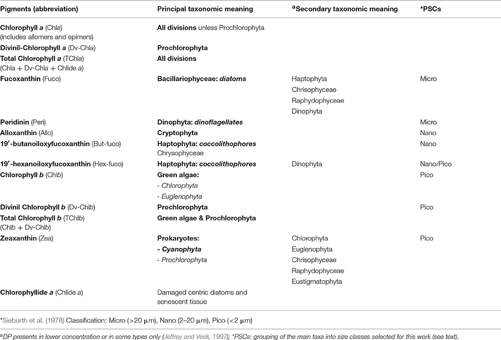
Table 1. Diagnostic Pigments (DP) and their taxonomic meaning in microalgal divisions or classes (Jeffrey and Vesk, 1997; Prezelin et al., 2000; Vidussi et al., 2001; Wright and Jeffrey, 2006; Ras et al., 2008; Brunet and Mangoni, 2010).
In order to better understand the ecological systems and monitor the ecological status of marine environment, the main target is to identify the structures and processes that can explain ecosystem dynamics, linking descriptors of state to descriptors of change. Recent trends in the comprehension of the community structure and functioning are aimed to the research of those “functional traits” species-independent able to act as non-taxonomic “descriptors of community.” Two of the most relevant taxonomic-free descriptors are the body size class and the functional group (Basset et al., 2004; Mouillot et al., 2006).
The definition of “functional group” is open to different interpretations, clustering phytoplankton on the base of various ecological roles and specialized requirements. This term groups species with similar “morphological and physiological traits and ecologies” (Reynolds et al., 2002): a functional group is composed by different species that, starting from the same resource or ecological component, perform a common ecological function (Blondel, 2003). On the basis of their biogeochemical metabolism or, farther, on the “resource” shared by the organisms, main taxonomic phytoplankton groups can be assembled in four specific “functional groups” (Blondel, 2003; Falkowski et al., 2003; Litchman et al., 2007; IOCCG, 2014): nitrogen fixers (this ability is unique to the Prokaryotes), calcifiers (including the taxonomical class of Haptophyceae, generally known as coccolithophores), silicifers (represented by the class of Bacillariophyceae, tipically known as diatoms, followed by some chrysophytes, silicoflagellates, and xanthophytes, which are not very widespread in the Mediterranean Sea), and Dimethylsulfoniopropionate (DMSP) producers (referred to some marine phytoplankton organisms belonging primarily to the group of Dinoflagellates, followed by Haptophytes).
The other important “taxonomic-free” descriptor is the “size.” A great number of single organism and community characteristics depend, in a known manner, on individual dimension. The “metabolic theory” of Brown et al. (2004), closely links the performance of “individuals” in terms of metabolism and energy transfer efficiency to the ecology of “population, community, and ecosystems.” There is a flow of energy and matter between the various ecological systems at different hierarchical scales, depending on environmental and individual characteristics that regulate the metabolism of the single organism and consequently, the features of each hierarchical level. According to this theory, body size, together with temperature and stoichiometry, is one of three key factors that affect individual metabolism and, consequently, the community ecology.
Although, also size measurements may be affected by uncertainties, especially at ecological “individual” level, morphometric, or “body size” descriptors offer however important advantages with respect to the taxonomic ones: cell size is simpler to measure in quantitative and reproducible way and overcomes the long times and great experience required for taxonomic identification (Basset et al., 2004; Mouillot et al., 2006). In the aquatic ecosystems, the role of the individual dimension as phytoplankton community descriptor is based on the relationship between size and pigmentary content, different taxa, or stages of growth in the same taxon, photosynthetic efficiency, bio-optical phytoplankton properties, and water column dynamic (Chisholm, 1992; Raven, 1998; Organelli et al., 2007). Raven (1998), in his important work “The twelfth Tansley Lecture. Small is beautiful: the picophytoplankton”, summarizes the influences of the phytoplankton cell size on its photosynthetic activity and its role in biogeochemical cycling and biodiversity. Size affects, above all, maximum specific growth rate, photon acquisition, nutrient solute, and water fluxes across the plasmalemma and loss of cells in the euphotic layer (Chisholm, 1992; Raven, 1998). On the base of the different ecological hierarchical levels of investigation, it is possible to identify several specific morphometric descriptors. For individual levels, we have bio-volume, surface area, or surface-volume ratio. Instead, for population and guild, we can consider body size-abundance distribution, body size-spectra, or biomass size fractions (Vadrucci et al., 2007). In the present work we take into account the biomass fractions of three Phytoplankton Size Classes (PSCs) related to the Sieburth et al. (1978) classification, micro- (>20 μm), nano- (2–20 μm), and pico- (<2 μm) phytoplankton and the main Phytoplankton Functional Types (PFTs).
In the recent years, several physical, biological, and ecological models have been proposed to estimate PSCs and PFTs from remote sensing data. Satellite technologies provide a great tool for a synoptic observation of the ecological state of the marine ecosystem at daily and global scale.
The most important current approaches used to detect dominant phytoplankton groups are designed for global application and are based on Brewin (2011) and IOCCG (2014): spectral-response, taking into account the specific optical signature of the different algal groups and deriving from both Apparent (AOPs) and Inherent (IOPs) Optical Properties (e.g., Ciotti et al., 2002; Sathyendranath et al., 2004; Alvain et al., 2005, 2008; Ciotti and Bricaud, 2006; Kostadinov et al., 2009; Pan et al., 2010, 2011; Roy et al., 2013; Navarro et al., 2014); phytoplankton abundance, based on the well-known inter-current relation between phytoplankton types and cell size and trophic status of environment (Chisholm, 1992; e.g., Devred et al., 2006; Uitz et al., 2006; Hirata et al., 2008, 2011; Brewin et al., 2010, 2011); ecological approach, in which additional ecological and physical information supports the ocean color data (e.g., Raitsos et al., 2008).
The applications of these approaches to the optical characteristics of Mediterranean Sea, featured by unique optical properties in the water column, with “oligotrophic waters less blue (30%) and greener (15%) than the global ocean” (Volpe et al., 2007), are very few. The great interest in the Mediterranean Sea rises from its peculiarities of quasi enclosed sea with dimension, morphology, dynamics, and external forcing that make it a “miniature model” for a better comprehension of the global ocean complex processes, from mesoscale to basin scale (Lacombe et al., 1981; Robinson and Golnaraghi, 1995; Siokou-Frangou et al., 2010). Only recently, Navarro et al. (2014) exploited the PHYSAT method of Alvain et al. (2005), based on an empirical correlation between normalized water leaving (nLw) radiances (AOPs) and diagnostic pigments of an HPLC global dataset, performing its regionalization for the Mediterranean Sea. The new PHYSAT-Med has been validated mainly for nanoeukaryotes, Prochlorococcus, Synechococcus, and diatoms and provides the dominant phytoplankton group for each satellite pixel. Furthermore, Sammartino et al. (2015) exploited the capability of a global empirical model, Brewin et al. (2011), solely based on chlorophyll a data, to describe the phytoplankton size biomass distribution in the Mediterranean Sea.
In this work, with the intent to investigate the composition of phytoplankton assemblage and its variability, we first analyze the relationship between chlorophyll a content and diagnostic pigment composition of phytoplankton assemblage in the Mediterranean Sea. Afterwards, following the global abundance-based approach and selecting the Total Chlorophyll a (TChla) as descriptor of the trophic status of the environment, we identified Mediterranean empirical relations between the concentration of TChla and seven accessory pigments considered diagnostic for the main algal groups (Table 1). This allows us to develop new regional algorithms for satellite biomass estimates of PFTs and size classes and assess their accuracy respect to global models. Finally, we applied these new regional algorithms to the 1998–2015 TChla satellite time series to compute Mediterranean PFT and PFC climatologies.
The paper is organized as follows: second section presents the in-situ and remote “data and methods” selected for this work, also describing the diagnostic pigment analysis performed on the Mediterranean pigment dataset; in Section “Results,” we present and validate new Mediterranean regional algorithms for the identification of PFTs and PSCs and compared them with the results obtained by applying two global models; at last, Section “Discussion and Conclusions” are exposed in fourth section.
Data and Methods
In-situ Pigment Data and Quality Assurance
Diagnostic pigment data for the determination of the in-situ PFTs and PSCs come from a Mediterranean subset of the SeaWiFS Bio-optical Archive and Storage System (SeaBASS) HPLC pigment in-situ dataset (Werdell and Bailey, 2005). Data were collected during different cruises and periodical activities of fixed mooring monitoring. More in details, this subset consists of data from Prosope cruise (1999, September–October), Boussole mooring data (with sampling activities nearly every month from 2001 to 2006 and only in July for the 2008) and Boum cruise (2008, July). It consists of 1,454 sets of pigments, including stations sampled in case 1 waters and in various trophic conditions. Figure 1 shows the location of the whole SeaBASS Mediterranean in-situ measurements. We used all the in-situ data acquired in the first 50 m of the water column. Since these field samples were collected by several teams and were analyzed in different laboratories using a variety of HPLC instruments and protocols, we performed a quality assurance analysis to build up coherent combination of the data sets. At first, pigment data were visually checked in order to identify and remove suspected low quality values (for instrumental or clear stochastic errors). Then, we applied the Aiken et al. (2009) method to remove the outliers, according to Trees et al. (2000), which identified a strong log-linearity between TChla and accessory pigments. The data outside of the 95% confidence interval were eliminated. Following Hirata et al. (2011) and Brewin et al. (2010) we performed a 5-point moving average to the raw data, sorted according to increasing values of TChla, to maximize the signal to noise ratio and underline the main trend of the data. The quality control reduces the useful measurements to 1,379, with values ranging from 0.02 to more than 5 mg m−3 (well-representative of the Mediterranean chlorophyll a variability). Even if the in-situ dataset is predominantly collected in the western and central Mediterranean Sea while the eastern Mediterranean is less sampled, it includes a significant part of samples (38% of the total) that fall in the oligotrophic chlorophyll a range typical of the eastern basin, therefore our dataset can be considered representative of the entire Mediterranean trophic regimes.
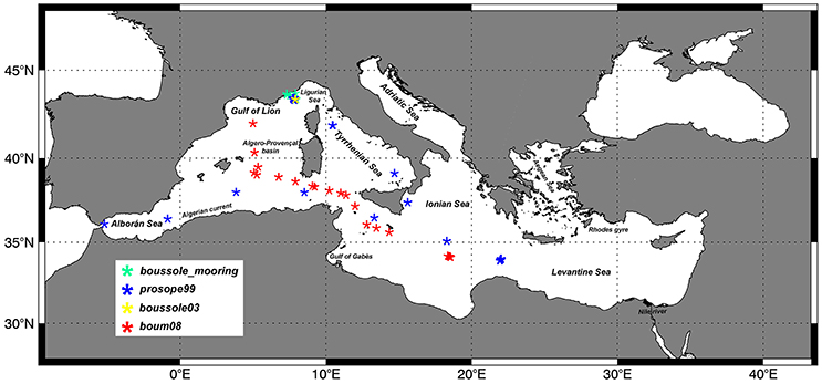
Figure 1. Spatial distribution of the phytoplankton pigments in the SeaBASS Mediterranean HPLC subset (Werdell and Bailey, 2005) used for this work.
Determination of PFTs and PSCs from Pigment Composition: Diagnostic Pigment Analysis (DPA)
Information about the composition of phytoplankton assemblage in terms of “types” and “size classes” has been obtained from the analysis of cell's pigmentary content of in-situ samples, exploiting the diagnostic properties of some marker pigments.
Following Vidussi et al. (2001), according to previous works on chemotaxonomy (Wright and Jeffrey, 1987; Gieskes et al., 1988; Everitt et al., 1990; Williams and Claustre, 1991; Claustre, 1994; Jeffrey and Vesk, 1997), we take into account seven diagnostic pigments (DPs), able to detect the main phytoplankton types and to outline the size structure of the whole assemblage in the Mediterranean Sea. Some of these pigments are unambiguous markers, others typify a principal group (with a minor contribution of some other classes, see Table 1). In Vidussi et al. (2001) the identification of the PSCs is founded on the relation between taxonomic groups and their most common dimensions in the Mediterranean Sea. Although, the phytoplankton grouping method based on the auxiliary pigments does not exactly reflect the phytoplankton size such as the one based on the size fractionated chlorophyll (lacking for the Mediterranean Sea), nevertheless several investigations about the typical off shore composition of phytoplankton Mediterranean community have proven the validity of this approach (Vidussi et al., 2001; Siokou-Frangou et al., 2010). Therefore, it must be taken into account that, on the basis of Sieburth et al. (1978) size classification, “micro” consists of Diatoms and Dinoflagellates in general, nano includes Cryptophytes, Haptophytes, and some classes of Heterokontophytes, and pico-phytoplankton is referred to Cyanobacteria, green flagellates, and Prochlorophytes (Table 1). In this work we also applied the linear adjustment of Brewin et al. (2010) for the assignment of 19′ hexanoyloxyfucoxanthin (primarily marker of the Haptophytes), more traceable to pico size class rather than to nano-phytoplankton in the ultra-oligotrophic waters (Hirata et al., 2008; Ras et al., 2008).
For the quantification of each type, a now well-established method is to estimate the contribution of different phytoplankton groups to the TChla of the whole assemblage on the basis of the pigment ratio of each marker to the TChla (Gieskes and Kraay, 1983; Gieskes et al., 1988; Barlow et al., 1993). Following this approach, Uitz et al. (2006), carried out a multiple regression analysis between the concentrations of TChla and the seven diagnostic pigments suggested by Vidussi et al. (2001), providing the best estimates of the “Total Chlorophyll a–Diagnostic Pigments” ratios (TChla/DPs) for a global data set. Applying this method, recently Di Cicco (2014) found a regional TChla–DPs relationship, based on Mediterranean data only, to evaluate the different pigment ratios of the phytoplankton assemblage that occur in this basin (Sammartino et al., 2015).
In this work, we revised this regional relationship defining new coefficients according to the new quality assurance applied to the SeaBASS data. The analysis is carried out on the 1,379 individual samples where TChla and all the seven selected biomarker pigments were available at the same time. It is important to underline that in accordance with Hooker et al. (2012) we defined TChla as the sum of Chlorophyll a with its allomers and epimers, Divinyl-Chlorophyll a, and Clorophyllide a (see Table 1).
Table 2 presents the best estimates resulting from the multiple regression analysis for the determination of the seven Mediterranean TChla/DPs ratios. The coefficients for each DP with their standard deviation and significance level are shown. The regression is highly significant, with a determination coefficient (r2) between the SeaBASS in-situ TChla and TChla estimated (TChla*, Table 3) equal to 0.99, and a p < 0.001 (based on the t-test).
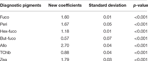
Table 2. Best estimates (new coefficients) of the “TChla to DP” ratios for the Mediterranean SeaBASS subset with their standard deviation and significance value (p-value).
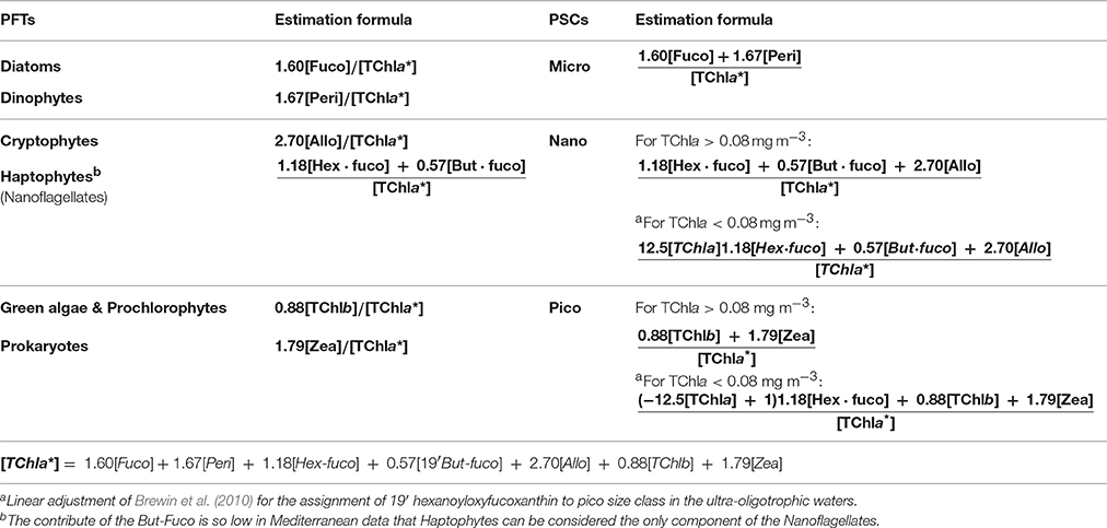
Table 3. PSCs and PFTs used in this work with their in-situ estimation formulas (fraction of TChla*, ranging from 0 to 1) resulted from the Diagnostic Pigment Analysis.
The final estimation formulas used for the in-situ quantification of each PFT and PSC fractions are schematically presented in Table 3 (each group is expressed as fraction of TChla*).
PSC and PFT Model Development
The in-situ dataset of PSC and PFT fractions resulted from the DPA has been randomly divided in two independent subsets, the first used for the model calibration (70% of the total data) and the remaining 30% for their validation. The existing co-variability founded between the accessory pigments linked to each fraction and the TChla allows the use of the latter as an index of the phytoplankton assemblage structure (Chisholm, 1992; Hirata et al., 2011). For each PFT and PSC group the relative in-situ fractions were regressed against the corresponding log10-transformed in-situ TChla concentrations (Figure 2), considering the log-normal distribution of this pigment (Campbell, 1995). We used the ordinary least square fit to define the functional forms that were better appropriate to represent the Mediterranean data distribution. Different functional forms were tested against our calibration dataset, starting from linear equation to more complex polynomial or exponential function, obviously also including the functions adopted by global PFT and PFC models. This allowed us to select the most appropriate functional forms, corresponding to those that better minimize the residual between the estimates and the observations. This results in six empirical relationships obtained by the regression technique, while the other three are derived as difference to maintain the mass balance. To obtain the TChla concentration related to each PFT and PSC group is sufficient to just multiply the fraction for the in-situ TChla.
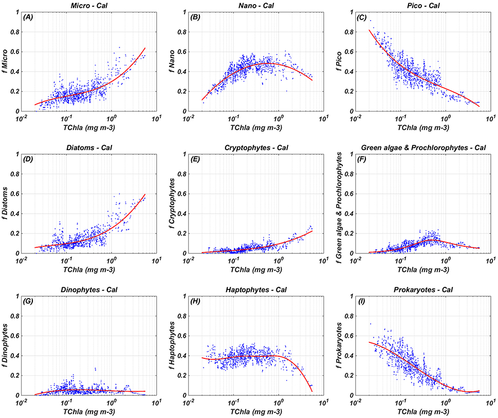
Figure 2. Regional relationships between in-situ TChla and the fraction (f) of each PSC and PFT: calibration (Cal) results. The blue dots refer to the in-situ PSC/PFT fraction obtained from equations in Table 3 (966 data) and the red line indicates the best fitting curve obtained from the calibration (see equations in Table 4). (A) Micro-Cal, (B) Nano-Cal, (C) Pico-Cal, (D) Diatoms-Cal, (E) Cryptophytes-Cal, (F) Green algae & Prochlorophytes-Cal, (G) Dinophytes-Cal, (H) Haptophytes-Cal, and (I) Prokaryotes-Cal.
Satellite Data and Processing
For the PSC and PFT determination from remote sensing we used the TChla Mediterranean reprocessed product available from Copernicus Marine Environment Monitoring Service (CMEMS, see OCEANCOLOUR_MED_CHL_L3_REP_OBSERVATIONS_009_073 product). These data were produced by the CMEMS Ocean Color Thematic Assembling Centre (OCTAC) using the ESA OC-CCI (European Space Agency—Ocean Color Climate Change Initiative) processor. MERIS, MODIS-Aqua, and SeaWiFS observations were merged into a single data by applying a series of state-of-the-art algorithms, from the atmospheric correction to the band shift correction schemes (for a comprehensive overview of the ESA-CCI products see http://www.esa-cci.org). Remote Sensing Reflectance (Rrs) spectrum is used as input to compute surface TChla (nominal resolution of 1 Km) via regional ocean color algorithm. The specific product used in this work, specialized for the Mediterranean Sea, is a merged Case 1—Case 2 product that takes into account the different optical properties of the offshore and inshore waters. Two different regional algorithms were applied on the reflectance: the MedOC4 algorithm (Volpe et al., 2007) for the case 1 waters, developed by the Group for Satellite Oceanography (GOS-ISAC) of the Italian National Research Council (CNR), and the AD4 (D'Alimonte and Zibordi, 2003), specialized for the case 2 ones. The exact identification of the two water types is performed by taking into account the whole light spectrum from blue to NIR bands for both two water types from in-situ data (D'Alimonte et al., 2003). For the waters with intermediate features, a weighted average of the two former algorithms was applied, based on the distance between the actual reflectance spectrum and the two reference reflectance spectra for case 1 and 2 waters, respectively.
For more details on the processing adopted by the data producers and the quality product assessment see Volpe et al. (2012) and http://marine.copernicus.eu/documents/QUID/CMEMS-OC-QUID-009-038to045-071-073-078-079-095-096.pdf.
In this work, we used 18 years (from 1998 to 2015) of daily TChla to compute Mediterranean daily PFT and PSC maps using the new regional algorithms described in Section Empirical Algorithms for the Identification of the PFTs and PSCs: Calibration and Validation. Daily fields were then used to build-up Mediterranean PFT and PSC climatology. Taking into account the applicability range of our models (0.02–5.52 mg m−3), in our processing we considered “good values” only the satellite TChla data falling in this range, masking the outsider.
Results
Empirical Algorithms for the Identification of the PFTs and PSCs: Calibration and Validation
The new regional algorithms with their mathematical equations and the resulting regression coefficients are showed in Table 4. Most of the considered phyto-groups are well outlined by simple polynomial functions (cubic for micro, Diatoms, Cryptophytes, and Prokaryotes and quadratic for nano), except for the class of “Green algae & Prochlorophytes,” better represented by a different equation following the approach of Hirata et al. (2011, see Table 4). These functions, shown in Table 4, are applicable over a TChla range from 0.02 to 5.52 mg m−3.
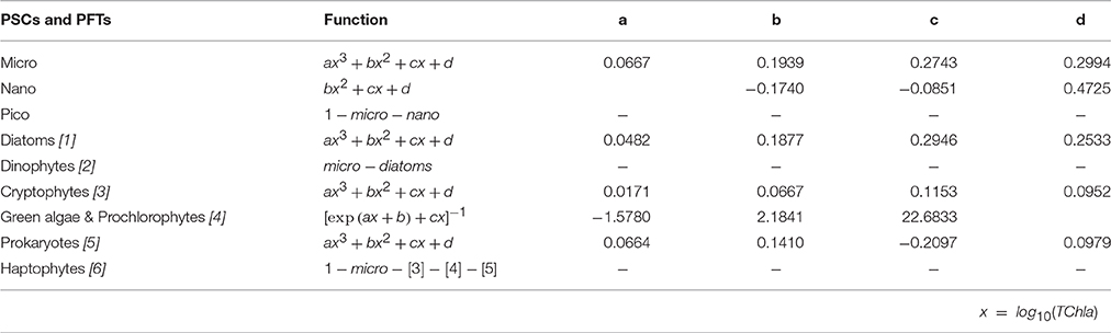
Table 4. Regional algorithms developed to estimate the PSCs and PFTs in the Mediterranean Sea (as fraction of TChla, ranging from 0 to 1). For each dimensional and functional group, the equation and its relative coefficients are given.
Figure 2 shows the results of the algorithm calibration. Micro-phytoplankton function (Figure 2A) increases monotonically with the increase of the TChla, ranging from the 8% to the 63% of the TChla concentration. Pico equation (Figure 2C), instead, shows an opposite behavior, with minimum and maximum values for maximum and minimum TChla concentrations, respectively, ranging between 5 and 81% of TChla. The nano function (Figure 2B) presents an intermediate trend, ranging from 12 to 48% of TChla, with a maximum in correspondence of about 0.57 mg m−3 of TChla. The micro component consists almost entirely of the Diatom group contribution, represented by a cubic function (Figure 2D) similar to the micro one, increasing monotonically with the TChla too. The contribution of the Dinophytes (Figure 2G) to the micro component and to the TChla concentration is very low, with a small range of variation between 1 and 6% of TChla, indicating that diatoms are the major constituent of the micro-phytoplankton in the Mediterranean Sea. Prokaryotes curve (Figure 2I) decreases monotonically from 55 to 3%, co-varying with the TChla increase. At lower chlorophyll concentrations Prokaryotes represents the main component of the pico group (with the contribution of small Haptophytes in the ultra-oligotrophic water). Increasing the chlorophyll value, the non-monotonic signal of the “Green algae & Prochlorophytes” (Figure 2F) grows up to the maximum value (about 13%) in correspondence of the TChla concentration of about 0.5 mg m−3. For higher value of TChla the function decreases with a weaker slope, concurring to the pico group more than to the Prokaryotes. Also the Cryptophytes (Figure 2E) co-vary with the TChla, growing up with the increment of this pigment from a minimum of 1% to a maximum of 22% at higher TChla values. At last but not least in terms of relative contribution to the TChla, the Coccolithophores curve (Figure 2H) presents a small range of variation (35–40%) for almost the entire range of chlorophyll, decreasing up to a minimum value about 10% at maxima TChla concentrations (about 5 mg m−3).
The results of the application of the Mediterranean algorithms (Table 4) on the validation dataset are shown in Figures 3, 4 (right panels), for the PSCs and the PFTs, respectively. The scatter plots of the TChla, estimated for each class applying the algorithms against the observed TChla fractions, clearly show the goodness of the fits for all the considered groups. The data points are uniformly distributed around the 1:1 line with a very narrow scatter.
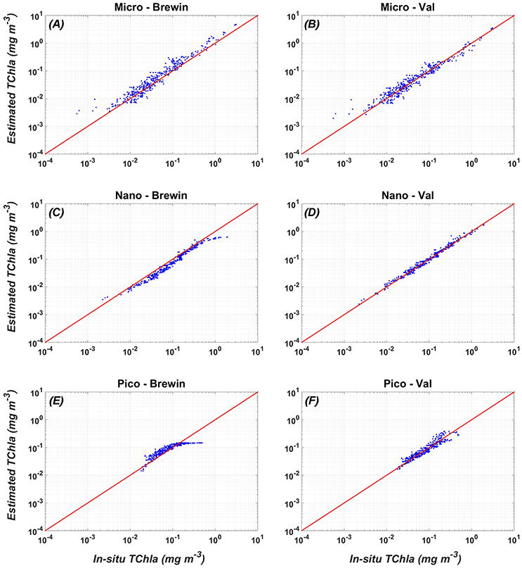
Figure 3. Comparison between the validation (in-situ vs. estimated PSC TChla concentrations) of the new PSC regional algorithms (Val, right panel: B,D,F) vs. the global PSCs model of Brewin et al. (2011) (Brewin, left panel: A,C,E). For the statistics, see Table 7.
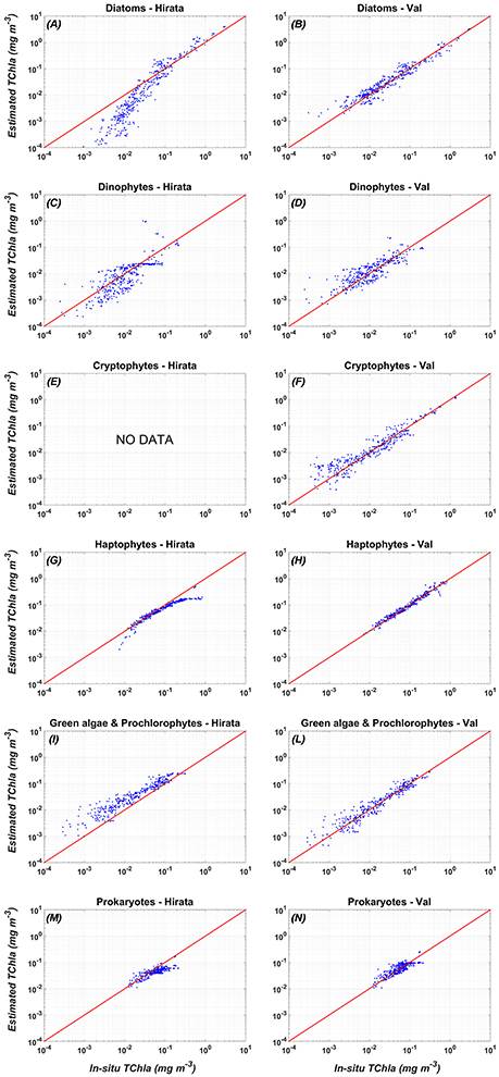
Figure 4. Comparison between the validation of the new PFT regional algorithms (Val, right panel: B,D,F,H,L,N) vs. the global PFT model of Hirata et al. (2011) (Hirata, left panel: A,C,E,G,I,M): in-situ (x axis) vs. estimated (y-axis) PFT TChla concentrations. (A) Diatoms-Hirata, (B) Diatoms-Val, (C) Dinophytes-Hirata, (D) Dinophytes-Val, (E) Cryptophytes-Hirata, (F) Cryptophytes-Val, (G) Haptophytes-Hirata, (H) Haptophytes-Val, (I) Green algae & Prochlorophytes-Hirata, (L) Green algae & Prochlorophytes - Val, (M) Prokaryotes - Hirata, (N) Prokaryotes - Val. For the statistics, see Table 7.
A more quantitative evaluation of the proposed algorithm performances comes from the computation of the mean absolute error (root mean squared error, RMSE) and other statistical parameters (see Table 5 for the relative reference equations) with respect to the original PSC and PFT in-situ data (Table 6, calibration; Table 7, validation). A hindcast evaluation of the algorithm performances was also carried out (i.e., the same calibration data were used for fitting and testing). Furthermore, the error relative to the new regional algorithms is compared to the error associated with global abundance-based models applying them to the same validation dataset (Table 7). In particular, we used the empirical global relationships of Hirata et al. (2011), the only ones based on the abundance which are focused also on the PFTs, and the Brewin et al. (2010) models, applying the coefficients recalibrated in Brewin et al. (2011), developed only for the PSCs.
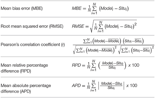
Table 5. Mathematical equations used to compute the statistic parameters.
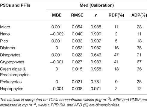
Table 6. Statistical results of the new regional algorithms (Med) applied to the calibration dataset (70% of the entire subset = 966 data).
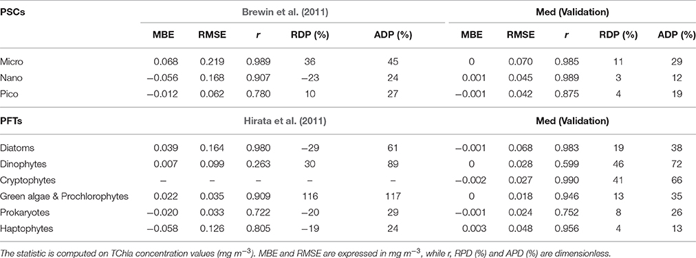
Table 7. Statistical results of the new regional algorithms (Med) validation compared with the statistics resulting by applying the global models (Brewin et al., 2011; Hirata et al., 2011) on the same validation dataset (30% of the entire subset = 413 data).
The new regional algorithms show good performances for most of the groups taken into account (Table 6, calibration; Table 7, validation). The results obtained applying the algorithms to the validation dataset are consistent with the hindcast evaluation. Pearson correlation coefficient, which gives an estimate of the covariance between the models and the in-situ validation data, shows high correlation, with values ranging from 0.75 to 0.99 both for PSCs and PFTs, excluding the group of the Dinophytes (r = 0.60), probably also because of this group is derived as difference. All groups show very low values of mean bias error (MBE), ranging from −0.002 to 0.003 mg m−3 for the validation dataset. The RMSE, which gives a measure of the spread of the estimated values around the in-situ observed ones, goes from 0.018 mg m−3 for the “Green algae & Prochlorophytes” to 0.068 mg m−3 for the Diatoms in the PFT group and from 0.042 mg m−3 for the pico- to 0.070 mg m−3 for the micro-phytoplankton in the PSCs.
The comparison of the scatter plot obtained by the application of the PSC regional models with respect to the global models (Figure 3) shows that the Mediterranean algorithms perform better than the global ones for all the three groups. This evidence is confirmed by the statistical analysis (Tables 6, 7). Although, the Brewin et al. (2011) models applied to the Mediterranean data show high values of the correlation coefficient (0.9 for micro- and nano-phytoplankton), the statistical results highlighted that the regionalization improves the uncertainty (MBE) and the spread (RMSE) of about one order of magnitude for all the size classes. For example, for the micro-phytoplankton the MBE decreases from 0.068 to 0 when the regional algorithm is applied. In particular, the Brewin's algorithm slightly overestimates the micro component (Figure 3A) in the entire dynamical range of concentration. The behavior of this global model is exactly the opposite for the nano class, always underestimating the observed values (Figure 3C) resulting into a MBE of −0.056. As consequence, the main trend is the overestimation of the pico-phytoplankton component for concentrations lower than 0.1 mg m−3, and the underestimation at greater values (Figure 3E).
Figure 4 shows that applying the global models of Hirata et al. (2011) to the Mediterranean data Prokaryotes (Figure 4M), Haptophytes (Figure 4G), and Diatoms (Figure 4A) would be underestimated. This underestimation results into a mean relative percentage difference, RPD, of −20, −19, and −29%, respectively. The “Green algae & Prochlorophytes” (Figure 4I), instead, are overestimated (RDP = 116%). The predictive power for the Dinophytes (Figure 4C) is negligible, as in the global validation of the model (see (Hirata et al., 2011) for more details), with an r = 0.26 (Table 7). It must be taken into account that, unlike to this work, the development of the models of Diatoms and Haptophytes in Hirata et al. (2011) is based on in-situ Fuco and Hex-fuco data at which a background correction was applied. The Fuco signal in oligotrophic waters (<0.25 mg m−3) is assumed to be due to smaller Haptophytes rather than Diatoms. This correction is significant only at lower TChla concentrations. It means that, applying this global model in this TChla range, the estimates of Diatoms could be slightly improved for the Mediterranean Sea but, at the same time, the estimates of the Haptophytes would get worse. As for the PSCs, also for the PFTs (Figure 4) the regionalization reduces the bias of about one order of magnitude for all the types (Tables 6, 7). The preliminary analysis of r, MBE, and RMSE has showed a very good predictive power for all the new regional models. The best performances seem to be associated with the algorithms of Cryptophytes and “Green algae & Prochlorophytes” for the PFTs, followed by Haptophytes and Diatoms, and with the nano model for the PSC group. The study of the RPD and the mean absolute percentage difference, APD, has integrated this statistic information, taking also into account the different dynamical range of the TChla concentration represented by each class. Weighing the uncertainty on the dynamical range of the observed concentration values, statistical data confirmed the goodness of the fits for all the phytoplankton groups (Table 7) and showed the best predicted power for the algorithms which estimate the nano (RDP = 3% and ADP = 12%) and Haptophytes (RDP = 4% and ADP = 13%) components, for PSCs and PFTs, respectively. These considerations are also confirmed by the validation results represented in Figures 3, 4.
Application of the New Regional Algorithms to the Daily Mediterranean Reprocessed TChla CASE1–2 Time Series: PSC and PFT Climatology (1998–2015)
The new regional algorithms (Table 4) are applied on an 18 years' time series of TChla satellite estimates (see Section Data and Methods) to compute PSCs and PFTs. Figures 5, 6 show annual PSC and PFT (1998–2015) climatology, respectively. In the left panel, each map shows the fractions of the TChla represented by each phytoplankton component. For each pixel the percentage maps give fraction values relative to the chlorophyll concentration (Figure 5, top panel), whose distribution is typically characterized by a West–East decreasing gradient in the Mediterranean Sea (Siokou-Frangou et al., 2010; Estrada and Vaqué, 2014). In the right panel, instead, the maps show the relevance of each class in terms of TChla estimates (mg m−3).
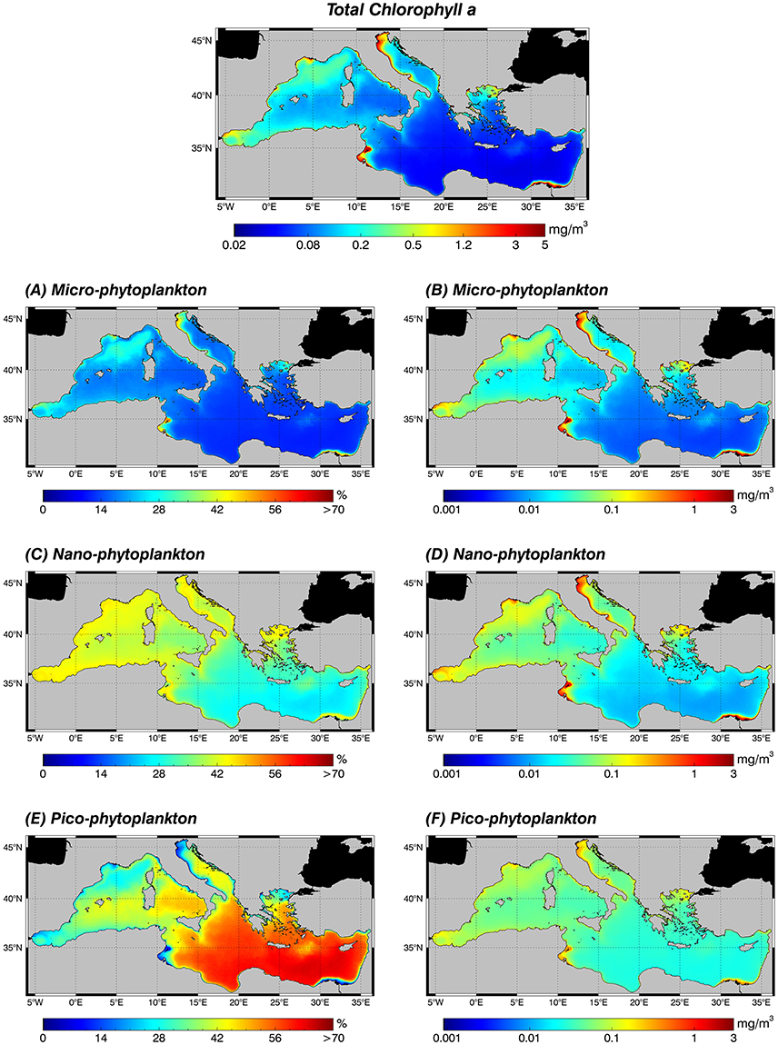
Figure 5. Annual climatological maps (1998–2015) of the TChla (top panel) and the PSCs: for each pixel, fractions are expressed in % with respect to the TChla (left panel: A,C,E) and the contribution of each PSC group to the TChla concentration in mg m−3 (right panel: B,D,F). PSCs are retrieved applying the new regional algorithms (see Table 4) on the daily TChla times series (Mediterranean reprocessed product produced by the CMEMS-OCTAC). (A,B) Micro-phytoplankton, (C,D) Nano-phytoplankton, (E,F) Pico-phytoplankton.
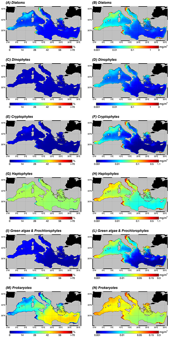
Figure 6. Annual climatological maps (1998–2015) of the PFTs: for each pixel, fractions are expressed in % with respect to the TChla (left panel: A,C,E,G,I,M) and the contribution of each PFT group to the TChla concentration in mg m−3 (right panel: B,D,F,H,L,N). PFTs are retrieved applying the new regional algorithms (see Table 4) on the daily TChla time series (Mediterranean reprocessed product produced by the CMEMS-OCTAC). Since the wide range of TChla variability related to each PFT, note that the color scales could be different. (A,B) Diatoms, (C,D) Dinophytes, (E,F) Cryptophytes, (G,H) Haptophytes, (I,L) Green algae & Prochlorophytes, (M,N) Prokaryotes.
All the three size classes reach their maxima absolute values, >3 mg m−3 of TChla for micro (Figure 5B), and about 1.6 and 0.4 mg m−3 for nano (Figure 5D) and pico (Figure 5F), respectively, in the more productive zones of the basin (see Figure 5, top panel). In the eastern basin these areas are: the North Adriatic Sea and in general the whole Adriatic coast (due to the great nutrient supply from the Po river); the south-eastern area of the Levantine basin influenced by the outflow of the Nile river; the Northern Aegean Sea and the Gulf of Gabès (probably only an area of very shallow water). Otherwise, in the western basin, these more productive regions are the Gulf of Lion, the eastern cost of Spain, and the Tyrrhenian Sea coast. Very high values (greatest for the nano class) are also evident in the North–western Alborán Sea and along the Algerian and Tunisian coasts up to the Sicily channel, in the Liguro-Provençal and part of the Catalan Basin and in the cyclonic area of the North Tyrrhenian Sea. As expected, the existing co-variability between the accessory pigments linked to each fraction and the TChla is highlighted by the percentage maps (Figure 5, left panel). In the more oligotrophic eastern Mediterranean Sea, where TChla climatology shows the lower absolute concentrations (Figure 5, top panel), the relative dominant component is the pico class (Figure 5E). Here, the TChla concentration of the pico-phytoplankton (Figure 5F) is about five times micro (Figure 5B) and two times the nano one (Figure 5D). On the contrary, in the regions where the TChla reaches higher values, the percentage contribution of the nano and micro components increase (Figures 5A,C, respectively). Generally, in the whole basin the nano component shows intermediate values, in particular ranging from 30 to 40% of the TChla in the western basin, growing up to 45% in highly productive areas (Figure 5C).
Moving to the PFTs, the abundance of each class in terms of TChla concentration (Figure 6, right panel) reflects, as occurred in the size classes, the gradient of this pigment (Figure 5, top panel), showing for all groups higher values in the western basin and in the already mentioned high productive zones of the entire basin. This is true for all groups. In the climatological analysis, Prokaryotes constitute the principal component of the pico-phytoplankton in almost all areas, both in terms of percentage (Figure 6M) and concentration (Figure 6N). They are the absolute dominant group in the oligotrophic and ultra-oligotrophic waters of the eastern basin, but also for the western basin in the southern Tyrrhenian Sea and in some areas of the Algero-Provençal basin (Figure 6M). In the Levantine basin the second group in terms of TChla concentration is the Haptophytes (Figure 6H). They represent the dominant class within the nano-phytoplankton in the whole Mediterranean Sea and constitute the main group featuring the case 1 water of the western basin (Figure 6G). Diatoms (Figures 6A,B) dominate in the micro-phytoplankton and can be considered the third group in terms of TChla concentration in the open sea, followed by the Green algae (Figure 6L), Cryptophytes (Figure 6F) and, finally, Dinoflagellates (Figure 6D). Otherwise, in coastal areas Diatoms dominate, reaching values about of 3 mg m−3. This is well-evident in the North Adriatic Sea and in general in the entire Adriatic coast, in the southeastern area of the Levantine basin influenced by the outflow of the Nile River and in the Gulf of Gabès (Figure 6B). In general, in terms of chlorophyll concentration, in the coastal areas we find the predominance of the Diatoms and Haptophytes, followed by the remaining classes (Figure 6, right panel).
At last but not least in terms of biological importance, the phytoplankton distribution in the Alborán Sea and along the Algerian-Tunisian coasts is characterized by the dominance of the Haptophytes, followed by Diatoms, and then Prokaryotes, Green algae, Cryptophytes, and at last Dinoflagellates.
In addition, in Figure 7 we show the results of the monthly climatology of each group, averaged over the whole Mediterranean Sea. On basin scale, the component mostly representative of the TChla seems to be the nano-phytoplankton for the PSCs (top panel), especially in the bloom periods typical of the midlatituds. Nano is followed by pico and the component with the lower contribution to the TChla is the micro one. Only in summer, pico-phytoplankton dominates on the TChla concentration, exceeding the other two classes. In the same season, the micro component reaches its minimum values. The monthly mean PFT climatology (Figure 7, bottom panel) confirms the predominance of the Haptophytes within the nano-phytoplankton in the whole Mediterranean Sea as highlighted in the previous PFT map analysis (Figure 6H). This is also the predominant group all over the year. The Haptophytes are followed by Diatoms and Prokaryotes representing the main component for the micro- and the pico-phytoplankton, respectively. More in detail, the contribute of the Diatoms to the TChla concentration is greater than the Prokaryotes only in the early spring. The two classes show similar concentrations in late autumn and winter season while, in the remaining part of the year, Prokaryotes dominate. Cryptophytes and “Green algae & Prochlorophytes” always reveal a same contribution, even if the concentration of the latter is slightly greater in late winter—early spring. These two functional groups represent the smallest fractions within the nano- and pico- size classes, respectively. At last, Dinophytes constitute the class with the lowest TChla concentration all over the year.
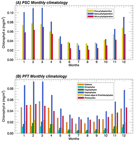
Figure 7. Mean monthly climatology (1998–2015) of the PSCs (A) and the PFTs (B) over the Mediterranean Sea in terms of their contribution to the TChla (mg m−3). The PSCs and PFTs are retrieved applying the new regional algorithms (see Table 4) on the daily Total Chlorophyll a time series (Mediterranean reprocessed product produced by the CMEMS-OCTAC).
Discussion and Conclusions
The Mediterranean Sea is typically characterized by peculiar optical properties that make its color different from the global ocean (Volpe et al., 2007). In addition to an abundant aerosol dominated by continental anthropogenic pollution (Moulin et al., 1997) and the presence of Saharan dust in the water column (Claustre et al., 2002), one of the main reasons that justifies its color seems to be a different phytoplankton assemblage structure typical of this basin (Volpe et al., 2007). This is also confirmed by the presence of pigment ratios different with respect to those of the global ocean (Sammartino et al., 2015). This implies the need of regional algorithms that take into account all these peculiar characteristics. In the last year, several specialized algorithms have been proposed for the detection of the chlorophyll a concentration (e.g., Volpe et al., 2007; Santoleri et al., 2008). Instead, PFT and PSC regional algorithms do not exist, except for the recent work of Navarro et al. (2014). They adapted the previous version of the PHYSAT method of Alvain et al. (2005, 2008), providing regional estimates of dominant PFT groups. In our work, for the first time, new regional algorithms have been advanced to identify, together, the contribution of each PSC and PFT group to the satellite estimates of TChla concentration. This different approach, based on the close link existing between the abundance of each group and the trophic status of the environment (Margalef, 1967, 1978; Brewin, 2011), provides new kind of information, complementary to the results of the PHYSAT-Med.
Our assessment of the uncertainty associated to the new developed regional algorithms and the most used global models based on the same approach, highlight and confirm that a regionalization for the PSC and PFT satellite algorithms is required. As shown by our validation results (Section Empirical Algorithms for the Identification of the PFTs and PSCs: Calibration and Validation), the use of Mediterranean PSC and PFT algorithms allowed to eliminate the bias between observations and estimates and to reduce the RMSE of an order of magnitude respect the global models.
Even if the uneven distribution of the in-situ observations between western-central Mediterranean Sea and the eastern basin could imply that the new formulations are more appropriate for the western basin, we are confident that the derived parameterizations can be applied also in the eastern Mediterranean Sea without introducing a significant bias on satellite estimates. In fact, the in-situ dataset used for the algorithm calibration includes the typical values of chlorophyll a observed in the oligotrophic waters of eastern Mediterranean Sea (ranging from 0.02 to 0.14 mg m−3). The number of the samples that fall in this chlorophyll range represent the 38% of the total number of the calibration data, 18% of which are acquired in the eastern Mediterranean Sea. This implies that the oligotrophic condition is well represented in our dataset. For a further assessment, we made a preliminary evaluation of the new parameterizations limited to the eastern Mediterranean Sea using all available in-situ observation in our dataset. This results into a bias (from −0.001 to 0.001 depending on the PFT/PCS parameterization) and RMS (from 0.002 to 0.004 depending on the PFT/PCS parameterization), values comparable with the bias obtained in western Mediterranean for the same TChla range and with the values resulting from the algorithm validation (see Table 7). Even if this result cannot be considered conclusive since has been obtained with a limited number of in-situ observations, the statistical results seem to indicate that our parameterization should not introduce any significant bias to satellite derived estimates.
The analysis of the phytoplankton assemblage distribution patterns resulted from the application of our new algorithms to the Mediterranean multi-sensor reprocessed dataset (1998–2015) is consistent with the main previous knowledge, both in terms of distribution and phytoplankton ecology (Siokou-Frangou et al., 2010; Uitz et al., 2012; Estrada and Vaqué, 2014; Navarro et al., 2014). Pico-phytoplankton, with Prokaryotes as the main component, is widespread throughout the whole basin and always dominant in oligotrophic and stratified waters (see Section Results) in agreement with the observation of Siokou-Frangou et al. (2010), according to which the pico component constitutes more than 50% of the total biomass in these conditions (Estrada and Vaqué, 2014). Furthermore, our results show that pico class reaches its maximum value (about 0.4 mg m−3) in the more productive areas. These considerations are also in consonance with ecological behavior and strategy of this group. Size affects nutrient solute and water fluxes across the plasmalemma, favoring the smaller sized cells in the oligotrophic water. This is due to the larger surface to volume ratio of small cells with respect to the larger ones, which make the former efficient nutrient absorber in very low nutrient conditions. Moreover, in stratified environments the probability of sinking out from the euphotic zone is greater in the micro-sized cells than in the smaller ones, undergoing a lower loss of organisms (Chisholm, 1992; Raven, 1998). However, this does not imply that Prokaryotes and pico-phytoplankton in general reach the maxima values in terms of chlorophyll concentration in the oligotrophic conditions. In fact, Chisholm (1992) suggested that they usually achieve their “maximum potential biomass” (of about 0.5 mg m−3) in high nutrient conditions, in accordance with our estimates. We showed that, in the more productive region of the basin, the chlorophyll concentrations of the pico and Prokaryotes classes correspond to relative small percentage of TChla (Chisholm, 1992). Indeed, our climatological maps shows the dominance, in these conditions, of the micro component with values that exceeds up to the 50% of the TChla, followed by nano- and, at last, by a minor contribute of the pico-phytoplankton (about 10–15%).
Within the micro group, the major contribute is clearly due to the Diatoms in the higher nutrient areas. This is justified by the ecological strategy of this functional group, physiologically better adapted to high dynamic conditions and more efficient in the nutrient absorption. Moreover, they are also able to subtract nutrients from the surrounding environment and to store them in their large vacuoles, depriving other groups and supporting their growth at the same time (Margalef, 1978; Falkowski et al., 2003; Litchman et al., 2007; Estrada and Vaqué, 2014). About the Dinoflagellates, their contribution to the micro-phytoplankton is very low with respect to the Diatoms one. This is probably due to their different ecological strategy, well-adapted to high dynamical environment but with a higher affinity for low nutrient conditions. Moreover, Estrada and Vaqué (2014) suggested that the use of peridinin as biomarker pigment for the Dinoflagellates identification could cause an underestimation of their abundance because it could be not present in some organisms of this class (Jeffrey and Vesk, 1997).
An important result of this study is the information on the Nanoflagellate distribution, mainly represented by the Haptophytes in our dataset. This can represent a precious novelty, considering the lack of knowledge on the Nanoflagellate spatial distribution, improved only in the last years thanks to the more diffused usage of chemotaxonomic and molecular techniques (Latasa et al., 2010). The widespread distribution of the nano component and its high contribution to the TChla in the whole basin confirms the Uitz et al. (2012) results, according to which the primary production in the Mediterranean Sea is mainly due to the nano-phytoplankton component.
The lack of data on the phytoplankton biogeography at different spatio-temporal scales in the whole Mediterranean Sea and the well-known difficulties in the long-term acquisition of in-situ data at basin scale make essential the use of the remote sensing technique for a synoptic observation of the phytoplankton assemblage composition and its diversity. Our analysis revealed the importance of providing regional algorithms strictly required to suit the peculiar bio-optical properties featuring this basin. The statistical results demonstrated the goodness of the performance and the applicability of our models for the abundance estimations of PSCs and PFTs together.
Nowadays, in the context of international Climate Change Initiatives and cooperation, a synergic effort of the Space Agencies in collaboration with remote sensing scientist is conducted to identify the major gaps (both instrumental and scientific) that should be filled to improve the accuracy of satellite estimates of the phytoplankton groups and their variability (Bracher et al., 2017). In this framework, the following actions summarize our future perspectives to improve remote observations on the Mediterranean Sea: (a) to extend the validation and calibration of the PFT new regional algorithms including new in-situ dataset of HPLC Total Chlorophyll a and diagnostic pigments acquired, in recent years, by the Mediterranean scientific community; (b) to improve the accuracy of the PSC algorithms with a new calibration and validation only based on TChla size-fractions; (c) to carry on the in-situ bio-optical measurements to cover all the un-sampled Mediterranean regions, also with the intent to exploit different approaches (e.g., spectral response-based); (d) to extend this regionalization activity to new generation sensors (e.g., OLCI for Sentinel-3) to obtain higher resolution information also for phytoplankton dynamical studies at mesoscale; (e) to analyse the Mediterranean PFT and PSC trends, thanks to the availability of consistent long term satellite observation time series.
On time scales larger than the period we considered, climate or human induced changes in environmental conditions can produce modifications of phytoplankton pigment composition and thus the pigment ratios to the Total chlorophyll a. This implies that the simple empirical relations used to compute the PFTs and PFCs from the chlorophyll observations need to be re-evaluated and or a more sophisticated approach which links the pigment ratios, the PFT, and PSC composition and the major environmental forcing should be developed.
Author Contributions
All the authors contributed to the conception and design of the work and approved the final version of the manuscript to publish. AD carried out the work, performing the Diagnostic Pigment Analysis, the algorithm development and their analysis supported by the experience of RS and SM and drafting the most of the manuscript. MS processed the satellite data, developed all the climatological maps and edited all the images of the manuscript. MS, SM, and RS revised critically the manuscript and contributed to its draft.
Funding
This research was supported by the European Commission in the framework of the Copernicus Marine Environmental Services—Ocean Color Thematic Assembling Center Project (Grant agreement 9836100). The research was also supported by the “Ministero dell'Istruzione, dell'Università e della Ricerca” in the framework of the Italian Flagship Project RITMARE (la Ricerca ITaliana per il MARE).
Conflict of Interest Statement
The authors declare that the research was conducted in the absence of any commercial or financial relationships that could be construed as a potential conflict of interest.
Acknowledgments
The authors would like to thank the OC-CCI and CMEMS Project that generated the satellite chlorophyll data used in this paper, which are free available at http://marine.copernicus.eu/. We also acknowledge the SeaBASS archive for the in-situ bio-optical dataset, free available at https://seabass.gsfc.nasa.gov/. We want to thank ESA/ESRIN for the “Phytoplankton Diversity at Global and Regional Scale” session, within the “Color and Light from Earth Observation” (CLEO) workshop. We are grateful to Simone Colella for his invaluable scientific and technical advices. This work also benefited from discussions with Alessio Ansuini, Vittorio Brando, Riccardo Droghei, Marco Picone, Jaime Pitarch Portero, and Gianluca Volpe. We also would like to thank Vega Forneris and Flavio La Padula for their valuable technical support.
References
Aiken, J., Pradhan, Y., Barlow, R., Lavender, S., Poulton, A., Holligan, P., et al. (2009). Phytoplankton pigments and functional types in the Atlantic Ocean: a decadal assessment, 1995-2005. Deep Sea Res. II 56, 899–917. doi: 10.1016/j.dsr2.2008.09.017
Alvain, S., Moulin, C., Dandonneau, Y., and Bréon, F. M. (2005). Remote sensing of phytoplankton groups in case 1 waters from global SeaWiFS imagery. Deep Sea Res. I 52, 1989–2004. doi: 10.1016/j.dsr.2005.06.015
Alvain, S., Moulin, C., Dandonneau, Y., and Loisel, H. (2008). Seasonal distribution and succession of dominant phytoplankton groups in the global ocean: a satellite view. Global Biogeochem. Cycles 22:GB3001. doi: 10.1029/2007GB003154
Barlow, R. G., Mantoura, R. F. C., Gough, M. A., and Fileman, T. W. (1993). Pigment signatures of the phytoplankton composition in the northeastern Atlantic during the 1990 spring bloom. Deep Sea Res II 40, 459–477. doi: 10.1016/0967-0645(93)90027-K
Basset, A., Sangiorgio, F., and Pinna, M. (2004). Monitoring with benthic macroinvertebrate: advantage and disadvantages of body size descriptors. Aquat. Conserv 14, S43–S58. doi: 10.1002/aqc.649
Blondel, J. (2003). Guilds or functional groups: does it matter? Oikos 100, 223–231. doi: 10.1034/j.1600-0706.2003.12152.x
Bracher, A., Bouman, H., Brewin, R. J. W., Bricaud, A., Brotas, V., Ciotti, A. M., et al. (2017). Obtaining phytoplankton diversity from ocean color: a scientific roadmap for future development. Front. Mar. Sci. 4:55. doi: 10.3389/fmars.2017.00055
Brewin, R. J., Sathyendranath, S., Hirata, T., Lavender, S. J., Barciela, R. M., and Hardman-Mountford, N. J. (2010). A three-component model of phytoplankton size class for the Atlantic Ocean. Ecol. Modell. 221, 1472–1483. doi: 10.1016/j.ecolmodel.2010.02.014
Brewin, R. J. W. (2011). Detecting Phytoplankton size Class Using Satellite Earth Observation. Ph.D. Thesis, University of Plymouth.
Brewin, R. J. W., Devred, E., Sathyendranath, S., Lavender, S. J., and Hardman-Mountford, N. J. (2011). Model of phytoplankton absorption based on three size classes, Appl. Opt. 50, 4353–4364. doi: 10.1364/AO.50.004535
Brown, J. H., Gillooly, J. F., Allen, A. P., Savage, V. M., and West, G. B. (2004). Toward a metabolic theory of ecology. Ecology 85, 1771–1789. doi: 10.1890/03-9000
Brunet, C., and Mangoni, O. (2010). “Determinazione quali-quantitativa dei pigmenti fitoplanctonici mediante HPLC,” in Metodologie di Studio del Plancton Marino, Manuali e linee guida 56/2010, eds G. Socal, I. Buttino, M. Cabrini, O. Mangoni, A. Penna, and C. Totti (Rome: ISPRA), 379–387.
Campbell, J. W. (1995). The lognormal distribution as a model for bio-optical variability in the sea. J. Geophys. Res. 100, 13237–13254. doi: 10.1029/95JC00458
Chisholm, S. W. (1992). “Phytoplankton size,” in Primary Productivity and Biogeochemical Cycles in the Sea, eds P. G. Falkowski and A. D. Woodhead (New York, NY: Plenum Press), 213–237.
Ciotti, A. M., and Bricaud, A. (2006). Retrievals of a size parameter for phytoplankton and spectral light absorption by coloured detrital matter from water-leaving radiances at SeaWiFS channels in a continental shelf off Brazil. Limnol. Oceanogr. Methods 4, 237–253. doi: 10.4319/lom.2006.4.237
Ciotti, A. M., Lewis, M. R., and Cullen, J. J. (2002). Assessment of the relationships between dominant cell size in natural phytoplankton communities and the spectral shape of the absorption coefficient. Limnol. Oceanogr. 47, 404–417. doi: 10.4319/lo.2002.47.2.0404
Claustre, H. (1994). The trophic status of various oceanic provinces as revealed bv phytoplankton pigment signatures. Limnol. Oceanogr. 39, 1206–1210. doi: 10.4319/lo.1994.39.5.1206
Claustre, H., Morel, A., Hooker, S. B., Babin, M., Antoine, D., Oubelkheir, K., et al. (2002). Is desert dustmaking oligotrophic waters greener? Geophys. Res. Lett. 29, 107.1–107.4. doi: 10.1029/2001GL014056
D'Alimonte, D., Mélin, F., Zibordi, G., and Berthon, J.-F. (2003). Use of the novelty detection technique to identify the range of applicability of the empirical ocean color algorithms. IEEE Trans. Geosci. Remote Sens. 41, 2833–2843. doi: 10.1109/TGRS.2003.818020
D'Alimonte, D., and Zibordi, G. (2003). Phytoplankton determination in an optically complex coastal region using a multilayer perceptron neural network. IEEE Trans. Geosci. Remote Sens. 41, 2861–2868. doi: 10.1109/TGRS.2003.817682
Delwiche, C. (1999). Tracing the thread of plastid diversity through the tapestry of life. Am. Nat. 154, 164–177. doi: 10.1086/303291
Devlin, M., Best, M., Coates, D., Bresnan, E., O'Boyle, S., Park, R., et al. (2007). Establishing boundary classes for the classification of UK marine waters using phytoplankton communities. Mar. Pollut. Bull. 55, 91–103. doi: 10.1016/j.marpolbul.2006.09.018
Devred, E., Sathyendranath, S., Stuart, V., Maas, H., Ulloa, O., and Platt, T. (2006). A two-component model of phytoplankton absorption in the open ocean: theory and applications. J. Geophys. Res. 111:C03011. doi: 10.1029/2005JC002880
Di Cicco, A. (2014). Spatial and Temporal Variability of Dominant Phytoplankton Size Classes in the Mediterranean Sea from Remote Sensing. Ph.D. thesis in Ecology and Management of Biological Resources, Tuscia University.
Estrada, M., and Vaqué, D. (2014). “Microbial components,” in The Mediterranean Sea, Its History and Present Challenges, eds S. Goffredo and Z. Dubinsky (New York, NY, London: Springer), 87–111.
Everitt, D. A., Wright, S. W., Volkman, J. K., Thomas, D. P., and Lindstrom, E. J. (1990). Phytoplankton community compositions in the western equatorial Pacific determined from chlorophyll and carotenoid pigment distributions. Deep-Sea Res. 37, 975–997. doi: 10.1016/0198-0149(90)90106-6
Falkowski, P. G., Laws, E. A., Barber, R. T., and Murray, J. W. (2003). “Chapter 4: Phytoplankton and their role in primary, new, and export production,” in Ocean Biogeochemistry: A Synthesis of the Joint Global Ocean Flux Study (JGOFS), Global change–the IGBP series, ed J. R. Michael Fasham (Berlin; Heidelberg: Springer-Verlag), 1619–2435.
Falkowski, P. G., and Raven, J. A. (1997). Aquatic Photosynthesis. Oxford: Blackwell Scientific Publishers.
Gieskes, W. W. C., and Kraay, G. W. (1983). Dominance of Cryptophyceae during the phytoplankton spring bloom in the central North Sea detected by HPLC analysis of pigments. Mar. Biol. 75, 179–185. doi: 10.1007/BF00406000
Gieskes, W. W. C., Kraay, G. W., Nontji, A., and Setiapermana, D. (1988). Monsoonal alternation of a mixed and a layered structure in the phytoplankton of the euphotic zone of the Banda Sea (Indonesia): a mathematical analysis of algal pigment fingerprints. Neth. J. Sea Res. 22, 123–137. doi: 10.1016/0077-7579(88)90016-6
Hirata, T., Aiken, J., Hardman-Mountford, N., Smyth, T. J., and Barlow, R. G. (2008). An absorption model to determine phytoplankton size classes from satellite ocean colour. Remote Sens. Environ. 112, 3153–3159. doi: 10.1016/j.rse.2008.03.011
Hirata, T., Hardman-Mountford, N. J., Brewin, R. J. W., Aiken, J., Barlow, R., Suzuki, K., et al. (2011). Synoptic relationships between surface Chlorophyll-a and diagnostic pigments specific to phytoplankton functional types. Biogeosciences 8, 311–327. doi: 10.5194/bg-8-311-2011
Hooker, S. B., Clementson, L., Thomas, C. S., Schlüter, L., Allerup, M., Ras, J., et al. (2012). The Fifth SeaWiFS HPLC 779 Analysis Round-Robin Experiment (SeaHARRE-5). Greenbelt, MD: NASA Tech. Memo 780 2012–217503, NASA Goddard Space Flight Center, 98.
IOCCG (2014). “Phytoplankton functional types from space,” in Reports of the International Ocean-Colour Coordinating Group, No. 15, ed S. Sathyendranath (Dartmouth, NS: IOCCG).
Jeffrey, S. W., and Vesk, M. (1997). “Introduction to marine phytoplankton and their pigment signatures,” in Phytoplankton Pigments in Oceanography: Guidelines to Modern Methods, eds S. W. Jeffrey, R. F. C. Mantoura, and S. W. Wright (Paris: UNESCO), 37–84.
Kostadinov, T. S., Siegel, D. A., and Maritorena, S. (2009). Retrieval of the particle size distribution from satellite ocean color observations. J. Geophys. Res. 114, C09015. doi: 10.1029/2009JC005303
Lacombe, H., Gascard, J. C., Gonella, J., and Bethoux, J. P. (1981). Response of the Mediterranean to the water and energy fluxes across its surface, on seasonal and interannual scales. Oceanol. Acta 4, 247–255.
Latasa, M., Scharek, R., Vidal, M., Vila-Reixach, G., Emelianov, M., Gutiérrez-Rodríguez, A., et al. (2010). Preferences of phytoplankton groups for waters of different trophic status in the northwestern Mediterranean Sea. Mar. Ecol. Prog. Ser. 407, 27–42. doi: 10.3354/meps08559
Le Quéré, C., Harrison, S. P., Colin Prentice, I., Buitenhuis, E. T., Aumont, O., Bopp, L., et al. (2005). Ecosystem dynamics based on plankton functional types for global ocean biogeochemistry models. Glob. Change Biol. 11, 2016–2040. doi: 10.1111/j.1365-2486.2005.1004.x
Litchman, E., Klausmeier, C. A., Schofield, O. M., and Paul Falkowski, G. (2007). The role of functional traits and trade-offs in structuring phytoplankton communities: scaling from cellular to ecosystem level. Ecol. Lett. 10, 1170–1181. doi: 10.1111/j.1461-0248.2007.01117.x
Margalef, R. (1967). “Some concepts relative to the organization of plankton,” in Oceanography and Marine Biology: An Annual Review, Vol. 5 (London: Aberdeen University Press; Allen & Unwin), 257–289.
Margalef, R. (1978). Life-forms of phytoplankton as survival alternatives in an unstable environment. Oceanol. Acta 1, 493–509.
Mouillot, D., Spathris, S., Reizopoulou, S., Laugier, T., Sabetta, L., Basset, A., et al. (2006). Alternatives to taxonomic-based approaches to assess changes in transitional water communities. Aquat. Conserv. 16, 469–482. doi: 10.1002/aqc.769
Moulin, C., Dulac, F., Lambert, C. E., Chazette, P., Jankowiak, I., Chatenet, B., et al. (1997). Long-term daily monitoring of Saharan dust load over ocean using Meteosat ISCCPB2 data.2. Accuracy of the method and validation using Sun photometer measurements. J. Geophys. Res. 102, 16959–16969. doi: 10.1029/96JD02598
Navarro, G., Alvain, S., Vantrepotte, V., and Huertas, I. E. (2014). Identification of dominant Phytoplankton Functional Types in the Mediterranean Sea based on a regionalized remote sensing approach. Remote Sens. Environ. 152, 557–575. doi: 10.1016/j.rse.2014.06.029
Organelli, E., Nuccio, N., and Massi, L. (2007). “Individuazione dei principali gruppi fitoplanctonici in base al loro contributo di assorbimento e retrodiffusione nella riflettanza,” in Ecologia Limnologia e Oceanografia: Quale Futuro per L'ambiente (Ancona), 181–187.
Pan, X., Mannino, A., Marshall, H. G., Filippino, K. C., and Mulholland, M. R. (2011). Remote sensing of phytoplankton community composition along the northeast coast of the United States. Remote Sens. Environ. 115, 3731–3747. doi: 10.1016/j.rse.2011.09.011
Pan, X., Mannino, A., Russ, M. E., Hooker, S. B., and Harding, L. W. Jr. (2010). Remote sensing of phytoplankton pigment distribution in the United States northeast coast. Remote Sens. Environ. 114, 2403–2416. doi: 10.1016/j.rse.2010.05.015
Prezelin, B. B., Hofmann, E. E., Mengelt, C., and Klinck, J. M. (2000). The linkage between Upper Circumpolar Deep Water (UCDW) and phytoplankton assemblages on the west Antarctic Peninsula continental shelf. J. Mar. Res. 58, 165–202. doi: 10.1357/002224000321511133
Raitsos, D. E., Lavender, S. J., Maravelias, C. D., Haralambous, J., Richardson, A. J., and Reid, P. C. (2008). Identifying four phytoplankton functional types from space: an ecological approach. Limnol. Oceanogr. 53, 605–613. doi: 10.4319/lo.2008.53.2.0605
Ras, J., Claustre, H., and Uitz, J. (2008). Spatial variability of phytoplankton pigment distributions in the Subtropical South Pacific Ocean: comparison between in-situ and predicted data. Biogeosciences 5, 353–369. doi: 10.5194/bg-5-353-2008
Raven, J. A. (1998). The twelfth Tansley Lecture. Small is beautiful: the picophytoplankton. Funct. Ecol. 12, 503–513. doi: 10.1046/j.1365-2435.1998.00233.x
Reynolds, C. S., Huszar, V., Kruk, C., Naselli-Flores, L., and Melo, S. (2002). Towards a functional classification of the freshwater phytoplankton. J. Plankton Res. 24, 417–428. doi: 10.1093/plankt/24.5.417
Robinson, A. R., and Golnaraghi, M. (1995). “The physical and dynamical oceanography of the Mediterranean Sea,” in Ocean Processes in Climate Dynamics: Global and Mediterranean Examples, eds P. Malanotte-Rizzoli and A. R. Robinson (Dordrecht: Kluwer Academic Publishers), 255–306.
Roy, S., Sathyendranath, S., Bouman, H., and Platt, T. (2013). The global distribution of phytoplankton size spectrum and size classes from their light-absorption spectra derived from satellite data. Remote Sens. Environ. 139, 185–197. doi: 10.1016/j.rse.2013.08.004
Sammartino, M., Di Cicco, A., Marullo, S., and Santoleri, R. (2015). Spatio-temporal variability of micro-, nano- and pico-phytoplankton in the Mediterranean Sea from satellite ocean colour data of SeaWiFS. Ocean Sci. 11, 759–778. doi: 10.5194/os-11-759-2015
Santoleri, R., Volpe, G., Marullo, S., and Nardelli, B. B. (2008). “Open waters optical remote sensing of the Mediterranean Sea,” in Remote Sensing of the European Seas, eds V. Barale and M. Gade (Springer Netherlands), 103–116.
Sathyendranath, S., Watts, L., Devred, E., Platt, T., Caverhill, C., and Maass, H. (2004). Discrimination of diatoms from other phytoplankton using ocean-colour data. Mar. Ecol. Prog. Ser. 272, 59–68. doi: 10.3354/meps272059
Sieburth, J. M., Smetacek, V., and Lenz, J. (1978). Pelagic ecosystem structure- Heterotrophic compartments of the plankton and their relationship to plankton size fractions. Limnol. Oceanogr. 23, 1256–1263. doi: 10.4319/lo.1978.23.6.1256
Siokou-Frangou, I., Christaki, U., Mazzocchi, M. G., Montresor, M., Ribera d'Alcalá, M., Vaqué, D., et al. (2010). Plankton in the open Mediterranean Sea: a review. Biogeosciences 7, 1543–1586. doi: 10.5194/bg-7-1543-2010
Trees, C. C., Clark, D. K., Bidigare, R. R., Ondrusek, M. E., and Mueller, J. L. (2000). Accessory pigments versus chlorophyll a concentrations within the euphotic zone: a ubiquitous relationship. Limnol. Oceanogr. 45, 130–1143. doi: 10.4319/lo.2000.45.5.1130
Uitz, J., Claustre, H., Morel, A., and Hooker, S. B. (2006). Vertical distribution of phytoplanton communities in open ocean: an assessment based on surface chlorophyll. J. Geophys. Res. 111:C08005. doi: 10.1029/2005JC003207
Uitz, J., Stramski, D., Gentili, B., D'Ortenzio, F., and Claustre, H. (2012). Estimates of phytoplankton class-specific and total primary production in the Mediterranean Sea from satellite ocean color observations. Global Biogeochem. Cycles 26:GB2024. doi: 10.1029/2011GB004055
Vadrucci, M. R., Cabrini, M., and Basset, A. (2007). Biovolume determination of phytoplankton guilds in transitional water ecosystems of Mediterranean Ecoregion. Transit. Waters Bull. 2, 83–102. doi: 10.1285/i1825229Xv1n2p83
Vidussi, F., Claustre, H., Manca, B. B., Luchetta, A., and Marty, J. C. (2001). Phytoplankton pigment distribution in relation to upper thermocline circulation in the eastern Mediterranean Sea during winter. J. Geophys. Res. 106, 19939–19956. doi: 10.1029/1999JC000308
Volpe, G., Colella, S., Forneris, V., Tronconi, C., and Santoleri, R. (2012). The mediterranean ocean colour observing system–System development and product validation. Ocean Sci. 8, 869–883. doi: 10.5194/os-8-869-2012
Volpe, G., Santoleri, R., Vellucci, V., Ribera d'Alcala, M., Marullo, S., and D'Ortenzio, F. (2007). The colour of the Mediterranean Sea: global versus regional bio-optical algorithms evaluation and implication for satellite chlorophyll estimates. Remote Sens. Environ. 107, 625–638. doi: 10.1016/j.rse.2006.10.017
Werdell, P. J., and Bailey, S. W. (2005). An improved in-situ bio-optical data set for ocean color algorithm development and satellite data product validation. Remote Sens. Environ. 98, 122–140. doi: 10.1016/j.rse.2005.07.001
Williams, R., and Claustre, H. (1991). Photosynthetic pigments as biomarkers of phytoplankton populations and processes involved in the transformation of particulate organic matter at the Biotrans site (47°N, 20°W). Deep Sea Res. 38, 347–355. doi: 10.1016/0198-0149(91)90072-N
Wright, S. W., and Jeffrey, S. W. (1987). Fucoxanthin pigment markers of marine phytoplankton analysed by HPLC and HPTLC. Mar. Ecol. Progr. Ser. 38, 259–266. doi: 10.3354/meps038259
Keywords: PFTs, PSCs, Mediterranean Sea, regional algorithms, ocean color
Citation: Di Cicco A, Sammartino M, Marullo S and Santoleri R (2017) Regional Empirical Algorithms for an Improved Identification of Phytoplankton Functional Types and Size Classes in the Mediterranean Sea Using Satellite Data. Front. Mar. Sci. 4:126. doi: 10.3389/fmars.2017.00126
Received: 16 January 2017; Accepted: 18 April 2017;
Published: 19 May 2017.
Edited by:
Shubha Sathyendranth, Plymouth Marine Laboratory, UKReviewed by:
Emmanuel Devred, Fisheries and Oceans Canada, CanadaJochen Wollschläger, University of Oldenburg, Germany
Copyright © 2017 Di Cicco, Sammartino, Marullo and Santoleri. This is an open-access article distributed under the terms of the Creative Commons Attribution License (CC BY). The use, distribution or reproduction in other forums is permitted, provided the original author(s) or licensor are credited and that the original publication in this journal is cited, in accordance with accepted academic practice. No use, distribution or reproduction is permitted which does not comply with these terms.
*Correspondence: Annalisa Di Cicco, YW5uYWxpc2EuZGljaWNjb0BhcnRvdi5pc2FjLmNuci5pdA==