 Tiffany A. Moisan
 Kay M. Rufty
 John R. Moisan
 Matthew A. Linkswiler
- 1Wallops Flight Facility, NASA Goddard Space Flight Center, Wallops Island, VA, United States
- 2Global Science and Technology, Inc., Wallops Flight Facility, NASA Goddard Space Flight Center, Wallops Island, VA, United States
- 3AECOM, Wallops Flight Facility, NASA Goddard Space Flight Center, Wallops Island, VA, United States
Phytoplankton functional diversity plays a key role in structuring the ocean carbon cycle and can be estimated using measurements of phytoplankton functional type (PFT) groupings. Concentrations of 18 phytoplankton pigments were calculated using a linear matrix inversion algorithm, with an average r2 value of 0.70 for all pigments with p-values below the statistical threshold of 0.05. The inversion algorithm was then used with a chlorophyll-based absorption spectra model and Moderate Resolution Imaging Spectroradiometer (MODIS-Aqua) chlorophyll observations to calculate phytoplankton pigment concentrations in an area of the Atlantic Ocean off the United States east coast. Pigment distributions were analyzed to assess the distribution of PFTs. Five unique PFTs were found and delineated into three distinct offshore, transition, and open ocean groups. Group 1 (Diatoms) had highest abundance along the coast. Group 2 (prymnesiophytes, prokaryotes, and green algae) was a year-round stable offshore community that extended at reduced levels into the coast. Group 3 (dinoflagellates) dominated offshore between the Groups 1 and 2. Phytoplankton communities were delineated into coastal and offshore populations, with Group 2 having a dampened seasonal cycle, relative to the coastal populations. Shannon Diversity Indices (H) for the PFTs showed both spatial and temporal variability and had a clear non-linear relationship with chlorophyll. Diversity levels varied seasonally with changes in chlorophyll a levels. Peak PFT H was observed on the shelf where frontal features dominate, with diversity levels declining nearshore and offshore. This region marks an ecotone for phytoplankton in the study domain, and is associated with the coastal-side boundary of dinoflagellate dominance. Highest levels of diversity were observed in the tidally well-mixed regions of the Gulf of Maine and along a band that ran along the shelf region of the study area that was narrowest in the summer periods and broadened during the winter. These peak diversity zones were associated with moderate levels (~0.8 mg m−3) of chlorophyll a. While the sign in the linear trends in chlorophyll between 2002 and 2016 varied depending on the region, the trends in the PFT H values were nearly all negative due to the non-linear relationship between chlorophyll levels and H.
Introduction
Climate change will alter the timing and magnitude of oceanic forcing conditions that affect phytoplankton biomass and productivity, both critical elements of the ocean carbon cycle (Levitus et al., 2000). Warmer ocean temperatures are expected to alter primary production rates, vertical stratification, mixing, and entrainment of nutrients from beneath deep mixed layers (Sarmiento et al., 2004). There is now ample evidence on the ecological impacts of recent climate change conditions at all latitudes, but especially in polar environments. The responses of both flora and fauna span an array of ecosystem and organizational hierarchies in both terrestrial and marine environments (Walther et al., 2002; Cermeño et al., 2008; Iglesias-Rodriguez et al., 2008). These observed changes are strong motivators for developing remote sensing approaches to observe the base of the food chain in order to monitor alterations in ecosystem function and to help improve biogeochemical and primary productivity models (Edwards et al., 2006; Striebel et al., 2009; Boyce et al., 2010).
Analysis of phytoplankton taxonomic composition in relation to satellite-derived chlorophyll a (ChlSAT) provides an ecological approach to understand the role of past and future climate changes on ecosystem function (Boyce et al., 2010). Knowledge of the spatial and temporal variability of various Phytoplankton Functional Types (PFTs) is critical for improving primary productivity models which estimate biologically mediated fluxes of elements between the ocean's mixed layer and its deep interior (Falkowski and Raven, 1997), and for understanding potential climate-linked feedbacks. Improved performance and accuracy has already been observed in marine biogeochemical models that have incorporated PFTs into their ecosystem dynamics (Gregg et al., 2003).
Our current knowledge about the global distribution and seasonality of PFTs originates from shipboard and satellite observations (Alvain et al., 2008; Hirata et al., 2011; IOCCG, 2014; Bracher et al., 2015). Several new approaches for detecting phytoplankton biomass and specific PFTs, including coccolithophores (Balch et al., 1991, 1996; Bracher et al., 2015), Trichodesmium (Subramaniam and Carpenter, 1994; Subramaniam et al., 1999a,b, 2002; Hu et al., 2010), and diatoms (Sathyendranath et al., 2004; Soppa et al., 2014) have been developed. Other algorithms characterize size class distributions (Ciotti et al., 2002; Mouw and Yoder, 2005, 2010; Kostadinov et al., 2009; Brewin et al., 2010; Devred et al., 2011; Hirata et al., 2011; Organelli et al., 2013; Roy et al., 2013), PFT groups (Alvain et al., 2005; Hardman-Mountford et al., 2008; Bracher et al., 2009; Hirata et al., 2011; Moisan et al., 2011; Sadeghi et al., 2012; Campbell et al., 2013; IOCCG, 2014; Navarro et al., 2014) and select pigment concentrations (Pan et al., 2010), while others have utilized abundance based approaches (Uitz et al., 2006; Hirata et al., 2011; Chase et al., 2013).
A fundamental goal of phytoplankton biogeography is to describe the phenology of different PFTs and understand their interannual variability, and how these patterns relate to processes that control phytoplankton community structure and primary production (Longhurst, 2010). Phytoplankton biogeography influences how climate is regulated on a seasonal basis and also controls carbon flux processes (Oliver and Irwin, 2008). The diversity of the PFTs modulates the biological processes and controls ecosystem linkages within the carbon cycle. Understanding how they are modulated requires a better understanding of how the base of the food web is controlled by environmental conditions, which are impacted by climate change scenarios. Community developed algorithms for taxonomic marker pigments and size distribution (Balch et al., 1996; Alvain et al., 2005; Hu et al., 2010; Mouw and Yoder, 2010; Hirata et al., 2011; Moisan et al., 2011) continue to increase in their number and applications for the study of ocean ecosystem dynamics and biogeochemistry processes.
Algorithm development for PFTs using remote sensing observations has historically been based on bio-optical inherent optical properties such as backscatter and absorption (Nair et al., 2008). Absorption is often utilized in algorithm development because of its dominant role in regulating spectral variability of remote sensing reflectance due to changes in pigmentation (Moisan et al., 2011; Chase et al., 2013; Wang et al., 2016). In addition, sophisticated algorithms focus on ecological patterns of the phytoplankton community in relation to many factors such as climate change and meteorological conditions (Sathyendranath et al., 2004; Alvain et al., 2005; Hardman-Mountford et al., 2008; Raitsos et al., 2008; D'Ortenzio and Ribera d'Alcalà, 2009).
Many theories have been developed regarding the processes that govern marine biological diversity and stability and the impact that these have in evolving ecosystem community dynamics (Sommer et al., 1993). Recent advances in genomic observations and evolutionary/dynamic models are causing a surge in interest for this topic (Bruggeman and Kooijman, 2007; Terseleer et al., 2014). Indicators of phytoplankton functional diversity can be used to observe the response of marine ecosystems to climate change and its relationship to human activities (Platt and Sathyendranath, 2008; Platt et al., 2009). Past satellite studies, primarily focused on the North Atlantic, have shown phenological characteristics of bloom initiation and peak productivity (Siegel et al., 2002; Ueyama and Monger, 2005; Henson et al., 2006; Pan et al., 2010, 2011). Documenting additional phenological markers may lead to a better understanding of the processes that affect the phytoplankton community and help in monitoring the response of PFT processes to changes in the environment.
This paper presents results from a study that uses in situ observations of phytoplankton absorption spectra and High-Performance Liquid Chromatography (HPLC) chlorophyll-a pigment measurements (ChlHPLC) to develop a satellite-based model for PFTs. In previous work, an inverse model technique was developed that used HPLC pigments and phytoplankton absorption spectra to create a method to retrieve 18 phytoplankton pigment estimates using phytoplankton absorption spectra (Moisan et al., 2011). An extension of this work used a linear model for phytoplankton absorption spectra, based on satellite observations of ChlSAT, photosynthetically available radiation, and temperature to estimate pigments within a region along the northeastern U.S. coastal ocean (Moisan et al., 2013). Previous studies have utilized inversion methods and demonstrated their value in calculating a wide variety of oceanographic information such as inherent optical properties (Hoge and Lyon, 1996; Garver and Siegel, 1997), pigment absorption spectra (Lee and Carder, 2004), and chlorophyll retrievals (Hoogenboom et al., 1998). This present study modified and expanded these techniques to generate phytoplankton pigment maps across the larger ocean domain of the Northeast Atlantic over the period from 2002 to 2016. The resulting phytoplankton pigment maps were then used with pigment-based PFT algorithms (Hirata et al., 2011) to calculate maps of PFTs. These PFT estimates were then used to calculate the PFT diversity using the Shannon Diversity Index (H).
Materials and Methods
Ocean Color Data Retrieval
Satellite (MODIS Aqua) chlorophyll a OCI algorithm, ChlSAT, estimates were obtained for the period of 2002-2016 from the NASA GSFC Ocean Color Processing Group. The validation of satellite products using quasi-simultaneous and spatially collocated measurements (match-ups) of satellite and in situ data followed the general procedures of previous studies (Werdell and Bailey, 2005; Bailey and Werdell, 2006). Observations for ChlSAT were obtained using the 8-day averaged, 9 km spatial resolution, mapped, level 3 products.
Laboratory Analysis
Data was collected from a variety of geographical areas, which included both coastal eutrophic and oligotrophic waters (Figures 1A,B). A total of 172 water samples for phytoplankton absorption spectra, aph (λ), and HPLC were collected at depths between 0 and 29 meters during different cruises from the open ocean and two U.S. eastern coastal ocean regions: (1) Delaware, Maryland and Virginia and (2) the coastal waters within the Gulf of Maine and near Martha's Vineyard (Figures 1A,B). The data set includes all seasons for the Delaware/Maryland/Virginia (USA) region during 2006 and 2007 and spring samples from the Gulf of Maine during 2007.
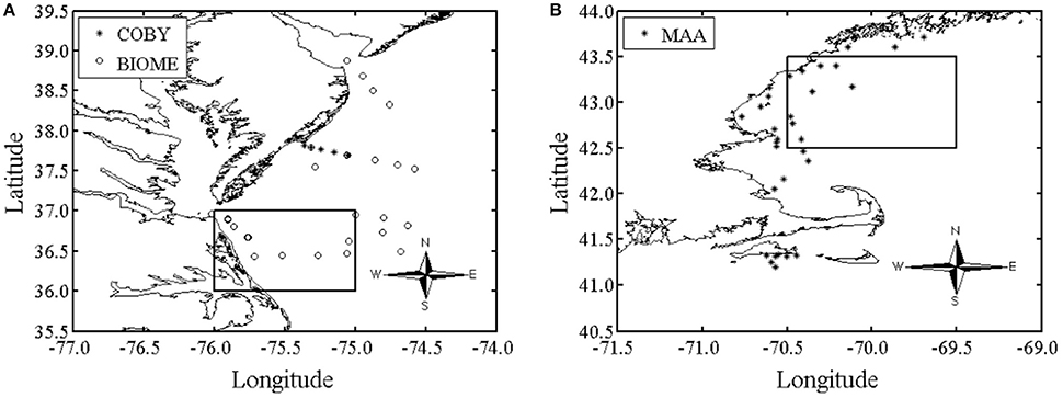
Figure 1. The oceanographic study region was located in: (A) the Delaware, Maryland and Virginia (Delmarva) coastal waters [BIOME and COBY (Bio-physical Interactions in Ocean Margin Ecosystems and Coastal Ocean Buoy Transect), N = 82 samples] during all seasons in 2006 and 2007 and. The square is the area averaged over to represent BIOME in Figure 10. (B) The coastal waters within the Gulf of Maine and near Martha's Vineyard (MAA (Mycosporine-like amino acid), N = 90 samples) during spring of 2007. The data set includes all seasons for the Delmarva region in 2006 and 2007 and only spring samples from the Gulf of Maine in 2007. Both sample regions are along the eastern coast of the United States. The square is the area averaged over to represent MAA in Figure 10.
Phytoplankton Absorption Spectra
Phytoplankton absorption samples were processed using the filter pad technique that partitions absorption into the particulate and detrital fraction (Kishino et al., 1985) to yield a phytoplankton absorption coefficient (m−1; Mitchell, 1990). Absorption spectra were acquired on a Perkin Elmer LS800 UV/VIS Spectrophotometer at 1 nm intervals from 300 to 800 nm using a 4 nm slit-width.
Fluorometric Chlorophyll a
Water samples were filtered with 0.7 μm Whatman GF/F filter (USA), stored in Histoprep tissue capsules, and flash frozen in liquid nitrogen until processing. Chlorophyll a fluorescence was then measured using a Turner Model 10-AU fluorometer (Sunnyvale, USA) according to the method of Welschmeyer (1994). Phytoplankton absorption values were converted to specific absorption (m2 mg chla−1) using fluorometric chlorophyll a measurements. Fluorometric chlorophyll a compared well to ChlHPLC values with an r2 of 0.94.
High-Performance Liquid Chromatography (HPLC) Pigments
Samples were collected from the same Niskin bottles as phytoplankton absorption samples and filtered onto 0.7 μm Whatman GF/F filters. Samples were placed in Histoprep tissue capsules and stored in liquid nitrogen. Phytoplankton pigment concentrations were measured by HPLC on a C18 column using the procedure described by Van Heukelem et al. (2002) at Hornpoint Laboratory. A total of 25 pigment groupings were identified in each of the samples, 18 are calculated in this model, and 8 are used as marker pigments in this study (Table 1). The model pigments are: chlorophyll c, chlorophyllide, phaeophorbide, peridinin, 19′butanoyloxyfucoxanthin, fucoxanthin, neoxanthin, violaxanthin, 19′hexanoyloxyfucoxanthin, diadinoxanthin, alloxanthin, diatoxanthin, zeaxanthin, lutein, chlorophyll b, chlorophyll a, phaeophytin a, and carotenoids (α-carotene, B-carotene, diatoxanthin, diadinoxanthin, alloxanthin, zeaxanthin, lutein, fucoxanthin, peridinin, violoxanthin, 19′butanoyloxyfucoxanthin, and 19′hexanoyloxyfucoxanthin) (Barlow et al., 2007).
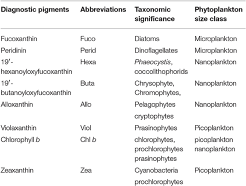
Table 1. Diagnostic pigments used in the present study as biomarkers for phytoplankton functional types (Barlow et al., 1999; Vidussi et al., 2001; Wright and Jeffrey, 2006).
Methods for Modeling Phytoplankton Absorption Spectra and Pigments
Modeled Total Phytoplankton Absorption by Multiple Linear Regression
Total phytoplankton absorption spectra, aph (λ, m−1), was modeled as a second order function of chlorophyll a such that
where Chl a is the concentration of chlorophyll a [mg m−3] and C0, CC, and CC2 are the wavelength-dependent coefficients in the multiple linear regression. The Levenberg-Marquardt non-linear least squares minimization routine (Marquardt, 1963) was used to perform the linear fits using in situ ChlHPLC and aph (λ).
In order to account for pigment packaging effects, the phytoplankton absorption spectra were “normalized” to 675 nm by a normalization term based on the expected unpackaged absorption at 675 nm. The unpackaged or “normalized” absorption spectra is calculated with,
where ci is the concentration of the individual pigments derived from the HPLC analysis and (λ = 675 nm) is the pigment-specific (a.k.a. weight-specific) absorption coefficient at 675 nm for the individual phytoplankton pigments, obtained courtesy of Annick Bricaud (Bricaud et al., 2004).
Modeled Phytoplankton Pigment-Specific Spectra by Matrix Inversion
A goal in modeling phytoplankton absorption spectra, aph(λ) (m−1), is to make use of the reconstruction models to estimate phytoplankton pigments directly from the observed phytoplankton absorption spectra (Moisan et al., 2011). By combining phytoplankton pigment concentrations and pigment-specific absorption spectra, it is possible to reconstruct the total phytoplankton absorption spectra aph (λ) for the sample, such that
where ci (mg pigment m−3) is the concentration of the individual pigments and ai∗(λ) (m2/mg) are phytoplankton pigment-specific absorption coefficients. When a large number (n) of phytoplankton absorption spectra and HPLC observations are available it becomes possible to relate the pigment-specific absorption coefficients and HPLC pigment concentrations to the total phytoplankton absorption measured at a specific wavelength as,
where ci,j is the observed pigment concentration of the ith pigment and the jth sample, (λ) is the derived pigment-specific absorption for the ith pigment, and aph,j(λ) is the total absorption due to phytoplankton for the jth sample and at a given wavelength (λ). At this point the various concentrations and absorption terms are members of a system of linear equations that can be inverted successively using the Singular Value Decomposition (SVD, Press et al., 1987) inversion technique on each wavelength to solve for each of the modeled pigment-specific absorption spectra, (λ).
Pigment Concentrations from Observed and Modeled aph(λ) Spectra
Once estimates for pigment-specific absorption coefficients are available, either through laboratory measurements (Bidigare et al., 1990; Bricaud et al., 2004) or through the numerical inversions such as the SVD approach outlined above, they can be used with phytoplankton total absorption spectra, aph(λ), to estimate the individual pigment concentrations using a second matrix inversion application (Moisan et al., 2011). In this study, we utilized SVD-derived pigment-specific absorption and measured total absorption in the process of estimating phytoplankton pigment concentrations. By expanding the phytoplankton absorption spectra reconstruction technique (Equation 3) of Bidigare et al. (1990) into matrix form, total phytoplankton absorption for a suite of (n) samples can be written as
where (λ) is the estimated pigment-specific absorption of the ith pigment for a given wavelength (λ) obtained from the SVD inversion described in the preceding section, c ai is the estimated concentration of ith pigment for the jth sample, and aph(λ) is the measured total absorption due to phytoplankton at a given wavelength for each j sample.
Phytoplankton pigments were estimated using the resulting pigment-specific absorption spectra obtained from SVD inversion with observed aph(λ). Because solutions to SVD inversions are not guaranteed to produce positive concentrations (negative pigment concentrations have yet to be measured in the ocean), the Non-Negative Least Squares (NNLS, Lawson and Hanson, 1974) inversion method was used to estimate the pigment concentrations to guarantee positive solutions. Moisan et al. (2011) demonstrated that out of all the inversion models tested, SVD-NNLS gave the best results when comparing modeled and measured pigment concentrations. Similarly, this technique has previously been verified in Moisan et al. (2011) through random division of the phytoplankton absorption spectra and pigment measurement pairs. Two independent pools of data were created by randomly separating the full data set in order to carry out the inversions to calculate the pigment-specific absorption spectra and the other to estimate pigment concentrations using the second inversion procedure to validate the model.
In order to apply this matrix inversion technique to satellite data and generate pigment maps, the MODIS Aqua Ocean Color chlorophyll a (ChlSAT) was used with the resulting coefficients from the multiple linear absorption spectra model (Equation 1) to generate predictions of the mapped absorption spectra. These modeled absorption spectra were then inverted, pixel-by-pixel, using the SVD-derived pigment specific absorption spectra from Equation 4 and the NNLS inversion model (Equation 5) to yield maps of pigment concentration for the ocean region of the northeastern United States. Both the linear regression coefficients from Equation 1 and pigment-specific absorption spectra from Equation 4 were obtained using the normalized in situ aph(λ) (Equation 2) and HPLC pigment data. A flowchart of the method summary is detailed in Figure 2.
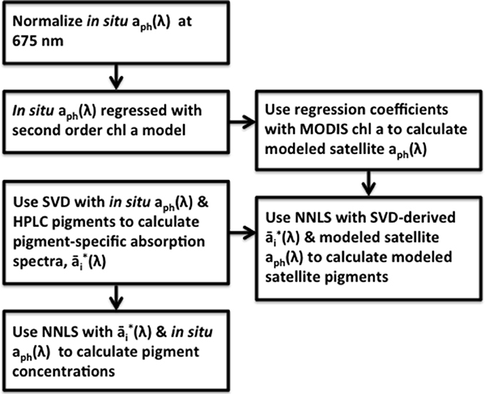
Figure 2. Flow chart of the method utilized in this study to calculate 18 different pigment concentrations along the eastern shore of the United States. The linear absorption spectra model developed in Moisan et al. (2013) is modified and used with the matrix inversion techniques developed in Moisan et al. (2011) in order to extend the matrix inversion technique for use with satellite data.
The matrix inversion technique applied to satellite data uses modeled instead of in situ absorption. In order to assess how the pigment inversions are affected by the use of modeled absorption, the results from the inversion model using modeled versus measured absorption spectra is compared.
Phytoplankton Functional Type Maps and Diversity
Once maps of the various 18 phytoplankton pigments were obtained, they were used to generate estimates of the various PFTs for the region by using the estimation formulas outlined in Table 1 of Hirata et al. (2011) for diatoms, dinoflagellates, prymnesiophytes, prokaryotes, and green algae (Table 2). The pigments necessary as inputs for these algorithms included: fucoxanthin, peridinin, chlorophyll-b, 19-butanoyloxyfucoxanthin, 19-hexanoyloxyfucoxanthin, alloxanthin, and zeaxanthin. Maps of these functional types were calculated for all of the MODIS Aqua data used in this study domain and period.
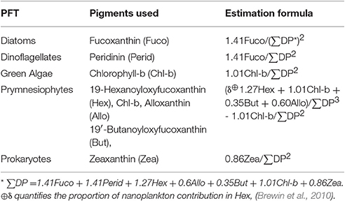
Table 2. Phytoplankton Functional Type (PFT) equations (Hirata et al., 2011) used in this study.
After calculation of the PFT fields, the PFTs Diversity was calculated using the Shannon Diversity Index (H) equation,
where pi is the ith proportionality of the N phytoplankton functional groups (Shannon, 1948). Proportionality values, pi, were defined as the resulting PFT values, the ratio of chlorophyll for that functional type versus the total chlorophyll within a sample. While the Shannon Diversity equation was developed to use specific cell or organism counts, a sensitivity study was conducted that used randomly chosen cell to biomass ratios in order to see what the impact of this had on the resulting H values, assuming that the conversion factors were constant throughout the study's time and space domain. The results showed little impact on the resulting H values meaning that the method used in calculation of the proportionality values was justified.
Results
Observations of Absorption Spectra
Values of aph(λ) showed large variability in the ultraviolet (UV) and visible region (Figure 3). UV absorption was high, presumably due to mycosporine-like amino acids (MAAs, Moisan and Mitchell, 2001) and was commensurate with a Phaeocystis-dominated community in the Gulf of Maine. MAA absorption peaked at the surface of the ocean and is most likely controlled by irradiance and nutrient concentration (Whitehead and Vernet, 2000). Phytoplankton maximum absorption in the UV region ranged from 0.28 to 0.85 m−1. Maximum values of aph(λ) in the visible ranged from 0.03 to 0.37 m−1 (Figure 3). Values of aph(436:676), the red and blue absorption peaks of chlorophyll a, varied by an order of magnitude, with highest levels associated with elevated levels of carotenoids, indicating growth in a high-light environment. Minimum and maximum values for aph(436:676) are 0.006 and 0.369 and 0.003 and 0.198, respectively.
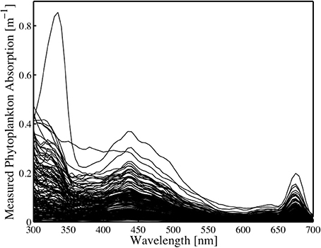
Figure 3. In situ phytoplankton absorption (m−1) from samples collected during the study.
Modeling of the Total Absorption Spectra
In order to model the absorption spectra, the spectrally-dependent, linear model coefficients from Equation 1 were used with ChlHPLC values. The r2 values of in situ versus modeled absorption, when normalized to 675 nm, are between 0.76 and 1.00 from 400 to 700 nm and drop by about 25%, as calculated by dividing the mean r2 of UV and visible groups, in the ultraviolet region (Figure 4) where MAAs provide sun screening to phytoplankton and increase the observed value of aph(λ). Accuracies were substantially improved using the “normalized” absorption spectra in Equation 1, compared to original in vivo absorption spectra (Moisan et al., 2011).
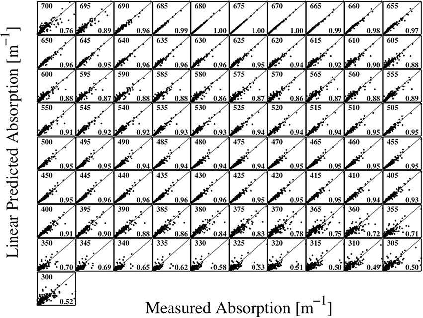
Figure 4. Measured total absorption (m−1) normalized to 675 nm (horizontal axis) versus the predicted total absorption (m−1) (vertical axis) using the multiple linear regression of ChlHPLC and ChlHPLC2.
To assess how much of the variability in the absorption curve is accounted for in the absorption model, the root mean square error (RMSE) was calculated for the first, second, and third order absorption models. The RMSE is the square root of the mean of the square of all the error. The variance drops by half from the observed spectra to the first order modeled spectra (RMSE = 0.113 and 0.063, respectively), and only slightly decreases with the second and third orders (RMSE = 0.063 and 0.060, respectively). Beyond the first order regression model there are only small improvements in modeling the absorption spectra. However, while the second order model is only slightly better than the first order in representing the variability of the absorption spectra, a larger improvement is observed in the pigment retrieval solutions. This may be because small improvements in modeling the absorption spectra can have a significant impact on the solution of those pigments that have smaller contributions to the total absorption spectra. The second order ChlHPLC model was chosen because there are only marginal difference between first, second, and third order in modeling absorption and second order produces the best pigments retrievals.
Observations of Pigments in Relation to Absorption Spectra
The contribution of each of the 18 pigments estimated by the inverse model to total absorption was determined by reconstructing the absorption spectra following the technique developed by Bidigare et al. (1990) and utilizing the pigment-specific absorption coefficients from Bricaud et al. (2004) and the in situ HPLC pigment measurements (Figure 5A). The standard deviation of these individual absorption spectra (not shown) scale directly with the standard deviation of the various pigments observed, which is considerable. An analysis of the individual pigment contributions to the total absorption spectra, shown as a cumulative function, demonstrated that ChlHPLC, fucoxanthin, chlorophyll c, diadinoxanthin and carotenoids together account for more than 90% of the observed in vivo absorption (Figure 5B). Coincidentally, these pigments were shown to have the highest predictive capability for the SVD-NNLS model that yields pigment-specific absorption spectra and HPLC pigment estimates (Figure 5B). Those pigments that contributed significantly to aph(λ) and account for the majority the absorption were also those that were best predicted using the SVD-NNLS inversion model.
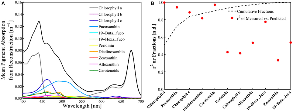
Figure 5. (A) Reconstructed mean pigment-specific total absorption spectra (m−1) of the different pigment biomarkers resolved in this study. The black line is the total absorption of all pigments. The lowest standard deviation values were insignificant, while higher standard deviation values for the pigments ranged from 0.0015 to 0.0686. (B) Cumulative fraction of the reconstructed pigment absorption to total absorption compared to the r2 from the inverse model versus predicted HPLC pigments from SVD-NNLS.
Individual Photosynthetic and Photo-Protective Pigment Retrievals
Pigments were estimated by the NNLS matrix inversion (Equation 5) with the SVD-derived pigment-specific absorption from Equation 4 and in situ absorption spectra. A comparison of in situ measured to SVD-NNLS-derived HPLC pigments shows varying results with coefficients of determination ranging from very high (near 1.0) for chlorophyll a () to a low of 0.33 for zeaxanthin (Figure 6). While 18 different pigments were estimated, only 10 had r2 values greater than 0.68. The p-values of the algorithm were calculated with a threshold value of 0.05. All pigments had p-values of less than 0.001, demonstrating that the results are significant (Table 3). Similarly, the pigment concentrations on a normal scale produced relatively small RMSE for most pigments, with normalized RMSE less than 22% for all pigments, except zeaxanthin and lutein. Normalized RMSE is the RMSE divided by the pigment range and bias is the tendency of a statistic to overestimate or underestimate a parameter. Pigments that correlate best with ChlHPLC, such as chlorophyll c, fucoxanthin, and carotenoids, along with ChlHPLC account for the majority of the total absorption spectra (Figure 5B). These pigments are also shown to have the best prediction results when modeled pigment concentrations are compared with in situ concentrations: they have the highest r2 values, their slopes are very close to 1 with y-intercepts close to 0, normalized RMSE below 5%, and all have p-values below the 0.05 threshold. While the coefficients of determination for the predicted pigments vary, all are within the acceptable range of algorithms that predict PFTs (Hirata et al., 2008, 2011; Bracher et al., 2009; Mouw and Yoder, 2010; Mouw et al., 2012; Soppa et al., 2014). In addition, even with the known uncertainties, the resulting maps of PFTs can be useful for phenological functional diversity studies.
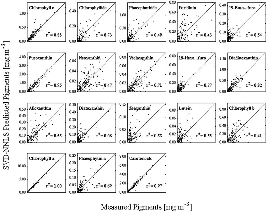
Figure 6. HPLC measured pigments (horizontal axis) versus the predicted pigments (vertical axis) using SVD to obtain the pigment-specific absorption spectra and NNLS to obtain pigment estimates.
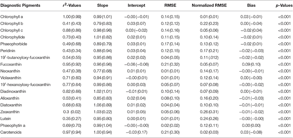
Table 3. Statistical values derived from comparison of measured pigment concentrations with those estimated from the SVD-NNLS inversions using the measured (modeled) absorption spectra.
Applying Inversion Model to Satellite Data
Modeling phytoplankton absorption spectra at every 5 nm using satellite chlorophyll a observations allows for extrapolation of observed relationships and can account for changes due to spectral shape, pigment composition, and pigment packaging (Figure 4). To apply the inversion model to satellite data, we calculated absorption (Equation 1) and inverted the modeled absorption values to obtain estimates for 18 HPLC pigments over a series of remote sensing images of the northeastern US coastal ocean. To demonstrate that the modeled absorption (as opposed to in situ absorption) would not have a significant effect on the pigment retrievals, we ran the SVD-NNLS inversion model using HPLC pigments and absorption modeled from Equation 1 and compared the resulting modeled pigment concentrations with in situ concentrations. While the r2 values in general decreased and the normalized RMSEs increased, compared to the inversion with in situ absorption, the r2 values of the predicted pigments that are addressed in detail in the analysis were not significantly less (Table 2). The statistical comparison of the two methods demonstrated that using modeled absorption in the satellite inversions does not significantly impact the pigment retrievals.
The results from the satellite-based inversion model show that the resulting estimates of chlorophyll a () maps are similar to those from the standard MODIS Aqua ChlSAT product (data not shown). A linear comparison of ChlSAT and ChlSAT results in an r2 of 1.00. While the OC-4 algorithm, applied to any of the NASA ocean color satellites (SeaWiFS, MODIS Terra and Aqua) has known issues with predicting chlorophyll a in coastal regions, the results from this study demonstrate that on a larger regional scale the features for both the OC-4 algorithm and the SVD-NNLS model solutions have very similar spatial scales and features.
To quantify the inherent error of using ChlSAT in the inversion model, we gradually introduced normal random error ranging from zero to a level comparable to the MODIS Aqua ChlSAT (r2 ~0.75) into the ChlHPLC and ran it through the SVD-NNLS inversion model. After hundreds of iterations, our mean r2 values for pigment retrieval dropped by 15–30 percent when errors were compatible to the satellite error which implied that the introduction of the satellite error does not greatly diminish the results of the inversion analysis (Figure 7).
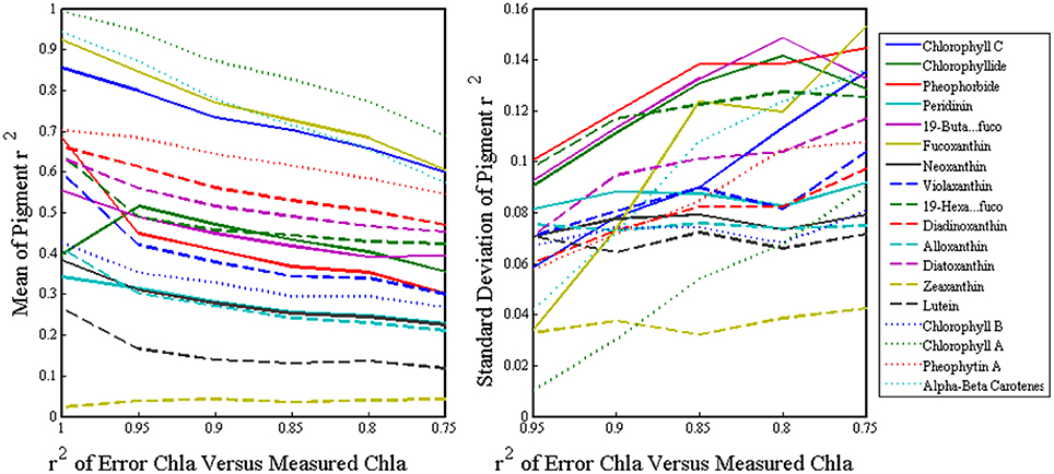
Figure 7. The x-axes are the r2 of the ChlHPLC versus the ChlHPLC with normal random error added, where 1 is ChlHPLC with no error and 0.75 is equivalent to the error of ChlSAT. The y-axes depict the mean (left) and standard deviation (right) of the r2 values of the measured versus predicted pigment concentrations after the inversions are run with errored ChlHPLC for hundred of iterations.
In addition to , inversion of absorption spectra over a larger regional domain yielded estimates of 18 photosynthetic and photo-protective pigments for the year 2007 (Table 2). A number of these are useful as biomarkers for certain PFTs and can aid in resolving phytoplankton community structure (Table 1). Maps of pigments normalized to biomass (using ) are markers for the distribution of PFTs within a region (Figure 8).
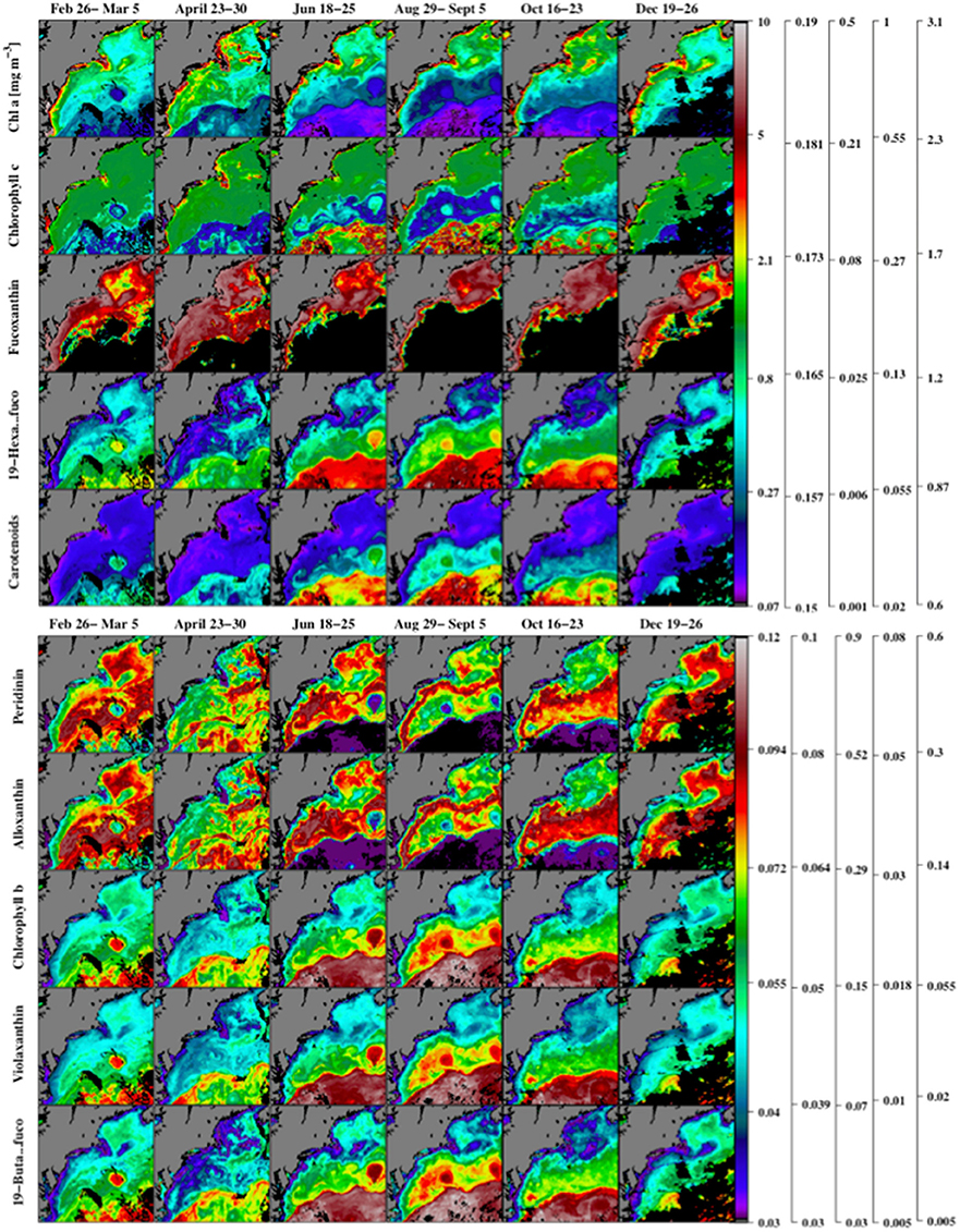
Figure 8. Maps of the satellite-based inversion model estimates of chlorophyll a, and the ratios of chlorophyll c, fucoxanthin, 19′hexanoyloxyfucoxanthin, carotenoids (α-carotene, B-carotene, diatoxanthin, diadinoxanthin, alloxanthin, zeaxanthin, lutein, fucoxanthin, peridinin, violoxanthin, 19′butanoyloxyfucoxanthin, and 19′hexanoyloxyfucoxanthin) to (upper panel) using MODIS Aqua 2007 chlorophyll a observations. Similar ratios of peridinin, alloxanthin, chlorophyll b, violaxanthin, and 19′butanoyloxyfucoxanthin to are shown in the lower panel. Note that the nonlinear colored scale bars differ for each pigment, and the scales from left to right are associated with the pigments from top to bottom. Regions where the inverse model yielded zero concentrations are shown in black.
Chlorophyll a Distribution
Modeled distribution from the SVD-NNLS inversion process compares well with MODIS Aqua ChlSAT distribution with r2 value of 1.00, and they both were inversely correlated to observed MODIS Aqua SST (data not shown), with highest (coldest) levels of ChlSAT (SST) located along the coast and over the well tidally-mixed region of the Grand Banks, with lowest (warmest) levels offshore to the southeast near the Gulf Stream Province, as noted by Longhurst (2010). However, while the inverse model solutions compare well with the satellite observations, the technique does not eliminate the inaccuracies inherent in using satellite observations. A recent study comparing in situ chlorophyll a measurements and MODIS-Aqua chlorophyll a OC3 retrievals (Kahru et al., 2014) shows that the coefficient of determination (R2) values were 0.86 for all measurements but that R2 dropped to 0.35 for comparisons matchups with chlorophyll levels > 1.0 mg Chla m−3. In addition, an earlier work by Thomas et al. (2003) focusing on the region of the Gulf of Maine (a subdomain of our study) notes that summertime matchups of log-transformed in situ chlorophyll to SeaWiFS chlorophyll have an r2 of 0.55. Most of the errors in these estimates seem to be limited to the higher chlorophyll regions (>1.0 mg m-3) regions along the coast, which were only a small part of the overall study domain. For the most part, MODIS-Aqua underestimates the higher chlorophyll a levels observed in the coastal region and underestimates the lower chlorophyll a values found in the offshore region, thereby reducing the overall gradients in the true chlorophyll a fields. Such a cross-domain bias serves only to distort the resulting pigment retrievals by diminishing the gradients, while keeping distinguishable the larger scale pigment patterns and time series variability.
Phytoplankton Functional Type Marker Pigment Distributions
Identification of the presence of specific PFTs using marker pigments has been shown to be possible for a number of functional types (Wright, 2005). Although most pigments are not unique to specific phytoplankton taxa, and only a limited number are unambiguous pigments for specific phytoplankton taxa (Nair et al., 2008), it is possible to make valid inferences using in situ field measurements for verification of functional type distributions.
Maps of several key PFT marker pigments, normalized to chlorophyll a, obtained from the inverse model (Figure 8) solutions for 2007 show a range of different spatial distributions over the study region. A small group of pigments (notably chlorophyll a, and fucoxanthin) show a strong spatial correlation with chlorophyll levels, and are highest in the coastal regions and lowest offshore. Fucoxanthin is primarily a marker pigment for diatoms, though it is also associated with other phytoplankton types and therefore has been argued to be ambiguous as a marker pigment (Nair et al., 2008). A second group of marker pigments (peridinin and alloxanthin) shows highest pigment to chlorophyll a ratios in the mid-shelf region of the study area. Peridinin is a marker pigment for Type-I dinoflagellates (Ornótfsdóttir et al., 2003) and alloxanthin is a marker pigment for Cryptophytes (Wright, 2005). A third larger grouping of marker pigments (19′hexanoyloxyfucoxanthin, chlorophyll-b, violaxanthan, and 19′butanoyloxyfucoxanthin) and carotenoids show highest pigment to chlorophyll levels in the offshore region of the study area. All of these pigments are ambiguous marker pigments, but have been used in prior studies to infer distributions of haptophytes (Mackey et al., 1996).
Spatial Distribution and Phenology of Phytoplankton Marker Pigments
The seasonality of the functional type marker pigments (Figure 8) co-varied strongly with phytoplankton biomass levels, estimated by chlorophyll a concentrations, even though the ratios of the marker pigment concentrations to biomass levels varied spatially over the study region. Three specific regions related to the MAA sample area (coastal Gulf of Maine), the BIOME sample area (coastal region of the mid-Atlantic Bight), and for an open ocean region near the southeast associated with the Gulf Stream Extension domain were chosen as representative study regions (not shown). MODIST Aqua from 2002 to 2016 was taken for these three square areas and run through the inversion method to calculate 18 pigment concentrations that were averaged over each region. The spatially-averaged time series of the phenologically related marker pigments within each of the three regions from 2002 to 2016 (not shown) demonstrates that these key pigments vary differently from region to region.
levels for all regions showed seasonal variability, but no similarities (Figure 8). A review of the variability in this region is given by O'Reilly and Zetlin (1998). The BIOME region showed peaks in during its noted wintertime-spring bloom that is associated with the well-mixed water column. The open ocean region shows bloom levels of rising more than two fold, with a larger peak bloom occurring in the spring followed by a less dramatic bloom in the fall. The coastal Gulf of Maine (MAA) region shows late spring blooms marked by lowest levels in mid-winter.
Fucoxanthin to ratios, a marker pigment for diatoms, showed high variance and an inverse correlated with SST over the time series (2002–2016) analyzed. The open ocean region showed the highest variance and a bi-annual peak in ratios in the spring and fall, possibly due to spring and fall diatom blooms. The BIOME region (northern coastal) showed high, low variance and nearly constant ratios during the fall through winter period, with a decrease during the summer seasons only. Finally, the MAA (southern coastal) had the highest observed variability, which, like the BIOME region, showed large decreases, but timed to occur primarily during the winter periods.
The 19′hexanoyloxyfucoxanthin to ratios (prymnesiophytes, Phaeocystis pouchetii and coccolithophorids) covaried with SST, with peak levels observed in the open ocean during the summer months, followed by the BIOME, with lowest peaks at the MAA site.
Peridinin: ratios (dinoflagellates) on the other hand showed an inverse correlation with SST except in the Biome region, peaking in concentration in the winter months when temperatures were at their lowest and mixed layer depths were at their greatest. Like the phenology of the 19′hexanoyloxyfucoxanthin-related PFTs, peridinin showed highest ratios in the open ocean site. However, higher peaks in the ratios were observed for the MAA region with lower levels in the BIOME region, noting that the dinoflagellates preferred more northerly coastal regions.
Phytoplankton Functional Type Distributions, Phenology, and Diversity
Maps of five PFTs (diatoms, dinoflagellates, prymnesiophytes, prokaryotes, and green algae) calculated using the equations developed by Hirata et al. (2011; Table 1) were generated using the resulting pigment maps obtained from the inverse model using the MODIS-Aqua chlorophyll observations from the study region.
Diatom Distributions
Diatom distribution was assessed by utilizing fucoxanthin as its biomarker pigment. Fucoxanthin is a useful marker for the bacillariophyceae or diatoms (Table 1) and also occurs in the raphidophytes and some prymnesiophytes (Jeffrey and Vest, 1997). Quantile regression analysis of HPLC fucoxanthin relative to 19′hexanoloxyfucoxanthin observations, as carried out in Devred et al. (2011), revealed slightly elevated concentrations of fucoxanthin relative to 19′hexanoloxyfucoxanthin, indicating a negligible contribution of fucoxanthin to prymnesiophytes. After the calculation of microplankton and nanoplankton percentages from pigment concentrations, fucoxanthin on average accounts for about 20% of nanophytoplankton and 80% of microphytoplankton (data not shown, Devred et al., 2011). The diatom's marker pigment, fucoxanthin, had a high correlation coefficient (r2 = 0.95) between in situ and modeled values (Table 2). Other accessory pigments found in diatoms, such as chlorophyll c and photo-protective pigments, had average r2 values of ~0.97. The observations show that diatoms were taxonomically dominant throughout the year (Figure 9), with fall and spring peaks in their biomass as shown in the chlorophyll a observations (Figure 8). This has been shown previously in this region using radiance measurements to estimate PFTs (Pan et al., 2010). Diatoms were the dominant coastal region functional type, accounting for well over half of the phytoplankton biomass, relative to chlorophyll a levels. The time series of the diatom populations averaged over three separate regional areas in the study site (Figure 10) and the climatology between 2006 and 2011, shows that the diatom population has highest concentrations in the coastal Gulf of Maine (Figure 1B, MAA) region, with a slight decrease during the summer stratified season. High levels are also observed in the coastal Delmarva region (Figure 1A, BIOME), but with two nearly similar peaks, one in the spring and the other in the fall. The open ocean region (not shown, site domain is 69°–68° west longitude and 38°–39° north latitude) diatom levels are lowest of the entire domain but exhibit relatively strong spring and modest late fall blooms. For much of the summer periods in the open ocean region, chlorophyll levels are below the ~0.45 mg chla m−3 cutoff levels, below which fucoxanthin pigments are not retrieved in the inverse model solutions. For those periods of time the diatom levels are estimated to be minimal or irrelevant relative to the rest of the PFT population.
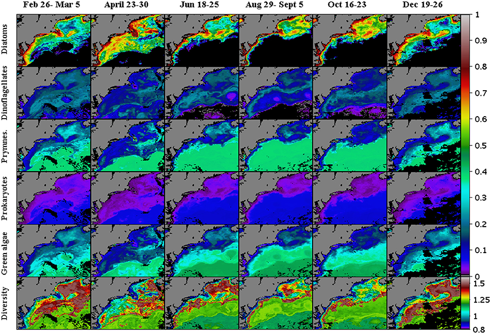
Figure 9. Modeled weekly-mean phytoplankton functional types and calculated Shannon Diversity Index during 2007. Starting from the upper row of images are distribution maps of Diatoms, Dinoflagellates, Prymnesiophytes, Prokaryotes, and Green Algae (% chlorophyll a). Weekly maps of the Shannon Index (H; n.d.) for the PFT diversity are shown along the lower row of panels. Regions where the inverse model yielded zero concentrations are shown in black.
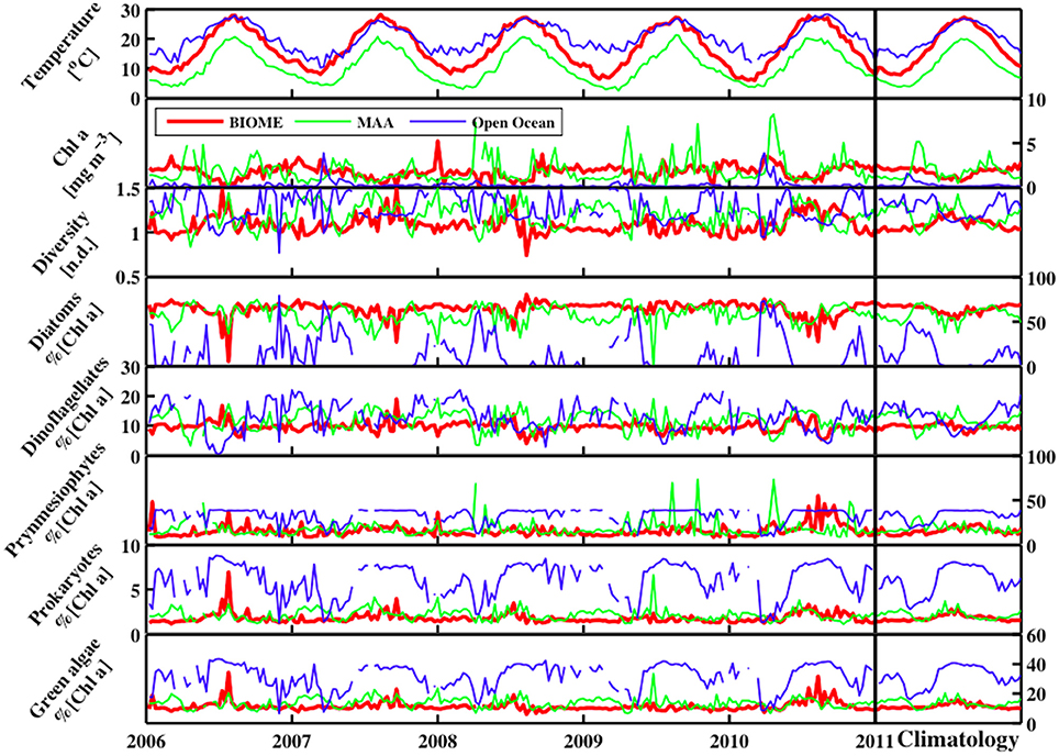
Figure 10. The temporal distribution for sea surface temperature (°C), ChlSAT, Shannon Diversity Index (H; n.d.), and phytoplankton functional types (% chlorophyll a) for Diatoms, Dinoflagellates, Prymnesiophytes, Prokaryotes, and Green Algae from 2006 to 2011 for three stations including the Mid Atlantic Bight, Gulf of Maine, and open ocean.
Within the study region, diatoms played a dominant role in shaping the diversity in areas with chlorophyll levels greater than 0.45 mg chla m−3 (Figure 11). A peak of ~1.5 in diversity levels is observed at chlorophyll levels of ~0.82 mg chla m−3 which is driven entirely by the rise in contribution in total biomass from the diatom fraction of the PFTs. Below the 0.45 mg chla m−3, diatoms play little to no role in determining the functional type diversity levels.
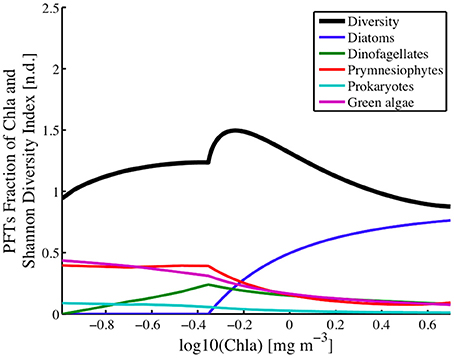
Figure 11. Phytoplankton functional types (fraction of chlorophyll a) for Diatoms, Dinoflagellates, Prymnesiophytes, Prokaryotes, and Green Algae, and Shannon Diversity Index (H; n.d.) plotted against the log of ChlSAT over the whole study region.
Dinoflagellate Distributions
Peridinin was the biomarker pigment used to calculate the distribution of dinoflagellates (Table 1) according to Hirata et al. (2011; Table 1). Concentrations of both measured and modeled peridinin were generally less than 0.8 mg peridinin m−3, with a modest 0.49 r2 (Figure 6) in the one-to-one comparisons. In terms of its importance to total absorption reconstruction, it ranks sixth. Maps of the modeled pigment to chlorophyll a ratios of peridinin were low and ranged from 0.00 to 0.12 (mg peridinin/mg chla, (Figure 8). Maps of the dinoflagellate populations show that they were present in highest concentrations in the mid-shelf regions of the study site (Figure 9), being at their highest concentrations in the winter months for the MAA and open ocean regions but at lower and less variable levels in the BIOME domain where no seasonal variability was observable. Lowest levels of dinoflagellates were estimated to be present in the late spring for the MAA region and in the mid-summer for the BIOME region. Late summer maximum levels retreated to a region running along the shelf front along the outer region of the Gulf of Maine and south along the coast (Figure 9).
Unlike the diatom populations, dinoflagellates influence diversity across all levels of biomass. Their peak influence in diversity occurs at chlorophyll levels of 0.45 mg chla m−3, which is where the diatom populations, or more correctly where fucoxanthin estimates go to zero. At lower phytoplankton biomass, or chlorophyll levels below the peak, the contribution of dinoflagellates to phytoplankton functional diversity levels decreases to zero at chlorophyll a concentrations of 0.1 mg chla m−3. At higher phytoplankton biomass or chlorophyll levels above the peak, the contribution of dinoflagellates to PFT diversity also decreases but at a much slower rate, reaching a near constant level at the higher chlorophyll levels.
Green Algae
Green algae is a large, diverse and informal group, in the planktonic ocean realm this group is composed primarily of chlorophytes (Prasinophyceae (i.e. Ostreococcus), micromonas). The distribution of this PFT's taxonomic importance closely resembles that of the Prokaryotes and Prymnesiophytes. Concentrations of green algae were estimated according to Hirata et al. (2011; Table 1) using estimates of chlorophyll-b concentrations. Maps of the green algae distribution (Figure 9) show that the green algae were the dominant PFT in the open ocean, where they accounted for nearly 40% of the phytoplankton biomass (Figures 10, 12). In this offshore domain, large spring and smaller fall diatom blooms correlated with a decrease in the green algae levels during those periods. Green algae contributions to the PFT diversity was highest (~38%) in the open ocean, low chlorophyll a domain and remained relatively constant with increasing chlorophyll a levels until it encountered the transition region where the diatom population begins to appear in the solutions. For chlorophyll levels above 0.45 mg chla m−3, the green algae biomass (Figure 11) and their contributions to the PFT diversity continued to decline with increasing levels of chlorophyll a.
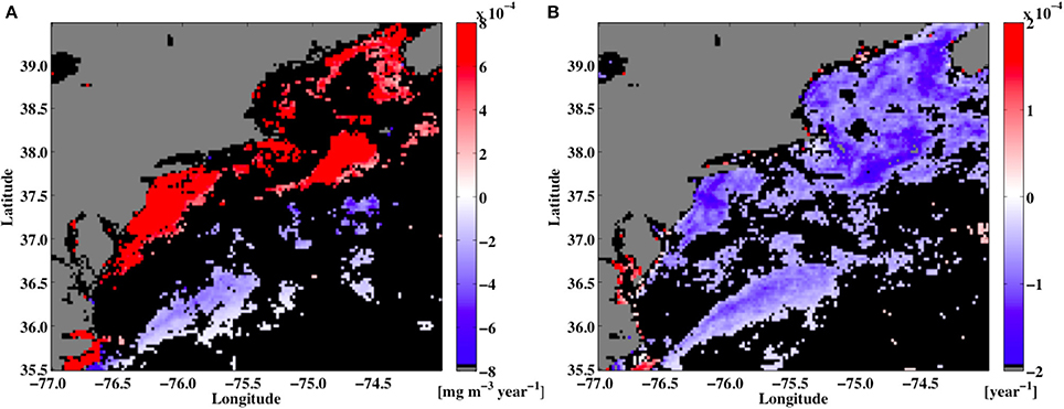
Figure 12. The trend line slopes of (A) seatellite chlorophyll a [mg chla m−3 year−1] and (B) shannon Diversity Index [H; year−1] at each point over a 15-year period (2002–2016) in the study region. Regions where the slopes were insignificant are shown in black.
Prymnesiophyte (Haptophyte) Distributions
Concentrations of haptophytes were estimated according to Hirata et al. (2011; Table 1) using estimates of 19′hexanoyloxyfucoxanthin and 19′butanoyloxyfucoxanthin concentrations to estimate total nanoplankton from which the estimates of green algae are subtracted. While 19′hexanoyloxyfucoxanthin is an ambiguous marker pigment for functional types, it is associated with prymnesiophytes, i.e., Phaeocystis pouchetii, and coccolithophorids (Table 1). Both Phaeocystis sp. and the diatom Skeletonema costatum dominated the bloom in the Gulf of Maine during April, 2007, where a mesoscale bloom was persistent during the spring (Figure 8). The results show that when diatom blooms occur the importance of Prymnesiophytes within the phytoplankton population declines relative to the diatom levels both in terms of concentrations (Figure 10) and their contribution to the diversity levels (Figure 11). Prymnesiophytes generally were found to be higher in the offshore ocean regions and diminished onshore relative to the per unit chlorophyll levels in each region. Seasonally, Prymnesiophytes showed broadly varying seasonal cycles in the BIOME and MAA regions, with peaks in percent chlorophyll levels occurring in late summer. The open ocean levels were predominantly flat except when the spring diatom bloom appeared.
Prymnesiophytes influence the PFT diversity levels (Figure 11) only at chlorophyll levels greater than 0.45 mg chla m−3, with highest influence at this transition chlorophyll concentration and a minimal impact at chlorophyll levels of ~3.2 mg chla m−3. Below 0.45 mg chla m−3, its contribution to the PFT diversity is equal to that of the green algae and constant at around 35%. Prymnesiophytes and the green algae showed strong correlations in terms of their spatial distribution and their contribution to PFT diversity as a function of chlorophyll a levels.
Prokaryotes
Maps of the prokaryotes (cyanobacteria) show distributional patterns that correlate strongly with the patterns observed in the green algae and Prymnesiophyte distributions. Estimates of the distribution of this group shows that they are more taxonomically important in the warmer, more stratified region of the study domain, and highest concentrations in the southeastern region where low nutrient gulf stream waters are found. In terms of percent chlorophyll, the Prokaryotes accounted for the lowest percentage of total biomass, with the highest percentages found in the offshore southeastern domain with values near 5%, and diminishing to near 2% for both the MAA and BIOME regions. During the warmer season, when nutrients are lower and stratification is high they have been observed to thrive in the coastal regions that have highly stratified water, such as the coastal areas off the Delmarva Peninsula region (Moisan et al., 2010). The seasonal cycles of both the MAA and BIOME regions showed modest peaks in the winter and summer time periods. Overall, prokaryote distributions over time were similar to that of the prymnesiophytes and green algae, and they varied inversely with the concentrations in diatom populations.
Phytoplankton Functional Type Diversity
Maps of the PFT diversity (Figure 9), calculated using the Shannon Diversity Index (H, Equation 6) and PTF proportionality values of the various five (diatoms, dinoflagellates, prymnesiophytes, prokaryotes, and green algae), show that a dynamic field of PFT diversity exists in the study domain. Highest levels of diversity are seen between the nearshore high chlorophyll regions and the offshore oligatrophic regions, with the most extensive areas showing up during the winter and spring time and having lowest extent in the summer when the region is isolated to the Gulf of Maine and along the coastal shelf region along the entire study domain.
Because of the methods used to generate PFT estimates, the suites of phytoplankton pigment estimates, the PFT concentrations, and the Shannon Diversity Index (H) are all non-linear functions of chlorophyll a concentrations (Figure 11). The results show that the majority of the PFT concentrations or relative abundances vary smoothly across chlorophyll levels ranging from 0.01 to 10.0 mg chla m−3. A peak in the diversity is seen at chlorophyll levels of 0.63 mg chla m−3, with diversity levels decreasing at lower and higher concentrations of chlorophyll a. The peak itself is part of a localized higher (>0.8) diversity estimate for chlorophyll levels ranging between ~0.45 and ~1.0 mg chla m−3. This high PFT diversity region is located along the shelf at all times of the year and within the majority of the Gulf of Maine except along the near coastal areas. The overall area of high diversity expands to larger open ocean areas in the winter (Figure 9), when diatom levels are lower and become closer to the concentrations of the green algae, dinoflagellates and prymnesiophytes.
The local time series dynamics of both the PFTs and the resulting H show a wide range of variability (Figure 10). Overall, along the southern coastal BIOME region, the climatology in H shows a smooth seasonally varying relationship with a maximum level of diversity in the summer season. In the coastal Gulf of Maine MAA domain, the seasonal cycle in the H values shows high levels in the winter and summer season, with lows in the spring and fall due to the diatom bloom. In both the MAA and BIOME regions, increases in H are directly correlated with decreases in chlorophyll a or phytoplankton biomass. In the open ocean, chlorophyll a levels fluctuate around the peak in the H versus chlorophyll a relationship (Figure 11), leading to a much more variable climatology in H for this region. For instance, during the start of the spring bloom period in the open ocean domain, when the diatom population begin blooms and the winter population of prymnesiophytes, prokaryotes, and green algae are in decline, H increases until the chlorophyll a levels pass beyond the 0.63 mg chla m−3 level, above which H levels drop as the diatom population continues to bloom. This peak in the H versus phytoplankton biomass or chlorophyll a levels creates a much more complex H climatology for areas of the domain where the mean chlorophyll a levels are at this peak in H. Surprisingly enough, this chlorophyll a level is very near the peak in the histogram (not shown) of the chlorophyll a values for the domain. The belief is that this is merely serendipity from the choice in the domain under study, and not an ecological observation.
In addition to the complexities arising from the non-linear relationship between chlorophyll a levels and PFT diversity, the impact of climate-scale changes in the chlorophyll a field can also result in changes in PFT H values. For instance, for the 3 × 3 pixel region of the MODIS Aqua data centered on the location of the Woods Hole Oceanographic Institution's Air-Sea Interaction Tower (ASIT; 41° 19.5′ N, 70° 34.0′ W), the PFT diversity time series (not shown) has a seasonal cycle and a significant (p-value was 0.028) negative trend in the overall PFT diversity for that location. This trend is due to changes in the chlorophyll a levels during that period of time.
Maps of chlorophyll a linear trends for the study domain (not shown) reveal that the coastal ocean areas have positive trends in chlorophyll levels but negative trends are seen in the open ocean regions. The majority of the domain (~70%) shows no significant trends in the chlorophyll a levels. So for the study domain, some areas have observed rising chlorophyll a levels (along the coast) and in other regions chlorophyll a levels fall (open ocean). However, because the relationship between chlorophyll a levels and PFT diversity is non-linear, the long-term trends in PFTs can also vary. So, while the resulting trends in the chlorophyll maps for the region showed some areas of positive and negative trends, the trends for the PFT H values were nearly all negative.
Discussion
The aim of this study is to demonstrate how a technique that uses both an inverse model (Moisan et al., 2011) and a pigment-dependent algorithm (Hirata et al., 2011) to predict phytoplankton biodiversity can be used to estimate PFT diversity over a much larger area than was sampled, while maintaining robust results that retain the unique spatial and temporal features of the MODIS-Aqua ChlSAT data. The key to retaining original features of the chlorophyll a data is the second order chlorophyll a model and matrix inversion model that convert ChlSAT into phytoplankton absorption from 300 to 700 nm at a high resolution of 5 nm which is then converted into 18 different marker pigments (Moisan et al., 2011, 2013). Using total absorption spectra derived for a variety of coastal and open ocean environments, the algorithm was able to predict phytoplankton absorption and pigments in Longhurst (2010) provinces including the Gulf Stream Province, N. Atlantic Subtropical Gyral Province, and the NW Atlantic Shelves Province. Interestingly, the phytoplankton community did not necessarily follow Longhurst's provinces, but is divided into a delineated coastal community, offshore community, and one that moves offshore and onshore with the seasons. The results have implications for understanding how different phytoplankton groups compete with each other in different biological provinces within the ocean.
The accuracy in terms of r2 of the pigments predictions from inverting absorption spectra are highest when in situ data are used (Table 2). The accuracies increase when regressing absorption spectra with an additional pigment packaging parameter (O'Reilly and Zetlin, 1998; Alvain et al., 2005). An increase in the accuracy of the predicted phytoplankton absorption and pigments was retrieved when pigment package effects were parameterized (Johnsen et al., 1994; Bricaud et al., 1995; Ciotti et al., 2002) by “normalization” of the measured absorption spectra to the expected absorption at 675 nm. The spectral shape of the pigment package effect shows modest variability across the spectrum (Morel and Bricaud, 1981). Inaccuracies are factored into the equation when pigment package effects are taken into account. Also, Bricaud et al. (2004) claims that a term is missing when reconstructing the in vivo absorption spectrum of natural populations from pigment concentrations. Another factor that introduces error into the pigment estimates are the linear regression technique that has a fair r2 value of 0.76 to 1.0 of modeled to in situ absorption from 400 to 700 nm. The matrix inversion method produced estimates of marker pigments that compared well against the measured HPLC pigment observations, with r2 values averaging 0.70. The technique was robust for all pigments except zeaxanthin and lutein (Figure 6). The resulting range of r2 values obtained in this study (r2 0.33–1.0) are similar to those obtained by Pan et al. (2010) from a related study that estimated pigment concentrations (r2 0.4–0.8) using in-water radiometry measurements off the northeast U.S. continental shelf. The satellite data driven aph(λ) model accurately captured the variability with respect to its shape and magnitude caused by pigment concentrations, variable pigment ratios, and pigment packaging (Moisan and Mitchell, 1999).
The techniques's use of pigments estimates with algorithms for PFTs should be used with caution because pigment ratios can vary with phytoplankton species composition, light history, and acclimation to temperature and nutrients (Moisan and Mitchell, 1999; Louanchi and Najjar, 2001; Woodward and Rees, 2001; McGillicuddy et al., 2003; Geider et al., 2014). In this paper, PFTs are reported in terms of pigments to ratios in order to be comparable with past HPLC studies and to reduce possible pigment estimate bias errors (Roy et al., 2011).
Distribution, Seasonality, and Biodiversity in the Phytoplankton Community
The PFTs can be roughly divided into three groups, based on their contribution to PFT diversity as a function of total chlorophyll a (Figure 11). On a large scale, the phytoplankton community was delineated into coastal, mixed and open ocean populations, with open ocean populations having reduced seasonal cycles in terms of biomass but not in terms of PFT diversity. Group 1 consisted of the diatoms. This group dominates the high chlorophyll regions along the coast. This group's distribution becomes insignificant at chlorophyll a levels below 0.45 mg chla m−3. Group 2 is made up of the dinoflagellates, who are found across the coastal and out into the open ocean, but flourish best in the mid ocean shelf region, at the region where diatom disappear. Group 3 is composed of the green algae and the prymnesiophytes and prokaryotes. This group dominates the open ocean region and transitions in the mid-shelf regions to a less dominant group in the coastal region. Although Pan et al. (2010) did not divide their region into sub-groups, they generally found high concentrations along the coast that decreased toward the open ocean. There were significant differences in the phenology of individual PFTs over the nearly fifteen-year period of time that this study focused on, 2002–2016. This is also the case for the distributions of all of the groups, however, normalization of the groups by , reduces the large cross-shelf trend in biomass and allows the regions for the various groups to be easier resolved (Figures 10–12). Overall, the results showed seasonality in PFTs and their geographic boundaries were either nearly static or expanded and contracted depending on the season. The modeled PFTs were discriminated geographically based on their association with coastal versus offshore distribution and their association with Gulf Stream and North Atlantic Gyre waters.
Diatoms (Group 1) play a major quantitative role in the coastal zone and had a high relative contribution to total aph(λ) (Figure 5B). Seasonal variability of diatoms was observed in all of the study domain, with much larger variability in the open ocean region associated with the shelf zone, where they dominated in the spring bloom and nearly again in the late fall blooms when they co-existed with the dinoflagellates and prymnesiophytes. In both coastal regions, the diatoms dominated throughout the year and showed much milder seasonal cycles in terms of their relative importance to the chlorophyll levels. In terms of overall biomass, the dominance of diatoms in this highly productive coastal region was high during winter and was lower in the summer (Marshall and Cohn, 1983; O'Reilly and Zetlin, 1998; Filippino et al., 2011; Makinen and Moisan, 2012). Dominance by diatoms extended into the Grand Banks and well into the Gulf of Maine and along the entire coastal region. We observed a narrow feature of nanoplankton and net diatoms along the coast and its extent is likely limited due to the availability of nitrogen/nutrients (Filippino et al., 2011) that controls the likelihood of success for these r-selected diatoms (Margalef, 1978). All other PFT groups (in relation to show minimal concentrations and time variability along the coast because they are outcompeted by diatoms. Although microscopy was not available for the entire region, the coastal time series in eutrophic waters showed that the diatom community was dominated by Skeletonema, Rhizosolenia, and Pseudonitzschia pungens throughout the year (Makinen and Moisan, 2012). The study suggests that the diatom community is fast growing and able to respond to events such as upwelling/downwelling, estuarine outflows, and processes that encourage eutrophication (O'Reilly and Zetlin, 1998).
The seasonal and spatial variability in the relative dominance (% chlorophyll a) of Group 2 (dinoflagellates) is limited primarily to the shelf regions of the domain, where they are present throughout the year and with a spatial expansion of the population in the fall and winter. They have been found at modest levels in the open ocean ranging from ~200 to 800 cells mL-1 (Makinen and Moisan, 2012). Group 2 algae were found to be most dominant (~35% of chlorophyll a) at chlorophyll levels of 0.45 mg chla m−3, which was the transition region from coastal diatom dominance to the open ocean populations. Diversity levels peaked at chlorophyll levels on the higher side of this transition region, marking this region as an ocean ecotone within this study region. The specific location of this ecotone is best shown in the narrow maximum of the August 29—September 5 color map of the dinoflagellate distribution (Figure 9). The location of the ecotone is just inshore of the peak in the narrow maximum band that runs along the shelf and offshore along the mouth of the Gulf of Maine.
Group 3 algae (prymnesiophytes [coccolithophorids and Phaeocystis], prokatyotes [cyanobacteria] and green algae) are dominant algae in the open ocean regions of the study domain. Of the three PFTs, the prymnesiphytes and green algae are nearly equally important, each accounting for ~40% of the chlorophyll a field. Prokaryotes contributed to only about 10% of chlorophyll a levels and was observed in offshore shore waters and was near absent in onshore coastal waters.
In terms of the biomass (chlorophyll a) levels, the spatial and temporal variance appears to be lower in offshore waters, implying a year-round, stable community (Stramma and Siedler, 1988; Holligan et al., 1993). But relative to their contributions to the total phytoplankton pool, the summer and late fall blooms of diatoms reduced their levels of importance significantly, especially for the green algae and the prokaryote. These particular taxa are well adapted for this balanced, quasi steady-state region (Stramma and Siedler, 1988). The low nutrient and high light affinities of coccolithophorids gives them a competitive advantage over larger phytoplankton such as diatoms, showing a shift in size distribution from large/onshore to small/offshore (Marañón et al., 2001; Litchman et al., 2007). The distributional pattern of this group covaries with the distribution of photo-protective pigments (α-carotene, B-carotene, diatoxanthin, diadinoxanthin, neoxanthin, alloxanthin, zeaxanthin, and lutein) and degradation products (phaeophytin and chlorophyllide). Coccolithophorids also increased in abundance during summer months in the Gulf Stream region and were near absent in this region during December and February (Schoemann et al., 2005; Verity et al., 2007). Phaeocystis was present in the Gulf of Maine and blooms of this organism spanned the area down to Cape Cod from February to April (Moisan et al., 2013). Cyanobacteria showed the same distributional pattern throughout the study region except for the enhanced concentrations in the Mid Atlantic Bight (Moisan et al., 2010; Makinen and Moisan, 2012).
Phenology of Diatoms, Prymnesiophytes, Green Algae, and Dinoflagellates
Climate change will alter environmental conditions within the ocean and invoke a response in the timing and magnitude of phytoplankton diversity, biomass and primary production. The seasonal cycles of the PFTs shows that diatoms had a broad summer minima while prymnesiophytes had a summer peaking maxima and dinoflagellates had a very weak seasonal cycle. PFTs were distributed into unique biomes in the Atlantic Ocean, with one PFT marking the location of the PFT ecotone that has a strong correlation to SST. The seasonality of the pigments that are markers for PFTs was linked to temperature in different ways, with some peaking at a maximal temperature while others responded to a decrease in temperature with increases in biomass (Table 4). Predicted phytoplankton marker pigments revealed seasonal changes in individual PFTs with respect to timing of initiation, peak duration, and demise (Figure 8, Table 4). To understand the phenology of the phytoplankton community over time, three sites of interest were chosen including the Mid-Atlantic Bight, the Gulf of Maine and open ocean, to observe seasonal shifts in phytoplankton community by running the PFT calculations with inputs of MODIS Aqua ChlSAT for nearly fifteen years (2002-2016). Three regions were chosen that represented two coastal and an open ocean regimes. In studying the trends of the time series, we found that the timing of the PFT maxima was different for the three groupings of PFTs and some peaks were sharp while others were broad. The phenology of the phytoplankton communities was related to the oceanographic conditions within each region.
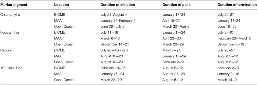
Table 4. Phenology of certain PFT markers in the study region for 2006 as defined by the dates of the initiation, peak and termination of the seasonal maximum/bloom period.
Diatoms were present in highest concentrations along the coasts and dominated the phytoplankton community and were at a minimum during summer in all zones. During spring and summer, values of 19′hexanoyloxyfucoxanthin (prymnesiophytes) peaked, suggesting that they competed better against the diatoms (Figure 8). Diatoms appeared to tolerate deep mixed layers and cool temperatures during their winter maxima in both coastal and open ocean regions (Longhurst, 2010). It appears that their phenology is dependent on both light intensity and photoperiod (Edwards and Richardson, 2004). Diatom spring blooms occur once warming temperatures and weakening winter winds induce upper ocean stratification (Townsend et al., 1994). In late spring (May), diatoms reached their maximal abundance. Edwards and Richardson (2004) reported that this sudden increase is predominantly controlled by light availability in the euphotic zone because the day length and light intensity increase as the degree of mixing gradually declines. The diatoms are the first PFT to be seeded into the phytoplankton community due to their high chlorophyll a per cell with high pigment packaging (Figure 9).
Dinoflagellates showed a similar seasonal trend as the diatoms, but with more variability, especially in the open ocean where their fall bloom was relatively stronger than the higher biomass diatoms. Dinoflagellates were closely linked to temperature with higher concentrations at the coast from December to February, with concentrations decreasing in this region during warm summer months. Dinoflagellate concentrations to ratios peaked in the Gulf of Maine and open ocean around January and decreased in summer. Surprisingly, dinoflagellates appear low in concentration in the Mid Atlantic Bight and showed a dampened seasonality. Dinoflagellates may not only be responding physiologically to temperature, but may also respond to temperature indirectly if stratified conditions appear early in the season (Edwards and Richardson, 2004). The geographic extent of the modeled dinoflagellates in coastal and near coastal cooler waters appeared to contract and expand within a geographic region bounded by sea surface temperatures. A boundary appeared to clearly delineate their distribution between cooler waters that marks the edge of the shelf front to the northwest and the Gulf Stream. This region near the shelf front boundary was the location of the ecotone for the coastal (diatoms) and open ocean phytoplankton populations and also the location for the maximum concentrations of dinoflagellates. It marks the ecotone for the PFTs in the study domain.
Prymnesiophytes (19′hexanoyloxyfucoxanthin), a major feature in the North Atlantic, showed distinct peaks in biomass during the summer (July) with an initiation of their bloom in February at all sites (Holligan et al., 1993). The prymnesiophytes represented in the coastal Mid-Atlantic and open ocean are probably the coccolithophorids, Emiliania huxleyi. Whereas, the Gulf of Maine probably is represented by both coccolithophorids and Phaeocystis. Unfortunately, the marker pigment, 19′hexanoyloxyfucoxanthin, does not differentiate between coccolithophorids and Phaeocystis. However, we hypothesize that Phaeocystis probably blooms in early spring (February) in the Gulf of Maine (Moisan et al., 2013) and reaches its maximal in August. Whereas, coccolithophorids were found in high concentration at the coast and in the open ocean south of the Gulf Stream and peaked in late summer and are dominant feature in remote sensing of Ocean Color (Holligan et al., 1993).
General mechanistic explanations for the phenology of certain PFTs are still controversial, as most phenology has focused on chlorophyll a biomass (Siegel et al., 2002; Ji et al., 2010). Ecological explanations for the presence of individual PFTs include the following: (1) coastal upwelling events, (2) seasonal freshwater fluxes from major estuaries or rivers, (3) variability in the intensity of fall and winter storms which reduce/enhance mixing-induced vertical nutrient fluxes resulting in decreased/increased chlorophyll a levels in fall/winter, and, (4) stronger than usual wind stress curl in the summer, which can shoal the thermocline offshore and deliver nutrients to the upper photic zone, producing local phytoplankton blooms (Foukal and Thomas, 2014). One-dimensional models have proven helpful in revealing the underlying mechanisms driving the phenological shifts in the phytoplankton community when local forcing controls the mixing/stratification dynamics (Olivieri and Chavez, 2000).
Phytoplankton Functional Type Diversity and Climate
A review of the various methods presently in use to estimate PFTs using remote sensing observation (IOCCG, 2014) notes that while it is possible to quantify phytoplankton pigments by differentiation of phytoplankton absorption spectra (Bricaud et al., 2007; Moisan et al., 2011), the requirement for high spectral resolution remote sensing data sets limits its application. A method to estimate various PFTs using hyperspectral observations has been developed (PhytoDOAS, Bracher et al., 2009) that has been able to retrieve global-scale observations of two important PFTs. But, these sophisticated satellite-based applications require hyperspectral data sets. In this study, hyperspectral absorption spectra were modeled as a function of chlorophyll a, using in situ observations of absorption spectra and HPLC pigments. By using an inverse modeling technique to yield pigment estimates from hyperspecral absorption spectra (Moisan et al., 2011, 2013), the method allows us to estimate phytoplankton pigment suites from satellite chlorophyll a measurements. The use of pigment-dependent algorithms to estimate the PFT concentrations (Hirata et al., 2011) demonstrates the potential for developing these types of relationships for various ocean areas. The need to develop such regional relationships was one of the gaps identified by Bracher et al. (2017) in a recent review on obtaining phytoplankton diversity from ocean color data.
The assessment of the PTF diversity patterns in the study domain is the first study that has been done which utilizes a number of techniques to yield PFT estimates from phytoplankton absorption spectra modeled using satellite observations. There are a number of recent studies that have created PFT diversity maps using other techniques, including models. Phytoplankton diversity was compared to primary productivity estimates in the California Current region (Goebel et al., 2013) using an NPZ-type model with 78 phytoplankton types (Goebel et al., 2010). The results from this study calculated the Shannon Diversity Index (H) and species richness and showed that there was very high diversity offshore of the California upwelling regions where production was very high. In addition, north of the west wind drift region H showed very low values in this High Nutrient, Low Chlorophyll region. No clear patterns where observed when comparing H to primary production levels. However the study did note that a number of commonly observed relationships between diversity and productivity did exist, including: monotonic increase; monotonic decrease; a unimodal or hump-backed relationship or a hump-backed envelope that denotes the maximum in the data sets. The results from this study show that non-monotonic diversity versus biomass relationships may exist along the coastal regions of the U.S. east coast, including the Gulf of Maine and extending beyond the shelf front regions where the diversity was estimated to be highest in the areas of the eddy-rich shelf frontal regions. Higher phytoplankton diversity within frontal regions was also calculated in the eddy rich regions of the Gulf Stream Extension (Lévy et al., 2015), which is located due east of this paper's study region. The patterns and locations of the higher H values were similar to those encountered in this study. In this present study highest H values were observed in the frontal regions of the shelf frontal zone and in the central region of the Gulf of Maine, while moderate levels of H offshore can be seen extending eastward with the Gulf Stream extension and contain variability associated with the mesoscale features of the warm core Gulf Stream rings.
Are these satellite-derived estimates of H more informative than the traditional species-resolved H estimates, which the Goebel et al. (2013) and Lévy et al. (2015) studies simulated using a complex species-based model? Does the number of species versus the range of species function determine the functioning capability of the ocean ecosystem? Do we need to know the complexity of species numbers or can we just resolve the functionality of the ecosystem in order to understand it? Some ecologists will argue that both the diversity of the species and the functional types are equally important (Tilman et al., 2001). But a study by Diaz and Cabido (2001) argues that because of the functional nature of the processes that each functional type contributes to ecosystem the functional diversity of the ecosystem is more important to its overall function. Therefore, generating satellite maps of phytoplankton functional diversity even at the course 5-component functional type scale developed in this effort can be useful for monitoring marine ecosystem function over time.
In addition to assessments of the ecosystem function for various ocean regions, maps of PFT diversity can be used to monitor any changes to the ocean's ecosystem over longer time. An analysis of satellite chlorophyll a observations demonstrated that while there is no significant trend in the global scale chlorophyll a levels, there are regions in the ocean where chlorophyll levels have increased and decreased over the SeaWiFS satellite lifetime, 1998-2012 (Gregg et al., 2005; Vantrepotte and Melin, 2009; Henson et al., 2010; Siegel et al., 2013; Gregg and Rousseaux, 2014). Additionally, Boyce et al. (2010) have argued that the ocean's chlorophyll a levels observed have been in decline over the past century. Although this observed decline has been thought to possibly arise from data bias from blending data sets or other errors in the analysis (Mackas, 2011; McQuatters-Gollop et al., 2011; Rykaczewski and Dunne, 2011), any systematic long-term changes in ocean phytoplankton biomass should be reflected in changes to the PFTs and the resulting PFT diversity. An analysis of the local linear trends in the MODIS-Aqua chlorophyll a product from 2002-2016 showed that for the majority of the region used in this study significant trends were observed in about 25% of the domain, with increasing trends in areas along the coast and decreasing chlorophyll levels in the open ocean (Figure 12A). A similar linear trend analysis of the PFT H time series showed that for both those regions the H values had a negative trend (Figure 12B), meaning that diversity decreased in both areas regardless of the fact that the chlorophyll trends were opposite signs in two areas. The reason for this is that the PFT diversity function (Figure 11) shows hump-backed relationship, so that at low chlorophyll values, as observed in the open ocean regions, any decrease in chlorophyll levels leads to a decrease in H, and in the coastal region, where chlorophyll levels are highest an increase in chlorophyll levels also leads to a decrease in H. Such non-linear relationships in the biomass to H relationships can have an interesting impact in the predicted climate scale changes in H.
Conclusion
In summary, the process of inverting modeled phytoplankton absorption spectra generated using satellite chlorophyll observations into biomarker pigments and then utilizing the Hirata et al. (2011) PFT algorithms to estimate PFT diversity demonstrates unique patterns of individual PFTs in the Northwest Atlantic region in addition to large scale and dynamic patterns in PFT diversity. The distribution of the phytoplankton community can be divided into a number of groupings that are all related cross-shelf variability, ranging from coastal ocean to shelf-front/mesoscale-feature dominated, to oligatrophic open ocean regions. The temporal distribution of these PFTs shows phenological variability in these ocean regions, which vary with timing of their seasonal maxima and minima. These regional analyses demonstrate the importance of developing methods to remotely observe PFTs and their H in order to improve knowledge on the temporal and spatial distribution of the major phytoplankton groups and perhaps ecosystem stability at the regional scale, and to potentially quantify the impacts of climate variability on ecosystems. In the future, once greater numbers of global in situ measurements are available, such methods may be expanded to encompass larger areas to serve as a model for analyzing PFTs and diversity trends across the world's oceans. The algorithm's versatility in utilizing available satellite data enables potential applications for providing larger scale estimates to support ecosystem models that attempt to model PFTs explicitly.
Author Contributions
TM was the senior author of the manuscript and contributed to understanding the relationship between absorption and pigmentation in order to understand diversity in the phytoplankton community. TM was an ecologist who sought to understand the linkages between phytoplankton diversity and Carbon Cycle science. She utilized inherent optical properties to link to satellite oceanography to understand biogeochemical cycles in the ocean. KR is a programmer who participated in all of the mathematical calculations that linked phytoplankton optics to community dynamics in the ocean. She is responsible for all of the graphics and calculations for the paper. She is an early oceanographer budding into satellite oceanography. JM is a physical oceanographer and is responsible for formulating the calculations for the biodiversity of phytoplankton. He is responsible for overseeing mathematical calculations and putting them into an ecological framework to understand carbon Cycle Science. His interest is in understanding climate change and how it relates to phytoplankton diversity. ML participated in the collection and processing of samples from ocean cruises. He also worked with JM and TM in developing the matrix inversion algorithms.
Funding
Funding for this research was provided for by the NASA Ocean Biology and Biogeochemistry Research Program, NASA Goddard Space Flight Center, and The Gordon and Betty Moore Foundation. Grant Number 3292 for Gordon and Betty Moore Foundation and 600-14-4316 for Ocean Biology and Biogeochemistry Research Program.
Conflict of Interest Statement
The authors declare that the research was conducted in the absence of any commercial or financial relationships that could be construed as a potential conflict of interest.
Acknowledgments
We thank Ms. Kristin Golmon for earlier testing and development of our inversion algorithm through the NASA USRP Student Program. We thank Carla Makinen and Kristen Blattner participation in filtration and cruise logistics. John Morrow helped to deploy the PRR-800 on several of the BIOME cruises. Our HPLC samples (BIOME, COBY, and MAA cruises) were processed through Laurie van Heukelum (HPEL). The authors wish to thank the Ocean Color Processing Group (OBPG) at the NASA Goddard Space Flight Center (Code 616.0), Greenbelt, Maryland for the production and distribution of the MODIS-Aqua data. We thank our reviewers including Astrid Bracher for their excellent and generous comments that improved our work. Our work was partially funded by the NASA Biodiversity Program 05-TEB/05-0016 and NOAA. The paper was prepared under award #NA03NOS4730220 from NOAA, U.S. Department of Commerce and NASA Climate Adaptation Science Initiative (CASI). The statements, findings, and conclusions are those of the authors and do not necessarily reflect the views of NOAA or the U.S. Department of Commerce.
References
Alvain, S., Moulin, C., and Dandonneau, Y. (2005). Remote sensing of phytoplankton groups in case 1 waters from global SeaWiFS imagery. Deep Sea Res. 52, 1989–2004. doi: 10.1016/j.dsr.2005.06.015
Alvain, S., Moulin, C., Dandonneau, Y., and Loisel, H. (2008). Seasonal distribution and succession of dominant phytoplankton groups in the global ocean: A satellite view. Glob. Biogeochem. Cycles 22, GB3001–GB3015. doi: 10.1029/2007GB003154
Bailey, S. W., and Werdell, P. J. (2006). A multi-sensor approach for the on-orbit validation of ocean color satellite data products. Rem. Sens. Environ. 102, 12–23. doi: 10.1016/j.rse.2006.01.015
Balch, W., Holligan, P. M., Ackleson, S. G., and Voss, K. J. (1991). Biological and optical properties of mesoscale coccolithophore blooms. Limnol. Oceanogr. 36, 629–643. doi: 10.4319/lo.1991.36.4.0629
Balch, W., Kilpatrick, K. A., Holligan, P. M., and Trees, C. (1996). The 1991 coccolithophore bloom in the central north Atlantic I—Optical properties and factors affecting their distribution. Limnol. Oceanogr. 41, 1669–1683. doi: 10.4319/lo.1996.41.8.1669
Barlow, R. G., Mantoura, R. F. C., and Cummings, D. G. (1999). Monsoonal influence on the distribution of phytoplankton pigments in the Arabian Sea. Deep Sea Res. II Top. Stud. Oceanogr. 46, 677–699. doi: 10.1016/S0967-0645(98)00123-4
Barlow, R., Stuart, V., Lutz, V., Sessions, H., Sathyendranath, S., Platt, T., et al. (2007). Seasonal pigment patterns of surface phytoplankton in the subtropical southern hemisphere. Deep Sea Res. I Oceanogr. Res. Pap. 54, 1687–1703. doi: 10.1016/j.dsr.2007.06.010
Bidigare, R. R., Ondrusek, M. E., Morrow, J. H., and Kiefer, D. H. (1990). In vivo absorption properties of algal pigments. Proc. SPIE 1302, 290–302. doi: 10.1117/12.21451
Boyce, D. G., Lewis, M. R., and Worm, B. (2010). Global phytoplankton decline over the past century. Nature 466, 591–596. doi: 10.1038/nature09268
Bracher, A., Bouman, H. A., Brewin, R. J. W., Bricaud, A., Brotas, V., Ciotti, A. M., et al. (2017). Obtaining phytoplankton diversity from ocean color: a scientific roadmap for future development. Front. Mar. Sci. 4:55. doi: 10.3389/fmars.2017.00055
Bracher, A., Taylor, M., Taylor, B., Dinter, T., Roettgers, R., and Steinmetz, F. (2015). Using empirical orthogonal functions derived from remote sensing reflectance for the prediction of phytoplankton pigments concentrations. Ocean Sci. 11, 139–158. doi: 10.5194/os-11-139-2015
Bracher, A., Vountas, M., Dinter, T., Burrows, J. P., Röttgers, R., and Peeken, I. (2009). Quantitative observation of cyanobacteria and diatoms from space using PhytoDOAS on SCIAMACHY data. Biogeosciences 6, 751–764. doi: 10.5194/bg-6-751-2009
Brewin, R., Sathyendranath, S., Hirata, T., Lavender, S., Barciela, R., and Hardman-Mountford, N. (2010). A three-component model of phytoplankton size class for the Atlantic Ocean. Ecol. Modell. 221, 1472–1483. doi: 10.1016/j.ecolmodel.2010.02.014
Bricaud, A., Babin, M., Morel, A., and Claustre, H. (1995). Variability in the chlorophyll-specific absorption coefficients of natural phytoplankton: analysis and parameterization. J. Geophys. Res. 100, 13321–13332. doi: 10.1029/95JC00463
Bricaud, A., Claustre, H., Ras, J., and Oubelkheir, K. (2004). Natural variability of phytoplanktonic absorption in oceanic waters: Influence of the size structure of algal populations. J. Geophys. Res. 109:C11010–1. doi: 10.1029/2004JC002419
Bricaud, A., Mejia, C., Blondeau-Patissier, D., Claustre, H., Crepon, M., and Thiria, S. (2007). Retrieval of pigment concentrations and size structure of algal populations from their absorption spectra using multilayered perceptrons. Appl. Opt. 46, 1251–1260. doi: 10.1364/AO.46.001251
Bruggeman, J., and Kooijman, S. A. L. M. (2007). A biodiversity-inspired approach to aquatic ecosystem modeling. Limnol. Oceanogr. 52:1533. doi: 10.4319/lo.2007.52.4.1533
Campbell, L., Henrichs, D. W., Olson, R. J., and Sosik, H. M. (2013). Continuous automated imaging-in-flow cytometry for detection and early warning of Karenia brevis blooms in the Gulf of Mexico. Environ. Sci. Pollut. Res. 20, 6896–6902. doi: 10.1007/s11356-012-1437-4
Cermeño, P., Dutkiewicz, S., Harris, R. P., Follows, M., Schofield, O., and Falkowski, P. G. (2008). The role of nutricline depth in regulating the ocean carbon cycle. Proc. Natl. Acad. Sci. U.S.A. 105, 20344–20349. doi: 10.1073/pnas.0811302106
Chase, A., Boss, E., Zaneveld, R., Bricaud, A., Claustre, H., Ras, J., et al. (2013). Decomposition of in situ particulate absorption spectra. Methods Oceanogr. 7, 110–124. doi: 10.1016/j.mio.2014.02.002
Ciotti, A. M., Lewis, M. R., and Cullen, J. J. (2002). Assessment of the relationships between dominant cell size in natural phytoplankton communities and the spectral shape of the absorption coefficient. Limnol. Oceanogr. 47, 404–417. doi: 10.4319/lo.2002.47.2.0404
Devred, E., Sathyendranath, S., Stuart, V., and Platt, T. (2011). A three component classification of phytoplankton absorption spectra: Application to ocean-color data. Rem. Sens. Environ. 115, 2255–2266. doi: 10.1016/j.rse.2011.04.025
Diaz, S., and Cabido, M. (2001). Vive le difference: Plant functional diversity matters to ecosystem processes. Trends Evol. 16, 646–655, doi: 10.1016/S0169-5347(01)02283-2
D'Ortenzio, F., and Ribera d'Alcalà, M. (2009). On the trophic regimes of the Mediterranean Sea: a satellite analysis. Biogeosciences 6, 139–148. doi: 10.5194/bg-6-139-2009
Edwards, M., Johns, D. G., Leterme, S. C., Svendsen, E., and Richardson, A. J. (2006). Regional climate change and harmful algal blooms in the northeast Atlantic. Limnol. Oceanogr. 51, 820–829. doi: 10.4319/lo.2006.51.2.0820
Edwards, M., and Richardson, A. J. (2004). Impact of climate change on marine pelagic phenology and trophic mismatch. Nature 430, 881–884. doi: 10.1038/nature02808
Falkowski, P. G., and Raven, J. A. (1997). Aquatic Photosynthesis. Malden, MA: Blackwell Science, 375.
Filippino, K. C., Mulholland, M. R., and Bernhardt, P. W. (2011). Nitrogen uptake and primary productivity rates in the Mid-Atlantic Bight (MAB). Estuar. Coast. Shelf Sci. 91, 13–23. doi: 10.1016/j.ecss.2010.10.001
Foukal, N. P., and Thomas, A. C. (2014). Biogeography and phenology of satellite-measured phytoplankton seasonality in the California current. Deep Sea Res. I Oceanogr. Res. Pap. 92, 11–25. doi: 10.1016/j.dsr.2014.06.008
Garver, S. A., and Siegel, D. A. (1997). Inherent optical property inversion of ocean color spectra and its biogeochemical interpretation: 1. Time series from the Sargasso Sea. J. Geophys. Res. 102, 18607–18625. doi: 10.1029/96JC03243
Geider, R. J., Moore, C. M., and Suggett, D. J. (2014). “Ecology of Marine Phytoplankton,” in Ecology and the Environment, ed R. K. Monson (New York, NY: Springer Science+Business Media), 483–531.
Goebel, N. L., Edwards, C. A., Zehr, J. P., Follow, M. J., and Morgan, S. G. (2013). Modeled phytoplankton diversity and productivity in the California current system. Ecol. Modell. 264, 37–47. doi: 10.1016/j.ecolmodel.2012.11.008
Goebel, N. L., Edwards, C. A., Zehr, J. P., and Follows, M. J. (2010). An emergent community ecosystem model applied to the California current system. J. Mar. Syst. 83, 221–241. doi: 10.1016/j.jmarsys.2010.05.002
Gregg, W. W., Casey, N. W., and McClain, C. R. (2005). Recent trends in global ocean chlorophyll. Geophys. Res. Lett. 32:L03606, doi: 10.1029/2004GL021808
Gregg, W. W., Ginoux, P., Schopf, P. S., and Casey, N. W. (2003). Phytoplankton and iron: validation of a global three-dimensional ocean biogeochemical model. Deep Sea Res. II Top. Stud. Oceanogr. 50, 3143–3169. doi: 10.1016/j.dsr2.2003.07.013
Gregg, W. W., and Rousseaux, C. S. (2014). Decadal trends in global pelagic ocean chlorophyll: a new assessment integrating multiple satellites, in situ data, and models. J. Geophys. Res. 119, 5921–5933. doi: 10.1002/2014jc010158
Hardman-Mountford, N. J., Hirata, T., Richardson, K. A., and Aiken, J. (2008). An objective methodology for the classification of ecological pattern into biomes and provinces for the pelagic ocean. Remote Sens. Environ. 112, 3341–3352. doi: 10.1016/j.rse.2008.02.016
Henson, S. A., Robinson, I., Allen, J. T., and Waniek, J. J. (2006). Effect of meteorological conditions on interannual variability in timing and magnitude of the spring bloom in the Irminger Basin, North Atlantic. Deep Sea Res. I Oceanogr. Res. Pap. 53, 1601–1615. doi: 10.1016/j.dsr.2006.07.009
Henson, S. A., Sarmiento, J. L., Dunne, J. P., Bopp, L., Lima, I., Doney, S. C., et al. (2010), Detection of anthropogenic climate change in satellite records of ocean chlorophyll and productivity, Biogeosciences 7, 621–640. doi: 10.5194/bg-7-621-2010
Hirata, T., Aiken, J., Hardman-Mountford, N., Smyth, T. J., and Barlow, R. G. (2008). An absorption model to determine phytoplankton size classes from satellite ocean colour. Remote Sens. Environ. 112, 3153–3159. doi: 10.1016/j.rse.2008.03.011
Hirata, T., Hardman-Mountford, N., Brewin, R., Aiken, J., Barlow, R., Suzuki, K., et al. (2011). Synoptic relationships between surface Chlorophyll-a and diagnostic pigments specific to phytoplankton functional types. Biogeosciences 8, 311–327. doi: 10.5194/bg-8-311-2011
Hoge, F. E., and Lyon, P. E. (1996). Satellite retrieval of inherent optical properties by linear matrix inversion of oceanic radiance models: an analysis of model and radiance measurement errors. J. Geophys. Res. 101, 16631–16648. doi: 10.1029/96JC01414
Holligan, P. M., Fernández, E., Aiken, J., Balch, W. M., Boyd, P., Burkill, P. H., et al. (1993). A biogeochemical study of the coccolithophore, Emiliania huxleyi, in the North Atlantic. Glob. Biogeochem. Cycles 7, 879–900. doi: 10.1029/93GB01731
Hoogenboom, H. J., Dekker, A. G., and De Haan, J. F. (1998). Retrieval of chlorophyll and suspended matter from imaging spectrometry data by matrix inversion. Can. J. Remote Sens. 24, 144–152. doi: 10.1080/07038992.1998.10855234
Hu, C., Cannizzaro, J., Carder, K. L., Muller-Karger, F. E., and Hardy, R. (2010). Remote detection of Trichodesmium blooms in optically complex coastal waters: Examples with MODIS full-spectra data. Remote Sens. Environ. 114, 2048–2058. doi: 10.1016/j.rse.2010.04.011
Iglesias-Rodriguez, M. D., Halloran, P. R., Rickaby, R. E., Hall, I. R., Colmenero-Hidalgo, E., Gittins, J. R., et al. (2008). Phytoplankton calcification in a high-CO2 world. Science 320, 336–340. doi: 10.1126/science.1154122
IOCCG (2014). Phytoplankton Functional Types from Space. ed S. Sathyendranath, Reports of the International Ocean Colour Coordinating Group, No. 15, IOCCG, (Dartmouth, NS).
Jeffrey, S. W., and Vest, M. (1997). “Introduction to marine phytoplankton and their pigment signatures,” in Phytoplankton Pigments in Oceanography, eds F. S. Jeffrey, F. C. Mantoura, S. W. Wright (Paris: UNESCO), 37–84.
Ji, R., Edwards, M., Mackas, D. L., Runge, J. A., and Thomas, A. C. (2010). Marine plankton phenology and life history in a changing climate: current research and future directions. J. Plankton Res. 32, 1355–1368. doi: 10.1093/plankt/fbq062
Johnsen, G., Samset, O., Granskog, L., and Sakshaug, E. (1994). In-vivo absorption characteristics in 10 classes of bloom-forming phytoplankton-taxonomic characteristics and responses to photoadaptation by means of discriminant and HPLC analysis. Mar. Ecol. Prog. Ser. 105, 149–157. doi: 10.3354/meps105149
Kahru, M., Kudela, R. M., Anderson, C. R., Manzano-Sarabia, M., and Mitchell, B. G. (2014). Evaluation of satellite retrievals of ocean chlorophyll-a in the California Current, Remote Sens., 6, 8524–8540. doi: 10.3390/rs6098524
Kishino, M., Takahashi, M., Okami, N., and Ichimura, S. (1985). Estimation of the spectral absorption coefficients of phytoplankton in the sea. Bull. Mar. Sci. 37, 634–642.
Kostadinov, T. S., Siegel, D. A., and Maritorena, S. (2009). Retrieval of the particle size distribution from satellite ocean color observations. J. Geophys. Res. 114:C09015. doi: 10.1029/2009jc005303
Lawson, C. L., and Hanson, R. J. (1974). Solving Least Squares Problems, Vol. 161, Englewood Cliffs, NJ: Prentice-hall.
Lee, Z., and Carder, K. L. (2004). Absorption spectrum of phytoplankton pigments derived from hyperspectral remote-sensing reflectance. Remote Sens. Environ. 89, 361–368. doi: 10.1016/j.rse.2003.10.013
Levitus, S., Antonov, J. I., Boyer, T. P., and Stephens, C. (2000). Warming of the world ocean. Science 287, 2225–2229. doi: 10.1126/science.287.5461.2225
Lévy, M., Jahn, O., Dutkiewicz, S., Follows, M. J., and d'Ovidio, F. (2015). The dynamical landscape of marine phytoplankton diversity. J. R. Soc. Interface 12:20150481. doi: 10.1098/rsif.2015.0481
Litchman, E., Klausmeier, C. A., Schofield, O. M., and Falkowski, P. G. (2007). The role of functional traits and trade-offs in structuring phytoplankton communities: scaling from cellular to ecosystem level. Ecol. Lett. 10, 1170–1181. doi: 10.1111/j.1461-0248.2007.01117.x
Louanchi, F., and Najjar, R. G. (2001). Annual cycles of nutrients and oxygen in the upper layers of the North Atlantic Ocean. Deep Sea Res. II Top. Stud. Oceanogr. 48, 2155–2171. doi: 10.1016/S0967-0645(00)00185-5
Mackas, D. L. (2011). Does blending of chlorophyll data bias temporal trend? Nature 472, E4–E5, doi: 10.1038/nature09951
Mackey, M. D., Mackey, D. J., Higgins, H. W., and Wright, S. W. (1996). CHEMTAX—a program for estimating class abundances from chemical markers: application to HPLC measurements of phytoplankton. Mar. Ecol. Prog. Ser. 144, 265–283. doi: 10.3354/meps144265
Makinen, C. P., and Moisan, T. A. (2012). Phytoplankton assemblage patterns in the southern Mid-Atlantic Bight. Bot. Mar. 55, 445–457. doi: 10.1515/bot-2012-0110
Marañón, E., Holligan, P. M., Barciela, R., González, N., Mouri-o, B., Paz,ó, M. J., et al. (2001). Patterns of phytoplankton size structure and productivity in contrasting open-ocean environments. Mar. Ecol. Prog. Ser. 216, 43–56. doi: 10.3354/meps216043
Margalef, R. (1978). Life-forms of phytoplankton as survival alternatives in an unstable environment. Oceanologica Acta 1, 493–509.
Marquardt, D. W. (1963). An algorithm for least-squares estimation of nonlinear parameters. J. Soc. Indust. Appl. Math. 11, 431–441. doi: 10.1137/0111030
Marshall, H. G., and Cohn, M. S. (1983). Distribution and composition of phytoplankton in northeastern coastal waters of the United States. Estuar. Coast. Shelf Sci. 17, 119–131. doi: 10.1016/0272-7714(83)90057-4
McGillicuddy, D. J. Jr., Anderson, L. A., Doney, S. C., and Maltrud, M. E. (2003). Eddy-driven sources and sinks of nutrients in the upper ocean: Results from a 0.1° resolution model of the North Atlantic, Global Biogeochem. Cycles 17, 1035. doi: 10.1029/2002GB001987
McQuatters-Gollop, A., Reid, P. C., Edwards, M., Burkill, P. H., Castellani, C., Batten, S., et al. (2011). Is there a decline in marine phytoplankton. Nature 472, E6–E7. doi: 10.1038/nature09950
Mitchell, B. G. (1990). Algorithms for determining the absorption coefficient of aquatic particulates using the quantitative filter technique (QFT). SPIE, Ocean Optics X 1302, 137–148. doi: 10.1117/12.21440
Moisan, J. R., Moisan, T. A., and Linkswiler, M. A. (2011). An inverse modeling approach to estimating phytoplankton pigment concentrations from phytoplankton absorption spectra. J. Geophys. Res. 116:C09018. doi: 10.1029/2010jc006786
Moisan, J. R., Moisan, T. A., Linkswiler, M. A., and Steinhardt, R. A. (2013). Algorithm development for predicting biodiversity based on phytoplankton absorption. Cont. Shelf Res. 55, 17–28. doi: 10.1016/j.csr.2012.12.011
Moisan, T. A., Blattner, K. L., and Makinen, C. P. (2010). Influences of temperature and nutrients on Synechococcus abundance and biomass in the southern Mid-Atlantic Bight. Cont. Shelf Res. 30, 1275–1282. doi: 10.1016/j.csr.2010.04.005
Moisan, T. A., and Mitchell, B. G. (1999). Photophysiological acclimation of Phaeocystis antarctica Karsten under light limitation. Limnol. Oceanogr. 44, 247–258. doi: 10.4319/lo.1999.44.2.0247
Moisan, T. A., and Mitchell, B. G. (2001). UV absorption by mycosporine-like amino acids in Phaeocystis antarctica Karsten induced by photosynthetically available radiation. Mar. Biol. 138, 217–227. doi: 10.1007/s002270000424
Morel, A., and Bricaud, A. (1981). Theoretical results concerning light absorption in a discrete medium, and application to specific absorption of phytoplankton. Deep Sea Res. A Oceanogr. Res. Pap. 28, 1375–1393. doi: 10.1016/0198-0149(81)90039-X
Mouw, C. B., and Yoder, J. A. (2005). Primary production calculations in the Mid-Atlantic Bight, including effects of phytoplankton community size structure. Limnol. Oceanogr. 50, 1232–1243. doi: 10.4319/lo.2005.50.4.1232
Mouw, C. B., and Yoder, J. A. (2010). Optical determination of phytoplankton size composition from global SeaWiFS imagery. J. Geophys. Res. 115:C12018. doi: 10.1029/2010jc006337
Mouw, C. B., Yoder, J. A., and Doney, S. C. (2012). Impact of phytoplankton community size on a linked global ocean optical and ecosystem model. J. Mar. Syst. 89, 61–75. doi: 10.1016/j.jmarsys.2011.08.002
Nair, A., Sathyendranath, S., Platt, T., Morales, J., Stuart, V., Forget, M. H., et al. (2008). Remote sensing of phytoplankton functional types. Remote Sens. Environ. 112, 3366–3375. doi: 10.1016/j.rse.2008.01.021
Navarro, G., Alvain, S., Vantrepotte, V., and Huertas, I. E. (2014). Identification of dominant phytoplankton functional types in the Mediterranean Sea based on a regionalized remote sensing approach. Remote Sens. Environ. 152, 557–575. doi: 10.1016/j.rse.2014.06.029
Oliver, M. J., and Irwin, A. J. (2008). Objective global ocean biogeographic provinces. Geophys. Res. Lett. 35:L15601. doi: 10.1029/2008GL034238
Olivieri, R. A., and Chavez, F. P. (2000). A model of plankton dynamics for the coastal upwelling system of Monterey Bay, California. Deep-Sea Res. II 47, 1077–1106. doi: 10.1016/S0967-0645(99)00137-X
O'Reilly, J. E., and Zetlin, C. (1998). Seasonal, Horizontal, and Vertical Distribution of Phytoplankton Chlorophyll a in the Northeast US Continental Shelf Ecosystem. NOAA Technical Report NMFS, 139.
Organelli, E., Bricaud, A., Antoine, D., and Uitz, J. (2013). Multivariate approach for the retrieval of phytoplankton size structure from measured light absorption spectra in the Mediterranean Sea (BOUSSOLE site). Appl. Opt. 52, 2257–2273. doi: 10.1364/AO.52.002257
Ornótfsdóttir, E. B., Pinckney, J. L., and Tester, P. A. (2003). Quantification of the relative abundance of the toxic dinoflagellate, Karenia brevis (Dinophyta), using unique photopigments. J. Phycol. 39, 449–457. doi: 10.1046/j.1529-8817.2003.01219.x
Pan, X., Mannino, A., Marshall, H., Filippino, K., and Mulholland, M. (2011). Remote sensing of phytoplankton community composition along the northeast coast of the United States. Remote Sens. Environ. 115, 3731–3747. doi: 10.1016/j.rse.2011.09.011
Pan, X., Mannino, A., Russ, M., Hooker, S., and Harding, L. (2010). Remote sensing of phytoplankton pigment distribution in the United States northeast coast. Remote Sens. Environ. 114, 2403–2416. doi: 10.1016/j.rse.2010.05.015
Platt, T., and Sathyendranath, S. (2008). Ecological indicators for the pelagic zone of the ocean from remote sensing. Remote Sens. Environ. 112, 3426–3436. doi: 10.1016/j.rse.2007.10.016
Platt, T., White, G. N., Zhai, L., Sathyendranath, S., and Roy, S. (2009). The phenology of phytoplankton blooms: ecosystem indicators from remote sensing. Ecol. Model. 220, 3057–3069. doi: 10.1016/j.ecolmodel.2008.11.022
Press, W. H., Flannery, B. P., Teukolsky, S. A., Vetterling, W. T., and Gould, H. (1987). Numerical recipes, the art of scientific computing. Am. J. Phys. 55, 90–91. doi: 10.1119/1.14981
Raitsos, D. E., Lavender, S. J., Maravelias, C. D., Haralabous, J., Richardson, A. J., and Reid, P. C. (2008). Identifying four phytoplankton functional types from space: an ecological approach. Limnol. Oceanogr. 53, 605–613. doi: 10.4319/lo.2008.53.2.0605
Roy, S., Llewellyn, C., Egeland, E., and Johnsen, G. (eds.). (2011). Phytoplankton Pigments: Characterization, Chemotaxonomy and Applications in Oceanography. Cambridge: Cambridge University Press, 845.
Roy, S., Sathyendranath, S., Bouman, H., and Platt, T. (2013). The global distribution of phytoplankton size spectrum and size classes from their light-absorption spectra derived from satellite data. Remote Sens. Environ. 139, 185–197. doi: 10.1016/j.rse.2013.08.004
Rykaczewski, R. R., and Dunne, J. P. (2011). A measured look at ocean chlorophyll trends. Nature 472, E5–E6, doi: 10.1038/nature09952
Sadeghi, A., Dinter, T., Vountas, M., Taylor, B., Altenburg-Soppa, M., and Bracher, A. (2012). Remote sensing of coccolithophore blooms in selected oceanic regions using the PhytoDOAS method applied to hyper-spectral satellite data. Biogeosciences 9, 2127–2143. doi: 10.5194/bg-9-2127-2012
Sarmiento, J. L., Gruber, N., Brzezinski, M. A., and Dunne, J. P. (2004). High-latitude controls of thermocline nutrients and low latitude biological productivity. Nature 427, 56–60. doi: 10.1038/nature02127
Sathyendranath, S., Watts, L., and Devred, E. (2004). Discrimination of diatoms from other phytoplankton using ocean-colour data. Mar. Ecol. Prog. Ser. 272, 59–68. doi: 10.3354/meps272059
Schoemann, V., Becquevort, S., Stefels, J., Rousseau, V., and Lancelot, C. (2005). Phaeocystis blooms in the global ocean and their controlling mechanisms: a review. J. Sea Res. 53, 43–66. doi: 10.1016/j.seares.2004.01.008
Shannon, C. E. (1948). A mathematical theory of communication. Bell Syst. Techn. J. 27, 379–423. doi: 10.1002/j.1538-7305.1948.tb01338.x
Siegel, D. A., Behrenfeld, M. J., Maritorena, S., McClain, C. R., Antoined, D., Bailey, S. W., et al. (2013). Regional to global assessments of phytoplankton dynamics from the SeaWiFS mission. Remote Sens. Environ. 135, 77–91. doi: 10.1016/j.rse.2013.03.025
Siegel, D. A., Doney, S. C., and Yoder, J. A. (2002). The North Atlantic spring phytoplankton bloom and Sverdrup's critical depth hypothesis. Science 296, 730–733. doi: 10.1126/science.1069174
Sommer, U., Padisak, J., Renolds, C. S., and Juhasz-Nagy, P. (1993). Hutchinson's heritage: the diversity-disturbance relationship in phytoplankton. Hydrobiologia 249, 1–7. doi: 10.1007/BF00008837
Soppa, M., Hirata, T., Silva, B., Dinter, T., Peeken, I., Wiegmann, S., et al. (2014). Global retrieval of diatom abundance based on phytoplankton pigments and satellite data. Remote Sens. 6, 10089–10106. doi: 10.3390/rs61010089
Stramma, L., and Siedler, G. (1988). Seasonal changes in the North Atlantic subtropical gyre. J. Geophys. Res. 93, 8111–8118. doi: 10.1029/JC093iC07p08111
Striebel, M., Behl, S., and Stibor, H. (2009). The coupling of biodiversity and productivity in phytoplankton communities: consequences for biomass stoichiometry. Ecology 90, 2025–2031. doi: 10.1890/08-1409.1
Subramaniam, A., Brown, C. W., and Hood, R. R. (2002). Detecting Trichodesmium blooms in SeaWiFS imagery. Deep-Sea Res. II 49, 107–121. doi: 10.1016/S0967-0645(01)00096-0
Subramaniam, A., and Carpenter, E. J. (1994). An empirically derived protocol for the detection of blooms of the marine cyanobacterium Trichodesmium using CZCS imagery. Int. J. Remote Sens. 158, 1559–1569. doi: 10.1080/01431169408954191
Subramaniam, A., Carpenter, E. J., Karentz, P. G., and Falkowski, P. G. (1999a). Optical properties of the marine diazotrophic cyanobacteria Trichodesmium spp. I. Absorption and spectral photosynthetic characteristics. Limnol. Oceanogr. 44, 608–617. doi: 10.4319/lo.1999.44.3.0608
Subramaniam, A., Carpenter, E. J., and Falkowski, P. G. (1999b). Optical properties of the marine diazotrophic cyanobacteria Trichodesmium spp. II. Reflectance model for remote sensing. Limnol. Oceanogr. 44, 618–627. doi: 10.4319/lo.1999.44.3.0618
Terseleer, N., Bruggeman, J., Lancelot, C., and Gypens, N. (2014). Trait-based representation of diatom functional diversity in a plankton functional type model of the eutrophied southern North Sea. Limnol. Oceanogr. 59, 1958–1972. doi: 10.4319/lo.2014.59.6.1958
Thomas, A. C., Townsend, D. W., and Weatherbee, R. (2003). Satellite-measured phytoplankton variability in the Gulf of Maine. Cont. Shelf Res. 23, 971–989. doi: 10.1016/S0278-4343(03)00086-4
Tilman, D., Reich, P. B., Knops, J., Wedin, D., Mielke, T., and Lehman, C. (2001). Diversity and productivity in a long-term grassland experiment. Science 294, 843–845. doi: 10.1126/science.1060391
Townsend, D. W., Cammen, L. M., Holligan, P. M., Campbell, D. E., and Pettigrew, N. R. (1994). Causes and consequences of variability in the timing of spring phytoplankton blooms. Deep Sea Res. I Oceanogr. Res. Pap. 41, 747–765. doi: 10.1016/0967-0637(94)90075-2
Ueyama, R., and Monger, B. C. (2005). Wind-induced modulation of seasonal phytoplankton blooms in the North Atlantic derived from satellite observations. Limnol. Oceanogr. 50, 1820–1829. doi: 10.4319/lo.2005.50.6.1820
Uitz, J., Claustre, H., Morel, A., and Hooker, S. B. (2006). Vertical distribution of phytoplankton commu,ities in open ocean: An assessment based on surface chlorophyll. J. Geophys. Res. 111:C08005. doi: 10.1029/2005JC003207
Van Heukelem, L., Thomas, C. M., and Gilbert, P. M. (2002). “Sources of variability in chlorophyll analysis by fluorometry and high performance liquid chromatography in a SIMBIOS inter-calibration exercise,” in NASA Technical Memorandum 2002-211606. Greenbelt, MD: Goddard Space Flight Center, 50.
Vantrepotte, V., and Melin, F. (2009). Temporal variability of 10-year global SeaWiFS time-series of phytoplankton chlorophyll a concentration. ICES J. Mar. Sci. 66, 1547–1556. doi: 10.1093/icesjms/fsp107
Verity, P. G., Brussaard, C. P., Nejstgaard, J. C., van Leeuwe, M. A., Lancelot, C., and Medlin, L. K. (2007). Current understanding of Phaeocystis ecology and biogeochemistry, and perspectives for future research. Biogeochemistry 83, 311–330. doi: 10.1007/s10533-007-9090-6
Vidussi, F., Claustre, H., Manca, B. B., Luchetta, A., and Marty, J. C. (2001). Phytoplankton pigment distribution in relation to upper thermocline circulation in the eastern Mediterranean Sea during winter. J. Geophys. Res. 106, 19939–19956. doi: 10.1029/1999JC000308
Walther, G. R., Post, E., Convey, P., Menzel, A., Parmesan, C., Beebee, T. J. C., et al. (2002). Ecological responses to recent climate change. Nature 416, 389–395. doi: 10.1038/416389a
Wang, G., Lee, Z., Mishra, D. R., and Ma, R. (2016). Retrieving absorption coefficients of multiple phytoplankton pigments from hyperspectral remote sensing reflectance measured over cyanobacteria bloom waters. Limnol. Oceanogr. 14, 432–447. doi: 10.1002/lom3.10102
Welschmeyer, N. A. (1994). Fluorometric analysis of chlorophyll a in the presence of chlorophyll b and pheopigments. Limnol. Oceanogr. 39, 1985–1992. doi: 10.4319/lo.1994.39.8.1985
Werdell, P. J., and Bailey, S. W. (2005). An improved in-situ bio-optical data set for ocean color algorithm development and satellite data product validation. Remote Sens. Environ. 98, 122–140. doi: 10.1016/j.rse.2005.07.001
Whitehead, K., and Vernet, M. (2000). Influence of mycosporine-like amino acids (MAAs) on UV absorption by particulate and dissolved organic matter in La Jolla Bay. Limnol. Oceanogr. 45, 1788–1796. doi: 10.4319/lo.2000.45.8.1788
Woodward, E. M. S., and Rees, A. P. (2001). Nutrient distributions in an anticyclonic eddy in the northeast Atlantic Ocean, with reference to nanomolar ammonium concentrations. Deep Sea Res. II. 48. 775–793. doi: 10.1016/S0967-0645(00)00097-7
Wright, S. W. (2005). Analysis of Phytoplankton Populations Using Pigment Markers. Workshop of pigment analysis of Antarctic microorganisms, University of Malaya, June 20-July 1.
Keywords: phytoplankton, absorption, diversity, phytoplankton functional type, phytoplankton community, pigments, biodiversity, climate change
Citation: Moisan TA, Rufty KM, Moisan JR and Linkswiler MA (2017) Satellite Observations of Phytoplankton Functional Type Spatial Distributions, Phenology, Diversity, and Ecotones. Front. Mar. Sci. 4:189. doi: 10.3389/fmars.2017.00189
Received: 31 March 2017; Accepted: 31 May 2017;
Published: 19 June 2017.
Edited by:
Astrid Bracher, Alfred-Wegener-Institute Helmholtz Center for Polar and Marine Research, GermanyReviewed by:
Hongyan Xi, Helmholtz-Zentrum Geesthacht Centre for Materials and Coastal Research (HZG), GermanyGuoqing Wang, University of Massachusetts System, United States
Copyright © 2017 Moisan, Rufty, Moisan and Linkswiler. This is an open-access article distributed under the terms of the Creative Commons Attribution License (CC BY). The use, distribution or reproduction in other forums is permitted, provided the original author(s) or licensor are credited and that the original publication in this journal is cited, in accordance with accepted academic practice. No use, distribution or reproduction is permitted which does not comply with these terms.
*Correspondence: John R. Moisan, am9obi5yLm1vaXNhbkBuYXNhLmdvdg==
†Deceased 5 June, 2016.