Limited Spatial and Temporal Variability in Meiofauna and Nematode Communities at Distant but Environmentally Similar Sites in an Area of Interest for Deep-Sea Mining

Pape, Ellen; Bezerra, Tania N.; Hauquier, Freija; Vanreusel, Ann

doi:10.3389/fmars.2017.00205

ORIGINAL RESEARCH article

Front. Mar. Sci., 29 June 2017

Sec. Deep-Sea Environments and Ecology

Volume 4 - 2017 | https://doi.org/10.3389/fmars.2017.00205

This article is part of the Research Topic Anthropogenic Disturbances in the Deep Sea View all 18 articles

Limited Spatial and Temporal Variability in Meiofauna and Nematode Communities at Distant but Environmentally Similar Sites in an Area of Interest for Deep-Sea Mining

$\r\nEllen Pape*$ Ellen Pape^*

Tania N. Bezerra

Freija Hauquier

Ann Vanreusel

Marine Biology Research Group, Ghent University, Ghent, Belgium

To be able to adequately assess potential environmental impacts of deep-sea polymetallic nodule mining, the establishment of a proper environmental baseline, incorporating both spatial and temporal variability, is essential. The aim of the present study was to evaluate both spatial and intra-annual variability in meiofauna (higher taxa) and nematode communities (families and genera, and Halalaimus species) within the license area of Global Sea mineral Resources (GSR) in the northeastern Clarion Clipperton Fracture Zone (CCFZ), and to determine the efficiency of the current sampling of meiofauna and nematode diversity. In October 2015, three polymetallic nodule-bearing sites, about 60–270 km apart, located at similar depths (ca. 4,500 m) were sampled, of which one site was sampled in April in that same year. Despite the relatively large geographical distances and the statistically significant, but small, differences in sedimentary characteristics between sites, meiofauna and nematode communities were largely similar in terms of abundance, composition and diversity. Between-site differences in community composition were mainly driven by a set of rare and less abundant taxa. Moreover, although surface primary productivity in April exceeded that in October, no significant changes were observed in sedimentary characteristics or in meiofauna and nematode communities. At all sites and in both periods, Nematoda were the prevailing meiofaunal phylum, which was in turn dominated by Monhysterid genera and Acantholaimus. Our findings support the earlier purported notion of a low degree of endemism for nematode genera and meiofauna taxa in the deep sea, and hint at the possibility of large distribution ranges for at least some Halalaimus species. Taxon richness estimators revealed that the current sampling design was able to characterize the majority of the meiofauna and nematode taxa present. To conclude, implications of the present findings for environmental management and future research needs are provided.

Introduction

The deep-sea bed (>200 m water depth) constitutes the largest benthic ecosystem on Earth (Tyler et al., 2016). Nevertheless, although deep-sea sampling efforts have surged in recent years (Stuart et al., 2008; McClain and Schlacher, 2015), the deep-sea floor, and especially the abyss (>3,000 m; Stuart et al., 2008), remains largely undersampled (Ramirez-Llodra et al., 2010). Moreover, there are relatively few high-resolution temporal (i.e., intra-annual) biological data collected in the deep sea (Galeron et al., 2001; Veit-Köhler et al., 2011; Guilini et al., 2013; Lins et al., 2014), which is linked to its remoteness and the consequently high financial cost associated with deep-sea sampling. As a consequence, our comprehension of the level of biodiversity, as well as of the degree of spatial and temporal variability in benthic community composition and biodiversity in the deep sea, and the responsible drivers, is still incomplete (Rex and Etter, 2010; McClain and Schlacher, 2015). In the last decades, human exploitation activities, including fisheries, and oil and gas exploration, are expanding progressively to offshore, deeper waters in response to an increasing demand for biological and mineral resources, and to technological innovations (Glover and Smith, 2003; Ramirez-Llodra et al., 2011). Unfortunately, our inadequate knowledge about the structure and dynamics of the deep-sea benthic ecosystem, hinders the accurate prediction (prior to exploitation) or evaluation (following exploitation) of the environmental impacts that may arise from these activities.

One exploitation activity that may potentially take place in the near future is the mining of polymetallic nodules (Clark et al., 2013). Polymetallic nodules, potato-shaped accretions rich in commercially interesting metals, occur at abyssal depths underneath low-productive waters. The Clarion Clipperton Fracture Zone (CCFZ) in the northeast Pacific is considered to harbor one of the largest high-grade nodule reservoirs and has therefore gained the most attention from industries and governments (Lodge et al., 2014). The first contracts for the exploration of polymetallic nodules in the CCFZ were granted by the International Seabed Authority (ISA) in 2001, and currently 15 license areas have been assigned (https://www.isa.org.jm/deep-seabed-minerals-contractors). Contractors are required to collect environmental data to establish an environmental baseline, incorporating both spatial and temporal variability, against which to assess the likely effects of their activities on the marine environment (ISA, 2002, 2013).

Meiofauna (>32 μm) is the most abundant and one of the most diverse components of the metazoan benthos in the deep sea (Sinniger et al., 2016) including the CCFZ (Smith and Demopoulos, 2003). Studies investigating temporal and/or spatial trends in meiofaunal communities in the CCFZ are limited to the 9°N and 5°N “EqPac” stations (Lambshead et al., 2003) and four currently assigned license areas, i.e., IOM¹ (Radziejewska et al., 2001), IFREMER² (Mahatma, 2009; Miljutina et al., 2010; Miljutin et al., 2015), DORD³ (Kaneko et al., 1997; Shirayama and Fukushima, 1997) and CIIC⁴ (Trueblood and Ozturgut, 1997; study conducted by the National Oceanographic and Atmospheric Administration's Ocean Minerals and Energy Division; see also the meta-analytical papers by Vanreusel et al., 2010; Radziejewska, 2014; Singh et al., 2016 and the paper by Jones et al., 2017). Temporal variability in CCFZ meiofauna was so far only assessed by comparing different years (Trueblood and Ozturgut, 1997; Shirayama, 1999; Radziejewska et al., 2001). Also for the mega-, macro-, and micro-fauna intra-annual variability in the CCFZ remains to be evaluated.

In this study, samples were collected in the license area of Global Sea mineral Resources (GSR) in the northeastern CCFZ, to evaluate both spatial and intra-annual variability in meiofauna and nematode communities. To this end, three nodule-bearing sites at similar depths (ca. 4,500 m) were sampled (between roughly 60 and 270 km apart), of which one was sampled during two different cruises in 2015 (April-May: SO239, September-October: GSRNOD15A). As these three sites are of potential interest for deep-sea mining, the results presented here are of direct relevance to environmental (spatial) management which aims, amongst others, at preserving biodiversity. Information on the level of biodiversity, as well as on the distribution ranges and connectivity of taxa, will aid in the delineation of impact reference zones (IRZs, to evaluate impacts of mining) and preservation reference zones (PRZs, to protect certain taxa or to allow for mitigation of mining-induced alterations in biodiversity) within the license area (ISA, 2013). Both types of reference zones need to be similar in faunal abundance, composition and diversity to the targeted mine site, and the PRZs also need to be positioned as such as to allow for recolonization of the targeted mine sites (ISA, 2013). Specifically, the following questions were addressed here:

• Do similarly deep nodule-bearing sediments (i.e., similar macro-habitats) separated by more than 60–270 kms harbor similar meiofauna and nematode communities in terms of abundance, composition and diversity?

• Do meiofauna and nematode communities at 4,500 m water depth display intra-annual variability?

• What portion of meiofauna and nematode diversity is characterized by the current sampling?

Materials and Methods

Study Area

The Clarion Clipperton Zone (CCFZ), that part of the Pacific abyss bounded by the Clarion and Clipperton fracture zones (see Figure 1), is located in the Eastern Tropical Pacific (ETP). Primary productivity in the ETP is moderate but the region displays considerable spatio-temporal variability (Pennington et al., 2006). Both longitudinal and latitudinal gradients in surface water production and the resultant flux of particulate organic carbon (POC) to the seafloor have been observed in the CCFZ (Smith et al., 1997; Wedding et al., 2013). Interannual variability in primary productivity is driven by interannual El Niño-Southern Oscillations (ENSO) and multidecadal Pacific Decadal Oscillations (though the effects are strongest near the equator, in eastern coastal boundary regions, and in the central north Pacific; Fiedler, 2002), but also global warming is thought to affect primary productivity in the ETP (Behrenfeld et al., 2006). In contrast, intra-annual variability is considered to be relatively low (Amos and Roels, 1977; Pennington et al., 2006).

FIGURE 1

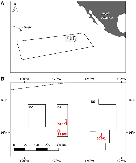
Figure 1. (A) Location of the Clarion Clipperton Fracture Zone (CCFZ); coordinates based on the working definition of Glover et al. (2015) with an indication of the GSR license area. (B) Location of the three sites sampled within the GSR license area during GSRNOD15A (in red). Site B6S02 was also sampled for meiofauna and environmental variables during cruise SO239.

In 2013, the Belgian company GSR was granted a license for the exploration for polymetallic nodules in the CCFZ by the International Seabed Authority for an area of 76,728 km². The GSR license area, located in the northeast of the CCFZ, is divided in three non-adjacent zones, called B2, B4, and B6. During the exploration cruise in 2015 (termed GRSNOD15A), three sites (each ca. 10 × 20 km) were targeted, of which two are located in B4 (B4S03 and B4N01) and one in B6 (B6S02). Samples for meiofauna (including nematodes) and sediment environmental variables (i.e., bacterial biomass and sediment characteristics) were collected in the frame of a biological baseline study to characterize spatial and intra-annual variability.

Sampling Strategy and Onboard Sample Processing

At each site, sediments were sampled in triplicate with a multicorer (MUC) aboard the RV Mt. Mitchell during the GSRNOD15A cruise (September-October 2015) to the GSR license area (see Table 1). At site B6S02, MUC001–MUC003 were deployed at approximately the same locations as those of MUC deployments 121, 124, and 146, respectively, done during the JPI Oceans aboard the RV Sonne which took place in April–May 2015 (i.e., cruise SO239; Haeckel and Arbizu, 2015). This sampling strategy allowed for the evaluation of intra-annual or seasonal variability in sediment characteristics and in meiofauna and nematode communities at this site (SO239 samples were not analyzed for bacterial biomass). Given the sampling dates (see Table 1), the SO239 MUC samples collected at site B6S02 will be referred to as the “April 2015” samples, whilst the GSRNOD15A MUC samples from B6S02 will be designated as the “October 2015” samples. Per MUC deployment, 1 core was analyzed for meiofauna and nematode community attributes, whilst another core was studied for sediment characteristics. During GSRNOD15A, two additional cores from each MUC deployment were sampled for the quantification of sediment bacterial biomass and phytopigments. Unfortunately, the high-performance liquid chromatography (HPLC) analysis (following Wright and Jeffrey, 1997; Van Heukelem and Thomas, 2001) of the sediment samples yielded concentrations below the detection limit (< 20 ng g⁻¹). The MUC aboard the RV Sonne and the RV Mt. Mitchell had an internal diameter of 94 and 100 mm, respectively. From MUC124 (obtained during the SO239 cruise), no core was available for the study of sediment characteristics. Hence, to evaluate intra-annual variability in sediment characteristics at site B6S02, we analyzed data from one of the cores from MUC125 (Table 1). Sediment cores were processed in a cold lab container which was set at 4°C, close to the in situ bottom water temperature. From the cores intended for meiofauna analysis, the 5 cm of water standing on top of the sediment as well as the top 0–5 cm of the sediment were added to one sample container. To each sediment sample a roughly equal amount of 10% seawater-buffered formaldehyde was added. Sediment cores intended for the analysis of bacterial biomass (GSRNOD15A) and sediment characteristics (SO239 and GSRNOD15A) were sliced vertically (GSRNOD15A: per cm to 5 cm depth, SO239: 0–1 cm, 1–5 cm) and stored at −20°C till further analysis.

TABLE 1

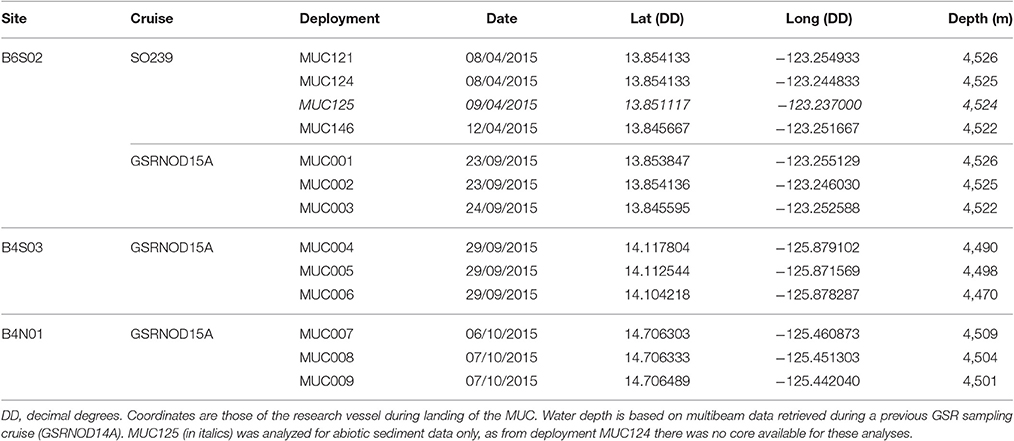
Table 1. Details of the multicorer (MUC) deployments during sampling cruises GSRNOD15A (October 2015) and SO239 (April 2015).

Sample Analysis

Analysis of Environmental Variables

To determine whether the difference in the timing of sampling (April vs. October 2015) was associated with a difference in surface net primary productivity (NPP), we extracted Vertically Generalized Production Model (VGPM) estimated NPP (Behrenfeld and Falkowski, 1997) based on MODIS data for site B6S02 for January 2015–October 2015. Monthly-averaged NPP values were downloaded in HDF format from the Ocean Productivity website (http://www.science.oregonstate.edu/ocean.productivity/index.php) and converted to geotiff using the SeaDAS software. In QGIS, the point sampling tool was used to extract NPP values for all MUC deployment locations. Monthly NPP values for B6S02 were calculated as the average NPP over all deployments.

Sediments were weighed before and after drying (60°C) to determine water content, which was in turn used to estimate porosity, assuming a dry sediment density of 2.55 g cm⁻³. Grain size analysis of ca. 1 g of sediment was performed with a Malvern Mastersizer hydro 2000 G. The granulometric variables used in this study to describe the physical environment of the meiobenthos were: median grain size (MGS), the percentage of sand (grain size > 63 μm), clay (grain size < 4 μm), and silt (4 μm < grain size < 63 μm; Wentworth, 1922), and the sediment sorting coefficient (SC). SC, which is a measure for the spread distance of the various grain sizes, was calculated following Giere (2009). Total organic carbon (TOC) and total nitrogen (TN) content were measured on 200 mg samples using a Flash 2000 NC Sediment Analyser of Interscience (Thermo scientific) after acidification with 1% HCl to remove inorganic carbon.

Per 1-cm sediment layer (0–5 cm), lipids were extracted from ca. 3 g of freeze-dried sediment using a modified Bligh and Dyer (1959) method (Boschker et al., 1999). The polar lipid fraction was obtained by fractionation on silicic acid, and derivatized using mild alkaline methanolysis to yield fatty acid methyl esters (FAMEs). The concentration of these FAMEs was determined with a gas chromatograph-mass spectrometer (GC-MS) from Agilent (GC-6890N + MS-5973N). Samples were run in splitless mode (1 μl injection per run, injector temperature of 250°C) using a HP-88 column (Agilent J&W, 0.2 mm internal diameter × 60 m) with a He flow rate at constant pressure. The FAME C19:0 (Fluka 74208) was added as an internal standard. Oven temperature was initially set at 50°C for 2 min, followed by a ramp at 25°C min⁻¹ to 75°C, and then a second and final ramp at 2°C min⁻¹ to 230°C with a final 4 min hold. FAMEs were identified by comparing the retention times and mass spectra with those of two external standards, i.e., the Bacterial Acid Methyl Esters Mix (Sigma-Aldrich, catalog #47080-U) and the Supelco 37 component FAME mix (Sigma-Aldrich, Supelco #47885), and available ion spectra in the WILEY and a self-constructed library. These analyses were done using the software MSD ChemStation by Agilent Technologies. Individual FAMEs were quantified by linearly regressing the chromatographic peak areas against known concentrations of the standards in the Supelco 37 component FAME mix. Bacteria-specific phospholipid-derived fatty acids (PLFAs) that were present in all of our samples were i15:0, a15:0, and i16:0. As these PLFAs make up roughly 13% of all bacterial PLFAs (based on literature sources mentioned by Middelburg et al. (2000), and 5.6% of the total carbon content in bacterial cells represents PLFA carbon (Brinch-Iversen and King, 1990), the concentrations of these three PLFAs enabled the estimation of bacterial biomass. PLFA concentrations were measured per unit weight of sediment but were converted to unit surface area taking into account sediment porosity.

Analysis of Meiofauna and Nematodes

Sediments were washed over a 32 μm sieve (no upper sieve was used), and the sieve residue was subjected to three Ludox centrifugation rounds to extract the meiofauna (Burgess, 2001). After the last round, the supernatant was poured over a 32 μm sieve and the sieve residue was stored in borax-buffered 4% formaldehyde. Next, a drop of a 1% Rose Bengal-formaldehyde solution was added to stain the organic material, facilitating recognition of meiofauna. Metazoan meiofauna (hereafter referred to as “meiofauna”) was sorted, enumerated, and identified at higher taxonomic level using a stereomicroscope following Higgins and Thiel (1988). Meiofauna counts were converted to abundances per surface area as ind. 10 cm⁻², which is commonly done in ecological meiofauna studies. To account for differences in sediment volume caused by the presence of nodules, we estimated sediment volume of each MUC sample (0–5 cm) by (1) assessing the volume of meiofauna extraction residues (>32 μm) using a measuring cylinder and, (2) calculating the volumetric fraction of the sediment with a grain size < 32 μm based on granulometric analyses. Per sample about 120 nematodes were hand-picked at random, mounted on slides, and identified to family and genus level (where possible). Additionally, the life stage/gender was noted if possible (female/male/juvenile). Some genera are hard to distinguish based on morphological characteristics, especially when dealing with juveniles (e.g., Thalassomonhystera/Monhystrella, and Microlaimus/Aponema), so these were pooled in so-called genus groups. Halalaimus was further identified down to species level because of (1) the relatively high relative abundance of this genus at each site (2) the pre-existence of molecular data for Halalaimus sampled in the CCFZ, including the GSR license area, which can at a later stage be linked to the morphological data. Specimens that resembled but were not morphologically identical to a certain taxon, were designated as “aff” to assign the morphological affinity with that taxon.

Data Analysis

For each sample, diversity was evaluated for meiofauna higher taxa, nematode families and nematode genera using the following indices: taxon richness (higher meiofauna taxa: T, nematode families: F, nematode genera: G), Pielou's evenness (J'), Shannon–Wiener diversity (H'), expected taxon richness for a sample of 51 individuals [higher taxa: ET(51), nematode families: EF(51), nematode genera: EG(51)]. For Halalaimus species, diversity was only assessed in terms of species richness (S) because of the small sample size. Moreover, taxon-accumulation curves (TACs), plotting the cumulative number of taxa observed (T_obs) as a function of the number of sites/samples or periods studied, were produced for all taxonomical levels by randomly adding sites/samples or periods and repeating this procedure 9999 times. Additionally, the non-parametric Chao1 (determined by the number of taxa that have only one or two individuals in the complete sample set), Jacknife2 (“jack2;” a function of the number of taxa retrieved in one or two samples) and Bootstrap (“boot;” dependent on the set of proportions of samples that contain each taxon) estimators (see also Magurran, 2004; Gotelli and Colwell, 2010) were used to extrapolate the TACs to obtain an estimate of total taxon richness in the GSR license area. The usage of non-parametric estimators to estimate the (minimal) total number of taxa present was recommended by Gotelli and Colwell (2010). The comparison of T_obs and the taxon richness estimators allowed for an estimation of the percentage of total taxon richness characterized by our sampling strategy for all taxonomical levels considering all MUC samples and all sites. In addition, the minimum number of additional samples required to detect 95 and 100% of the estimated asymptotic taxon richness was calculated using the non-parametric method based on taxon counts (Chao1) sensu Chao et al. (2009). The average number of individuals identified per sample was used to estimate the additional number of samples needed.

Differences between sites and periods regarding sedimentary environmental variables, total meiofauna abundance, diversity indices, and meiofauna and nematode community composition were examined using a one-way PERMANOVA analysis with “site” (levels: B6S02, B4S03 and B4N01) or “period” (levels: April and October) as a fixed factor. Additionally, for site B6S02 the relative abundance of nematode juveniles (relative to total nematode abundance) was compared between April and October to check for potential recruitment, by means of a one-way PERMANOVA. The significance level was set at 0.05. No statistical tests were conducted for spatial and temporal differences in Halalaimus species richness and composition, because of the small number of individuals and samples available. Significant main PERMANOVA tests were followed by pairwise PERMANOVA tests. Permutational P-values (P_PERM) were interpreted when the number of unique permutations >100; alternatively, Monte Carlo P-values (P_MC) were considered. Each PERMANOVA analysis was followed by a test for the homogeneity of multivariate dispersions (PERMDISP); these results were only mentioned in case of a significant P-value. Meiofauna abundances were corrected for differences in sediment volume between samples, by including sediment volume as a covariate in the PERMANOVA analyses. For the (untransformed) univariate biological (total meiofauna and relative nematode juvenile abundance, and diversity indices) and (previously normalized) multivariate abiotic sediment data, Euclidean distance was used to construct resemblance matrices. Multivariate biological data (i.e., meiofauna higher taxon, nematode family and genus composition, and Halalaimus species composition) were standardized and square-root transformed (to down weigh the importance of the most dominant taxa) prior to the construction of resemblance matrices using Bray-Curtis dissimilarities. In case of significant differences in taxonomic composition between sites, the BIO-ENV BVStep procedure (Spearman Rank correlation) was run to determine which subset of taxa best explained the full multivariate pattern (Clarke and Warwick, 1998). This procedure can be construed as a generalization of the SIMPER (Similarity of Percentages) routine in Primer. Unlike BVStep, however, SIMPER compares two groups of samples at a time, and therefore does not cater for more gradual changes in community composition (Clarke and Gorley, 2006). Because sediment porosity and bacterial biomass were only measured on samples collected in October 2015 (GSRNOD15A), we conducted two separate Principal COordinates (PCO) analyses: one for the October 2015 samples (GSRNOD15A) only (to visualize differences in environmental variables between sites) and another one for the April and October 2015 samples together (to visualize differences in environmental variables between sites and between periods for site B6S02). Environmental variables that correlated strongly (>50%, Spearman Rank correlation) with one of the two PCO axes were plotted as vectors, indicating which variables relate the most to the patterns observed. Except for the PCO pots, which were created in Primer, all plots were made with the R package ggplot2 (Wickham, 2009; R Core Team, 2016). All analyses were run in Primer v 6.1.11 (Clarke and Gorley, 2006) and the PERMANOVA + add-on (Anderson et al., 2008).

Results

Environmental Variables

Spatial Variability

The sediment at all three sites sampled in the GSR license area was dominated by silts (72.2–74.0%), followed by clay (14.8–19.4%) and sand (7.3–12.2%; Table 2). Sediments were highly porous (0.85–0.88) and poorly sorted (SC: 1.2–1.3), and total organic carbon (TOC) and total nitrogen (TN) content ranged between 0.4–0.6% and 0.1–0.2%, respectively (Table 2). The entire suite of sediment environmental variables (0–5 cm) varied significantly between sites [main PERMANOVA: Pseudo-F_{(2, 6)} = 5.06, P_PERM < 0.01], owing to a significant difference between B6S02 and B4N01 (pairwise PERMANOVA: t = 2.73, P_MC = 0.01). The segregation between these two sites is mainly illustrated by the first PCO axis, which correlates most strongly with granulometric characteristics, and to a lesser extent with bacterial biomass (Figure 2A). Compared to B4N01, site B6S02 had slightly coarser, better sorted sediments with a higher percentage of sand, and a lower silt and clay content, and higher sediment bacterial biomass (see Table 2).

TABLE 2

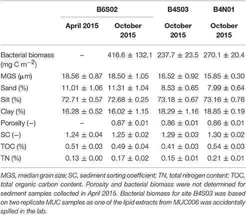
Table 2. Average (±SD) sediment-depth integrated (0-5 cm) environmental variables per site sampled in the GSR license area during GSRNOD15A (October 2015, all sites) and SO239 (April 2015, site B6S02).

FIGURE 2

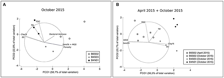
Figure 2. PCO plots of sediment-depth integrated (0–5 cm) environmental variables for all three sites sampled in the GSR license area (A) during GSRNOD15A (October 2015, all sites) and (B) during GSRNOD15A (October 2015, all sites) and SO239 (April 2015, site B6S02). MGS, median grain size; SC, sediment sorting coefficient; TN, total nitrogen content; TOC, total organic carbon content. Vectors represent sediment characteristics correlating >50% (based on Spearman correlation coefficients) with one of the two PCO axes. Note that in the second PCO analysis (B) sediment porosity and bacterial biomass were excluded from the analysis as these variables were not measured on samples collected in April 2015.

Intra-Annual Variability

At site B6S02, average daily NPP in April (271.2 g C m⁻² d⁻¹) exceeded that in October 2015 (214.7 g C m⁻² d⁻¹; see Figure 3). Moreover, the months prior to April 2015 (SO239) displayed the highest NPP values overall, whereas the months preceding GSRNOD15A were characterized by the lowest NPP. This difference in NPP between the two periods was not reflected in a dissimilarity in sediment characteristics [main PERMANOVA: Pseudo-F_{(1, 4)} = 0.55, P_MC = 0.64; see Table 2 and Figure 2B].

FIGURE 3

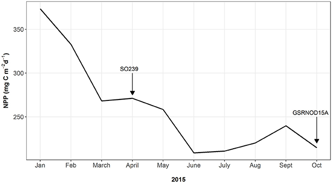
Figure 3. Monthly-averaged daily net primary productivity (NPP) for the surface water at site B6S02 for January–October 2015. Arrows indicate the timing of the SO239 cruise (April 2015) and that of the GSRNOD15A cruise (October 2015).

Meiofauna and Nematode Communities

Spatial Variability

Total meiofauna abundances in the top 0–5 cm of the sediment did not differ significantly between the three sites sampled during GSRNOD15A [main PERMANOVA: Pseudo-F_{(2, 5)} = 2.16, P_PERM = 0.22]. Nevertheless, on average, abundances declined from B6S02 (151.1 ± 54.2 ind. 10 cm⁻²) to B4S03 (106.6 ± 29.3 ind. 10 cm⁻²) and B4N01 (88.1 ± 55.0 ind. 10 cm⁻²). Meiofauna higher taxon composition differed significantly between sites according to the main PERMANOVA test [Pseudo-F_{(2, 6)} = 2.15, P_PERM = 0.03], but the pairwise tests could not identify pairwise differences (all P_MC > 0.05; see also Supplementary Figure 1A). Each site was dominated by the same taxa; nematodes prevailed (attaining relative abundances of 85.1–93.3% over all GSRNOD15A samples), followed by copepods (1.5–10.6%) and nauplii (1.1–7.1%; see Figure 4A). The other taxa encountered always contributed < 1% to total meiofauna abundance. Among-sample compositional differences were mainly driven by the less abundant taxa as the BVStep procedure selected Isopoda, Ostracoda, Polychaeta, and Tantulocarida as the subset best explaining the overall multivariate pattern (Rho = 0.69, P = 0.03). Moreover, these taxa were either restricted to (Isopoda restricted to B6S02) or (nearly) absent from one of the sites (Ostracoda and Tantulocarida absent from B4N01 and B6S02, respectively; Polychaeta only found in one B4N01 sample). None of the meiofauna taxon diversity indices computed differed significantly between the three sites (for all indices: main PERMANOVA: P_PERM > 0.05; Table 3).

FIGURE 4

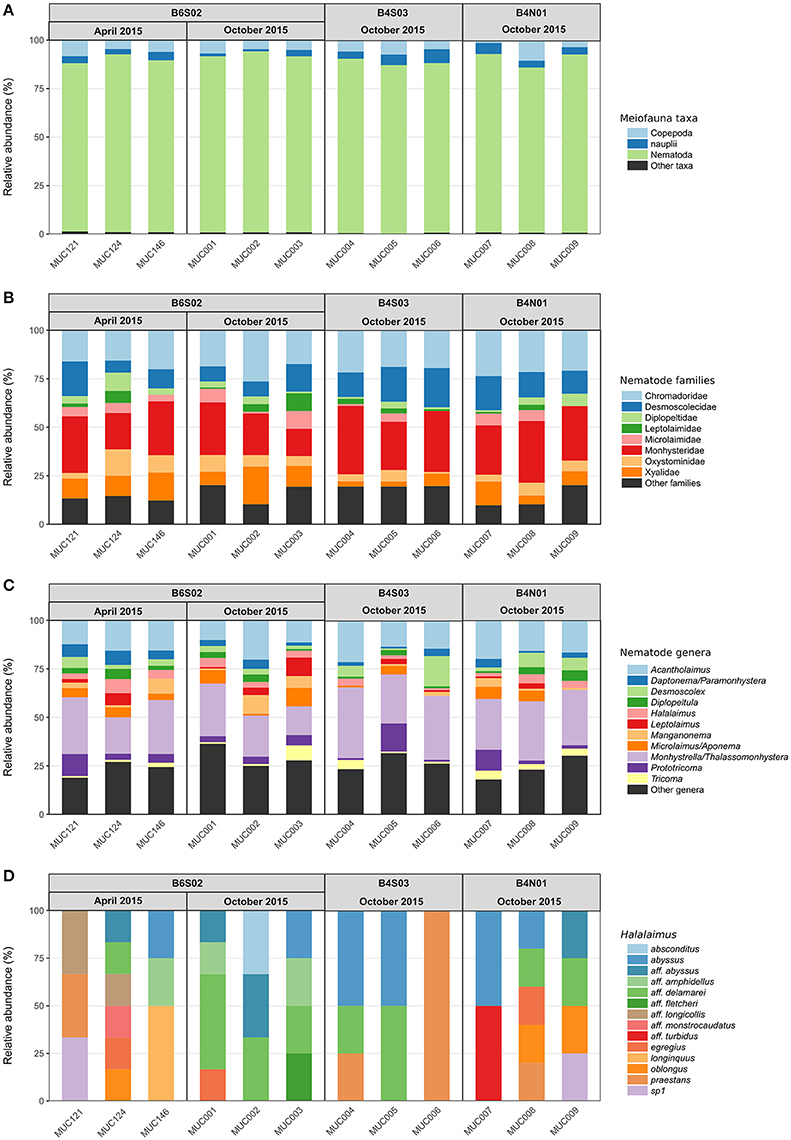
Figure 4. Relative abundances of (A) higher meiofauna taxa, (B) nematode families, (C) nematode genera, and (D) Halalaimus species per multicorer (MUC) sample for all sites sampled in the GSR license area during GSRNOD15A (October 2015, all sites) and SO239 (April 2015, site B6S02). “Other taxa” are higher meiofauna taxa that contributed <1% to total meiofauna abundance. “Other families” comprised <1% of the total number of nematodes identified per sample, and “other genera” comprised <5% of the total number of nematodes identified per sample.

TABLE 3

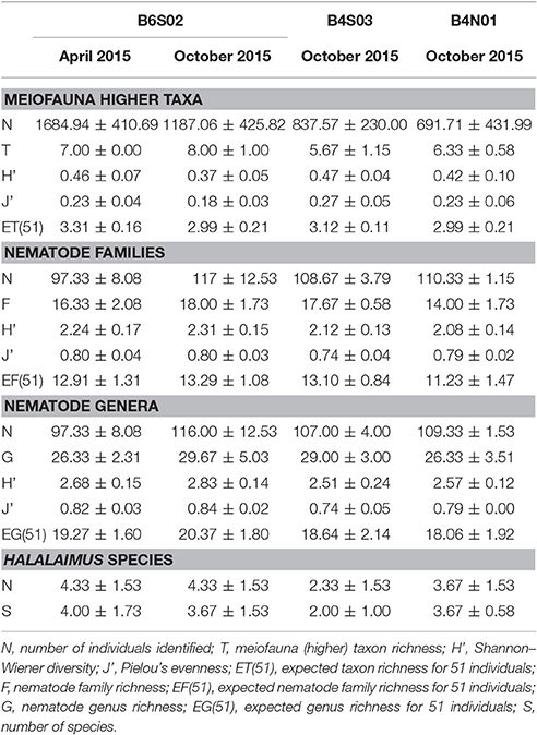
Table 3. Average (±SD) counts and values of diversity indices for meiofauna (higher) taxa, nematode families, nematode genera, and Halalaimus species per site sampled in the GSR license area during GSRNOD15A (October 2015, all sites) and SO239 (April 2015, site B6S02).

Nematode family composition (Figure 4B and Supplementary Figure 1B) showed no marked differences between sites [main PERMANOVA, Pseudo-F_{(2, 6)} = 1.21, P_PERM = 0.23], and more than half of the families were shared between sites (Supplementary Figure 2A). The prevailing families were Monhysteridae (26.9 ± 6.4%), Chromadoridae (21.1 ± 2.6%), and Desmoscolecidae (13.9 ± 4.6%), and together they comprised 47.4–72.6% of total nematode abundance. The PERMDISP test indicated a significantly different multivariate dispersion between sites [F_{(2, 6)} = 7.13, P_PERM = 0.03], caused by the lower dispersion for B4S03 (average dispersion: 11.63 ± 0.56%) relative to the other sites (B6S02: 15.47 ± 0.82%, B4N01: 15.89 ± 1.15%). Except for nematode family richness (F), there were no significant differences in family diversity indices between sites (main PERMANOVA: all P_PERM > 0.05). Pairwise PERMANOVA tests showed significantly fewer families at site B4N01 (14.00 ± 1.73) compared to B4S03 (17.7 ± 0.58; t = 3.48, P_MC = 0.03; Table 1). Although, average family richness at B6S02 (18 ± 1.73) also exceeded that at B4N01, the relatively high amongst-replicate variability for B6S02 resulted in a non-significant difference between B6S02 and B4N01 (t = 2.83, P_MC = 0.05). Although the main PERMANOVA test revealed a significant “site” effect on nematode genus composition [Pseudo-F_{(2, 6)} = 1.63, P_PERM = 0.02], the pairwise tests were unable to differentiate amongst pairs of sites (all P_MC > 0.05; see also Supplementary Figure 1C). As shown in Figure 4C, all three sites were dominated by the same set of nematode genera. Monhystrella/Thalassomonhystera (27.0 ± 6.4%) and Acantholaimus (15.9 ± 4.0%) dominated the nematofauna in all samples, except for MUC005 (B4S03) where Prototricoma was subdominant (14.4%). The subset of genera best explaining the among-sample compositional differences constituted 11 genera (BVStep: Rho = 0.90, P = 0.02), of which the majority was only present in few samples and mostly represented by one individual. Amongst these 11 genera were Diplopeltula, Manganonema, and Tricoma, which attained relatively high relative abundances in only a few samples (Figure 4C). More than 50% of the genera were restricted to one site (Supplementary Figure 2A). Site B6S02 was characterized by the highest nematode generic evenness (J′) [main PERMANOVA: Pseudo-F_{(2, 6)} = 6.83, P_PERM = 0.02; pairwise PERMANOVA: B6S02-B4N01, t = 3.92, P_MC = 0.02, B6S02-B4S03: t = 3.92, P_MC = 0.04]. The values of the other genus diversity indices were similar between the three sites (all P_PERM > 0.05). Figure 5A compares the values of three genus richness estimators (i.e., Bootstrap, Chao 1, and Jackknife2) between the three sites sampled during GSRNOD15A in function of the number of MUC deployments. Although G and expected genus richness [EG(51)] did not vary significantly between sites, the genus richness estimators calculated here were consistently lowest for site B4N01, intermediate for B4S03 and highest for B6S02.

FIGURE 5

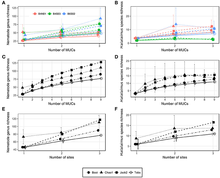
Figure 5. Nematode genus (A,C,E) and Halalaimus species (B,D,F) accumulation curves for (A,B) all MUCs taken per site, (C,D) all MUCs taken, and (E,F) all sites sampled during GSRNOD15A. Error bars denote standard deviations and are only provided for T_obs and Chao1 in the PRIMER v6 software. Boot, Bootstrap; Jack2, Jackknife 2; T_obs, observed taxon richness.

Figure 4D shows a highly variable Halalaimus species composition both within and between sites (see also Supplementary Figure 1D). Halalaimus abyssus (n = 6) and H. aff. delamarei (n = 9) were overall the most abundant; these were also the two only species shared between all sites (see also Supplementary Figure 2A). Half of the species was restricted to one site (see Supplementary Figure 2A). Halalaimus species richness and the values of all three species richness estimators, but also the number of Halalaimus individuals identified, were lowest for site B4S03 (see Table 3 and Figure 5B).

Intra-Annual Variability

At site B6S02, differences in total meiofauna abundance (0–5 cm) between April and October 2015 were statistically insignificant [main PERMANOVA, Pseudo-F_{(1, 3)} = 4.00, P_PERM = 0.11]. Nevertheless, average meiofauna abundances were higher in April (242.3 ± 59.2 ind 10 cm⁻²) than in October 2015 (151.1 ± 54.2 ind. 10 cm⁻²). The relative abundance of nematode juveniles did not change significantly between April (36.5 ± 8.2%) and October [37.8 ± 5.4%; main PERMANOVA, Pseudo-F_{(1, 4)} = 0.05, P_MC = 0.84]. Meiofauna higher taxon composition was comparable between April and October 2015 [main PERMANOVA: Pseudo-F_{(1, 4)} = 1.78, P_MC = 0.20], with nematodes being the dominant taxon (90.3 ± 2.3% over all B6S02 samples), and copepods (5.9 ± 1.4%) and nauplii (2.8 ± 1.2%) the second and third, respectively, most abundant groups (Figure 4A and Supplementary Figure 1A). Also meiofauna taxon diversity was comparable between April and October (all diversity indices: P_MC > 0.05). No differences could be discerned in nematode family [main PERMANOVA: Pseudo-F_{(1, 4)} = 0.61, P_MC = 0.67; Figure 4B and Supplementary Figure 1B] or genus composition [main PERMANOVA: Pseudo-F_{(1, 4)} = 1.11, P_MC = 0.38; Figure 4C and Supplementary Figure 1C] at site B6S02 between April and October 2015. All nematode family and genus diversity indices showed similar values for the two periods (main PERMANOVA, all P_MC > 0.05; see Table 3). Halalaimus species composition varied greatly within and between periods (see Figure 4D and Supplementary Figure 1D). Species richness was similar between April and October (Table 3). Although PERMANOVA tests failed to uncover an intra-annual change in meiofauna higher taxon, nematode family, and nematode genus composition, a considerable proportion of taxa was found only in samples from April or October (see Supplementary Figure 2). As shown by taxon accumulation curves in function of the number of periods sampled (data not shown), the investigation of site B6S02 during two different periods in 1 year resulted in, on average, 20% more meiofauna taxa, 10% more nematode families, 31% more nematode genera, and 44% more Halalaimus species compared to sampling only 1 period. The taxa that were restricted to one period were all rare, whilst the most abundant taxa were present in both periods.

Sampling Efficiency of Meiofauna and Nematode Diversity

Overall, 14 meiofauna taxa, 28 nematode families, 80 nematode genera, and 14 Halalaimus species were identified from the April and October 2015 samples collected in the GSR license area. Table 4 contains the observed number of taxa (T_obs) and the values of 3 taxon richness estimators (i.e., Chao1, Jack2, and boot) for meiofauna higher taxa, nematode families, nematode genera and Halalaimus species given the nine MUC samples collected during GSRNOD15A (October 2015). For meiofauna higher taxa, Chao1 could not be defined, as doubletons (i.e., taxa found twice) were absent. In October 2015, we encountered 14 higher meiofauna taxa, 28 nematode families, 77 nematode genera and 11 Halalaimus species within the GSR license area. Between 75.7 and 89.7% (based on sites), or between 76.5 and 91.5% (based on MUCs) of all meiofauna taxa present were found. For nematode families, the current sampling captured between 84.3 and 94.9% (sites) or between 87.8 and 94.9% (MUCs) of nematode family richness. For Halalaimus, it was estimated that 66.7–85.3% (sites) or 70.5–85.9% (MUCs) of the species present was sampled. In agreement, the Halalaimus species accumulation curves appeared to start leveling off (Figures 5D,F). Nematode genus richness was captured to the least extent by our sampling as between 65.5 and 85.7% (sites) and 60.4 and 85.6% (MUCs) of all genera were detected. The change in genus richness in function of the number of MUC samples (Figure 5C) and sites (Figure 5E) confirms the incomplete characterization of nematode genus richness, as none of the curves reach an asymptote. Based on Chao1, we need 1 (or 1.1 times the current sampling effort) or 12 additional samples (or 2.3 times the current sampling effort) to characterize 95 or 100%, respectively, of total nematode family richness. To characterize 95 and 100% of total nematode genus richness, an extra 22 (3.4 times the current sampling effort) or 72 (9 times the current sampling effort) MUC samples, respectively, are required. For Halalaimus, 8 (2 times the current sampling effort) or 19 (3 times the current sampling effort) additional samples are needed to capture 95 or 100% of total species richness within this genus.

TABLE 4

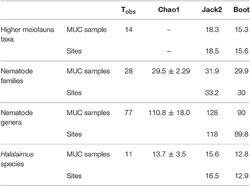
Table 4. Observed (T_obs) and estimated taxon richness for higher meiofauna taxa, nematode families, nematode genera, and Halalaimus species based on the accumulation of GSRNOD15A MUC samples (n = 9) and sites (n = 3).

Discussion

Spatial Variability in Meiofauna and Nematode Communities within the GSR License Area

Despite the large geographical distances (60–270 km) and the statistically significant (albeit small) differences in sediment granulometry between the three nodule-bearing sites sampled in the GSR license area, the abundance, composition and diversity of meiofauna and nematode communities were largely comparable. This resemblance in abyssal meiobenthic communities between sites located around 60 km apart is presumably related to the largely similar environmental setting, with all sites constituting the same macro-habitat (cfr. Vanreusel et al., 2010) being equally deep nodule-bearing deep-sea silts. Similarly, geographically disparate, isobathic sites in various nodule-free deep-sea regions were shown to harbor similar meiofauna and nematode communities, at least as long as sediment granulometry and food availability were comparable (e.g., Lambshead et al., 2003; Sebastian et al., 2007; Pape et al., 2013; Lins et al., in press).

Several studies documented an effect of taxonomic resolution on spatial patterns in deep-sea benthic communities (Narayanaswamy et al., 2003; Muthumbi et al., 2011; Lins et al., in press). In the GSR license area, both the meiofauna (this study) and macrofauna (De Smet et al., 2017; this issue) were spatially homogenous irrespective of the taxonomical level considered. However, lower-level taxonomical identifications (family, genus, or species) were in both investigations restricted to particular taxa (this study: Nematoda; De Smet et al., 2017: Isopoda and Polychaeta). To make accurate inferences about the taxonomic resolution required to detect macro-ecological patterns in benthic size groups, more taxa need to be identified down to lower taxonomical level.

Although, overall no large spatial variability was observed in terms of sediment environmental variables and meiobenthic communities within the GSR license area, there were some subtle differences between sites in terms of specific meiofauna and nematode community attributes and environmental variables. First of all, there was a (non-significant) tendency of site B6S02 having higher sedimentary bacterial biomass, meiofauna abundances, and total estimated nematode genus richness relative to the other two sites sampled. This finding may be ascribed to the higher food availability at B6S02, inferred from seafloor POC flux calculated according to Lutz et al. (2007) [i.e., B6S02 (1.61 g C_org m⁻² yr⁻¹) > B4S03 (1.56 g C_org m⁻² yr⁻¹) > B4N01 (1.51 g C_org m⁻² yr⁻¹)]. In agreement, higher benthic bacterial biomass (Smith et al., 1997) and meiofauna abundances (Smith et al., 2008) have been linked before to elevated POC flux rates to the seabed in the CCFZ. Both polychaete (Glover et al., 2002; Wilson, 2016) and nematode species (Lambshead et al., 2003) diversity showed a positive relationship with seafloor POC flux for a variety of sites in the Eastern Tropical Pacific, including the CCFZ, though these studies covered a wider range of productivity. Likewise, De Smet et al. (2017), who sampled the same three sites in the GSR license area, recorded the highest polychaete (family) diversity at site B6S02. The rather small POC flux gradient covered here may explain the absence of statistically significant results. Secondly, even though the meiofauna and nematode communities at the three sites were dominated by the same taxa, there were some minor compositional differences owing to the less abundant or rare taxa, of which most had a seemingly limited spatial distribution (although this may simply be an artifact of under-sampling). Spatial distribution patterns of dominant and rare meiofauna taxa did not concur in the few nodule-free deep-sea systems investigated (Bianchelli et al., 2008; Gambi et al., 2010), suggesting these are driven by different processes. Several theories exist to explain patterns in taxon richness and coexistence (Holt, 2003; Leibold et al., 2004), but the mechanisms underlying these in the deep sea are still not fully understood (Gage, 1996; Gray, 2002; McClain and Hardy, 2010).

Intra-Annual Variability in Meiofauna and Nematode Communities

In oligotrophic deep-sea areas, like the CCFZ, biological responses to seasonally fluctuating organic matter input are generally restricted to bacteria and protozoans (Gooday, 2002). This may explain the lack of significant intra-annual variability in metazoan meiofauna (higher taxon level) and nematode (families and genera) abundance, composition and diversity observed at site B6S02 in the GSR license area. Nevertheless, interannual differences in nematode abundance (Miljutin et al., 2015), nematode genus composition (Radziejewska et al., 2001; Miljutin et al., 2015) and nematode genus diversity (Miljutin et al., 2015) observed in the CCFZ, were thought to be driven by interannual differences in primary productivity and the resultant flux of organic matter to the seabed. Possibly, the magnitude of the temporal difference in primary productivity observed here was not large enough to elicit a response by the meio- and nemato-fauna. Miljutin et al. (2015) mentions a difference in surface productivity (in terms of surface water chlorophyll a concentration) of a factor 1.6 between the 2 years the IFREMER area was investigated, which is slightly higher than that observed here (1.3). However, even in the Southern Ocean where the effect of an eight-fold difference in productivity was examined, no significant change in meiofauna standing stock was noted (Veit-Köhler et al., 2011). Alternatively, the meiofauna and nematode community may have reacted to the seasonally varying input of organic matter by changing vertical distribution (Veit-Köhler et al., 2011) or biomass, both of which were not assessed here.

Sampling Efficiency of Meiofauna and Nematode Diversity

The foregoing shows that the present sampling strategy allowed for the detection of macro-ecological patterns, but the question remains whether it adequately captured meiofauna and nematode diversity. Our study potentially characterized more than 90% of meiofauna taxa and nematode families present in the GSR license area, but comparatively more samples are needed to characterize the majority of the nematofauna at a genus level and the nematode genus Halalaimus at the species level. To accurately assess the level of biodiversity, it is crucial to work at the highest taxonomic resolution possible, i.e., species level (as recommended by ISA, 2015). The morphological identification of deep-sea nematodes, especially to species level, is time-consuming and difficult owing to the high number of undescribed species and, specifically for abyssal nodule areas, the dominance of speciose genera like Thalassomonhystera and Acantholaimus (Miljutina et al., 2010; Miljutin and Miljutina, 2016). Moreover, differences in diagnostic characteristics between different genera are not always unambiguous (Miljutina et al., 2010), which is why several genera were grouped here. As a consequence, the only species-level studies conducted in the CCFZ assigned nematodes to morphospecies (Lambshead et al., 2003; Miljutina et al., 2010), leaving these datasets incomparable and therefore hampering a region-wide assessment of biodiversity and connectivity. Furthermore, traditional morphological biodiversity assessment does not allow for the detection of cryptic species (Bhadury et al., 2008), which may be common amongst deep-sea nematodes including those inhabiting the CCFZ (Smith et al., 2008). A promising technique for rapid biodiversity analysis is metabarcoding of environmental samples (Taberlet et al., 2012; Fonseca et al., 2014), although currently it cannot yet serve as a tool to reliably and accurately estimate (deep-sea) nematode diversity (Porazinska et al., 2009; Dell'Anno et al., 2015). One of the biggest problems with employing this approach for deep-sea nematodes is the lack of an adequate reference database (Dell'Anno et al., 2015; Sinniger et al., 2016). Hence, combined morphological and molecular biodiversity assessment is still warranted (Sinniger et al., 2016).

Based on the Chao 1 estimator, to capture 95 or 100% of the nematode genera present in the GSR license area, sampling effort would need to increase three- to nine-fold, respectively. As the full characterization of nematode genus richness required more samples than that of family richness, it is expected that even more samples are needed to adequately assess total nematode species richness. However, in agreement with Wilson (2016), the collection and processing of this estimated total number of samples required to capture meiobenthic diversity (nearly) fully, is highly impractical. In practice, the level of sampling effort should be a compromise between practical feasibility and the degree of coverage of total biodiversity (e.g., 90% of the total number of species present). The latter can be estimated through the extrapolation of taxon accumulation curves with taxon richness estimators, as was done in the present study. However, the minimal fraction of biodiversity to be covered or the minimal sampling effort in environmental baseline studies (and later on, in monitoring studies) in the CCFZ has so far not been stipulated by the International Seabed Authority (ISA), the regulator for the exploration for deep-sea mining in the Area Beyond National Jurisdiction (ISA, 2012; Durden et al., 2016).

Comparison with Other Abyssal (Nodule-Bearing) Site Studies

There are considerable discrepancies amongst this and previous studies on meiofaunal ecology in abyssal nodule areas in terms of sampling methodology, location, and timing (see Supplementary Table 1 and Supplementary Figure 3). This greatly complicates the comparison of meiofauna and nematode community descriptors between studies. Nevertheless, despite these aforementioned differences in sampling strategies, meiofauna densities documented for the GSR license area were broadly similar to those reported for other nodule-bearing abyssal sediments, including the CCFZ (Supplementary Figure 4).

As generally observed for deep-sea sediments world-wide (e.g., Lampadariou and Tselepides, 2006; Shimanaga et al., 2007; Veit-Köhler et al., 2011) including (CCFZ) nodule-bearing sediments (Snider et al., 1984; Renaud-Mornant and Gourbault, 1990; Shirayama, 1999; Ahnert and Schriever, 2001; Mahatma, 2009), the meiofauna in the GSR license area was dominated by nematodes (>85%). The predominant nematode families (i.e., Monhysteridae, Chromadoridae, and Desmoscolecidae) and genera (i.e., Monhystrella/Thalassomonhystera and Acantholaimus) in the GSR license area also attain high relative abundances in other nodule-bearing sites in the CCFZ (Renaud-Mornant and Gourbault, 1990; Lambshead et al., 2003; Miljutina et al., 2010) and other basins (Vopel and Thiel, 2001; Singh et al., 2014), as well as in nodule-free CCFZ sediments (Radziejewska et al., 2001). Moreover, these taxa are common in nodule-free abyssal sediments from around the World Ocean too (Miljutina et al., 2010; Vanreusel et al., 2010; Singh et al., 2016). Note, however, that subtle differences exist in the order of dominance of nematode taxa in abyssal nodule-bearing sediments, which may reflect spatial and/or temporal patterns or which may simply be a consequence of the different sediment depth strata sampled (see Supplementary Table 1). Six out of the fourteen Halalaimus species identified from the GSR license area were described for the first time from a nodule-bearing site in the Peru Basin (Bussau, 1993). Amongst those six species is H. egregius which was also reported for the eastern IFREMER license area (see Supplementary Figure 3) west off the GSR area (Miljutina et al., 2010). Thus, morphological data suggest potential connectivity between the GSR and the IFREMER license area in the CCFZ (100s of kilometers apart), and between these two CCFZ areas and the Peru Basin (1,000s of kilometers apart). However, molecular data are needed to confirm whether these are in fact the same species or whether they constitute cryptic species. Apparently, the degree of cryptic speciation in CCFZ nematodes is considered to be substantial (Smith et al., 2008).

In conclusion, it seems that the same suite of meiofauna and nematode taxa prevail (although in differing orders of dominance) in nodule-bearing (and nodule-free) sediments sampled within license areas (at a spatial scale of 10s–100s km), in different CCFZ license areas (100s–1,000s km) and in different regions (1,000s–10,000s km). These dominant taxa also occur in other deep-sea macro-habitats (though, again, not necessarily with the same proportions), supporting the notion of a low level of endemism for meiofauna taxa and nematode genera in the deep sea (Bik et al., 2010, 2012; Zeppilli et al., 2011). The fact that geographically disparate nodule-bearing CCFZ license areas and abyssal regions share potentially the same Halalaimus species, implies that a wide distribution range may not be limited to higher taxonomical levels. The existence of wide-spread deep-sea nematode species has already been reported based on morphological data (Miljutin et al., 2010). Moreover, identical ribosomal sequences, potentially representing the same species, were retrieved from sites separated by more than 10,000 km for taxa belonging to the Enoplida, an order to which also Halalaimus belongs (Bik et al., 2010).

Implications for Environmental Management and Suggestions for Future Research

The present findings indicate that distant, equally deep nodule-bearing sediments within the GSR license area are inhabited by similar meiofauna communities, and that the dominant taxa also occur in remote nodule-bearing and nodule-free deep-sea localities. Thus, based on water depth and nodule presence, different macro-habitats, with each habitat expected to harbor similar meiofaunal communities, can be delineated through habitat mapping (Lamarche et al., 2016). Together with similar data on other benthic size groups (macro- and mega-fauna), the current meiofaunal data will aid the spatial planning of PRZs and IRZs in the GSR license area. Given that intra-annual variability in meiofaunal composition, standing stock, and diversity might be limited, any temporal changes observed in these community attributes during the monitoring of mined sites will most probably be directly resulting from mining activities. Any potential mining-induced alterations in meiofaunal communities may then be mitigated by recolonization from these PRZs, given that these are within the range of the maximal dispersal distance. Nonetheless, it is important to note that species-level, and preferably molecular, data are needed to confirm these acclaimed broad distribution ranges of meiofauna taxa and high connectivity between different deep-sea sites. Moreover, more research is needed on the influence of habitat heterogeneity, driven by spatial variability in, for instance, topography, nodule abundance and nodule size, on meiofaunal communities to ascertain the suitability of candidate preservation zones. Understanding the mechanisms responsible for taxon distributions, will help to gauge the extinction risks and recovery rates of taxa. Finally, the high proportion and the significant contribution to spatial variability in community composition of rare meiofauna and nematode taxa in the GSR license area, together with their potentially elevated extinction risk, warrant closer scrutiny of their functional importance. In highly diverse systems, like the deep sea, the presence of many rare taxa may act as a buffer against taxon loss following e.g., environmental disturbances (Naeem, 1998). In highly diverse terrestrial and coastal ecosystems, rare taxa have been shown to possess unique functional traits (Mouillot et al., 2013). For (nodule-bearing) deep-sea systems, however, information on the functional importance of rare taxa is lacking.

Author Contributions

Conceived and designed the sampling design: EP, AV. Performed the sampling: EP, FH. Processed the samples: EP, TB. Analyzed the data: EP. Wrote the paper: EP, AV. Critically reviewed the paper: FH, TB.

Funding

The SO239 cruise with the RV Sonne was financed by the German Ministry of Education and Science BMBF as a contribution to the European project JPI-Oceans “Ecological Aspects of Deep-Sea Mining.” The first author was funded by a service agreement between Ghent University and Global Sea Mineral Resources (GSR). The second author received funding from the service agreement between Ghent University and GSR, and from the Department of Economy, Science & Innovation of Flanders under the framework of JPI-Oceans.

Conflict of Interest Statement

The authors declare that the research was conducted in the absence of any commercial or financial relationships that could be construed as a potential conflict of interest.

The handling Editor declared a past collaboration with some of the authors, and the handling Editor states that the process nevertheless met the standards of a fair and objective review.

Acknowledgments

We are greatly indebted to the captain and crew on the sampling expeditions with the RV Sonne (SO239) and RV Mt. Mitchell (GSRNOD15A) for assistance with sampling. A special thanks goes out to François Charlet (exploration manager) and Tom De Wachter (environmental manager) from GSR, Alison Proctor, Phil Wass and Tony Wass from Ocean Floor Geophysics, Nick Eloot and Karen Soenen from G-TEC, and Carmen Juan, Niels Viaene, and Liesbet Colson from Ghent University. Dirk Van Gansbeke, Bart Beuselinck, Niels Viaene, and Annick Van Kenhove are acknowledged for aiding with sample analyses. Dan Jones kindly provided gridded global seafloor POC flux data.

Supplementary Material

The Supplementary Material for this article can be found online at: http://journal.frontiersin.org/article/10.3389/fmars.2017.00205/full#supplementary-material

Footnotes

1. ^InterOceanMetal, consortium of Bulgaria, Cuba, Czech Republic, Poland, Russian Federation, and Slovakia.

2. ^Institut Français de Recherche pour l'Exploitation de la MER, France.

3. ^Deep Ocean Resources Development company, Japan.

4. ^Cook Islands Investment Corporation, Cook Islands.

References

Ahnert, A., and Schriever, G. (2001). Response of abyssal Copepoda Harpacticoida (Crustacea) and other meiobenthos to an artificial disturbance and its bearing on future mining for polymetallic nodules. Deep Sea Res. II Top. Stud. Oceanogr. 48, 3779–3794. doi: 10.1016/S0967-0645(01)00067-4