 Benjamin A. Lange1,2*†
 Christian Katlein1
 Giulia Castellani1
 Mar Fernández-Méndez1,3
 Marcel Nicolaus1
 Ilka Peeken1,4
 Hauke Flores1,2
- 1Alfred-Wegener-Institute Helmholtz Center for Polar and Marine Research, Bremerhaven, Germany
- 2Centre for Natural History (CeNak), Zoological Museum, University of Hamburg, Hamburg, Germany
- 3Norwegian Polar Institute, Fram Centre, Tromsø, Norway
- 4MARUM, Center for Marine Environmental Sciences, University of Bremen, Bremen, Germany
Assessing the role of sea ice algal biomass and primary production for polar ecosystems remains challenging due to the strong spatio-temporal variability of sea ice algae. Therefore, the spatial representativeness of sea ice algal biomass and primary production sampling remains a key issue in large-scale models and climate change predictions of polar ecosystems. To address this issue, we presented two novel approaches to up-scale ice algal chl a biomass and net primary production (NPP) estimates based on profiles covering distances of 100 to 1,000 s of meters. This was accomplished by combining ice core-based methods with horizontal under-ice spectral radiation profiling conducted in the central Arctic Ocean during summer 2012. We conducted a multi-scale comparison of ice-core based ice algal chl a biomass with two profiling platforms: a remotely operated vehicle and surface and under ice trawl (SUIT). NPP estimates were compared between ice cores and remotely operated vehicle surveys. Our results showed that ice core-based estimates of ice algal chl a biomass and NPP do not representatively capture the spatial variability compared to the remotely operated vehicle-based estimates, implying considerable uncertainties for pan-Arctic estimates based on ice core observations alone. Grouping sea ice cores based on region or ice type improved the representativeness. With only a small sample size, however, a high risk of obtaining non-representative estimates remains. Sea ice algal chl a biomass estimates based on the dominant ice class alone showed a better agreement between ice core and remotely operated vehicle estimates. Grouping ice core measurements yielded no improvement in NPP estimates, highlighting the importance of accounting for the spatial variability of both the chl a biomass and bottom-ice light in order to get representative estimates. Profile-based measurements of ice algae chl a biomass identified sea ice ridges as an underappreciated component of the Arctic ecosystem because chl a biomass was significantly greater in this unique habitat. Sea ice ridges are not easily captured with ice coring methods and thus require more attention in future studies. Based on our results, we provide recommendations for designing an efficient and effective sea ice algal sampling program for the summer season.
Introduction
There is mounting evidence for an overall increase in Arctic-wide net primary production (NPP) as a result of the declining sea ice cover and increasing duration of the phytoplankton growth season (Arrigo and van Dijken, 2011, 2015; Fernández-Méndez et al., 2015). However, it remains uncertain how sea ice algae NPP will respond to continued changes of the sea ice environment. It has been suggested that a thinning Arctic sea ice cover, which will lead to increased light transmittance, will also result in increased sea ice algal NPP rates due to more available photosynthetically active radiation (PAR; Nicolaus et al., 2012; Fernández-Méndez et al., 2015). On the other hand, some forecasts predict increased snow precipitation in the Arctic (IPCC, 2013), which would result in less available light for bottom-ice algal growth during spring. Other than available light, other variables may have an equal or greater influence on Arctic primary production depending on region and season. Such variables include nutrient supply, temperature, and CO2 intake (Tremblay et al., 2015). Declining sea ice may increase oceanic CO2 intake, which would result in increased NPP, but could be counteracted by increased runoff and higher temperatures expected throughout the Arctic (Tremblay et al., 2015).
In the central Arctic Ocean sea-ice algae has been documented to contribute up to 60% of the NPP during summer (Gosselin et al., 1997; Fernández-Méndez et al., 2015). However, net sympagic (ice-associated) primary production is relatively low accounting for 1–10% of total NPP in the Arctic Ocean (Dupont, 2012; Arrigo and van Dijken, 2015). Regardless of the overall low contribution of sympagic NPP, both sympagic and pelagic organisms showed a high dependency on ice-algae produced carbon within the central Arctic Ocean (Budge et al., 2008; Wang et al., 2015; Kohlbach et al., 2016, 2017). The key role of sea ice algae in Arctic foodwebs, particularly in terms of reproduction and growth of key Arctic organisms, such as: Calanus glacialis (Michel et al., 1996; Søreide et al., 2010), highlights the importance of timing and duration of ice algal growth, and the availability of algal biomass throughout different times of the year.
Spatial variability of springtime ice algal chl a biomass has been related to the distribution of snow on first-year sea ice (FYI), due to the large influence of snow on light transmission by the reflection and scattering of light near the surface. This relationship explains the similar patch sizes observed for snow and sea ice algae biomass on the same study sites. Between study sites, however, patch sizes had a large range between 5 and 90 m, which was the result of differences in the snow distribution and drifting patterns over relatively level FYI (Gosselin et al., 1986; Rysgaard et al., 2001; Granskog et al., 2005; Søgaard et al., 2010). In contrast, the undulating surface topography of MYI plays an important role in the distribution of snow, which has been linked to the presence of high ice algal chl a biomass at the bottom of thick MYI hummocks with little or no snow cover (Lange et al., 2015, 2017). Gradinger et al. (2010) identified sea ice ridges as important accumulation regions of sea ice fauna during advanced melt. This further highlights the ecological importance of thick sea ice features. Using traditional coring methods, however, it is very difficult to sample ridges and hummocks resulting in sparse observations for ice algae at the bottom or within these features.
In summer when the snow is melted and melt ponds are present, light availability has a less important role in controlling the distribution of ice algal chl a biomass. This is due to increased melt induced algal losses during late-spring and early-summer, which becomes the limiting factor controlling the ability of algal communities to remain in the bottom-ice environment (Grossi et al., 1987; Lavoie et al., 2005). The spatial distribution of ice algal chl a biomass during mid- to late-summer, however, remains poorly understood and under-sampled, particularly in the central Arctic Ocean (Wassmann et al., 2011; Miller et al., 2015).
The high spatial and temporal variability of sea ice algae, in addition to sparse sampling, results in poorly constrained sea ice algal chl a biomass and PP estimates for the central Arctic Ocean (Miller et al., 2015). Large-scale estimates of sea ice algal chl a biomass and PP are limited to modeling studies as satellites are unable to observe the underside of sea ice. Lee et al. (2015) demonstrated that pelagic phytoplankton PP models for the Arctic Ocean were highly sensitive to uncertainties in chlorophyll a (chl a) and performed best with in situ chl a data. In situ ice algal chl a estimates used in models, however, are typically based on a small number of ice core observations (e.g., Fernández-Méndez et al., 2015). A recent study comparing ice core chl a biomass to sea ice algal chl a biomass derived from an 85 m ROV transect of under-ice spectral radiation measurements showed large differences, which could carry high uncertainties for large-scale estimates based on these ice core data alone (Lange et al., 2016).
Miller et al. (2015) reviewed the different methods for PP measurements with spatial sampling resolution on the order of 0.01 m for ice coring-based in vitro incubations (e.g., Gosselin et al., 1997; Gradinger, 2009; Fernández-Méndez et al., 2015) or in situ incubations (e.g., Mock and Gradinger, 1999; Gradinger, 2009). At larger scales the under-ice eddy covariance method integrates primary production over an area of 100 m2 (Long et al., 2012). Thus there is a large gap in spatial coverage between the 0.01 to 100 m2 scales, which is not resolved by these methods. It is within this spatial range that many sea ice and snow properties (such as thickness, porosity, temperature) can vary, which can have a large influence on light availability, ice melt and growth, nutrient availability, and therefore, the spatial distribution of ice algae. Typical patch sizes of snow have been reported in the range 20–25 m (Gosselin et al., 1986; Steffens et al., 2006). Surface properties such as albedo have patch sizes of ~10 m (Perovich et al., 1998; Katlein et al., 2015a) and sea ice draft can vary at scales of around 15 m (Katlein et al., 2015a).
Here we present a novel approach to fill this important gap in the spatial scales of ice algal chl a biomass and NPP estimates by combining in vitro photosynthetic parameters of ice algae with chl a biomass derived from under-ice spectral radiation measurements and under-ice available PAR measurements obtained from a moving under-ice profiling platform, the ROV. Furthermore, we investigate the spatial patterns of chl a biomass and NPP estimates, using two under-ice profiling platforms: the ROV and Surface and Under Ice Trawl (SUIT), with special emphasis on sea ice ridges, and evaluate potential discrepancies between the up-scaled and ice core-based estimates. Based on our results, we provide recommendations for designing an efficient and effective sea ice algal sampling program for the summer season.
Materials and Methods
The Profiling Platforms
All surveys were conducted during the RV Polarstern expedition PS80 to the central Arctic Ocean in August and September 2012. Under-ice profiling platform surveys were conducted using an under-ice Remotely Operated Vehicle (ROV) V8Sii-ROV (Ocean Modules, Åtvidaberg, Sweden) and a SUIT (van Franeker et al., 2009), with mounted sensor arrays, described in Nicolaus and Katlein (2013), David et al. (2015), and Lange et al. (2016). Simplified diagrams and images showing the deployment of the under-ice profiling platforms were presented in Lange et al. (2016). The ROV is an under-water vehicle with mounted sensor array deployed through a small 2 × 2 m man made hole in the sea ice, and is attached by a 300 m long fiber optic cable. The ROV is controlled remotely from a sheltered base station (e.g., tent) located adjacent to the deployment hole. A detailed description of the ROV spectral measurements, calibration and calculations, and ROV operation was provided by Katlein et al. (2015b) and Nicolaus and Katlein (2013). The V8ii ROV was equipped with an altimeter (DST Micron Echosounder, Tritech, UK), a sonar (Micron DST MK2, Tritech, UK), one zoom-camera (Typhoon, Tritech, UK), and one fixed focal length camera (Ospray, Tritech, UK). The SUIT is a net developed for deployment in ice covered waters, typically behind an icebreaker, for sampling sea ice associated zooplankton and micronekton in the upper 2 m of the water within the ice-water interface. During this cruise the sensor array was specifically enhanced to measure the variability of sea ice algae chl a biomass within the sea ice and sea ice habitat properties along the SUIT hauls. The new sensor package included an Aquadopp Acoustic Doppler Current Profiler (ADCP; Nortek AS, Rud, Norway), a Conductivity Temperature Depth probe (CTD; Sea and Sun Technology, Trappenkamp, Germany) with a built-in Cyclops 7 fluorometer (Turner Designs, Sunnyvale, CA, USA), an PA500/6S altimeter (Tritech International Ltd., Aberdeen, UK), one RAMSES-ACC irradiance sensor (Trios, GmbH, Rastede, Germany), one RAMSES-ARC radiance sensor (Trios GmbH, Rastede, Germany) and a forward-looking video camera (GoPro Hero 2).
The ROV spectral surveys were conducted during seven ice stations (Table 1; Figure 1). The SUIT spectral surveys were conducted at 6 stations (Table 1; Figure 1). Stations conducted in relatively close proximity (< 50 km) to each other were grouped into similar locations represented by the letters A to I (Figure 1). Two profiles separated by small distances were sampled using the SUIT (< 10 km) at location B, and using the ROV (< 500 m) at locations C and D. Incoming solar radiation observations were measured on-ice for ROV-based spectral measurements, and from a ship-mounted sensor for SUIT-based spectral measurements. To ensure high quality spectra, data were limited to observations at a distance to the ice-bottom of ≤ 1 m and with a pitch and roll between −10° and 10°, as suggested by Nicolaus and Katlein (2013) and Katlein et al. (2016). Reducing the pitch and roll, and distance to ice bottom also reduced the potential influence of spectral absorption by the water. Since the SUIT behaves less predictable near ridges (e.g., it hits the ridge and is redirected in an unpredictable direction), we manually inspected the spectra to identify reliable spectral measurements at sea ice ridges (e.g., noisy spectra). Less than 1% of the spectra were excluded from analyses.
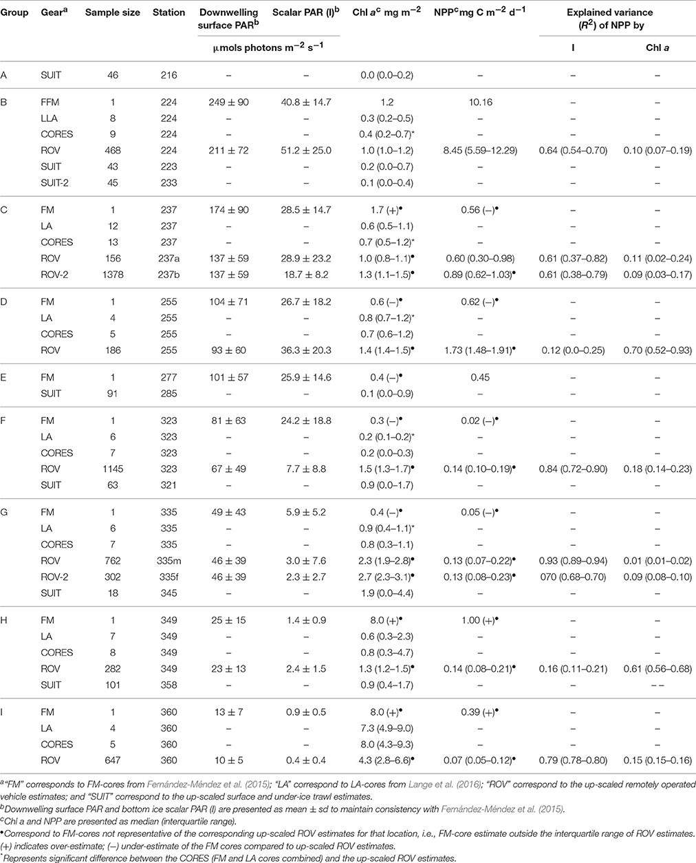
Table 1. Summary of downwelling surface and bottom-ice light, chlorophyll a biomass (chl a), net primary production (NPP), and explained variance of NPP per location (shown in Figure 1) and sampling method (gear): ice cores (FM or LA), remotely operated vehicle (ROV) and surface and under-ice trawl (SUIT).
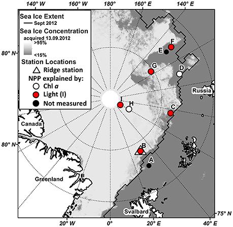
Figure 1. Map of the Arctic Ocean with sea ice extent and concentration data, and the locations of the corresponding station groupings conducted during the 2012 PS80 cruise (station numbers for each grouping are listed in Table 1). Locations are color coded to identify which variable, light (red) or chl a biomass (white), explains the dominant portion of the net primary production variance. The ice station with identified ridges, station 224 (location B), is identified by a triangle. Sea ice concentration data acquired from www.meereisportal.de according to algorithms in Spreen et al. (2008). Sea ice extent correspond to the 2012 September monthly mean (extent data acquired from NSIDC, (Fetterer et al., 2002, updated 2011).
Sea ice draft was calculated based on sensor measurements of depth and distance to ice bottom, and corrected for pitch and roll angles as described in Lange et al. (2016) and David et al. (2015). Sea ice ridges were identified from the SUIT ice draft profiles using the Rayleigh criteria, following procedures described by Rabenstein et al. (2010) and Castellani et al. (2014) for the sea ice surface topography, and Castellani et al. (2015) for the sea ice bottom profile. Ice draft local minima (thicker sea ice draft values are more negative) identified along the SUIT profiles with a threshold of 1.5 m deeper than the surrounding ice, following Castellani et al. (2015), were selected as potential ridges. Adjacent minima needed a separation distance between points which was less than half the depth of the first minima in order to be identified as two single elements not belonging to the same ridge. Ridge depth and width were measured in order to calculate ridge density (ridges km−1) and percent coverage of ridges. Here, ridge depth was calculated as the width at half maximum. During one SUIT haul (station 358, location H) there were no altimeter measurements. Because the SUIT generally travels directly under the ice, the depth measurements can be used to reliably (R2 = 0.78) derive level ice draft using a simple linear model (David et al., 2015). We could calculate ridge density, ridge coverage, and ridge width from these ice draft measurements without altimeter data. The absolute draft values at ridges, however, were less accurate and therefore excluded from analysis.
All profiling platform-derived observations (i.e., transmittance, sea ice algal chl a, NPP, draft) were divided into 5 ice classes based on the sea ice draft values in the following ranges: (1) 0–0.5 m; (2) 0.5–1.0 m; (3) 1.0–1.5 m; (4) 1.5–2.0 m; and (5) >2.0 m. Furthermore, we separated profiling platform-derived observations into level ice and ridged ice. This was done by manually identifying all observations acquired under the identified ridges. We identified dominant ice classes for each location using the modal ice thickness (converted to draft by multiplying by 0.9) from electromagnetic induction sounding ice thickness surveys, using an EM31 instrument, of the entire floe (data presented in Boetius et al., 2013; Fernández-Méndez et al., 2015; Katlein et al., 2015b). We used these larger scale ice thickness surveys to assign the dominant ice class because these surveys were conducted specifically for the purpose of assessing the distribution of ice thickness at the ice floe. Ground-based EM surveys are a common method to representatively capture the spatial variability of ice thickness on floe scales (Haas et al., 1997; Haas, 2004).
Sea Ice Algal Chl a Biomass Estimates Derived from Under-Ice Spectral Radiation
Ice algal chl a biomass estimates were derived from under-ice profiling platform-based spectral transmittance observations using empirical orthogonal function (EOF) analysis combined with generalized linear models (GLM), as described in Lange et al. (2016). EOF analyses reduce the dimensionality of the data while maintaining the variability of key spectral absorption properties, which can then be used to relate to chl a concentrations or other environmental variables. GLMs were fitted using ice core chl a concentrations as a response variable and EOF modes as predictor variables. All ice cores were extracted along ROV spectral radiation profiles. The best set of EOF modes used as predictor variables was selected by searching all possible combinations of EOF modes and using the Bayesian Information Criterion (BIC) to assess the quality of the GLM. The EOFs used represented the spectral variability that can best be explained by the variability within the ice algal chl a biomass. Furthermore, EOF analyses captured variability within multiple regions of the PAR light spectrum (400–700 nm) where chl a light absorption occurs. In addition, we used mean robustness R2 and true prediction error estimates as ranking criteria to find the best predictive model for our data set. Each model was applied to 5 data subsets not used to fit the model then we determined the predicted vs. observed R2-value for each data subset then took the mean R2-value as the mean robustness R2. To determine the true prediction error estimate we used 10-Fold Cross-Validation (10 FCV). In 10 FCV, data are randomly separated into 10 data subsets then model fitting and error estimation are repeated 10 times. Each time the model is fitted to 9-folds then applied to the 10th-fold. This is repeated 100 times and the mean of all root mean square error (RMSE) values is used as the true prediction error estimate. Based on these criteria we determined that the combination of spectral transmittance, calculated according to Nicolaus et al. (2010), and the EOF approach resulted in the most reliable predictive model (EOF-Transmittance) with a predicted vs. observed chl a R2 of 0.90, and a true prediction error estimate (10-fold cross validated root mean squared error, RMSECV), of 1.8 mg chl a m−2 (model M15 from Lange et al., 2016). In addition, the selected predictive model showed good agreement between chl a estimates derived from independent spectral data (spectra not used to fit the model) and ice core chl a concentrations, which were all extracted along the ROV profiles.
ROV Data Re-Sampling
We resampled the ROV chl a, ice draft and transmittance observations in order to account for potential spatial sampling biases (e.g., multiple or overlapping measurements at the same location; Figure 2), and variable footprint size of the under-ice ROV spectral measurements. Data were resampled to a grid (x, y) of equally spaced 1 m diameter circles (grid circles; Figure 2). A grid of circles was created for the ROV measurements (ROV circles) with each circle's center location determined by the measurement location (x, y) and the diameter determined by the footprint of the measurement (i.e. distance to ice bottom multiplied by 2, as described in Lange et al. (2016). For each grid circle with only one overlapping ROV circle, which had an overlapping area ≥0.2 m2 (25% of the 1 m circle), the corresponding ROV-based transmittance and chl a were assigned to that grid circle. For each grid circle that had more than one overlapping ROV circle, of which at least one ROV circle had an overlapping area ≥0.2 m2, weighted means of the corresponding ROV-based transmittance, draft and chl a were assigned to the grid circle. Weighting factors were calculated for all overlapping ROV circles in each grid as the overlapping area of each ROV circle with the corresponding grid circle relative to the total ROV circle area. Figure 2 shows a detailed diagram outlining the resampling process with an example calculation. SUIT data were not re-sampled because they represent a straight linear profile and therefore the measurements have no possibility to have overlapping footprints for the same regions.
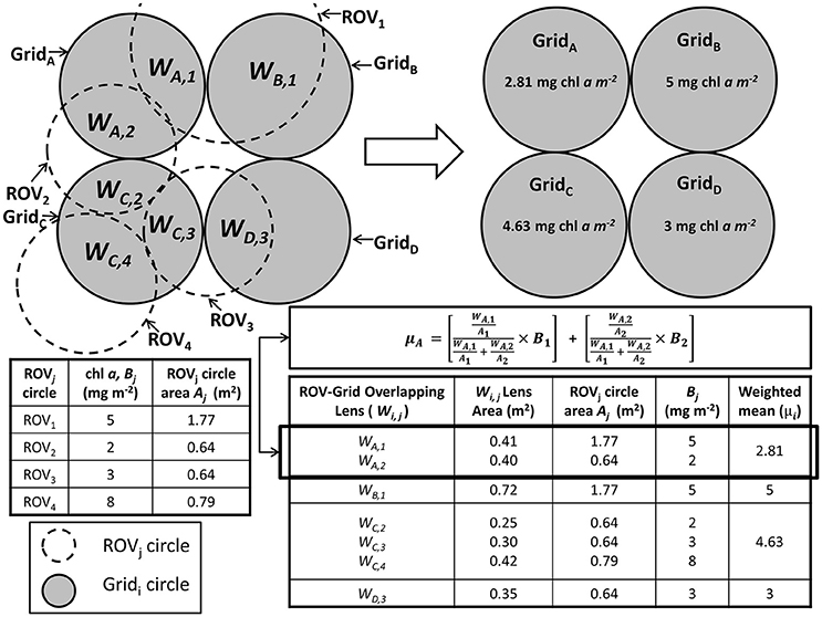
Figure 2. Detailed diagram and example calculation of the re-sampling process. A grid of circles was created for the ROV measurements (e.g., ROV1−4 circles) with each circle's center location determined by the measurement location (x, y) and the diameter determined by the footprint of the measurement. An additional grid of circles (e.g., GridA−D circles) was created where each adjacent circle was spaced 1 m apart and each had a diameter of 1 m. For each grid circle (e.g., GridB and D) with only one overlapping ROV circle (e.g., ROV1 and 3, respectively), which had an overlapping area ≥0.2 m2 (e.g., WB,1 and WD,3, respectively), the corresponding ROV-based transmittance and chl a were assigned to that grid circle. For each grid circle (e.g., GridA and C) that had more than one overlapping ROV circle (e.g., ROV2−4 and ROV1−2, respectively), of which at least one ROV circle had an overlapping area ≥0.2 m2 (e.g., WA,1-2 and WC,2-4, respectively), weighted means (e.g., μA for GridA chl a) of the corresponding ROV-based transmittance, draft and chl a were assigned to the grid circle. Weighting factors were calculated as the overlapping area of each ROV circle with the corresponding grid circle divided by the sum of all overlapping areas for that grid circle.
ROV-Derived Net Primary Production Estimates
All NPP estimates were calculated based on the re-sampled ROV observations of chl a and transmittance. Up-scaled daily ice algal NPP estimates, P (mg C m−2 d−1), were calculated using the photosynthesis equation from (Platt et al., 1980):
where is the chl a-normalized maximum fixation rate with no photoinhibition (mg C [mg chl a]−1 h−1); αB is the initial slope of the saturation curve (mg C [mg chl a]−1 h−1 [μmol photons m2 s−1]−1); and βB is strength of photoinhibition (same units as α). , αB, and βB correspond to the photosynthetic parameters determined by Fernández-Méndez et al. (2015) using the 14C method and incubating for 12 h, based on ice core samples collected from the same seven ice stations. Derivation of the photosynthetic parameters was conducted for upper-half and lower-half portions (mean: 0.58 m; range: 0.40–0.98 m) of the sea ice melted at 4°C in the dark for 24 h. NPP estimates were only calculated and compared for the bottom ice portions because previous in situ incubations studies demonstrated bottom-ice had the highest primary production rates, despite lower irradiance levels (Mock and Gradinger, 1999). Furthermore, because sea ice algal chl a biomass typically accumulates in the bottom-ice portion it is safe to assume a large majority of the primary production also occurred in the bottom-ice. Accordingly, we used only chl a biomass estimates for the lower portion, where 75% of the total chl a biomass was observed Fernández-Méndez et al. (2015). ROV-based chl a correspond to the total chl a biomass within the entire ice column, therefore we multiplied by 0.75 to get the appropriate fraction of the total chl a in the bottom ice portion. B represents the bottom-ice algae chl a concentrations derived from ROV-based spectral transmittance measurements. It is the hourly-averaged transmitted PAR (μmol photons m2 s−1) at the ice-water interface, converted to bottom-ice scalar irradiance according to Katlein et al. (2014), and calculated for each hour (t) over a 24 h period (t = 1, 2, … 24) by multiplying the ROV spectral (PAR) transmittance by hourly-averaged (t) incoming PAR (μmol photons m2 s−1) measured during each ice station.
Statistical Analyses
All statistical analyses were conducted using R software Version 2.15.2 with all relevant packages (R-Development-Core-Team, 2012) listed after the corresponding analysis description.
Ice core chl a data used for comparison were presented in Fernández-Méndez et al. (2015), hereafter referred to as “FM” cores (1 core per station), and were melted in filtered sea water. Since the FM-cores were used to characterize the NPP for each ice station (Fernández-Méndez et al., 2015) we assessed the representativeness of the single cores compared to the up-scaled ROV surveys of chl a biomass and NPP. NPP was not measured on the LM-cores, thus we only compared NPP estimates for FM-cores with the ROV estimates, which had both chl a biomass and under-ice light measurements. FM-cores were considered representative of the area if they were within the interquartile range (IQR; 25–75 percentiles) of the up-scaled ROV and SUIT estimates.
Cores from Lange et al. (2016), hereafter referred to as “LA” cores (4–12 cores per station) were directly melted. For comparisons of chl a biomass between ice core and ROV-derived estimates and between level ice and ridged ice, FM and LA cores were grouped together, referred to as CORES. The significance of differences between these groupings was assessed using the non-parametric Wilcoxon rank sum test (Wilcoxon, 1945). We used a non-parametric test because the assumption of normality required for parametric tests (e.g., t-test) could not be achieved for the entire datasets using common data transformation methods (e.g., log, square root, squared, cube-root).
The relative importance of each variable (B and It), in terms of explaining the variance of NPP for each ROV station, was assessed using the coefficient of determination (R2) for all up-scaled NPP estimates (Pt) vs. chl a (B) estimates (i.e., explained variance due to chl a), and NPP estimates (Pt) vs. bottom-ice light (It) observations (i.e., explained variance due to light). The R2 was calculated for each hour (t) of the 24 h period to capture the diurnal variability of light conditions. Values provided in Table 1 correspond to the daily mean R2.
Spatial Autocorrelation Analyses
Spatial autocorrelation was used to investigate the horizontal patchiness of sea ice draft, transmittance, chl a biomass and NPP measured at the seven ice stations (Table 1). Autocorrelation was estimated using Moran's I (Moran, 1950; Legendre and Fortin, 1989; Legendre and Legendre, 1998), which was calculated for each of the eight sites at equally spaced (3 m) distance classes. Individual autocorrelation coefficients or Moran's I estimates were plotted for each distance class in the form of a spatial correlogram (Legendre and Fortin, 1989; Legendre and Legendre, 1998). These analyses were conducted using the “R” software function correlog from the “pgirmess” package. Autocorrelation coefficients for each distance class were assigned a two-sided p-value following methods in Legendre and Fortin (1989) and Legendre and Legendre (1998). Global significance was determined on the correlogram using the Bonferroni-corrected significance level. The presence of spatial autocorrelation (i.e., spatial patterns or patchiness) was determined if the correlogram was globally significant at p < 0.05. We identified the first x-intercept of globally significant correlogram lines as the patch size (P) of the variables (Legendre and Fortin, 1989; Legendre and Legendre, 1998). Here, patches were identified for sea ice draft (Pd), transmittance (Pt), chl a biomass (Pc), and NPP (Pp). This methodology is consistent with spatial autocorrelation analyses used in other snow and sea ice studies to identify patch sizes of both biological and physical variables (e.g., Gosselin et al., 1986; Rysgaard et al., 2001; Granskog et al., 2005; Søgaard et al., 2010).
We classified the correlograms according to correlogram curve patterns described in Legendre and Legendre (1998): (i) multiple-bumps; (ii) wave-like structure; (iii) single bump; (iv) gradient; (v) step; or (vi) random. Because we do not have fully gridded data, it is difficult to differentiate between i) vs. ii), or iv) vs. (v), as the correlograms are very similar. Therefore, we combined these pattern types together resulting in four categories (1) multi-bump/wave; (2) one-bump; (3) gradient/step; and (4) random/noisy. Interpretations of the correlograms together with the xy gridded maps allowed for more detailed interpretation of the patterns (Legendre and Legendre, 1998). Patches or regions of high chl a biomass, high transmittance, thick draft, and high NPP were identified manually by visually inspecting the gridded maps. The identified patches were compared between variables to identify coincident patches for different variables.
Results
Sea Ice Algal Chl a Biomass Estimates
The median chl a concentrations were generally low (< 3.0 mg m−2) at sampling locations A-H, irrespective of the method used (Table 1). Only at location I, median chl a concentrations were above 4 mg m−2 for ice core and ROV estimates (Table 1). The range of chl a concentrations observed, however, appeared to be greater at locations G to I compared to locations A to F (Figure 3A).
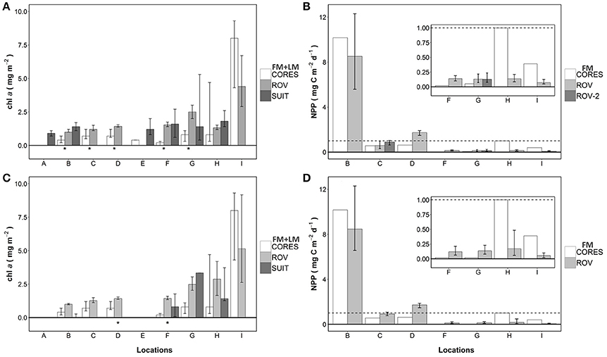
Figure 3. Chl a and NPP summarized per sampling gear and location, and subset into dominant ice classes. (A) chl a biomass for the entire datasets of each sampling gear; (B) NPP for the entire datasets of each sampling gear; (C) chl a estimates from only the dominant ice class; and (D) NPP estimates from only the dominant ice class. Dominant ice classes for each location are listed in Table 3. Bars represent median and error bars the interquartile range. *Indicates significant Wilcoxon rank sum test at p < 0.05 between the CORES and ROV data for the corresponding location. (A,C) CORES are the combined datasets of FM-CORES, data from Fernández-Méndez et al. (2015); LA-CORES, data from Lange et al. (2016). (B,D) CORES are only the FM-CORES.
At 5 of the 7 locations sampled for ice cores and ROV measurements, (B-D, F-G), sea ice cores had significantly lower chl a biomass than ROV estimates (Wilcoxon test, p < 0.05). No significant differences were observed at locations H and I (Wilcoxon test, p > 0.05; Table 1; Figure 3A). On average, ice core-based estimates of chl a concentration were 63% of the ROV-based estimates from the same sampling sites. The range was 13–62% for locations B to H, however, location I was substantially larger at 182%. Excluding location H results in a mean underestimation of core based estimates of 43% compared to ROV based estimates. There was no significant difference between integrated estimates of sea ice chl a concentrations of ROV and nearby SUIT profiles (Wilcoxon test, p < 0.05).
FM-cores were not representative (i.e., within the IQR) of the ROV-derived chl a biomass estimates at all locations, except location B (Table 1). FM-cores at location C, H, and I, over-estimated chl a biomass compared to the ROV-derived estimates (Table 1). At locations D, E, F, and G the FM-cores under-estimated chl a biomass compared to ROV-derived estimates (Table 1). When chl a estimates were combined by FYI and MYI stations for each sampling method, mean FM-core chl a estimates were considerably lower than spatially integrated ROV- and SUIT-based estimates, but these differences were not significant due to the large variability of the datasets (Wilcoxon test, p > 0.05; Table 2). Regardless of the sampling method, MYI stations had consistently higher chl a concentrations and lower PP rates than FYI stations (Table 2).
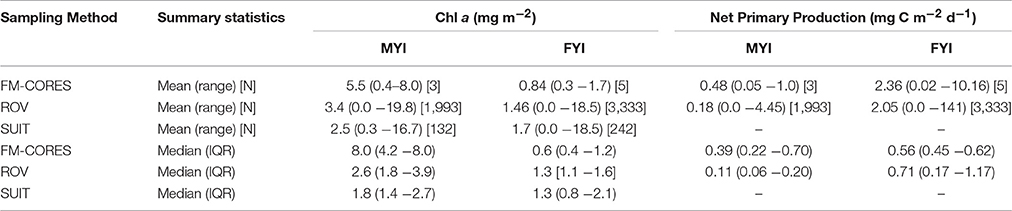
Table 2. Ice algal chlorophyll a biomass and NPP summarized for sampling gears into MYI and FYI. Means, range (min–max), and sample size [N] are provided for comparison to values presented in Fernández-Méndez et al. (2015).
All gridded ROV surveys of chl a, sea ice draft, transmittance and NPP are shown in Figures S1–S8. SUIT profiles of chl a, sea ice draft, and identified ridges are shown in Figures S9–S16.
ROV-Derived Sea Ice Algal NPP
We accounted for the spatial variability of NPP by combining the variability of both chl a and bottom-ice light in the calculations of the larger-scale NPP estimates. All gridded ROV surveys of NPP are shown in Figures S1–S8. We then determined the explained variance of NPP by each variable individually. At locations B, C, F, G, and I, the spatial variability of bottom-ice light explained most of the spatial variability of the up-scaled NPP estimates, whereas at locations D and H, chl a explained most of the spatial variability of NPP (Table 1; Figure 4).
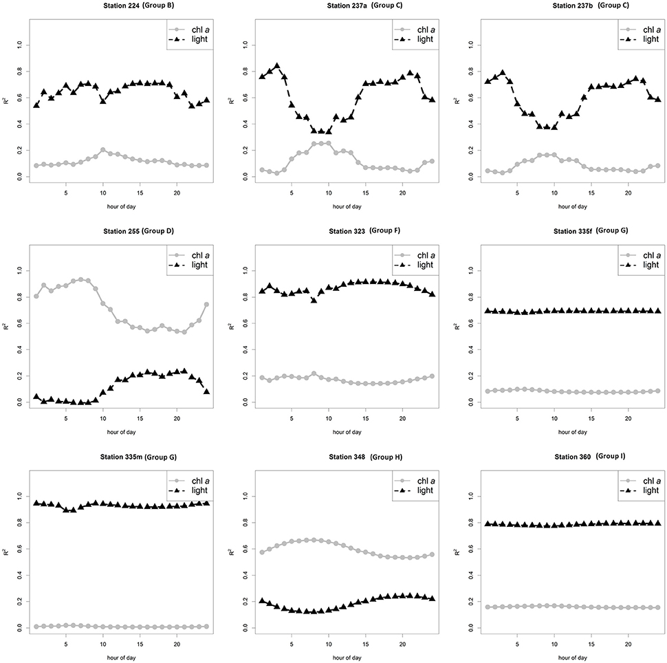
Figure 4. Explained variance (R2) of NPP by up-scaled chlorophyll a and bottom-ice PAR (light) per hour for each ROV station and survey listed in Table 1.
The largest diurnal variabilities of light levels and explained variances were observed at locations with the highest mean bottom-ice light levels (Table 1; Figure 4). At all stations, the explained variance of chl a was inversely related to light, which is expected since NPP is a function of both variables and chl a estimates were constant over the diurnal cycle while only light varied. The inter-location differences regarding which variable (chl a or light) explained most of the variance in NPP cannot be stated for certain as we observed no significant correlations between the explained variance for each station and any other station variable (e.g., nutrient concentration, median and IQR chl a or bottom-ice light).
FM-core NPP estimates were representative (i.e., within the IQR) of the up-scaled estimates at station group B and one ROV survey at station group C (Table 1; Figure 3B). FM-cores under-estimated NPP at station groups C, D, F, and G, and over-estimated NPP at station groups H and I compared to the up-scaled ROV-based NPP estimates (Table 1; Figure 3B). The differences between methods were likely the result of differences in chl a and/or light. Location B had similar chl a biomass and NPP for both the FM-core and up-scaled estimates (Table 1; Figures 3A,B). Station groups D, F, and G had higher up-scaled chl a biomass and NPP estimates compared to FM-core estimates (Table 1; Figures 3A,B). Conversely, station groups H and I had lower up-scaled chl a biomass and NPP estimates compared to FM-core estimates (Table 1; Figures 3A,B). Only station group C had higher chl a biomass but lower NPP estimates for the FM-cores compared to the up-scaled estimates (Table 1; Figures 3A,B). Furthermore, light levels were comparable (237a) or slightly higher (237b) for the FM-core derived NPP estimates compared to the ROV surveys (Table 1; Figures 3A,B). When FM-cores and the up-scaled NPP estimates were pooled into FYI and MYI stations, we observed no significant differences between the methods (Wilcoxon test, p > 0.05; Table 2). The median and IQR-values had large differences between sampling methods for the MYI stations but the mean values were similar (Table 2).
Sea Ice Algal Chl a Biomass and NPP in Relation to Sea Ice Properties
Sea Ice Classes
Chl a biomass and NPP estimates were divided into the five different ice classes. The values showed large variability between ice classes and locations, and within ice classes and locations (Figure 5). ROV-derived chl a biomass estimates at locations B and I were highest in the thickest sea ice class (2.0 m +; Figure 5A). Locations B and C had high ROV-derived chl a biomass in the thinnest ice class (0.0–0.5 m; Figure 5A). The three middle ice classes generally had uniform ROV-derived biomass estimates, with the exception of location H which had the highest ROV-derived chl a biomass in the 1.5–2.0 m ice class (Figure 5A). The SUIT-derived estimates were very low at location B for all ice classes and highly variable within the ice classes for all other stations with no obvious patterns (Figure 5C). In general, at each location ROV-derived NPP estimates showed a decreasing trend with increasing range of ice class thickness values (Figure 5B).
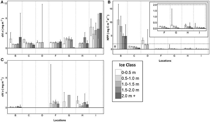
Figure 5. Summary of chlorophyll a and NPP estimates per ice class and location for: (A) ROV derived chlorophyll a biomass; (B) ROV-derived NPP estimates; and (C) SUIT derived chlorophyll a biomass estimates. Bars represent median and error bars the interquartile range. †Indicates missing values.
The dominant ice class surveyed by the ROV was identified by the modal sea ice draft of ice floes based on EM31 measurements (Table 3). Ice core and ROV chl a biomass estimates for the dominant ice classes differed significantly (Wilcoxon test, p < 0.05) at 2 locations (F,G; Table 3; Figure 3C). NPP estimates derived from FM-cores and ROV observations showed no obvious changes and maintained the same patterns (i.e., non-representativeness) for all locations. Most obvious differences were observed between the entire chl a biomass surveys and dominant ice class subsets for the SUIT at locations B, F and G, and for the ROV at locations H and I (Tables 1, 3; Figures 3A,C). Furthermore, the separation between low chl a biomass locations B to F and high chl a biomass locations G to I is more obvious from the large scale dominant ice class estimates (Figure 3C).
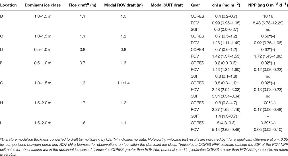
Table 3. Modal sea ice draft from literature (Boetius et al., 2013; Katlein et al., 2015b) and ROV measurements, dominant ice class based on literature modal draft, interquartile range of chlorophyll a biomass observations for the dominant ice class using different gears (ice coring, ROV, and SUIT) summarized for each location.
Two sea ice regimes were identified at station 349 of group H: one thicker sea ice region and one thinner region (Figure S7). The thicker region (median: 1.9, IQR: 1.2–3.5 mg chl a m−2) had significantly higher (Wilcoxon test, p < 0.05) chl a biomass than the thinner region (median: 1.3, IQR: 1.2–1.4 mg chl a m−2). NPP, however, was significantly lower at the thicker region (median: 0.07, IQR: 0.04–0.19 mg C m−2 d−1) compared to the thinner region (median: 0.14, IQR: 0.12–0.21 mg C m−2 d−1). Ice cores from the thicker region had higher chl a biomass (median: 0.3, IQR: 0.2–0.5 mg chl a m−2) compared to ice cores from the thinner region (median: 4.6, IQR: 2.8–6.2 mg chl a m−2) although the p-value of the Wilcoxon test was 0.06 due to the low sample size.
Sea Ice Ridges
At ice location B (station 224; Figure 1) we identified two sea ice ridges based on the ROV draft measurements (Figure 6A). Ridge 1 had a median sea ice draft of 4.5 m and ridge 2 had a median draft of 2.8 m based on ROV measurements (Table 4). Bottom-ice light was significantly higher in level ice compared to both ridges (p < 0.05; Table 4). Nonetheless, both ridges had significantly higher ice algal chl a biomass than the level ice (p < 0.05; Table 4; Figure 6C). Ridge 2, however, had significantly lower NPP compared to level ice, whereas ridge 1 had similar NPP compared to the level ice (Table 4; Figure 6D). Conversely, ridge 1 had both higher draft values and higher bottom-ice scalar irradiance values I at the bottom compared to ridge 2 (Table 4; Figures 6A,B,D). In the level ice, chl a biomass and bottom-ice light explained comparable amounts of the NPP variance. At ridges 1 and 2, however, chl a biomass explained relatively more variance compared to bottom-ice light (Table 4).
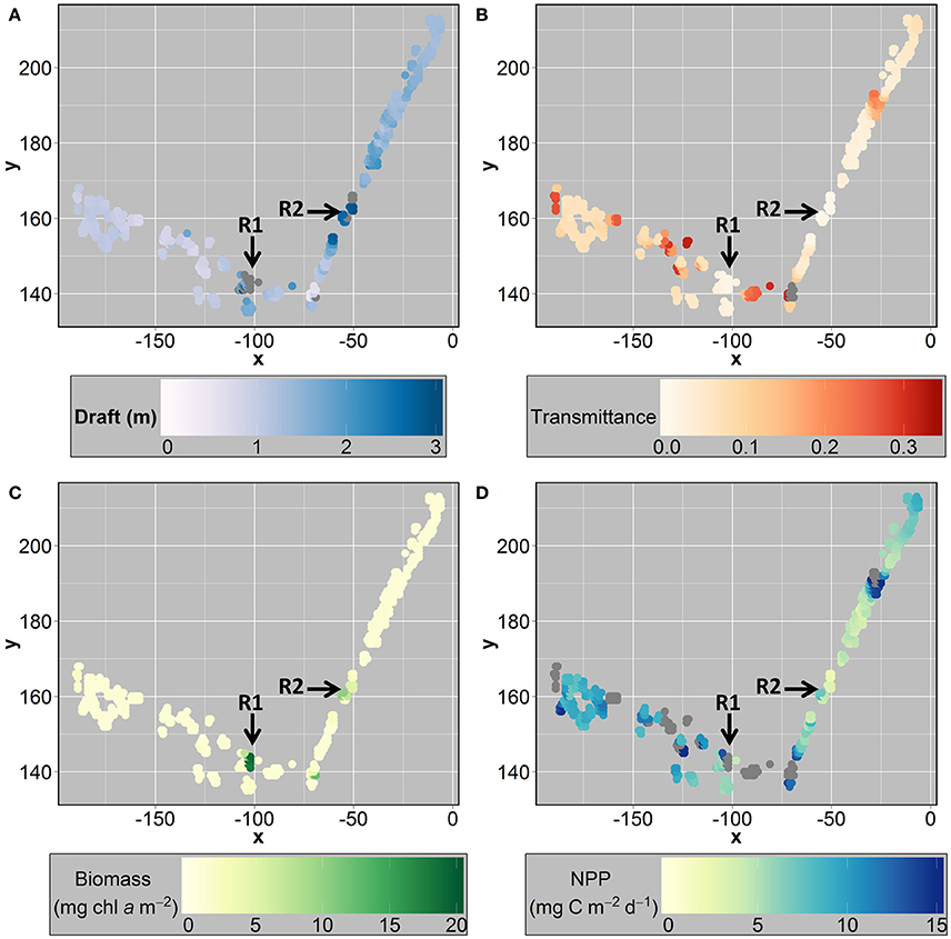
Figure 6. Gridded x-y (meters) map of the remotely operated vehicle (ROV) station 224, showing: (A) draft (m); (B) transmittance; (C) chlorophyll a biomass (mg m−2) derived from ROV spectral radiation measurements; and (D) net primary production-NPP (mg C m−2 s−1) derived from ROV measurements. R1 and R2 depict ridge 1 and ridge 2, respectively. Gray circles represent values greater than the scale maximum value.

Table 4. Comparison of chlorophyll a biomass and net primary production between sea ice ridges and level ice at station 224.
Based on the ridge identification analysis for all SUIT stations we calculated a mean (min–max) ridge density of 7.5 ridges km−1 (2.5–18.0), mean ridge width of 68.7 m (47.6–100.3), and a mean percent total ice coverage by ridges of 9.2% (2.5–15.4%). Ridge analysis summaries for each SUIT station are shown in Table 5. SUIT profiles with identified ridges are shown in Figure 7 (station 223) and for all other stations in Figures S9–S16.
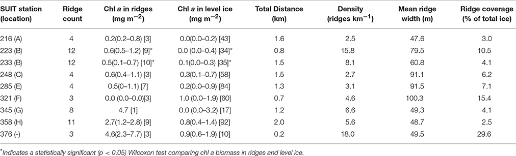
Table 5. Summary of ridge identification analysis from the SUIT hauls conducted during PS80.
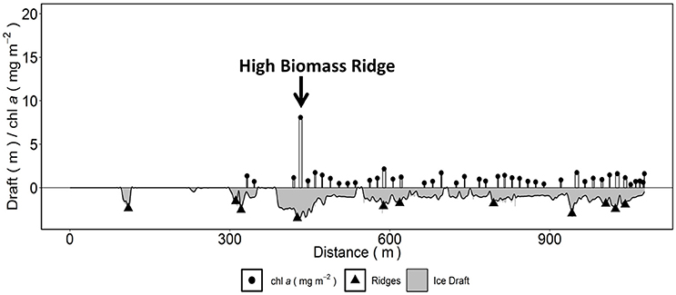
Figure 7. Horizontal profile of Surface and Under-Ice Trawl (SUIT) station 223 showing sea ice draft, identified ridges and chlorophyll a biomass derived from spectral radiation measurements. Highlighted is an identified high chlorophyll a biomass sea ice ridge. Width of the white bars corresponds to the relative along-track footprint of spectral radiation measurements. The black line corresponds to the smoothed sea ice draft curve used for the ridge identification procedure and was determined from the ice draft measurements (gray shaded area).
High chl a biomass sea ice ridges were also identified within three SUIT stations (station 223: Figure 7; stations 233, 285, and 358 Figures S11, S13, S16). These identified high chl a biomass ridges had chl a biomass estimates in the range 2–9 mg chl a m−2 (Table 5), which was larger than the overall SUIT profile median values in the range 1.2–1.9 mg chl a m−2 (Table 1). When comparing chl a biomass values at coincident identified sea ice ridges with chl a biomass at level ice for each SUIT haul separately, we observed significantly higher (Wilcoxon test, p < 0.05) sea ice ridge chl a biomass than level ice chl a biomass at 2 SUIT hauls (stations 223 and 233; Table 5). When comparing all SUIT observations combined, sea ice ridge chl a biomass (median: 0.7 and IQR: 0.2–1.4 mg chl a m−2) was significantly higher (Wilcoxon test, p < 0.05) than level ice chl a biomass (median: 0.3 and IQR: 0.0–1.0 mg chl a m−2).
Spatial Variability of Sea Ice Properties, Algae Chl a Biomass, and NPP
Autocorrelation analyses for each station were conducted using correlograms (i.e., Moran's I vs. distance classes), and were all globally significant at the Bonferonni corrected level (p < 0.05/n; n = the number of distance classes). Patch sizes, identified as the distance class at which the first zero value of Moran's I occurred in the correlograms, were highly variable between stations and between measured variables (Table 6). Patch sizes for chl a (Pc) had a lower range of values between 7 and 30 m, whereas patch sizes for transmittance (Pt), draft (Pd) and NPP (Pp) were slightly higher in the range 10–50 m (Table 6). Pt and Pp were comparable (within 5 m) at all ROV stations except 224, which had the two identified ridges. The shapes of correlogram curves were similar for transmittance and NPP for all station surveys (Figure 8 and Figures S17–S24). Correlogram shape comparisons for all stations were highly variable with no obvious patterns for all other measured variables (Figure 8 and Figures S17–S24).
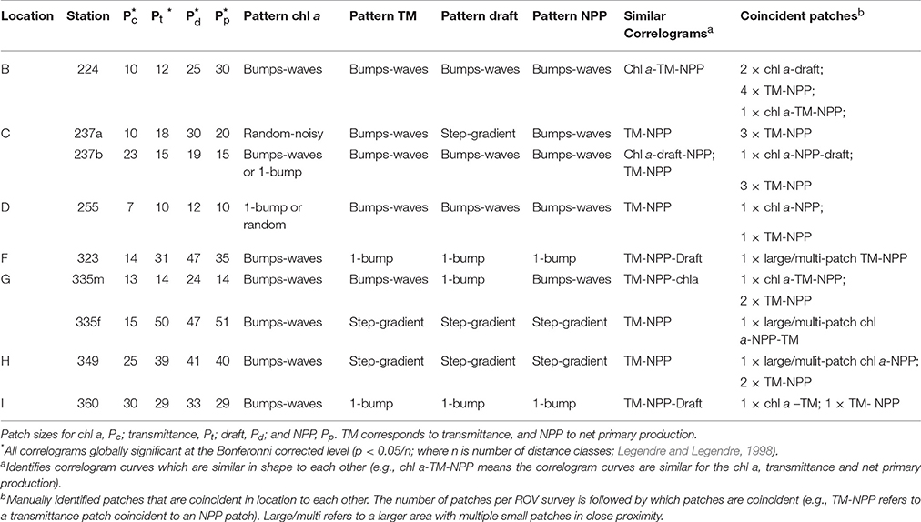
Table 6. Summary of the autocorrelation analyses per location and ROV survey.
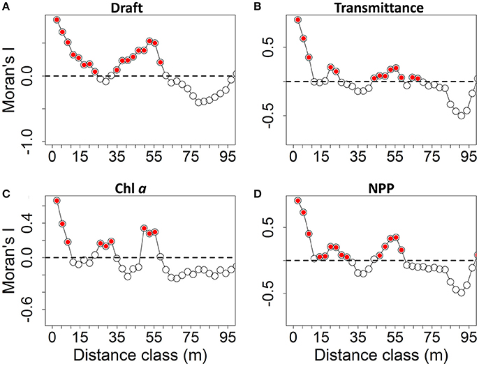
Figure 8. Correlograms showing Moran's I vs. distance classes at ROV station 224 for: (A) draft (m); (B) transmittance; (C) chlorophyll a biomass (mg m−2) derived from ROV spectral radiation measurements; and (D) net primary production-NPP (mg C m−2 s−1) derived from ROV measurements. Red filled circles represent significant values at p < 0.05.
Based on the manually identified patches within the gridded maps, coincident patches of high transmittance and high NPP were observed at all stations. Coincident patches of only high chl a and thick draft values were observed at stations 224 and 237b, although the patches at 237b were more subtle (Figure 6 and Figure S18). The two draft patches observed at 224 correspond to ridge 1 and ridge 2 (Figure 6) described in the previous section Sea Ice Ridges. Coincident patches of only high chl a, transmittance and NPP were observed at stations 224, 335f,m, and 360 (Figure 6, Figures S5, S6, S8). Coincident patches of only high chl a and NPP were observed at stations 255 and 349 (Figures S3, S7).
Discussion
Overall Representativeness of the Ice Algal Chl a Biomass and NPP Estimates Using Different Sampling Methods
Chl a Biomass
During land-based campaigns in coastal regions it is possible to achieve ice core sample sizes well over 50 ice cores (e.g., Gosselin et al., 1986; Rysgaard et al., 2001; Granskog et al., 2005; Mundy et al., 2007; Campbell et al., 2015). However, such studies are conducted over a period of weeks to months and are typically confined to a local study region. Furthermore, land-based studies are generally conducted on landfast sea ice, in regions dominated by seasonal sea ice. Thus, during the advanced melt stages in seasonally ice covered regions sampling sea ice is typically not done because it also coincides with the termination of the algal bloom, and/or due to logistical and safety constraints. Where sea ice survives into late-summer (e.g., the central Arctic Ocean), ship-based sampling is the most effective sampling approach. Although ship-based sampling has some advantages (e.g., bringing the equipment and lab to the study region), the main disadvantage is that sampling is generally time-limited. Thus, ice core sampling during ship-based campaigns is generally limited to < 10 algal chl a biomass or NPP cores per ice station making it difficult to conduct spatial studies of sea ice algae (e.g., this study; Gosselin et al., 1997; Gradinger, 1999; Schünemann and Werner, 2005; Fernández-Méndez et al., 2015). Even during long term ship-based studies (e.g., Melnikov et al., 2002) ice core sampling was limited to a small number of cores for each sampling interval every 1–2 weeks.
Our results demonstrate large uncertainties in coring-based methods for capturing the larger-scale variability of ice algal chl a biomass observed by the ROV-based methods. However, assessing the magnitude of this uncertainty for other studies is not possible. In general, our ice coring results under-estimated ice algal chl a biomass at the relatively lower chl a biomass locations (B-F), which implies an overall under-estimation of total chl a biomass. Only at the higher chl a biomass locations (H and I) the ice cores accurately captured the variability of ice algal chl a biomass. The higher chl a biomass observed at locations G-I was likely the result of less melt-induced algal losses due to thicker ice and lower melt rates at these high-latitude locations (Lange et al., 2016). This difference can be explained because at low chl a biomass stations relatively higher chl a biomass patches had a lower probability to be sampled by coring compared to higher chl a biomass stations, and hence were not accurately represented, whereas at high chl a biomass locations the probability of sampling higher chl a biomass locations was higher. We must also note that the possibility that the up-scaled spectrally derived estimates over-estimated the true chl a biomass is unlikely, because the model for spectrally deriving chl a biomass had no directional bias related to chl a concentration in sea ice (Lange et al., 2016).
The higher chl a biomass location I showed no significant difference between the cores and ROV-based chl a biomass estimates. In the individual core values, however (0.05, 6.46, 8.03, 8.00, and 11.83 mg chl a m−2), only one core was within the IQR (2.96–6.70 mg chl a m−2). In this sample size, one core with near-zero chl a biomass was highly influential and may have impeded the detection of significant differences. A similar pattern was also apparent at location H, which also showed no significant difference, but also had only one core within the IQR of the up-scaled chl a biomass estimates. The discrepancy between the ice core-based and ROV-derived chl a biomass estimates indicates the ice algal chl a biomass was highly variable at small scales (< 2 m), which was difficult to capture with average measurement footprints between 1 and 2 m for ROV surveys. Individual data points of up-scaled estimates averaged chl a concentration over a larger area, and were thus less likely to capture small patches of extremely high chl a biomass or extremely low chl a biomass (i.e., values in the range 8–12 mg chl a m−2 or with near-zero chl a biomass). These considerations highlight two important sampling constraints. First, the cores did not capture the large-scale variability; and second, we were unable to assess the small-scale variability below 2 m. The second limitation is less drastic since the signal received from the sensor under the ice does capture the small-scale variability within its measurement by averaging it over a larger distance. Since little is known or has been reported on summertime spatial variability of ice algal chl a biomass we propose that observations from both core-based and under-ice spectral profiling systems should be combined when making assumptions about multi-scale spatial variability of ice algal chl a biomass.
The fact that no statistical differences (Wilcoxon test, p > 0.5; Table 2) were observed between ROV-based and ice core-based estimates (both chl a and NPP) when they were grouped into MYI and FYI stations, an approach taken by Fernández-Méndez et al. (2015), may suggest an improvement because it increased the probability of the ice cores to be representative of the larger area. In this case the sample sizes and range of chl a biomass values were sufficient to obscure any differences at the station level. This method should only be considered when other options are not possible, because large uncertainties are still present even though significant differences were not found. For example, even though in this case the mean MYI FM-core chl a biomass values were not significantly different (Wilcoxon test, p > 0.05), each MYI FM-core value was higher or lower than the IQR of the larger-scale estimates. A similar pattern was observed with the FYI grouping comparison although not as drastic because overall the values were smaller, particularly the range of values. Potential uncertainties of grouping ice cores should also be considered depending on the objectives of your study. Grouping the ice cores into MYI and FYI would result in mean ice core MYI algal chl a biomass estimates 160% larger than the ROV MYI estimates. In contrast, FYI ice core estimates would be around 60% of the ROV FYI estimates. For grouped ice core-derived NPP the difference for MYI is even more pronounced at 270% larger compared to ROV estimates. FYI NPP values, however, were comparable between both methods.
Photoacclimation may be another potential factor influencing the chl a to carbon ratios, which could in turn explain the increased chl a biomass at higher latitude stations due to increased chl a production under lower light conditions. Fernández-Méndez et al. (2015) measured lower photoacclimation indices for the higher latitude stations (Ik; mean: 30 μmol photons m−2 s−1, range 17–45) compared to the lower latitude stations (mean: 60 μmol photons m−2 s−1, range: 34–77). However, we did not observe any variability (< 1 g C: g chl a) between high and low latitude stations in the chl a to POC ratios (data not presented here), therefore it is unlikely that photoacclimation explains the regional chl a biomass differences.
NPP
In general, NPP sampling involves measuring available PAR levels through a hole in the ice (Gosselin et al., 1997), which may produce higher than expected values due to the hole. PAR available for bottom-ice algae may also be modeled by using simple light extinction models (Fernández-Méndez et al., 2015). Both methods are established and regularly employed, however, both are limited in the fact that they do not account for the spatial variability of the bottom-ice PAR levels. During spring, ice algae are typically light-limited and therefore have higher chl a biomass where light levels are higher (e.g., Gosselin et al., 1986), assuming there is no or limited photo-inhibition. During our summer sampling period, however, we found no strong correlation at any station between the ROV-derived chl a estimates and available under-ice light (maximum spearman correlation coefficient, r = 0.22). This means the under-ice light and chl a varied independently of each other. This behavior is expected, because in late-summer biomass losses due to high melt rates have a dominant influence on bottom-ice biomass (e.g., Grossi et al., 1987; Lavoie et al., 2005; Lange et al., 2016). These conditions would not have sustained a bottom-ice algal community, and therefore even if light conditions were suitable for high primary production rates the NPP would have been almost zero if no algae were present. With an additional variable (i.e., melt), which can influence NPP, the spatial distribution of NPP may be more complex in late-summer than during the spring to summer transition making it even more important to understand and account for the spatial variability of both chl a biomass and the bottom-ice light field.
Location B had similar NPP estimates for the FM-core and up-scaled observations (Table 1; Figure 2), which we attributed to the similar chl a biomass estimates (Table 1; Figure 1). Even though light levels and chl a biomass were only slightly larger at location B compared to groups C and D, group B had NPP estimates almost an order of magnitude larger than groups C and D. This was attributed to the substantially higher value of the photosynthetic parameter determined for this station (Fernández-Méndez et al., 2015), compared to all other stations. This demonstrates that the combination of data from several stations, an approach described by Fernández-Méndez et al. (2015) and used by others (Mundy et al., 2011; Campbell et al., 2016), was not only able to improve the spatial representativeness of light and chl a but also accounted for the potential variability of the derived photosynthetic parameters. Our results suggest pooling ice core samples increases the chance for the samples to be representative of both chl a biomass and NPP estimates. Because of the large range of chl a biomass and NPP estimates, and the small number of samples, however, this approach can still carry a high risk of obtaining non-representative estimates (e.g., overestimates of up to 270% for MYI).
The same directional difference of chl a biomass and NPP observed between up-scaled and FM-core estimates for all station groups, except group C, suggests the differences between the FM-cores and up-scaled NPP estimates were driven by the differences in chl a biomass. This was further confirmed by the fact that the bottom-ice light levels used for each method were comparable for each station (Table 1). The opposing pattern of chl a biomass and NPP between up-scaled and FM-core estimates at location C, even though light levels were comparable, suggests that the spatial variability of both the chl a biomass and bottom-ice light had a combined influence on the observed differences that is not apparent from the overall survey estimates. The explained variance of NPP by chl a and light showed large diurnal variability and large inter-location variability, which indicates a complex and highly variable relationship between ice algal chl a biomass and light levels during our sampling period. These results emphasize the importance of accounting for both the spatial variability of ice algal chl a biomass and the bottom-ice light field in order to make representative NPP estimates. We must also note the possible influence of nutrients since we found a significant (p < 0.05) positive correlation (r = 0.46) between explained variance of NPP by chl a with sea ice NO3 concentrations (data from Fernández-Méndez et al., 2015), and a significant (p < 0.05) negative correlation between explained variance of NPP by bottom-ice light with sea ice NO3 concentrations (r = −0.55). These correlations provide some indication that the sea ice nutrient regime could have also had some influence on the relative (inter-station) importance of chl a biomass vs. light on NPP.
Gosselin et al. (1997) measured ice algal NPP of up to 300 mg C m−2 d−1 in the high Arctic Ocean (>87°N) during August. Our results for September in the high Arctic Ocean (station 360) were over 3 orders of magnitude lower than those found by Gosselin et al. (1997) in August for the same area. The large difference in NPP estimates between the studies could partially be explained by the higher incoming solar irradiance in August compared to September. However, upscaling results from Fernández-Méndez et al. (2015) for August were also substantially lower with a mean (range) of 5.8 (0.06–42) mg C m−2 d−1 and with a similar range of daily mean incoming solar irradiance (101–249 μmols photons m−2 s−1). Therefore, we applied the range of incoming irradiance values (~125–214 μmols photons m−2 s−1) observed at the high latitude stations (>87°N) during the Gosselin et al. (1997) study to this studies ROV survey at station 360. We used our observed chl a biomass and transmittance in order to calculate potential NPP under higher incoming irradiance conditions typical for August at these high latitudes. Overall NPP increased by nearly the same relative amount as the available light, however, with median values between 0.82 and 1.32 mg C m−2 d−2 (Table 7) this remains two orders of magnitude lower than ice algal NPP observed by Gosselin et al. (1997). This suggests that something other than available light is influencing these observed differences. This is likely explained by the fact that the Gosselin et al. (1997) estimates were dominated by the sub-ice algal species Melosira arctica, whereas Fernández-Méndez et al. (2015) measured primary production on ice samples with a lower contribution of M. arctica. Thus, our samples represent a good estimate for in-ice algal NPP, however, a conservative estimate for overall ice-associated NPP (Fernández-Méndez et al., 2015).

Table 7. Net primary production estimates for the ROV survey at station 360 with observed downwelling surface irradiance (PAR) and using different downwelling surface irradiance conditions as observed for the same region (>87° N) earlier in the season (~ mid-August) by Gosselin et al. (1997).
The explained variance of NPP by bottom-ice light compared to chl a using the increased incoming irradiance levels, which were observed in August at high latitudes by Gosselin et al. (1997), showed interesting differences (Table 7). As the incoming irradiance increased, the explained variance of chl a biomass also increased, while the explained variance of the bottom-ice light decreased to nearly equal values of 0.39 and 0.48, respectively, at an incoming irradiance of 214 μmols photons m−2 s−1 (Table 7). This indicates that under increased irradiance levels the spatial variability of chl a biomass becomes more important in terms of contribution to overall NPP estimates. Furthermore, these results suggest a complex spatio-temporal relationship of the relative importance of chl a biomass and available bottom-ice irradiance for NPP estimates, which can only be accounted for by characterizing biomass and under-ice light at spatial scales from meters to 100s of kilometers, and temporal scales accounting for diurnal and seasonal variations.
Sea Ice Algal Chl a Biomass and NPP in Relation to Sea Ice Properties
Sea Ice Classes
Electromagnetic (EM) sea ice thickness surveys are commonly used to representatively characterize the overall ice thickness distribution (Eicken, 2001; Haas and Eicken, 2001; Haas, 2004) and thus represent a reliable characterization of the dominant ice class for the surveyed floe and overall region. The differences between the ROV-derived and EM-derived modal draft values at several ice stations warranted the use of the EM data to determine dominant ice types. The range of modal ice thicknesses for locations B-G dominated by FYI (0.8–1.3 m) were consistent with previous studies that conducted large-scale airborne and floe-scale ground-based electromagnetic ice thickness surveys for the same region and season (Haas et al., 1997; Haas and Eicken, 2001; Rabenstein et al., 2010). The two locations H and I dominated by MYI had modal thicknesses between 1.6 and 1.8 m, which were also consistent with modal ice thickness values for second-year sea ice from the same region and season (Haas and Eicken, 2001).
Since the dominant ice type thickness value (i.e., modal ice thickness) is a commonly used metric to characterize the sea ice environment it stands to reason that sea ice algal chl a biomass from the dominant ice class would also provide a representative metric to describe the overall sea ice algal chl a biomass. Comparing the ice algal chl a biomass estimates solely from the dominant ice classes showed better agreement between ROV and ice core-derived values (Figure 3C). Therefore, we suggest that using chl a biomass estimates from the dominant ice class only may be an improvement on providing a single value, which is representative of the large scale sea ice algal chl a biomass for that region. There remain some limitations to this approach, since these estimates do not account for the chl a biomass of the other ice types/classes. Sampling other ice types/classes may be of particular importance in regions of low chl a biomass (e.g., station 224) where high chl a biomass features such as ridges may have a substantial contribution to the overall large-scale ice algae chl a biomass. A further step to improve these overall chl a biomass values could be to use the larger-scale ice thickness density distributions (data not available for this study) to provide weighting factors for chl a biomass values of each ice type/class.
The observed trend of higher chl a biomass at higher latitude stations was more obvious within the dominant ice class estimates (Figure 3C). This was previously attributed to enhanced melt-induced algal losses at lower latitude stations, although based on a smaller number of stations (Lange et al., 2016). Here we have a larger sample size covering a larger geographic region and confirmed the pattern related to latitude and the presence of thicker ice. Enhanced melt is a common mechanism for substantial losses of bottom-ice algae in summer (Grossi et al., 1987; Lavoie et al., 2005). Gosselin et al. (1997) also observed a shift from low to high bottom-ice chl a biomass with a shift from low to high latitude, which is consistent with our observed trend. Furthermore, the higher dominant ice class chl a biomass estimates between 2.5 and 5.1 mg chl a m−2 observed at the three high latitude, thicker ice (1.4–1.9 m) locations G–I is consistent with previous studies from high latitude regions of the central Arctic Ocean with bottom-ice algae concentrations in the range of 3–14 mg chl a m−2 (Gosselin et al., 1997), and up to 22 mg chl a m−2 (Melnikov, 1997).
Castellani et al. (2017) introduced a pan-Arctic Sea Ice Model for Bottom-Algae (SIMBA) coupled with a 3D sea-ice-ocean model and also showed that within the eastern Eurasian basin during late-summer (this studies sampling region/period) there was an increasing trend in bottom-ice algal chl a biomass from lower to higher latitudes. The SIMBA model, however, showed the opposite trend with increasing chl a biomass from higher to lower latitudes in the region from the North Pole toward the northern coast of Canada and Greenland (the Lincoln Sea) where the thickest ice in the Arctic Ocean is located. During late-summer Castellani et al. (2017) identified sea ice thickness as a main factor controlling bottom-ice chl a biomass by limiting basal melt-induced algal losses during a period of advanced melt. Based on observations alone, a purely latitudinal effect may have been identified as driving the large-scale spatial patterns of sea ice algae. Therefore, the modeling results of Castellani et al. (2017) emphasize the need for more observations in the region between Canada, Greenland and the North Pole (a region coined: the “Last Ice Area”), and that modeling studies are essential in the context of interpreting large-scale patterns of sea ice algae observations. Furthermore, the SIMBA model included different ice classes, such as sea ice ridges. The SIMBA results showed that ridges, though exhibiting lower peak chl a biomass compared to level ice, the maximum chl a biomass was reached later in the season compared to level ice. More information is required in order to accurately parameterize sea ice features such as ridges in pan-Arctic models, however, SIMBA is a big step forward in terms of including ice classes within models, which we have identified as an important component of sea ice algal spatial variability.
In contrast to chl a biomass, NPP estimates showed no improvement when comparing only the dominant ice class (Figure 3D). This suggests that NPP estimates require a different approach for up-scaling and parameterizing models. The complex and highly variable relationship between ice algal chl a biomass and light levels during our sampling period suggests that more representative sea ice algal NPP estimates may be achieved by accounting for the relative contribution of NPP within each ice type. This would involve using larger scale ice thickness estimates to assign weighting factors to each ice classes' NPP estimate. In the absence of larger scale observations it is not possible to discover the spatial patterns of sea ice algal chl a biomass and NPP, or assess if the ice cores are actually representative of the area. To further improve upon the large scale pan-Arctic NPP and chl a biomass estimates we suggest to integrate our five ice classes, together with weighting factors for each ice class (based on large-scale ice thickness surveys), into pan-Arctic studies (e.g., Fernández-Méndez et al., 2015). Accurately assessing sea ice associated NPP in models is of particular importance since it can represent a dominant portion of total (water plus sea ice) NPP in regions covered by sea ice for most of the year (e.g., Gosselin et al., 1997; Fernández-Méndez et al., 2015). In general, pan-Arctic models of NPP, which include sea ice contributions to NPP are very limited (e.g., Lee et al., 2015) highlighting the need for improved sea ice algae model parameterizations.
Sea Ice Ridges
One source of variability in sea ice chl a concentrations, light transmittance and derived NPP may be topographical features of sea ice, such as ridges. Sea ice ridges are often under-sampled due to the logistical challenges to sampling this type of ice. Despite this fact, sea ice ridges have been reported to host high abundances of sea ice fauna during advanced melt (Gradinger et al., 2010). Furthermore, in the northern Baltic Sea high chl a biomass were observed within the ice along the upper sides of sea ice ridges and within the interstitial spaces, typically present within the unconsolidated aggregation of ice blocks that form ridge keels (Kuparinen et al., 2007). Therefore, we specifically investigated sea ice ridges with the hypothesis that they could host high abundances of ice algae during advanced melt due to lower melt rates in these locations.
We showed that the identified sea ice ridges at ROV station 224 and all SUIT stations (measurements grouped together) had significantly higher chl a biomass than measurements under relatively more level ice (e.g., areas that are not ridges). It can be assumed that ridges were under-represented in the ROV sampling due to a preference for relatively uniform sampling sites. In SUIT profiles, the natural distribution of ridges was likely well-represented, because the sampled profile cannot be chosen after the deployment of the net. The overall difference between median level ice chl a biomass and median ridge chl a biomass from the SUIT surveys, however, was relatively small (0.4 mg chl a m−2). The small difference is likely the result of not all ridges having high chl a biomass.
Our results of sea ice ridge densities between 2.5 and 18.0 ridges km−1 are within the range of larger scale airborne surveys with mean ridge sail densities between 4.3 and 7.2 ridges km−1 (Rabenstein et al., 2010). With the high resolution (0.5 m) under-ice topography measurements, we were able to accurately estimate the widths of the ridge and determined that these features represented up to 10% of the total sea ice area. Together with the higher chl a biomass observed at sea ice ridges, this indicates that these features require more in-depth investigations and may have a significant impact on overall chl a biomass estimates and availability of food for under-ice organisms.
Gradinger et al. (2010) showed sea ice ridges had elevated concentrations of ice meiofauna and under-ice amphipods, which was attributed to the flushing of the sea ice and low-salinity stress imposed at the thinner sea ice environment. Sea ice ridges may also extend into higher salinity water below the highly stratified, fresher surface melt water, which accumulates adjacent to the ridges under thinner ice (Gradinger et al., 2010). These results suggest that higher ice algal chl a biomass at ridges may be the result of reduced flushing and lower environmental stress. Furthermore, the presence of high algal chl a biomass as a food source may provide an additional explanation for the observed accumulation of organisms at ridges by Gradinger et al. (2010).
In addition to the possibility of reduced flushing and lower environmental stress at ridges, we suggest that the thicker ice experienced lower melt rates than the surrounding level ice resulting in lower algal losses. Perovich et al. (2003) indicated that sea ice ridges experienced an overall greater amount of melt than the surrounding undeformed sea ice, which may appear to contradict our premise. The higher overall melt observed at ridges by Perovich et al. (2003), however, was partially attributed to a few very thick ridges extending deep into the water, which were experiencing melt the entire year even during winter. Except for one weekly measurement in August, the melt rates for ridges were lower than the mean and were among the lowest of all ice types for that entire month during advanced melt (Perovich et al., 2003).
NPP estimates for sea ice ridges showed some interesting patterns at ROV station 224. Although both ridges had significantly higher chl a biomass than the level ice, ridge 2 had significantly lower NPP rates than ridge 1 and the level ice, whereas ridge 1 and level ice were not significantly different. These differences were due to the available light measured under the different types of sea ice. The higher chl a biomass at ridge 1 compensated for lower light levels compared to the level ice, resulting in similar NPP estimates compared to the level ice. However, the chl a biomass at ridge 2 was not sufficient to compensate for the lower bottom-ice light levels. Even though ridge 2 had a thinner median draft (2.8 m) value compared to ridge 1 it still had lower light levels. This shows that ridges can have a considerable impact on the complex relationship between chl a biomass and available PAR for NPP estimates at larger spatial scales. Furthermore, these results imply that sea ice features such as ridges have a different and perhaps more complex relationship between available light and chl a biomass than the surrounding sea ice. As a consequence, ridges must be sampled representatively, and both the variability of bottom-ice light levels and the variability of chl a biomass are required to make representative large-scale ice algal chl a biomass and NPP estimates.
The identification of sea ice ridges as potential chl a biomass and NPP hotspots warrants further dedicated research of these features. Further work should include dedicated modeling of the (bio)optical properties of sea ice ridges, which would require ice core chl a biomass estimates from ridges and high spatial resolution spectral radiation measurements under ridges.
Spatial Variability and Patchiness of Sea Ice Properties, Algae Chl a Biomass, and NPP
Our results indicated high variability of patch sizes between locations, which suggests that there is large regional and temporal variability of ice algal chl a biomass. Patch sizes of algal chl a biomass were within the range of springtime chl a biomass patch sizes between 5 and 90 m (Gosselin et al., 1986; Rysgaard et al., 2001; Granskog et al., 2005; Søgaard et al., 2010). However, the upper limit of this range is nearly the scale of some ROV surveys. The above mentioned studies were limited to the spring and found that ice algal chl a biomass and NPP typically followed the light regime (Gosselin et al., 1986; Rysgaard et al., 2001; Granskog et al., 2005), which is primarily controlled by the overlying snow pack (Perovich, 1996). Furthermore, these studies were conducted on uniform, landfast sea ice from coastal regions and thus are not representative of sea ice from the central Arctic Ocean. During our study, we also found that patch sizes and spatial variability of NPP was controlled primarily by light availability, albeit in the absence of snow. This was evident by the high explained variance of NPP by bottom-ice light, the similarity of NPP and transmittance correlogram curves, and the coincidence of high NPP patches with high light transmittance. Similar to a recent study by Campbell et al. (2017) that demonstrated a disjoint in ice algal carbon biomass and NPP over the spring to summer transition period, our chl a biomass patches did not always follow the light and NPP regimes, which clearly illustrates one key difference between the spring and summer ice algal communities.
We also demonstrated that patches of high NPP were associated with patches of high chl a biomass in the absence of high light availability. The fact that both chl a and transmittance show spatial patterns consistent with NPP patterns is not surprising given the fact that NPP estimates were calculated from light and chl a biomass. However, this emphasizes the need to account for the spatial variability of both the bottom-ice light and chl a biomass to properly characterize the spatial variability of NPP in order to make accurate large-scale estimates. At a few stations (most notably 360), however, we did observe high chl a biomass patches directly adjacent to high transmittance locations (e.g., melt ponds). NPP was also high at the high transmittance locations and the adjacent high chl a biomass patches creating one high NPP patch. We propose that the presence of high chl a biomass adjacent to high transmittance regions could be explained by a combination of lower melt rates in the thicker ice adjacent to high transmittance regions and increased bottom-ice light levels due to horizontal light scattering from e.g., melt ponds. This would have allowed for higher NPP rates and increased accumulation of chl a biomass while having reduced melt-induced losses, however, we note that more work is needed to confirm this hypothesis.
Sea Ice Algae Sampling Recommendations
In this section we provide some recommendations for conducting the most representative sea ice algae sampling possible under the typical time limitation of an ice station on this cruise of ~8 h. We assume that the dominant ice class (e.g., modal ice thickness) is known before sampling. Knowledge of the dominant ice class is important to ensure representative sampling; however, this depends on the objectives of the study. Knowledge of the spatial distribution for all ice types and classes will provide the best sampling protocol since a representative sample of each ice type/class will provide the most accurate and reliable estimates for the region.
Ice Core Chl a Biomass and NPP
A nested approach has been outlined in Miller et al. (2015), which identifies four hierarchical levels of sea ice sampling. We suggest, however, some modifications for sampling during summer. If the main objective of the study is to acquire one representative ice algal chl a biomass value for that ice station, then we suggest following the quaternary scale of the nested approach according to Miller et al. (2015) by extracting replicate cores (N = 3) within a small area (< 2 m). This accounts for the small scale variability. The tertiary scale of the nested approach should be selected based on ice type/class. Here we have demonstrated that a representative chl a biomass value may be best estimated by the dominant ice class (NOTE: this should only be considered if additional sampling is not possible). Therefore, ice cores should be sampled in triplicate (quaternary scale) at three different dominant ice class locations (tertiary scale).
To capture the spatial variability of chl a biomass using ice coring alone, all ice classes should be considered. The nested approach should sample triplicate ice cores (quaternary scale) at 10 m intervals (tertiary scale) based on our observed patch sizes between 10 and 30 m. We further suggest that the replicates and direction of tertiary scale transects should be designed to capture all ice classes. A systematic approach would be to classify the sea ice using 0.5 m interval classes (as presented here). The sample design must also consider other ice types such as melt ponds, bare ice and thick ice features (e.g., ridges and hummocks). We must also note that the time requirements for conducting a spatial variability study using ice coring will be highly variable depending on season and ice conditions. For example, to quantify the spatial variability of thick MYI in early spring over a distance of 100 m (e.g., 3 cores at 11 sites = 30 cores) would take 30 h (based on previous experience coring spring MYI). This same task could be accomplished by an ROV with a typical deployment time of 8 h for two perpendicular survey transects of 100 m.
We demonstrated that NPP estimates have a complex relationship between light and chl a biomass. Therefore, in order to acquire a representative estimate the spatial variability of both the under ice light field and chl a biomass must be accounted for. We suggest a nested approach similar to that proposed for assessing the spatial variability of ice algal chl a biomass. Triplicate ice cores (quaternary scale) should be sampled at 10 m intervals (tertiary scale). In general, nested NPP sampling schemes should be conducted at the 5 different ice classes, as proposed earlier (N = 15).
ROV Chl a Biomass and NPP
ROV surveys should be conducted either over a grid or perpendicular transects with at least 60 m axis lengths in both directions for chl a biomass (two times maximum patch size of chl a) and at least 100 m for NPP estimates (two times maximum patch sizes for TM and NPP ~50 m). This ensures you cross the boundary of the patch at least once. The survey should be chosen so that it covers these dimensions depending on the objectives of the study. However, the main criteria for setting transect/grid dimensions should be so that all 5 ice classes are surveyed (or all identified ice classes for the study site), of particular importance is the inclusion of unique and under-sampled sea ice features such as ridges or MYI hummocks (Lange et al., 2017). As we have shown, even over distances of 100 m the dominant ice classes and all ice features such as ridges were not representatively sampled. This is partly due to the location chosen and also due to filtering of the data resulting in inconsistent sample spacing-coverage. This in turn may over-sample some regions compared to others and result in non-representative surveys for certain ice classes. Therefore, we recommend that care is taken to choose ROV transects or grids that cover all ice classes, and to ensure ROV measurements are conducted while minimizing distance to the ice bottom, and pitch and roll angles.
During data analyses one should always consider the dominant ice class for the corresponding region based on larger scale ice thickness surveys. Because universal algorithms are not yet available for deriving chl a biomass from spectral radiation, ice cores should always be conducted at as many locations as possible along the ROV surveys for training bio-optical models, deriving photosynthetic parameters for up-scaling ROV NPP estimates and subsequently to parameterize algae models. Because the time requirements for ice coring (this does not include laboratory processing times) at the distances required for spatial variability studies (e.g., >100 m) are likely much greater than a typical ROV deployment of 8 h, we strongly recommend to conduct both ROV and ice core sampling particularly for spatial variability studies of both chl a biomass and NPP.
This method does have limitations in terms of assessing the temporality of ice algal chl a biomass and NPP due to the limited period of sampling and logistical constraints. This is a common drawback in observational sea ice biogeochemistry, which results from the limitations of sample processing and incubation times, and the shear difficulty of sampling within the Arctic Ocean in order to cover the necessary periods of weeks to months. However, our approach showed the successful application on spatially extensive datasets and thus is an ideal approach that should be applied to long-term studies (e.g., ice-tethered sensor arrays; Nicolaus et al., 2010) in order to assess the short- to long-term temporal variability of ice algal chl a biomass and NPP.
Conclusions
We provided, for the first time, a detailed multi-scale comparison of ice-core based ice algal chl a biomass and NPP estimates with estimates derived from under-ice spectral radiation measurements conducted over distances of tens to thousands of meters. These approaches demonstrated substantial improvements regarding representative sea ice algae observations. Our results showed that ice core-based estimates of summertime ice algal chl a biomass and NPP do not representatively capture the spatial variability compared to the spatially more extensive estimates of moving platforms. This may carry similar uncertainties, with an overall negative bias of ~60%, for pan-Arctic estimates based on ice core observations alone.
Our autocorrelation analyses showed patch sizes of algal chl a biomass (10–30 m) and NPP (10–50 m) that were highly variable between locations and with scales of variability unlikely to be captured by ice coring alone. Based on our results we presented sampling recommendations depending on the objectives of the study. To estimate ice algal chl a biomass alone, taking a representative sample (N = 3) of each ice type/class using the ice core method should provide a reliable estimate of the overall area if there is also knowledge/observations of the ice thickness distribution on large scales (>1 km). Upscaling chl a biomass estimates would benefit from sampling all ice classes and factoring in weights for the spatial coverage of different ice classes in the region of interest. For NPP estimates, however, a combination of larger scale (>100 m) under ice light and ice algal chl a biomass is required because of the independent relationship between light and chl a biomass during the end of summer. In order to get the most representative estimates and to address the spatial variability of chl a biomass and NPP, we recommend that future sea ice sampling should combine ice-core based methods with the larger-scale under-ice spectral profiling approaches presented and described here and in Lange et al. (2016). This combined approach is also logistically justified since the time requirements for ice coring, which does not include processing times, at the distances required for spatial variability studies are typically much greater than a typical ROV deployment of 8 h.
We also identified high chl a biomass ridges within several up-scaled surveys, which have been generally neglected in sea ice biogeochemical studies. Sea ice ridges had significantly higher chl a biomass than the level ice and accounted for up to 10% of the total areal ice coverage. This suggests that these features may represent important regions for sea ice algal growth that are not easily captured by ice coring methods due to logistical difficulties of coring such thick sea ice. Further dedicated sea ice ridge studies are warranted particularly in terms of ice algal chl a biomass, nutrients, primary production and bio-optical properties.
Author Contributions
This study was designed by BL, CK, MN, IP, and HF. Data acquisition were performed by BL, CK, MF-M, MN, IP, and HF. Data analyses were performed by BL, GC, CK, MF-M, MN, IP, and HF. Interpretation of the results were performed by BL, CK, GC, and HF. Drafting the first version of the manuscript was done by BL with critical revisions and important intellectual additions by all other authors (CK, MN, GC, IP, MF-M, and HF) during all stages of manuscript preparation. All authors give final approval for the publication of this manuscript in its current form.
Conflict of Interest Statement
The authors declare that the research was conducted in the absence of any commercial or financial relationships that could be construed as a potential conflict of interest.
The reviewer TJ and handling Editor declared their shared affiliation.
Acknowledgments
We thank Captain Uwe Pahl, the crew, and scientific cruise leader Antje Boetius of RV Polarstern expedition PS80.3 (ARK27-3; IceArc), for their excellent support and guidance with work at sea. We thank Martin Schiller for his technical expertise and operational support during ROV deployments. We thank Jan Andries van Franeker (IMARES) for kindly providing the SUIT and Michiel van Dorssen for technical support. SUIT was developed by IMARES with support from the Netherlands Ministry of EZ (project WOT-04-009-036) and the Netherlands Polar Program (project ALW 866.13.009). We acknowledge the collaboration and technical support by Ocean Modules, Sweden for development and deployment of the ROV. This study is part of the Helmholtz Association Young Investigators Group Iceflux: Ice-ecosystem carbon flux in polar oceans (VH-NG-800). We also acknowledge the Alfred-Wegener-Institut, Helmholtz-Zentrum für Polar- und Meeresforschung for essential financial and logistical support. All data are available from the PANGAEA databases: doi: 10.1594/PANGAEA.833292; and doi: 10.1594/PANGAEA.834221.
Supplementary Material
The Supplementary Material for this article can be found online at: https://www.frontiersin.org/articles/10.3389/fmars.2017.00349/full#supplementary-material
References
Arrigo, K. R., and van Dijken, G. L. (2011). Secular trends in Arctic Ocean net primary production. J. Geophys. Res. 116, C09011. doi: 10.1029/2011JC007151
Arrigo, K. R., and van Dijken, G. L. (2015). Continued increases in Arctic Ocean primary production. Prog. Oceanogr. 136, 60–70. doi: 10.1016/j.pocean.2015.05.002
Boetius, A., Albrecht, S., Bakker, K., Bienhold, C., Felden, J., Fernández-Méndez, M., et al. (2013). Export of algal biomass from the melting Arctic Sea ice. Science 339, 1430–1432. doi: 10.1126/science.1231346
Budge, S. M., Wooller, M. J., Springer, A. M., Iverson, S. J., McRoy, C. P., and Divoky, G. J. (2008). Tracing carbon flow in an arctic marine food web using fatty acid-stable isotope analysis. Oecologia 157, 117–129. doi: 10.1007/s00442-008-1053-7
Campbell, K., Mundy, C. J., Barber, D. G., and Gosselin, M. (2015). Characterizing the sea ice algae chlorophyll a–snow depth relationship over Arctic spring melt using transmitted irradiance. J. Mar. Syst. 147, 76–84. doi: 10.1016/j.jmarsys.2014.01.008
Campbell, K., Mundy, C. J., Gosselin, M., Landy, J. C., Delaforge, A., and Rysgaard, S. (2017). Net community production in the bottom of first-year sea ice over the Arctic spring bloom. Geophys. Res. Lett. 44, 8971–8978. doi: 10.1002/2017GL074602
Campbell, K., Mundy, C. J., Landy, J. C., Delaforge, A., Michel, C., and Rysgaard, S. (2016). Community dynamics of bottom-ice algae in Dease Strait of the Canadian Arctic. Prog. Oceanogr. 149, 27–39. doi: 10.1016/j.pocean.2016.10.005
Castellani, G., Gerdes, R., Losch, M., and Lüpkes, C. (2015). “Impact of Sea-ice bottom topography on the ekman pumping,” in Towards an Interdisciplinary Approach in Earth System Science: Advances of a Helmholtz Graduate Research School, eds G. Lohmann, H. Meggers, V. Unnithan, D. Wolf-Gladrow, J. Northolt, and A. Bracher (Cham: Springer International Publishing), 139–148. doi: 10.1007/978-3-319-13865-7_16
Castellani, G., Losch, M., Lange, B. A., and Flores, H. (2017). Modeling Arctic sea-ice algae: physical drivers of spatial distribution and algae phenology. J. Geophys. Res. 122, 7466–7487. doi: 10.1002/2017JC012828
Castellani, G., Lüpkes, C., Hendricks, S., and Gerdes, R. (2014). Variability of Arctic sea-ice topography and its impact on the atmospheric surface drag. J. Geophys. Res. 119, 6743–6762. doi: 10.1002/2013JC009712
David, C., Lange, B., Rabe, B., and Flores, H. (2015). Community structure of under-ice fauna in the Eurasian central Arctic Ocean in relation to environmental properties of sea-ice habitats. Mar. Ecol. Prog. Ser. 522, 15–32. doi: 10.3354/meps11156
Dupont, F. (2012). Impact of sea-ice biology on overall primary production in a biophysical model of the pan-Arctic Ocean. J. Geophys. Res. 117, C00D17. doi: 10.1029/2011JC006983
Eicken, H. (2001). Indirect measurements of the mass balance of summer Arctic sea ice with an electromagnetic induction technique. Ann. Glaciol. 33, 193–200. doi: 10.3189/172756401781818356
Fernández-Méndez, M., Katlein, C., Rabe, B., Nicolaus, M., Peeken, I., Bakker, K., et al. (2015). Photosynthetic production in the Central Arctic during the record sea-ice minimum in 2012. Biogeosciences 12, 2897–2945. doi: 10.5194/bgd-12-2897-2015
Fetterer, F., Knowles, K., Meier, W., and Savoie, M. (2002, updated 2011). Sea Ice Index. Boulder, CO: National Snow Ice Data Center. Digital Media.
Gosselin, M., Legendre, L., Therriault, J. C., Demers, S., and Rochet, M. (1986). Physical control of the horizontal patchiness of sea-ice microalgae. Mar. Ecol. Prog. Ser. 29, 289–298. doi: 10.3354/meps029289
Gosselin, M., Levasseur, M., Wheeler, P. A., Horner, R. A., and Booth, B. C. (1997). New measurements of phytoplankton and ice algal production in the Arctic Ocean. Deep Sea Res. Part II Top. Stud. Oceanogr. 44, 1623–1644. doi: 10.1016/S0967-0645(97)00054-4
Gradinger, R. (1999). Vertical fine structure of the biomass and composition of algal communities in Arctic pack ice. Mar. Biol. 133, 745–754. doi: 10.1007/s002270050516
Gradinger, R. (2009). Sea-ice algae: major contributors to primary production and algal biomass in the Chukchi and Beaufort Seas during May/June 2002. Deep Sea Res. Part II Top. Stud. Oceanogr. 56, 1201–1212. doi: 10.1016/j.dsr2.2008.10.016
Gradinger, R., Bluhm, B., and Iken, K. (2010). Arctic sea-ice ridges—Safe heavens for sea-ice fauna during periods of extreme ice melt? Deep Sea Res. Part II Top. Stud. Oceanogr. 57, 86–95. doi: 10.1016/j.dsr2.2009.08.008
Granskog, M. A., Kaartokallio, H., Kuosa, H., Thomas, D. N., Ehn, J., and Sonninen, E. (2005). Scales of horizontal patchiness in chlorophyll a, chemical and physical properties of landfast sea ice in the Gulf of Finland (Baltic Sea). Polar Biol. 28, 276–283. doi: 10.1007/s00300-004-0690-5
Grossi, S., Kottmeier, S., Moe, R., Taylor, G., and Sullivan, C. (1987). Sea ice microbial communities. 6. Growth and primary production in bottom ice under graded snow cover. Mar. Ecol. Prog. Ser. 35, 153–164. doi: 10.3354/meps035153
Haas, C. (2004). Late-summer sea ice thickness variability in the Arctic Transpolar Drift 1991–2001 derived from ground-based electromagnetic sounding. Geophys. Res. Lett. 31:L09402. doi: 10.1029/2003GL019394
Haas, C., and Eicken, H. (2001). Interannual variability of summer sea ice thickness in the Siberian and central Arctic under different atmospheric circulation regimes. J. Geophys. Res. 106, 4449–4462. doi: 10.1029/1999JC000088
Haas, C., Gerland, S., Eicken, H., and Miller, H. (1997). Comparison of sea-ice thickness measurements under summer and winter conditions in the Arctic using a small electromagnetic induction device. Geophysics 62, 749–757. doi: 10.1190/1.1444184
IPCC (2013). “Climate change 2013: the physical science basis,” in Contribution of Working Group I to the Fifth Assessment Report of the Intergovernmental Panel on Climate Change, eds T. F. Stocker, D. Qin, G.-K. Plattner, M. M. B. Tignor, S. K. Allen, J. Boschung, A. Nauels, Y. Xia, V. Bex, and P. M. Midgley (Cambridge, UK; New York, NY: IPCC), 15–35.
Katlein, C., Arndt, S., Nicolaus, M., Perovich, D. K., Jakuba, M. V., Suman, S., et al. (2015a). Influence of ice thickness and surface properties on light transmission through Arctic sea ice. J. Geophys. Res. 120, 5932–5944. doi: 10.1002/2015JC010914
Katlein, C., Fernández-Méndez, M., Wenzhöfer, F., and Nicolaus, M. (2015b). Distribution of algal aggregates under summer sea ice in the Central Arctic. Polar Biol. 38, 719–731. doi: 10.1007/s00300-014-1634-3
Katlein, C., Nicolaus, M., and Petrich, C. (2014). The anisotropic scattering coefficient of sea ice. J. Geophys. Res. 119, 842–855. doi: 10.1002/2013JC009502
Katlein, C., Perovich, D. K., and Nicolaus, M. (2016). Geometric effects of an inhomogeneous Sea ice cover on the under ice light field. Front. Earth Sci. 4:6. doi: 10.3389/feart.2016.00006
Kohlbach, D., Graeve, M., Lange, B. A., David, C., Peeken, I., and Flores, H. (2016). The importance of ice algae-produced carbon in the central Arctic Ocean ecosystem: food web relationships revealed by lipid and stable isotope analyses. Limnol. Oceanogr. 61, 2027–2044. doi: 10.1002/lno.10351
Kohlbach, D., Schaafsma, F. L., Graeve, M., Lebreton, B., Lange, B. A., David, C., et al. (2017). Strong linkage of polar cod (Boreogadus saida) to sea ice algae-produced carbon: evidence from stomach content, fatty acid and stable isotope analyses. Prog. Oceanogr. 152, 62–74. doi: 10.1016/j.pocean.2017.02.003
Kuparinen, J., Kuosa, H., Andersson, A., Autio, R., Granskog, M. A., Ikävalko, J., et al. (2007). Role of sea-ice biota in nutrient and organic material cycles in the northern Baltic Sea. AMBIO 36, 149–154. doi: 10.1579/0044-7447(2007)36[149:ROSBIN]2.0.CO;2
Lange, B. A., Flores, H., Michel, C., Beckers, J. F., Bublitz, A., Casey, J. A., et al. (2017). Pan-Arctic sea ice-algal chl a biomass and suitable habitat are largely underestimated for multi-year ice. Glob. Change Biol. 23, 4581–4597. doi: 10.1111/gcb.13742
Lange, B. A., Katlein, C., Nicolaus, M., Peeken, I., and Flores, H. (2016). Sea ice algae chlorophyll a concentrations derived from under-ice spectral radiation profiling platforms. J. Geophys. Res. 121, 8511–8534. doi: 10.1002/2016JC011991
Lange, B. A., Michel, C., Beckers, J. F., Casey, J. A., Flores, H., Hatam, I., et al. (2015). Comparing springtime ice-algal chlorophyll a and physical properties of multi-year and first-year sea ice from the Lincoln Sea. PLoS ONE 10:e0122418. doi: 10.1371/journal.pone.0122418
Lavoie, D., Denman, K., and Michel, C. (2005). Modeling ice algal growth and decline in a seasonally ice-covered region of the Arctic (Resolute Passage, Canadian Archipelago). J. Geophys. Res. 110, C11009. doi: 10.1029/2005JC002922
Lee, Y. J., Matrai, P. A., Friedrichs, M. A. M., Saba, V. S., Antoine, D., Ardyna, M., et al. (2015). An assessment of phytoplankton primary productivity in the Arctic Ocean from satellite ocean color/in situ chlorophyll-a based models. J. Geophys. Res. 120, 6508–6541. doi: 10.1002/2015JC011018
Legendre, P., and Fortin, M.-J. (1989). Spatial Pattern and ecological analysis. Vegetatio 80, 107–138. doi: 10.1007/BF00048036
Legendre, P., and Legendre, L. (1998). “Spatial analysis,” in Numerical Ecology, 2nd Edn., eds P. Legendre and L. Legendre (Amsterdam: Elsevier Science, BV), 853.
Long, M. H., Koopmans, D., Berg, P., Rysgaard, S., Glud, R. N., and Søgaard, D. H. (2012). Oxygen exchange and ice melt measured at the ice-water interface by eddy correlation. Biogeosciences 9, 1957–1967. doi: 10.5194/bg-9-1957-2012
Melnikov, I. A., Kolosova, E. G., Welch, H. E., and Zhitina, L. S. (2002). Sea ice biological communities and nutrient dynamics in the Canada Basin of the Arctic Ocean. Deep Sea Res. Part I Oceanogr. Res. Pap. 49, 1623–1649. doi: 10.1016/S0967-0637(02)00042-0
Michel, C., Legendre, L., Ingram, R. G., Gosselin, M., and Levasseur, M. (1996). Carbon budget of sea-ice algae in spring: evidence of a significant transfer to zooplankton grazers. J. Geophys. Res. 101, 18345–18360.
Miller, L. A., Fripiat, F., Else, B. G., Bowman, J. S., Brown, K. A., Collins, E. R., et al. (2015). Methods for biogeochemical studies of sea ice: the state of the art, caveats, and recommendations. Elementa 3:000038. doi: 10.12952/journal.elementa.000038
Mock, T., and Gradinger, R. (1999). Determination of Arctic ice algal production with a new in situ incubation technique. Mar. Ecol. Prog. Ser. 177, 15–26. doi: 10.3354/meps177015
Moran, P. A. (1950). Notes on continuous stochastic phenomena. Biometrika 37, 17–23. doi: 10.1093/biomet/37.1-2.17
Mundy, C. J., Ehn, J. K., Barber, D. G., and Michel, C. (2007). Influence of snow cover and algae on the spectral dependence of transmitted irradiance through Arctic landfast first-year sea ice. J. Geophys. Res. 112, C03007. doi: 10.1029/2006JC003683
Mundy, C. J., Gosselin, M., Ehn, J. K., Belzile, C., Poulin, M., Alou, E., et al. (2011). Characteristics of two distinct high-light acclimated algal communities during advanced stages of sea ice melt. Polar Biol. 34, 1869–1886. doi: 10.1007/s00300-011-0998-x
Nicolaus, M., and Katlein, C. (2013). Mapping radiation transfer through sea ice using a remotely operated vehicle (ROV). Cryosphere 7, 763–777. doi: 10.5194/tc-7-763-2013
Nicolaus, M., Hudson, S. R., Gerland, S., and Munderloh, K. (2010). A modern concept for autonomous and continuous measurements of spectral albedo and transmittance of sea ice. Cold Reg. Sci. Technol. 62, 14–28. doi: 10.1016/j.coldregions.2010.03.001
Nicolaus, M., Katlein, C., Maslanik, J., and Hendricks, S. (2012). Changes in Arctic sea ice result in increasing light transmittance and absorption. Geophys. Res. Lett. 39, 2699–2700. doi: 10.1029/2012GL053738
Perovich, D. K. (1996). The Optical Properties of Sea Ice. Cold Regions Research and Engineering Laboratory.
Perovich, D. K., Grenfell, T. C., Richter-Menge, J. A., Light, B., Tucker Iii, W. B., and Eicken, H. (2003). Thin and thinner: sea ice mass balance measurements during SHEBA. J. Geophys. Res. 108:8050. doi: 10.1029/2001JC001079
Perovich, D. K., Roesler, C. S., and Pegau, W. S. (1998). Variability in Arctic sea ice optical properties. J. Geophys. Res. 103, 1193–1208. doi: 10.1029/97JC01614
Platt, T., Gallegos, C., and Harrison, W. (1980). Photoinhibition of photosynthesis in natural assemblages of marine phytoplankton. J. Mar. Res. 38, 103–111.
Rabenstein, L., Hendricks, S., Martin, T., Pfaffhuber, A., and Haas, C. (2010). Thickness and surface-properties of different sea-ice regimes within the Arctic Trans Polar Drift: data from summers 2001, 2004 and 2007. J. Geophys. Res. 115:C12059. doi: 10.1029/2009JC005846
R-Development-Core-Team (2012). R: A Language and Environment for Statistical Computing. Vienna: R Foundation for Statistical Computing.
Rysgaard, S., Kühl, M., Glud, R. N., and Hansen, J. W. (2001). Biomass, production and horizontal patchiness of sea ice algae in a high-Arctic fjord (Young Sound, NE Greenland). Mar. Ecol. Prog. Ser. 223, 15–26. doi: 10.3354/meps223015
Schünemann, H., and Werner, I. (2005). Seasonal variations in distribution patterns of sympagic meiofauna in Arctic pack ice. Mar. Biol. 146, 1091–1102. doi: 10.1007/s00227-004-1511-7
Søgaard, D. H., Kristensen, M., Rysgaard, S., Glud, R. N., Hansen, P. J., and Hilligsøe, K. M. (2010). Autotrophic and heterotrophic activity in Arctic first-year sea ice: seasonal study from Malene Bight, SW Greenland. Mar. Ecol. Prog. Ser 419, 31–45. doi: 10.3354/meps08845
Søreide, J. E., Leu, E. V. A., Berge, J., Graeve, M., and Falk-Petersen, S. (2010). Timing of blooms, algal food quality and Calanus glacialis reproduction and growth in a changing Arctic. Glob. Change Biol. 16, 3154–3163. doi: 10.1111/j.1365-2486.2010.02175.x
Spreen, G., Kaleschke, L., and Heygster, G. (2008). Sea ice remote sensing using AMSR-E 89-GHz channels. J. Geophys. Res. 113, C02S03. doi: 10.1029/2005JC003384
Steffens, M., Granskog, M., Kaartokallio, H., Kuosa, H., Luodekari, K., Papadimitriou, S., et al. (2006). Spatial variation of biogeochemical properties of landfast sea ice in the Gulf of Bothnia, Baltic Sea. Ann. Glaciol. 44, 80–87. doi: 10.3189/172756406781811169
Tremblay, J.-É., Anderson, L. G., Matrai, P., Coupel, P., Bélanger, S., Michel, C., et al. (2015). Global and regional drivers of nutrient supply, primary production and CO2 drawdown in the changing Arctic Ocean. Prog. Oceanogr. 139, 171–196. doi: 10.1016/j.pocean.2015.08.009
van Franeker, J. A., Flores, H., and Van Dorssen, M. (2009). The Surface and Under Ice Trawl (SUIT). Frozen Desert Alive—The Role of Sea Ice for Pelagic Macrofauna and Its Predators. Ph.D. thesis, University of Groningen, Groningen.
Wang, S. W., Budge, S. M., Iken, K., Gradinger, R. R., Springer, A. M., and Wooller, M. J. (2015). Importance of sympagic production to Bering Sea zooplankton as revealed from fatty acid-carbon stable isotope analyses. Mar. Ecol. Prog. Ser. 518, 31–50. doi: 10.3354/meps11076
Wassmann, P., Duarte, C. M., Agusti, S., and Sejr, M. K. (2011). Footprints of climate change in the Arctic marine ecosystem. Glob. Change Biol. 17, 1235–1249. doi: 10.1111/j.1365-2486.2010.02311.x
Keywords: ice algae, ice core, chl a, remotely operated vehicle, surface and under-ice trawl, net primary production, spectral irradiance, bio-optics
Citation: Lange BA, Katlein C, Castellani G, Fernández-Méndez M, Nicolaus M, Peeken I and Flores H (2017) Characterizing Spatial Variability of Ice Algal Chlorophyll a and Net Primary Production between Sea Ice Habitats Using Horizontal Profiling Platforms. Front. Mar. Sci. 4:349. doi: 10.3389/fmars.2017.00349
Received: 23 February 2017; Accepted: 18 October 2017;
Published: 08 November 2017.
Edited by:
Victor Martinez-Vicente, Plymouth Marine Laboratory, United KingdomReviewed by:
Jaume Piera, Institut de Ciències del Mar (CSIC), SpainThomas Jackson, Plymouth Marine Laboratory, United Kingdom
Karley Lynn Campbell, University of Manitoba, Canada
Copyright © 2017 Lange, Katlein, Castellani, Fernández-Méndez, Nicolaus, Peeken and Flores. This is an open-access article distributed under the terms of the Creative Commons Attribution License (CC BY). The use, distribution or reproduction in other forums is permitted, provided the original author(s) or licensor are credited and that the original publication in this journal is cited, in accordance with accepted academic practice. No use, distribution or reproduction is permitted which does not comply with these terms.
*Correspondence: Benjamin A. Lange, YmVuamFtaW4ubGFuZ2VAZGZvLW1wby5nYy5jYQ==
†Present Address: Benjamin A. Lange, Fisheries and Oceans Canada, Freshwater Institute, Winnipeg, MB, Canada