 Krishna K. Thakur1*
 Raphaël Vanderstichel1
 Jeffrey Barrell2
 Henrik Stryhn1
 Thitiwan Patanasatienkul1
 Crawford W. Revie1
- 1Department of Health Management, University of Prince Edward Island, Charlottetown, PE, Canada
- 2Department of Oceanography, Dalhousie University, Halifax, NS, Canada
Sea surface temperature (SST) and salinity (SSS) are essential variables at the ocean and atmosphere interface when considering risk factors for disease in farmed and wild fish stocks. Ecological research has witnessed a recent trend in use of digital and satellite technologies, including remote-sensing tools. We explored spatial coverage of remotely-sensed SST and SSS data and compared them with in situ measurements of water temperatures and salinity, which led to suggested adjustments to the remotely-sensed data for its use in aquaculture research. The in situ data were from farms and wild surveillance sites in coastal British Columbia, Canada, from 2003 to 2016. Concurrent SST and SSS values were extracted from remotely-sensed products and compared with 20,513 and 20,038 in situ records for water temperature and salinity, respectively, from 232 different sites. Among nine SST products evaluated, the UKMO OSTIA SST (UK Meteorological Office) had the highest retrieval, and highest concordance correlation coefficient (0.86), highest index of agreement (0.93), fewest missing values, and smallest mean and SD values for bias, when compared to in situ measurements. A mixed linear regression model with UKMO OSTIA SST as the predictor for in situ measurements estimated an adjustment coefficient of 0.89°C for UKMO OSTIA SST. None of the three SSS products evaluated provided appropriate corresponding values for in situ sites, suggesting that spatial coverage for the study area is currently lacking. This study demonstrates that, among SST products, UKMO OSTIA SST is currently best suited for aquaculture studies in coastal BC. The near real-time availability of these data with the estimated adjustment would allow their use in forecast models, surveillance of pathogens, and the creation of risk maps.
Introduction
Maritime aquaculture activities are affected by oceanographic properties that regulate physical and biogeochemical processes throughout the ecosystem. Critical environmental variables such as water temperature, salinity, and oxygen influence fish bioenergetics, health, and reproduction, and can affect interactions between farmed and wild fish, as well as other ecosystem functions (Bowden, 2008; Maynard et al., 2016). There is a need for broad-scale oceanographic data to support assessment and management of stocking density, farm-fallow cycles, and fish health. These data are also critical for establishing the initial and boundary conditions of ecosystem models used for ecosystem-based management, allowing assessment of ecological carrying capacity and environmental effects (Filgueira et al., 2013). Environmental data (e.g., water temperature and salinity) are often recorded at farm sites, but often in situ data have missing values, while corresponding in situ data for wild salmon habitat rarely exist. Remotely-sensed (RS) data, captured via satellites, may be used as a substitute to fill data gaps at lower costs than in situ or ship-based sampling. In addition, RS tools may contribute to sustainable blue growth in the aquaculture sector by providing observation-based evidence in support of decisions for monitoring and mitigating diseases, and in adapting to changes associated with warming oceans (Santos, 2000; Zagaglia et al., 2004; Williams et al., 2010; Bojinski et al., 2014).
Ecological, oceanographic, and biogeographical research have seen increased use of digital and satellite technologies (Ferreira et al., 2012), which can provide synoptic data at high spatial and temporal resolutions for studying the Earth's surface, atmosphere, and oceans (Horning et al., 2010). Satellite sensors provide data for oceanographic and climate models that promote forecasting and prediction for fisheries and aquaculture management.
Active and passive satellite RS can be used to measure variables at the ocean surface, including surface roughness, wave height, suspended particulate matter, sea surface temperature (SST), sea surface salinity (SSS), and ocean color (Le Traon et al., 2015). The World Meteorological Organization has designated SST and SSS as essential climate variables at the interface of the ocean and atmosphere (Ishii et al., 2005; Hollmann et al., 2013; GCOS, 2015). While RS measurement of SST is well-established (Casey et al., 2010), salinity has not yet achieved comparable spatial resolution (Lagerloef et al., 1995, 2008). These data are available for several combinations of spatial and temporal resolutions (Savtchenko et al., 2004), and at multiple processing levels, ranging from uncalibrated raw data to fully integrated modeled products. However, attempts to incorporate this wealth of data into practical research in areas such as aquaculture are often hindered by a lack of understanding of the products' uncertainties, spatial and temporal heterogeneity in oceanographic properties (particularly in coastal areas where aquaculture occurs), and the lack of consistency and continuity among the satellite-derived products (Hollmann et al., 2013).
Sea surface temperature and salinity are important variables, from the perspective of disease and the productivity of farmed and wild fish stocks (Mueter et al., 2002; Malick and Cox, 2016; Maynard et al., 2016). Temperature regulates metabolic processes in finfish, including respiration, growth and feed conversion ratios (Handeland et al., 2008), and has an impact on the immune system (Bowden, 2008). Temperature also affects the ability of the surrounding ecosystem to metabolize waste products and uneaten feed, influencing oxygenation, and creating an important link between fish and ecosystem health (Findlay and Watling, 1997). Connectivity within and among wild and farmed fish populations is dependent upon abiotic factors such as temperature, salinity, and ocean circulation, which affect survival and dispersion of parasites and pathogens (Stien et al., 2005; Stucchi et al., 2011; Rogers et al., 2013; Rees et al., 2015). The spatial dynamics of parasites and pathogens of fish are likely to be affected by weather events, seasonality, and climate change, which may influence dispersal and population structures with implications for fish health (Harvell et al., 1999; Marcogliese, 2001; Altizer et al., 2006). As such, accurate measurements of temperature and salinity are prerequisites for the creation of oceanographic circulation models used in various aspects of aquaculture planning and regulation (Brewer-Dalton et al., 2015; Foreman et al., 2015).
Since most marine finfish aquaculture occurs within the coastal zone, salinity and temperature regimens can be dynamic (Groner et al., 2016). Salinity near salmon farms is influenced by fresh water inflow from rivers and precipitation, coastal and oceanic water exchange, mixing of the water column (due to wind and tides), estuarine circulation, and inlet bathymetry. Water temperature is influenced by many of these same factors, as well as by atmospheric and oceanic heat exchange (Jones and Beamish, 2011; Jones and Johnson, 2015).
Gridded oceanic RS data are usually satisfactory for offshore areas and larger spatial or temporal scales, such as regional phenomena or weekly/ monthly aggregates (Castillo and Lima, 2010; Smit et al., 2013). However, the same data may not be equally suitable in coastal waters, where the spatial resolution of SST and SSS satellite products, with pixel edge lengths of 1 km or larger, are generally too coarse to adequately capture coastline features (Urquhart et al., 2012). Satellite remote sensing in coastal zones can be complicated by weather patterns and dissolved organic compounds of terrestrial origin, such as tannins, that may attenuate signals and yield unreliable results. As a result, many processed RS products apply a land mask that excludes mixed pixels in nearshore areas and use temporal averaging to account for missing observations. Previously published studies comparing in situ water temperature measurement in coastal waters suggest significant differences in agreement among RS SST products across geographical regions (Castillo and Lima, 2010; Smit et al., 2013; Williams et al., 2013; Stobart et al., 2015; Wu et al., 2016).
Given the large spatial extent of aquaculture in British Columbia (BC) and the spatio-temporal variability of influential factors on environmental determinants, investigation of corresponding RS-data for use in aquaculture research in BC is prudent to assess their reliability as surrogates for in situ measurements. The objectives of this study were to explore the spatial coverage of remotely-sensed SST and SSS data for coastal areas of BC, to compare RS data with in situ measurements of water temperatures and salinity, and to suggest adjustments for the use of such data in aquaculture research.
Materials and Methods
Sources of Data
In Situ Data
In situ water temperature and salinity data were collected by salmon farm operators and the Broughton Archipelago Management Plan research project (BAMP, 2010) during wild fish surveillance for sea lice. Most farms (n = 19) and wild fish surveillance sites (n = 192) were in the Broughton Archipelago, while a smaller number of sites (5 farm and 16 wild sites) were located in Muchalat Inlet on the west coast of Vancouver Island, British Columbia (Figure 1). Salinity and temperature measurements were taken at wild sites using either YSI® 85 or YSI® 6-series multi-parametric sondes (YSI Incorporated, www.ysi.com). At farm sites, these were measured using an RHS-10ATC refractometer (Huake Instrument Co, Guangdong, China), and an OxyGuard Handy Polaris portable meter (Arriagada et al., 2016). Farm measurements were taken at the surface (<20 cm) and at depths of 1, 5, 10, and 15 m, while wild site measurements were taken at the surface (<20 cm) and at depths of 1 and 5 m. Water temperature and salinity were recorded up to two decimal points in degrees Celsius and parts per thousand (ppt) respectively, daily, for the whole year, for each salmon farm site (when sites were active), at the same location and at approximately the same time each morning. Wild fish surveillance measurements were collected weekly between March and July of each year at different times during the day. We had access to in situ data from 2003 to 2016. In situ data were checked for consistency, and likely data entry errors were replaced with missing values.
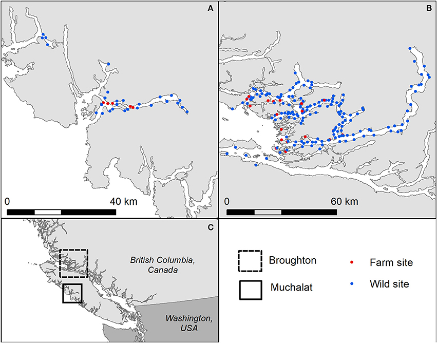
Figure 1. Locations where in situ water temperature measurements and corresponding satellite-derived SST values were obtained for each of the study regions (A) Muchalat Inlet and (B) Broughton Archipelago, with (C) inset map showing administrative boundaries of British Columbia.
Remote Sensing Data
We used level 3 and 4 gridded RS data products in this study. The level 3 “composite” products provide data for variables mapped on uniform space-time grids, usually with some averaging, but do not perform any gap-filling or interpolation. The level 4 “analysis” products are generated by combining several sources of SST data (e.g., satellites, moorings, and ship-based observations) through statistical interpolation and temporal averaging (Martin et al., 2012). These products provide gap-free gridded outputs (Parkinson et al., 2006), and are thought to provide the best available estimates of SST/SSS through data assimilation of available datasets. They provide global coverage and foundational estimates free of diurnal variation (Piolle et al., 2010; Donlon et al., 2012), which are representative of bulk ocean properties; in contrast to the skin or sub-skin estimates provided by the infrared (IR) or microwave satellite sensors (Beggs, 2010; Donlon et al., 2012). Hereafter, the terms “level 3 composite products” and “level 4 analysis products” refer to direct satellite-derived level 3 data, or estimates based on analysis and interpolation of SST/SSS products, respectively. We assessed products that were freely available, widely used, active at the time of study, and effective for coastal data retrieval (Yuan, 2009).
The daily SST level 3 composite product, with 4.6 and 9 km spatial resolution captured via the MODIS (Moderate Resolution Imaging Spectroradiometer)1 sensor on board the Aqua and Terra satellites, and the daily SSS level 3 composite product with 1 degree spatial resolution, captured via SSS sensors on board the Aquarius satellite, were obtained from the Ocean Color website (https://oceancolor.gsfc.nasa.gov/). These daily SST and SSS level 3 composite products are processed and maintained by the NASA Ocean Biology Processing Group. A second daily SSS level 3 composite product from the Soil Moisture and Ocean Salinity (SMOS) satellite of the European Space Agency was acquired, along with daily SST and SSS level 4 analysis products from the Copernicus Marine Environment Monitoring Service of the European Union (CMEMS)2. Table 1 presents the details on the SST and SSS products evaluated, indicating source availability and spatial-temporal resolution.
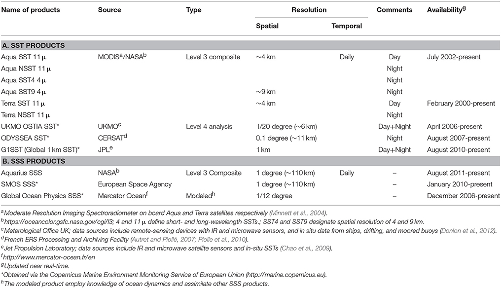
Table 1. Summary of the level 3 composite and level 4 analysis and modeled SST/SSS products evaluated in the present study.
Remotely-sensed data for the corresponding in situ sites (wild and farm) were retrieved from each of the selected SST and SSS products for the study duration (2003–2016), using the raster (Hijmans and van Etten, 2014) and ncdf4 (Pierce, 2012) packages for the R software environment (R Core Team, 2015).
Statistical Comparison
The statistical analyses were performed using Stata (Release 14.1; StataCorp, College Station, TX, USA, 2015) and R version 3.4.1 (R Core Team, 2015) using packages hydroGOF (Zambrano-Bigiarini, 2011) and nlme (Pinheiro et al., 2017). The in situ measurements at 1 m depth were deemed to be the best/most reasonable depth to compare with RS measurements. A number of metrics were used to assess the relationship between products and in situ measurements. First, the difference between the two measurements (value from the overlapping pixel of the RS product minus the in situ measurement, referred to as “bias”) was computed. The mean, standard deviation (SD), and root mean square error (RMSE) of these biases were estimated. Pearson correlation coefficients and concordance correlation coefficients (CCC) between pairs of measurements were also computed. The CCC (Lin, 1989) provides an indication of agreement between two measurements (see Appendix for formula), with values close to 1 indicating very good agreement and values approaching zero reflecting very poor agreement. As in the case of Pearson's correlation, this coefficient is dimensionless; however, CCCs are penalized (adjusted downward) to account for both location- and scale-shifts between measurements, as opposed to simply describing their linear dependence (Pearson correlation).
The spatial footprint of the in situ measurements was point-based, while that of the composite and analysis products was a 2-dimensional pixel that occasionally encompassed multiple in situ points. To evaluate the impact multiple sites within a pixel could have on our metrics we averaged all in situ measurements for a given day, within a pixel, and compared this value to the measurements from the RS products.
We also compared larger temporal windows (weekly and monthly averages), as these better reflect the temporal scales likely to be encountered in aquaculture research. We used index of agreement (d-index) to compare in situ measurements with RS products; this approach has been widely used to assess the performance of hydrologic models (Zambrano-Bigiarini, 2011). The d-index (see Appendix for formula) represents the ratio between RMSE and the potential error between the two measurements (Willmott, 1984; Swierczynska et al., 2016). It is also dimensionless, with a value that ranges from 0 (no agreement at all) to 1 (perfect agreement), and is sensitive to differences between two measurements.
Finally, in order to adjust for differences, a mixed linear regression model was fitted to predict the in situ measurement, using the best performing RS product as the predictor, with sampling site as a random effect (allowing capture of the variability in both the intercept and the coefficient of the predictor), and accounting for autocorrelation between residuals of daily measurements within each site with a first-order autoregressive (AR1) or exponential autocorrelation structure. In order to meet the assumption of linearity, the fitted model also tested functional forms of the predictor using quadratic terms (both as fixed and random effects) and evaluated the fit of the model using both the significance of the additional terms and likelihood ratio test for the nested models. For this analysis, pixels were not included as a random effect due to limited replication at that level.
Results
The total numbers of available daily in situ measurements, from the years 2003–2016, for water temperature and salinity at 1 m depth, were 20,513 (18,093 from farm sites) and 20,038 (18,563 from farm sites), respectively. The mean in situ water temperature and salinity was 10.07°C (range 2.60–21.80) and 23.44 ppt (range 0–33), and varied between the two study areas. The seasonal means for water temperature and salinity were 7.27, 10.44, 13.16, and 8.87°C, and 24.94, 22.43, 22.88, and 23.70 ppt, respectively. Due to many days of cloud cover and the fact that some sites (32, mostly wild surveillance sites) were beyond the satellite coverage area (see Figure 2), a smaller number of matched observations was available for comparison for the SST products. The groups of spatio-temporally (by site and date) matched in situ and SST measurements varied for each of the products (see Table 2).
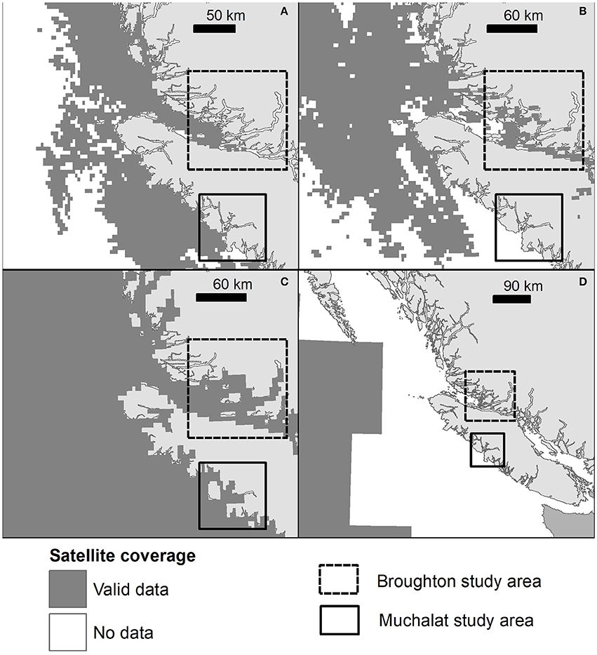
Figure 2. Representation of coverage (for randomly picked dates) of some of the level 3 composite and level 4 analysis SST and SSS product/s for the study sites. (A) Aqua NSST 11 μ, (B) Aqua SST 4 μ, (C) UKMO OSTIA, SST, and (D) Aquarius SSS (right). Maps on the top panel and bottom left are on the same scale.
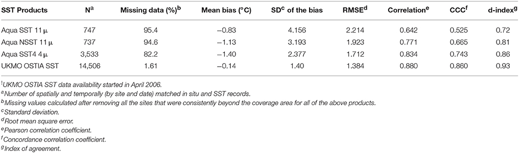
Table 2. Mean bias and correlations between remotely-sensed (level 3 composite and level 4 analysis) SST products and in situ water temperature (at 1 m depth) from 2003 to 2013!.
The mean bias (°C), its SD, and the RMSE for each RS SST product, along with the corresponding Pearson correlation coefficient, CCC, index of agreement (d-index), and proportions of missing data are summarized in Table 2. Of the SST products evaluated, UKMO OSTIA SST (UK Meteorological Office), a level 4 analysis product, had by far the highest retrieval (fewest missing data), the largest correlation coefficient (0.88), CCC (0.86), and d-index (0.93), and the smallest mean and SD for the bias (−0.14 and 1.40, respectively). The plots of the in situ water temperature measurements for the SST products are presented in Figure 3, which indicates a noticeably strong linear relationship, with some dispersion, between in situ water temperature and UKMO OSTIA SST.
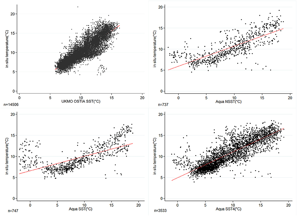
Figure 3. Scatter plots of in situ water temperature (at 1 m depth) to that of each of the satellite-derived SST products (level 3 and level 4) for several sites in the Broughton Archipelago and Muchalet Inlet in coastal British Columbia.
Of the 14,506 spatio-temporally matched in situ measurements with UKMO OSTIA SST, 61% were single measurements within a pixel and day, while 36% of the measurements included two sites within the same pixel and day. The maximum number of sites within a pixel and day was four. After accounting for multiple in situ sites within a pixel/day (n = 11,595), the mean bias and the SD of the mean bias was 0.06 and 1.4°C, respectively, while the correlation coefficient and the CCC were 0.87 and 0.85, respectively.
The correlation coefficients (0.89 and 0.90) and the CCCs (0.87 and 0.88) increased marginally when weekly and monthly averages of UKMO OSTIA SST were compared with in situ measurements, suggesting a marginal increase in similarity when measurements were averaged over a longer period. However, the magnitude of the bias remained unchanged (−0.14), with a slight decrease in variability (SD: 1.30 and 1.22, respectively). Similarly, the correlation coefficients were higher for the subset of the data that included only farm sites, than for those from wild surveillance sites (0.90 compared to 0.83, respectively), as was the case for the CCCs (0.88 and 0.64). This suggests higher variability in the in situ measurements from wild surveillance sites.
The retrieval rates of level 3 composite SST values and their respective statistical comparison with in situ data, using Terra and Aqua satellites with 9 km spatial resolution, were not different from SST values retrieved from Aqua satellites with 4 km spatial resolution (Table 2); thus, summary statistics for those SST products are not presented. Among other level 4 analysis SST products, G1SST (Global 1 km SST) had very limited coverage for our study sites, with many missing values, and the ODYSSEA SST had poor correlation (<0.30) with in situ measurements, so detailed statistics for these products are not presented.
Due to the higher variability of in situ measurements from the wild surveillance sites, the regression model included only measurements from farm sites. A mixed linear regression model with UKMO OSTIA SST as the predictor for in situ measurement estimated an average coefficient of 0.89°C (p < 0.001) for UKMO OSTIA SST across sites that varied between 0.22 and 1.56°C, 95% of the time (Table 3).
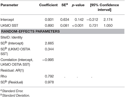
Table 3. Estimates from the linear mixed model, with UKMO OSTIA SST as the predictor, to adjust for in situ measurements (outcome) from coastal British Columbia, with sites as the random intercept and UKMO OSTIA SST as random slope (n = 12,759).
None of the level 3 composite SSS products (Aquarius and SMOS) evaluated provided corresponding values for in situ records, mostly due to their lack of spatial coverage (see Figure 2D) for the study area. The modeled SSS product did have partial coverage for our study area, but the retrieved values had poor correlation (<0.20) with in situ salinity measurements, and detailed statistics for these products are not presented.
Discussion
The main objective of this study was to evaluate whether satellite-derived SST and SSS products provide representations of temperature and salinity in marine ecosystems that would make them suitable as surrogates for environmental variables in aquaculture research. To the best of our knowledge, this is the first study to utilize existing in situ data from fish farms and wild surveillance programs to assess the suitability of RS SST and SSS products.
Our study demonstrated that of the SST products considered, the UKMO OSTIA SST was the most representative of the water temperature profile in coastal BC, Canada. A linear mixed model, after adjusting for autocorrelation, suggested that between-site variation was significant. The UKMO OSTIA SST (a level 4 analysis product) uses satellite SST data provided by international agencies via the Group for High Resolution SST (http://www.ghrsst.org), which include data from both microwave and IR satellite instruments, as well as in situ SST data (Donlon et al., 2012). The SST level 3 composite products we evaluated were often missing information for the study sites, likely due to poor satellite coverage, application of a land mask, or cloud cover (Webster et al., 1996; Guan and Kawamura, 2003). Similar observations for coastal areas have been noted by other studies (Castillo and Lima, 2010; Smit et al., 2013), but the proportion of missing values (80–90%) for some products in our study area was strikingly high, something not reported in previous studies. Nevertheless, the magnitude of bias and correlation between the in situ and RS level 3 composite SST products were comparable to those of other published studies (Castillo and Lima, 2010; Williams et al., 2013).
Our analysis also suggested that the UKMO OSTIA SST measurements were in closer agreement to in situ measurements from farm sites than for wild surveillance sites. The wild surveillance site measurements were captured from shallower waters close to coastlines, and this may have resulted in lower correlation coefficient and CCC values. None of the SSS products evaluated appeared promising for use in aquaculture studies, either due to lack of coverage or very poor correlation with in situ measurements. One of the underlying reasons for this is that, to date, all level 3 composite and modeled SSS products have focused on open ocean rather than coastal applications. The spatial resolution of data from the ESA's Soil Moisture and Ocean Salinity as well as NASA's Aquarius missions are too coarse for coastal and estuarine environments (Figure 2D; Urquhart et al., 2012). In time, finer resolutions, such as that offered by NASA's Soil Moisture Active Passive mission, or novel methods based on selected wavelengths of RS reflectance may provide improved estimates of SSS (Urquhart et al., 2012; Qing et al., 2013).
It should also be noted that certain inherent characteristics of the SST products affect both the retrieval rate and the correlation with in situ measurements. For example, SST products from IR sensors, such as those on MODIS, are sensitive to cloud cover (a primary cause of missing data), while those from microwave sensors are sensitive to precipitation, land contamination, and surface roughness (Donlon et al., 2012). Microwave sensors are limited to much coarser spatial resolution than products derived from IR bands. As a result, IR sensors can retrieve SSTs to within around 1 km of land (dependent on the land mask used), whereas microwave sensors cannot likely retrieve useable SST data within around 75 km of land, far from most aquaculture production areas. Further, IR light is fully attenuated within the top 1 mm of the water column while microwave penetrates only a little deeper (a few mm). In contrast the in situ measurements that we used were typically from a depth of 1 m, so it is possible that we were effectively comparing different segments of the water column when using the level 3 composite SST products.
Similarly, the smaller disagreement between the level 4 analysis product, UKMO OSTIA SST, and in situ measurements may be explained by the fact that the modeled product estimates water temperature through data assimilation from many sources over an integrated surface layer of ~1 m, more closely matching the methods for in situ measurements. Another likely explanation is that in situ measurements at 1 m depth, despite time differences, correlated more strongly because there is less variability (due to diurnal variability, wind, weather, and currents) than at the surface (Donlon et al., 2012). The results may also have been influenced by a temporal mismatch, as instantaneous in situ measurements do not necessarily coincide with the RS data representing either day-time or night-time mean values, introducing a potential source of error and the possibility of aliasing. Additionally, there will inevitably be some mismatch in spatial scale, as the RS and modeled products integrate data over a larger area (1–100 km pixel size) when compared to the point-based in situ observations.
Lastly, in some areas within the study region there were multiple in situ observations recorded within single spatial extents (grid pixels) of the RS composite and analysis products. The aggregation of sites within pixels inevitably led to an overall reduction in the between-site variability and the complete removal of variability among sites within grid pixels when extracting RS data for use at individual sites. This issue may create limitations for researchers when using RS data rather than in situ observations. The extent of the limitation will depend on the application and objectives of the aquatic research, being most significant when capturing among-site variability is important.
The present study reinforces the findings of previous research (Castillo and Lima, 2010; Smit et al., 2013; Williams et al., 2013; Stobart et al., 2015; Wu et al., 2016). The type of SST product used (i.e., composite vs. analysis, satellite, and sensor types), the methods used for capturing in situ measurements, the location of the study area, and the temporal and spatial resolution used for aggregating the RS data are among the key factors associated with a true representation of water temperature profiles in the study area. The evidence suggests significant differences in agreement between satellite products across different regions (Castillo and Lima, 2010; Smit et al., 2013; Williams et al., 2013; Stobart et al., 2015; Wu et al., 2016), which highlights the need for similar studies in other aquaculture areas to assess the suitability of SST products.
Since available in situ water temperature data sources (in our case salmon farms and wild surveillance data) may have substantial numbers of missing values and temporal gaps, the present study provides evidence that satellite data can complement, if not be a substitute for, existing temperature data, though satellite estimates of SSS are not currently suitable for aquaculture applications. This could significantly improve monitoring capabilities relative to in situ observations (Urquhart et al., 2012), as in situ data are not always openly available and often have a lag time (depending on the field collection regimen). The near real-time and free availability of these satellite-based data make them suitable for use in forecast models, in monitoring and surveillance of pathogens, and in creating risk maps for fish health.
Author Contributions
KT, RV, TP, and CR designed the study; TP and CR were instrumental in acquiring in situ data; KT, RV, and JB acquired and processed the remote-sensed data; KT, RV, and HS performed the analysis; KT wrote the first draft of the manuscript and everyone contributed in revising the manuscript.
Funding
This study was funded in the form of a seed grant from the Canada Excellence Research Chair in Aquatic Epidemiology program at the University of Prince Edward Island.
Conflict of Interest Statement
The authors declare that the research was conducted in the absence of any commercial or financial relationships that could be construed as a potential conflict of interest.
Acknowledgments
This study was conducted using the NASA Ocean Color and Copernicus Marine Service Products. We thank the Canada Excellence Research Chair in Aquatic Epidemiology for funding support for this study. Thanks are also due to William Chalmers for editorial assistance with the manuscript. Preliminary findings from this study were presented at the Aquatic Epidemiology Conference held in September 2016 in Oslo, Norway.
Footnotes
1. ^NASA. Goddard Space Flight Center, Ocean Ecology Laboratory, Ocean Biology Processing Group. Moderate-resolution Imaging Spectroradiometer (MODIS) Aqua Sea Surface Temperature Data; 2014 Reprocessing. Greenbelt, MD: NASA OB.DAAC. (Accessed July 3, 2016).
2. ^CMEMS. Copernicus Marine Environment Monitoring Service (European Union). Available online at: http://marine.copernicus.eu
References
Altizer, S., Dobson, A., Hosseini, P., Hudson, P., Pascual, M., and Rohani, P. (2006). Seasonality and the dynamics of infectious diseases. Ecol. Lett. 9, 467–484. doi: 10.1111/j.1461-0248.2005.00879.x
Arriagada, G., Vanderstichel, R., Stryhn, H., Milligan, B., and Revie, C. (2016). Evaluation of water salinity effects on the sea lice Lepeophtheirus salmonis found on farmed Atlantic salmon in Muchalat Inlet, British Columbia, Canada. Aquaculture 464, 554–563. doi: 10.1016/j.aquaculture.2016.08.002
Autret, E., and Piollé, J. (2007). ODYSSEA Global SST Analysis-User manual. CERSAT–IFREMER MERSEA-WP02-IFRSTR-001-1A.
BAMP (2010). Broughton Archipelago Monitoring Plan. Available online at: http://bamp.ca
Beggs, H. M. (2010). “Use of TIR from space in operational systems,” in Oceanography from Space, eds V. Barale, J. F. R. Gower, and L. Alberotanza (London: Springer), 249–271.
Bojinski, S., Verstraete, M., Peterson, T. C., Richter, C., Simmons, A., and Zemp, M. (2014). The concept of essential climate variables in support of climate research, applications, and policy. Bull. Am. Meteorol. Soc. 95, 1431–1443. doi: 10.1175/BAMS-D-13-00047.1
Bowden, T. J. (2008). Modulation of the immune system of fish by their environment. Fish Shellfish Immunol. 25, 373–383. doi: 10.1016/j.fsi.2008.03.017
Brewer-Dalton, K., Page, F. H., Chandler, P., and Ratsimandresy, A. (2015). Oceanographic Conditions of Salmon Farming Areas with Attention to Those Factors That May Influence the Biology and Ecology of Sea Lice, Lepeophtherius salmonis and Caligus spp., and Their Control. DFO Can. Sci. Advis. Sec. Res. Doc. 2014/048. vi + 47.
Casey, K. S., Brandon, T. B., Cornillon, P., and Evans, R. (2010). “The past, present, and future of the AVHRR Pathfinder SST program,” in Oceanography From Space, eds V. Barale, J. Gower, and L. Alberotanza (Dordrecht: Springer), 273–287.
Castillo, K. D., and Lima, F. P. (2010). Comparison of in situ and satellite-derived (MODIS-Aqua/Terra) methods for assessing temperatures on coral reefs. Limnol. Oceanogr. Methods 8, 107–117. doi: 10.4319/lom.2010.8.0107
Chao, Y., Li, Z., Farrara, J. D., and Hung, P. (2009). Blending sea surface temperatures from multiple satellites and in situ observations for coastal oceans. J. Atmos. Ocean Technol. 26, 1415–1426. doi: 10.1175/2009JTECHO592.1
Donlon, C. J., Martin, M., Stark, J., Roberts-Jones, J., Fiedler, E., and Wimmer, W. (2012). The operational sea surface temperature and sea ice analysis (OSTIA) system. Remote Sens. Environ. 116, 140–158. doi: 10.1016/j.rse.2010.10.017
Ferreira, J. G., Aguilar-Manjarrez, J., Bacher, C., Black, K., Dong, S., Grant, J., et al. (2012). “Progressing aquaculture through virtual technology and decision-support tools for novel management,” in Global Conference on Aquaculture 2010. (Phuket).
Filgueira, R., Grant, J., Stuart, R., and Brown, M. (2013). Ecosystem modelling for ecosystem-based management of bivalve aquaculture sites in data-poor environments. Aquac. Environ. Interact. 4, 117–133. doi: 10.3354/aei00078
Findlay, R. H., and Watling, L. (1997). Prediction of benthic impact for salmon net-pens based on the balance of benthic oxygen supply and demand. Mar. Ecol. Prog. Ser. 155, 147–157. doi: 10.3354/meps155147
Foreman, M. G. G., Chandler, P. C., Stucchi, D. J., Garver, K. A., Guo, M., Morrison, J., et al. (2015). The Ability of Hydrodynamic Models to Inform Decisions on the Siting and Management of Aquaculture Facilities in British Columbia. DFO Can. Sci. Advis. Sec. Res. Doc. 2015/005. vii + 49.
GCOS (2015). Status of the Global Observing System for Climate. Geneva: World Meteorological Organization.
Groner, M. L., McEwan, G. F., Rees, E. E., Gettinby, G., and Revie, C. W. (2016). Quantifying the influence of salinity and temperature on the population dynamics of a marine ectoparasite. Can. J. Fish. Aquat. Sci. 73, 1281–1291. doi: 10.1139/cjfas-2015-0444
Guan, L., and Kawamura, H. (2003). SST availabilities of satellite infrared and microwave measurements. J. Oceanogr. 59, 201–209. doi: 10.1023/A:1025543305658
Handeland, S. O., Imsland, A. K., and Stefansson, S. O. (2008). The effect of temperature and fish size on growth, feed intake, food conversion efficiency and stomach evacuation rate of Atlantic salmon post-smolts. Aquaculture 283, 36–42. doi: 10.1016/j.aquaculture.2008.06.042
Harvell, C. D., Kim, K., Burkholder, J. M., Colwell, R. R., Epstein, P. R., Grimes, D. J., et al. (1999). Emerging marine diseases–climate links and anthropogenic factors. Science 285, 1505–1510. doi: 10.1126/science.285.5433.1505
Hijmans, R. J., and van Etten, J. (2014). Raster: Geographic Data Analysis and Modeling. R package version 2, 15. Available online at: http://CRAN.R-project.org/package=raster
Hollmann, R., Merchant, C., Saunders, R., Downy, C., Buchwitz, M., Cazenave, A., et al. (2013). The ESA climate change initiative: satellite data records for essential climate variables. Bull. Am. Meteorol. Soc. 94, 1541–1552. doi: 10.1175/BAMS-D-11-00254.1
Horning, N., Robinson, J., Sterling, E., Turner, W., and Spector, S. (2010). Remote Sensing for Ecology and Conservation. New York, NY: Oxford University Press.
Ishii, M., Shouji, A., Sugimoto, S., and Matsumoto, T. (2005). Objective analyses of sea-surface temperature and marine meteorological variables for the 20th century using ICOADS and the Kobe collection. Int. J. Climatol. 25, 865–879. doi: 10.1002/joc.1169
Jones, S., and Beamish, R. (2011). Salmon Lice: An Integrated Approach to Understanding Parasite Abundance and Distribution. Oxford, UK: John Wiley & Sons.
Jones, S., and Johnson, S. (2015). Sea lice Monitoring and Non-Chemical Measures A: Biology of Sea Lice, Lepeophtheirus salmonis and Caligus spp., in Western and Eastern Canada. DFO Can. Sci. Advis. Sec. Res. Doc. 2014/019 Pacific Region. Pacific Biological Station. Fisheries and Oceans Canada.
Lagerloef, G., Colomb, F. R., Le Vine, D., Wentz, F., Yueh, S., Ruf, C., et al. (2008). The Aquarius/SAC-D mission: designed to meet the salinity remote-sensing challenge. Oceanography 21, 68–81. doi: 10.5670/oceanog.2008.68
Lagerloef, G. S., Swift, C. T., and LeVine, D. M. (1995). Sea surface salinity: the next remote sensing challenge. Oceanography 8, 44–50. doi: 10.5670/oceanog.1995.17
Lin, L. I. (1989). A concordance correlation coefficient to evaluate reproducibility. Biometrics 45, 255–268.
Le Traon, P.-Y., Antoine, D., Bentamy, A., Bonekamp, H., Breivik, L., Chapron, B., et al. (2015). Use of satellite observations for operational oceanography: recent achievements and future prospects. J. Oper. Oceanogr. 8, s12–s27. doi: 10.1080/1755876X.2015.1022050
Malick, M. J., and Cox, S. P. (2016). Regional-scale declines in productivity of pink and chum salmon stocks in Western North America. PLoS ONE 11:e0146009. doi: 10.1371/journal.pone.0146009
Marcogliese, D. J. (2001). Implications of climate change for parasitism of animals in the aquatic environment. Can. J. Zool. 79, 1331–1352. doi: 10.1139/z01-067
Martin, M., Dash, P., Ignatov, A., Banzon, V., Beggs, H., Brasnett, B., et al. (2012). Group for High Resolution Sea Surface temperature (GHRSST) analysis fields inter-comparisons. Part 1: A GHRSST multi-product ensemble (GMPE). Deep Sea Res. Part 2 Top. Stud. Oceanogr. 77, 21–30. doi: 10.1016/j.dsr2.2012.04.013
Maynard, J., van Hooidonk, R., Harvell, C. D., Eakin, C. M., Liu, G., Willis, B. L., et al. (2016). Improving marine disease surveillance through sea temperature monitoring, outlooks and projections. Philos. Trans. R. Soc. B. 371:20150208. doi: 10.1098/rstb.2015.0208
Minnett, P. J., Brown, O. B., Evans, R. H., Key, E. L., Kearns, E. J., Kilpatrick, K., et al. (2004). “Sea-surface temperature measurements from the Moderate-Resolution Imaging Spectroradiometer (MODIS) on Aqua and Terra,” in Geoscience and Remote Sensing Symposium, (2004). IGARSS'04. Proceedings, 2004 IEEE International, (Anchorage, AK). 4576–4579.
Mueter, F. J., Peterman, R. M., and Pyper, B. J. (2002). Opposite effects of ocean temperature on survival rates of 120 stocks of Pacific salmon (Oncorhynchus spp.) in northern and southern areas. Can. J. Fish. Aquat. Sci. 59, 456–463. doi: 10.1139/f02-020
Parkinson, C., Ward, A., and King, M. (2006). Earth Science Reference Handbook: A Guide to NASA's Earth Science Program and Earth Observing Satellite Missions. Washington, DC: National Aeronautics and Space Administration.
Pierce, D. (2012). ncdf4: Interface to Unidata netCDF (version 4 or earlier) Format Data Files. R package. Available online at: http://CRAN.R-project.org/package=ncdf4
Pinheiro, J., Bates, D., DebRoy, S., Sarkar, D., Heisterkamp, S., Van Willigen, B., et al. (2017). Package ‘nlme’. Linear and Nonlinear Mixed Effects Models. R package version 3.1-131.1. Available online at: https://CRAN.R-project.org/package=nlme
Piolle, J.-F., Autret, E., Arino, O., Robinson, I. S., and Le Borgne, P. (2010). “Medspiration: toward the sustained delivery of satellite sst products and services over regional seas,” in Proceedings of ESA Living Planet Symposium (Bergen).
Qing, S., Zhang, J., Cui, T., and Bao, Y. (2013). Retrieval of sea surface salinity with MERIS and MODIS data in the Bohai Sea. Remote Sens. Environ. 136, 117–125. doi: 10.1016/j.rse.2013.04.016
R Core Team (2015). R: A Language and Environment for Statistical Computing. Vienna: R Foundation for Statistical Computing. Available online at: https://cran.r-project.org
Rees, E., St-Hilaire, S., Jones, S., Krkošek, M., DeDominicis, S., Foreman, M., et al. (2015). Spatial patterns of sea lice infection among wild and captive salmon in western Canada. Landsc. Ecol. 30, 989–1004. doi: 10.1007/s10980-015-0188-2
Rogers, L. A., Peacock, S. J., McKenzie, P., DeDominicis, S., Jones, S. R., Chandler, P., et al. (2013). Modeling parasite dynamics on farmed salmon for precautionary conservation management of wild salmon. PLoS ONE 8:e60096. doi: 10.1371/journal.pone.0060096
Santos, A. M. P. (2000). Fisheries oceanography using satellite and airborne remote sensing methods: a review. Fish. Res. 49, 1–20. doi: 10.1016/S0165-7836(00)00201-0
Savtchenko, A., Ouzounov, D., Ahmad, S., Acker, J., Leptoukh, G., Koziana, J., et al. (2004). Terra and Aqua MODIS products available from NASA GES DAAC. Adv. Space Res. 34, 710–714. doi: 10.1016/j.asr.2004.03.012
Smit, A. J., Roberts, M., Anderson, R. J., Dufois, F., Dudley, S. F., Bornman, T. G., et al. (2013). A coastal seawater temperature dataset for biogeographical studies: large biases between in situ and remotely-sensed data sets around the coast of South Africa. PLoS ONE 8:e81944. doi: 10.1371/journal.pone.0081944
Stien, A., Bjørn, P. A., Heuch, P. A., and Elston, D. A. (2005). Population dynamics of salmon lice Lepeophtheirus salmonis on Atlantic salmon and sea trout. Mar. Ecol. Prog. Ser. 290, 263–275. doi: 10.3354/meps290263
Stobart, B., Mayfield, S., Mundy, C., Hobday, A., and Hartog, J. (2015). Comparison of in situ and satellite sea surface-temperature data from South Australia and Tasmania: how reliable are satellite data as a proxy for coastal temperatures in temperate southern Australia? Mar. Freshw. Res. 67, 612–625. doi: 10.1071/MF14340
Stucchi, D. J., Guo, M., Foreman, M. G., Czajko, P., Galbraith, M., Mackas, D. L., et al. (2011). “Modeling sea lice production and concentrations in the Broughton Archipelago, British Columbia,” in Salmon Lice: An Integrated Approach to Understanding Parasite Abundance and Distribution, eds S. Jones and R. Beamish (Chichester: John Wiley & Sons, Ltd.), 117–150.
Swierczynska, M., Mizinski, B., and Niedzielski, T. (2016). Comparison of predictive skills offered by prognocean, prognocean plus and myocean real-time sea level forecasting systems. Ocean Eng. 113, 44–56. doi: 10.1016/j.oceaneng.2015.12.023
Urquhart, E. A., Zaitchik, B. F., Hoffman, M. J., Guikema, S. D., and Geiger, E. F. (2012). Remotely sensed estimates of surface salinity in the Chesapeake Bay: a statistical approach. Remote Sens. Environ. 123, 522–531. doi: 10.1016/j.rse.2012.04.008
Webster, P. J., Clayson, C. A., and Curry, J. A. (1996). Clouds, radiation, and the diurnal cycle of sea surface temperature in the tropical western Pacific. J. Clim. 9, 1712–1730.
Williams, G., Sapoznik, M., Ocampo-Reinaldo, M., Solis, M., Narvarte, M., González, R., et al. (2010). Comparison of AVHRR and SeaWiFS imagery with fishing activity and in situ data in San Matías Gulf, Argentina. Int. J. Remote Sens. 31, 4531–4542. doi: 10.1080/01431161.2010.485218
Williams, G. N., Dogliotti, A., Zaidman, P., Solis, M., Narvarte, M., Gonzalez, R., et al. (2013). Assessment of remotely-sensed sea-surface temperature and chlorophyll-a concentration in San Matías Gulf (Patagonia, Argentina). Cont. Shelf Res. 52, 159–171. doi: 10.1016/j.csr.2012.08.014
Willmott, C. J. (1984). “On the evaluation of model performance in physical geography,” in Spatial Statistics and Models, eds G. L. Gaile and C. J. Willmott (Dordrecht: Springer), 443–460. doi: 10.1007/978-94-017-3048-8_23
Wu, Y., Sheng, J., Senciall, D., and Tang, C. (2016). A comparative study of satellite-based operational analyses and ship-based in-situ observations of sea surface temperatures over the eastern Canadian shelf. Satell Oceanogr Meteorol. 1, 1–10. doi: 10.18063/SOM.2016.01.003
Yuan, D. (2009). Science Focus: Sea Surface Temperature Measurements of the MODIS and AIRS Instruments Onboard of Aqua Satellite. Available online at: https://disc.gsfc.nasa.gov/oceans/science-focus/modis/MODIS_and_AIRS_SST_comp.html
Zagaglia, C. R., Lorenzzetti, J. A., and Stech, J. L. (2004). Remote sensing data and longline catches of yellowfin tuna (Thunnus albacares) in the equatorial Atlantic. Remote Sens. Environ. 93, 267–281. doi: 10.1016/j.rse.2004.07.015
Zambrano-Bigiarini, M. (2011). hydroGOF: Goodness-of-fit functions for Comparison of Simulated and Observed Hydrological time Series. R package version 0.3-2. Available online at: http://CRAN.R-project.org/package=hydroGOF
Appendix
1. Concordance correlation coefficient: The concordance correlation coefficient (Lin, 1989), between two vectors (x and y) of length N is computed as
where the means, the variances and the covariance is respectively computed as:
(a) the means
(b) the variances
(c) and the covariance
2. Index of agreement: The index of agreement (Willmott, 1984), d-index, between two vectors (x and y) of length N is computed as
Keywords: sea surface temperature, sea surface salinity, in situ, satellite remote sensing, MODIS, aquaculture
Citation: Thakur KK, Vanderstichel R, Barrell J, Stryhn H, Patanasatienkul T and Revie CW (2018) Comparison of Remotely-Sensed Sea Surface Temperature and Salinity Products With in Situ Measurements From British Columbia, Canada. Front. Mar. Sci. 5:121. doi: 10.3389/fmars.2018.00121
Received: 15 November 2017; Accepted: 21 March 2018;
Published: 06 April 2018.
Edited by:
Nesar Ahmed, University of Manitoba, CanadaReviewed by:
Yi Zhou, Institute of Oceanology (CAS), ChinaPedro M. Costa, Universidade Nova de Lisboa, Portugal
Copyright © 2018 Thakur, Vanderstichel, Barrell, Stryhn, Patanasatienkul and Revie. This is an open-access article distributed under the terms of the Creative Commons Attribution License (CC BY). The use, distribution or reproduction in other forums is permitted, provided the original author(s) and the copyright owner are credited and that the original publication in this journal is cited, in accordance with accepted academic practice. No use, distribution or reproduction is permitted which does not comply with these terms.
*Correspondence: Krishna K. Thakur, a3RoYWt1ckB1cGVpLmNh