 Mattias R. Cape1*
 Maria Vernet2
 Erin C. Pettit3
 Julia Wellner4Martin Truffer3Garrett Akie5Eugene Domack6†
 Amy Leventer7
 Craig R. Smith8
 Bruce A. Huber9
- 1School of Oceanography, University of Washington, Seattle, WA, United States
- 2Integrative Oceanography Division, Scripps Institution of Oceanography, University of California, San Diego, La Jolla, CA, United States
- 3Geophysical Institute, University of Alaska Fairbanks, Fairbanks, AK, United States
- 4Department of Earth and Atmospheric Sciences, University of Houston, Houston, TX, United States
- 5Hydrological Science and Engineering Program, Colorado School of Mines, Golden, CO, United States
- 6College of Marine Science, University of South Florida, St. Petersburg, FL, United States
- 7Department of Geology, Colgate University, Hamilton, NY, United States
- 8School of Ocean and Earth Science and Technology, University of Hawai’i at Mānoa, Honolulu, HI, United States
- 9Lamont-Doherty Earth Observatory of Columbia University, Palisades, NY, United States
Warming along the Antarctic Peninsula has led to an increase in the export of glacial meltwater to the coastal ocean. While observations to date suggest that this freshwater export acts as an important forcing on the marine ecosystem, the processes linking ice–ocean interactions to lower trophic-level growth, particularly in coastal bays and fjords, are poorly understood. Here, we identify salient hydrographic features in Barilari Bay, a west Antarctic Peninsula fjord influenced by warm modified Upper Circumpolar Deep Water. In this fjord, interactions between the glaciers and ocean act as a control on coastal circulation, contributing to the redistribution of water masses in an upwelling plume and a vertical flux of nutrients toward the euphotic zone. This nutrient-rich plume, containing glacial meltwater but primarily composed of ambient ocean waters including modified Upper Circumpolar Deep Water, spreads through the fjord as a 150-m thick layer in the upper water column. The combination of meltwater-driven stratification, long residence time of the surface plume owing to weak circulation, and nutrient enrichment promotes phytoplankton growth within the fjord, as evidenced by shallow phytoplankton blooms and concomitant nutrient drawdown at the fjord mouth in late February. Gradients in meltwater distributions are further paralleled by gradients in phytoplankton and benthic community composition. While glacial meltwater export and upwelling of ambient waters in this way contribute to elevated primary and secondary productivity, subsurface nutrient enhancement of glacially modified ocean waters suggests that a portion of these macronutrients, as well any iron upwelled or input in meltwater, are exported to the continental shelf. Sustained atmospheric warming in the coming decades, contributing to greater runoff, would invigorate the marine circulation with consequences for glacier dynamics and biogeochemical cycling within the fjord. We conclude that ice–ocean interactions along the Antarctic Peninsula margins act as an important control on coastal marine ecosystems, with repercussions for carbon cycling along the west Antarctic Peninsula shelf as a whole.
Introduction
Since 1950, glaciers along the western Antarctic Peninsula (WAP) have undergone rapid change (Cook et al., 2005, 2016), with thinning and acceleration leading to an ice mass loss of 20 Gt yr-1 between 1992 and 2011, a corresponding increase in the export of glacial ice and freshwater to coastal regions, and a contribution to sea-level rise of 0.16 ± 0.06 mm yr-1 (Pritchard and Vaughan, 2007; Rye et al., 2014; Schannwell et al., 2016). The southerly progression of ice-shelf collapse and glacier acceleration along the eastern AP have been attributed to warming of air temperatures (Cook et al., 2005), reflected in the migration of the -9°C mean annual temperature isotherm (Vaughan and Doake, 1996; Cook and Vaughan, 2010). In contrast, southerly glaciers along the western AP have instead experience greater loss than in the north (Cook et al., 2016).
Near-simultaneous mass loss amongst tidewater glaciers of the southern Antarctic Peninsula in the absence of clear atmospheric forcing suggests the ocean may have played a role (Jakobsson et al., 2011; Rignot et al., 2013; Wouters et al., 2015; Cook et al., 2016). The peninsula, and specifically its southern reaches, is influenced by Circumpolar Deep Water, a warm (1–2°C) water mass transported in the Antarctic Circumpolar Current (Figures 1A,B) (Klinck, 1998; Jenkins and Jacobs, 2008; Martinson et al., 2008; Moffat et al., 2008). The upper branch of upper circumpolar deep water is usually found between 200 and 400 m, and can be advected across the Antarctic Slope Front and deep (>500 m) continental shelf as a result of eddy activity; it is then transformed into modified Upper Circumpolar Deep Water (mUCDW) as a result of mixing and cooling (Martinson et al., 2008; Martinson and McKee, 2012; Stewart and Thompson, 2015; Couto et al., 2017). Hydrographic sampling has documented the presence of mUCDW along the continental shelf as far north as Flandres Bay, inshore of Anvers Island at 63.3°S (Figure 1A) (Cook et al., 2016), and noted shoaling and warming of this water mass over the continental shelf over the past 50 years (Martinson et al., 2008; Schmidtko et al., 2014; Couto et al., 2017; Spence et al., 2017). Presence of warm mUCDW along the inner shelf suggests that ocean-driven melting has contributed to changing ice sheet dynamics over the Southern WAP (Wouters et al., 2015; Cook et al., 2016).
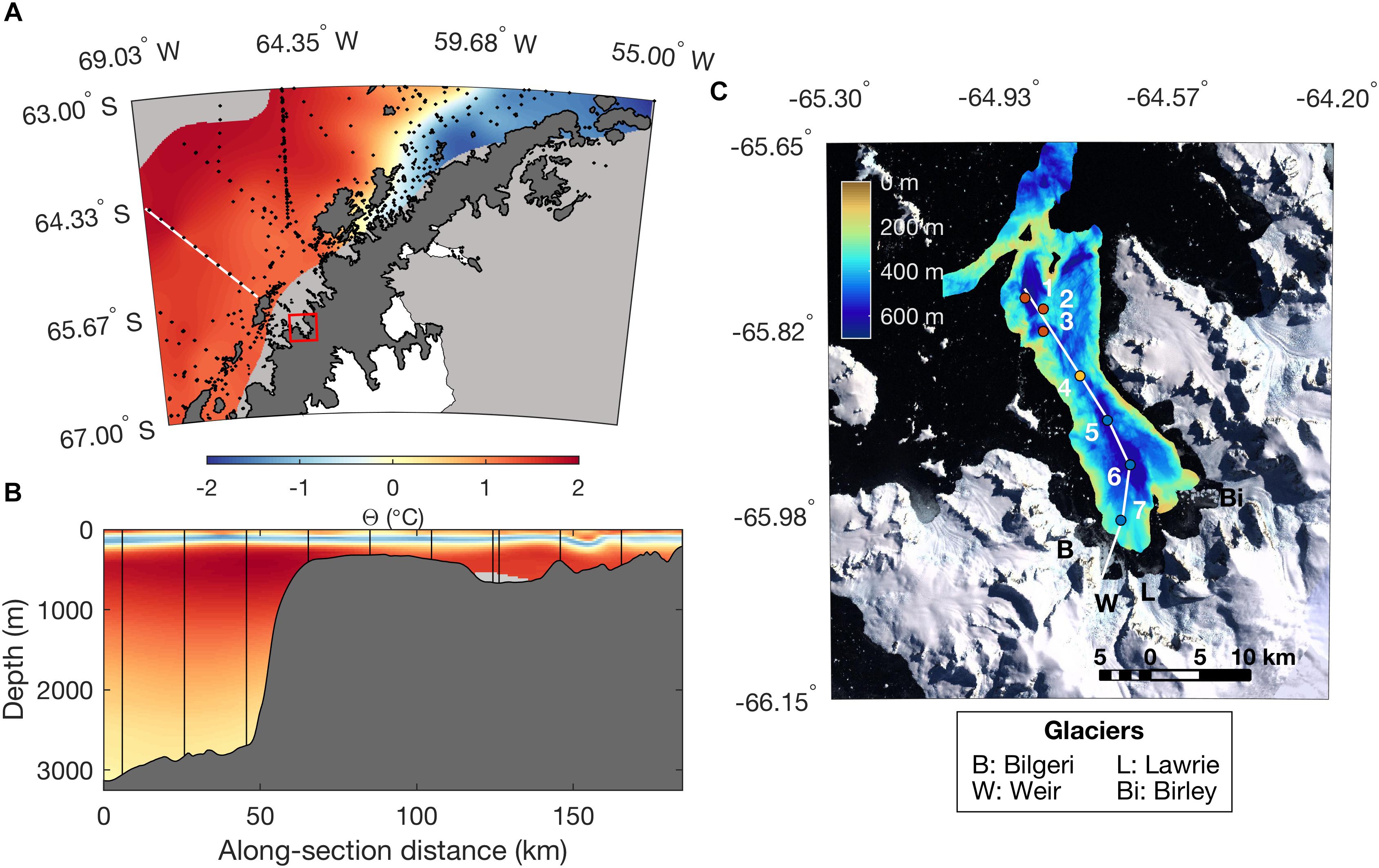
Figure 1. Map of the study area depicting (A) the Antarctic Peninsula. Black points correspond to hydrographic stations contained in the World Ocean Database. Color shading depicts ocean temperature along the σ𝜃 = 27.75 kg m-3 isopycnal, corresponding to the core of the mUCDW layer on the WAP continental shelf. The white line, corresponding to the 500-line of the Palmer LTER grid, indicates the cross-shelf section shown in (B), and the red box indicates the location of Barilari Bay, shown in (C). The Antarctic coastline is derived from MOA2009 (Haran et al., 2014). (B) Cross-shelf section of temperature along the line shown in (A). Black vertical lines indicate the location of hydrographic stations. Bathymetry is indicated by dark gray shading. (C) Landsat image of Barilari Bay from the Landsat Image Mosaic of Antarctica (Bindschadler et al., 2008), showing location of occupied hydrographic stations. Stations are color-coded by location for references in the remaining figures, including reference stations (red), mouth (yellow), and inner fjord (blue). Colored shading indicates processed bathymetry collected during NPB1001. Letters indicate the location of marine-terminating glaciers flowing into Barilari Bay, and the white line the along-fjord section shown in Figure 3.
While the ocean may have a profound impact on the ice sheet, release of freshwater into the coastal ocean also serves as an important forcing on the polar marine environment. Freshwater exported along the WAP enters the ocean primarily at the head of bays and fjords from marine-terminating (tidewater) glaciers and ice shelves, grounded well below the ocean surface (Powell and Domack, 2002). In these systems, freshwater is released at depth as submarine melt (the result of ocean melting of the glacial margin) and subglacial discharge (basal or surface melt routed beneath the ice sheet). Icebergs constitute an additional submarine meltwater source which can significantly contribute to local and regional freshwater export. Distributed export of freshwater acts as a driver for circulation, leading to the formation of turbulent, buoyant plumes at the glacial margins (Jenkins, 1999; Truffer and Motyka, 2016). This buoyant plume entrains ambient ocean waters vertically, with mixing between oceanic and glacial waters leading to the formation of a new, glacially modified water mass (GMW) which acts as the primary vehicle of transport of meltwater in the marine environment. This water mass can be distributed over a significant volume of the upper water column as a result of interactions between the rising plume and ambient stratification (Jacobs et al., 1979; Jenkins and Jacobs, 2008; Straneo et al., 2011). The vertical redistribution of ocean water due to meltwater intrusion along the glacial margins contributes to modification of physical and chemical characteristics of the upper ocean, as previously observed along the Antarctic Peninsula at the margins of George V ice shelf (Jenkins and Jacobs, 2008). These modified coastal waters are ultimately exported to the open ocean.
Previous studies along the Antarctic coast suggest that glacial meltwater inputs may act as an important physical forcing on carbon cycling and coastal marine communities. Productivity in near-shore, glacier-influenced waters of Marguerite Bay, Arthur Harbor, and Potter Cove exceeds that of continental shelf waters (Schloss et al., 2002; Clarke, 2008). These patterns are hypothesized to result from the input of macronutrients and iron as a result of upwelling of deep mUCDW and iron-rich meltwater export in these coastal systems (Prézelin et al., 2000, 2004; Dinniman et al., 2012; Gerringa et al., 2012; Hodson et al., 2017), as well as the concomitant meltwater-induced stabilization of the water column (Mitchell et al., 1991). High megabenthic abundance in WAP fjords compared to the shelf also suggests a link between glacial inputs and increased carbon export (Grange and Smith, 2013), a relationship noted in fjord systems globally (Smith et al., 2015). Finally, AP fjords and bays have been identified as hotspots of secondary productivity, with large aggregations of krill and feeding whales in fjords potentially taking advantage of meltwater-enhanced phytoplankton productivity and biomass (Thiele et al., 2004; Ducklow et al., 2007; Nowacek et al., 2011; Ware et al., 2011; Espinasse et al., 2012). Collectively, these observations are consistent with findings of surveys of Arctic and sub-Arctic glacial fjords (Lydersen et al., 2014; O’Neel et al., 2015; Pettit et al., 2015a; Arimitsu et al., 2016), where systems influenced by glacial meltwater tend to be associated with high primary and secondary productivity and can be disproportionately important as habitat, refuge, and feeding grounds for higher trophic levels.
While influencing near-shore waters, glacial inputs are also thought to play an important role in ecosystem dynamics farther offshore across the WAP continental shelf. Glacial meltwater has emerged as potentially significant source of iron to the marine environment (Death et al., 2014; Annett et al., 2017; Hodson et al., 2017), a limiting micronutrient in the Southern Ocean (Martin et al., 1990). Field studies have noted elevated glacial meltwater content coincident with high standing stocks of dissolved iron along the southern Antarctic Peninsula continental shelf (Weston et al., 2013; Annett et al., 2015; Bown et al., 2018). Most recently, investigation of sources and sinks of iron across the WAP shelf identified glacial meltwater as a critical component of WAP continental-shelf iron budgets (Annett et al., 2017). Considering the carbon cycling ramifications of iron export, these observations also lend credence to the hypothesis that glacial meltwater acts as an important control on phytoplankton production and community composition in this region (Dierssen et al., 2002; Vernet et al., 2008; Meredith et al., 2013).
Along the WAP, long-term monitoring of freshwater composition of the upper ocean at the Rothera Oceanographic and Biological Time Series in northern Marguerite Bay has noted changes in meteoric (a term encompassing precipitation and glacial melt) content of the upper water column over the 21st century associated with variability in atmospheric forcing (Meredith et al., 2010). Sampling along the open WAP continental shelf has provided further insight into spatial gradients in meltwater distribution and concentration (Meredith et al., 2013, 2017). Previous studies have also detailed pathways of glacial meltwater in the Amundsen Sea and their contributions to freshening of the Ross Sea (Nakayama et al., 2014), and demonstrated that the input of glacially derived iron into the Amundsen Sea, e.g., in the Pine Island area, can serve to support the high rates of primary productivity observed in the region (Gerringa et al., 2012; Planquette et al., 2013; Sherrell et al., 2015). However, despite a growing body of literature identifying glacial meltwater as a critical forcing on the WAP marine ecosystem, observations near these glacial sources are lacking, with only a handful of studies to date exploring interactions between ice and ocean in the coastal bays and fjords of the WAP, where a large fraction of the glacial meltwater enters the ocean (Jenkins and Jacobs, 2008). Understanding ice–ocean exchanges is nevertheless critical, given that they determine the initial volume of exported submarine meltwater, the physical and chemical properties of glacially modified waters, their distribution in the vertical and horizontal, as well as the timing of GMW export to the continental shelf (Straneo and Cenedese, 2015). These processes act as a primary determinant for the physical and biogeochemical impact of glacial meltwater input farther downstream along the continental shelf and the large-scale ocean.
In this study, we provide insight into glacier–ocean interactions, as well as their impact on coastal biogeochemistry, by examining physical, chemical, and biological properties of Barilari Bay, a coastal embayment into which five tidewater glaciers terminate. Using hydrographic profiles collected during a synoptic survey, we first map the distribution of water masses, identifying glacially modified waters and their biogeochemical properties. We examine model estimates of glacial discharge into Barilari Bay using a high-resolution mass-balance model and compare these with estimates of meltwater content of coastal waters derived from hydrographic sampling to estimate residence time of meltwater in this system. Finally, we examine the characteristics of the phytoplankton community, putting these observations in context by analyzing patterns of sedimentation and benthic community composition in order to better constrain long-term patterns of benthopelagic coupling. We find that mUCDW is present throughout the glacial fjord, contributing to melt of the glacier termini and the export of glacial meltwater in the top 150 m of the water column. Given low macro-nutrient standing stocks present in glacial ice, nutrient enrichment of this upper fjord layer relative to waters outside the fjord further suggests that nutrient-rich mUCDW, upwelled as a result of freshwater input at the glacial margin, acts as the source of nutrients to this glacially modified layer. This vertical nutrient flux likely contributes to elevated phytoplankton biomass and primary production in this system. In detailing export pathways of these nutrient-enriched water to the continental shelf, we further shed light on the connection between ice–ocean interaction and marine ecosystem processes on the WAP shelf.
Materials and Methods
Study Site
Barilari Bay is a glacier-marine fjord in Graham Land, Antarctic Peninsula located at 65.97°S and 64.65°W (Figure 1C). Although shorter and wider than typical fjords in the Arctic, bays along the Antarctic Peninsula such as Barilari have been previously designated as fjords in the literature because they are glacially carved estuaries with U-shaped cross sections (e.g., Domack and Ishman, 1993; Grange and Smith, 2013). We therefore use the terms fjord and bay interchangeably to refer to Barilari Bay in the remainder of this study.
Barilari is exposed to a cold climate relative to the more subpolar northern AP, with summer atmospheric temperature remaining on average below 0°C (Supplementary Figure 1). The bay has a U-shaped glacial trough of 580 m average depth, is 22 km long and 10 km wide at its narrowest point, with three basins separated by deep (>300 m) sills (Figure 1C). The basins define a glacier-proximal inner fjord, a middle distal fjord and an outer, oceanic fjord. Four glaciers deliver ice to the inner terminal fjord, including Bilgeri, Weir, Lawrie, and Birley (Figures 1C, 2).
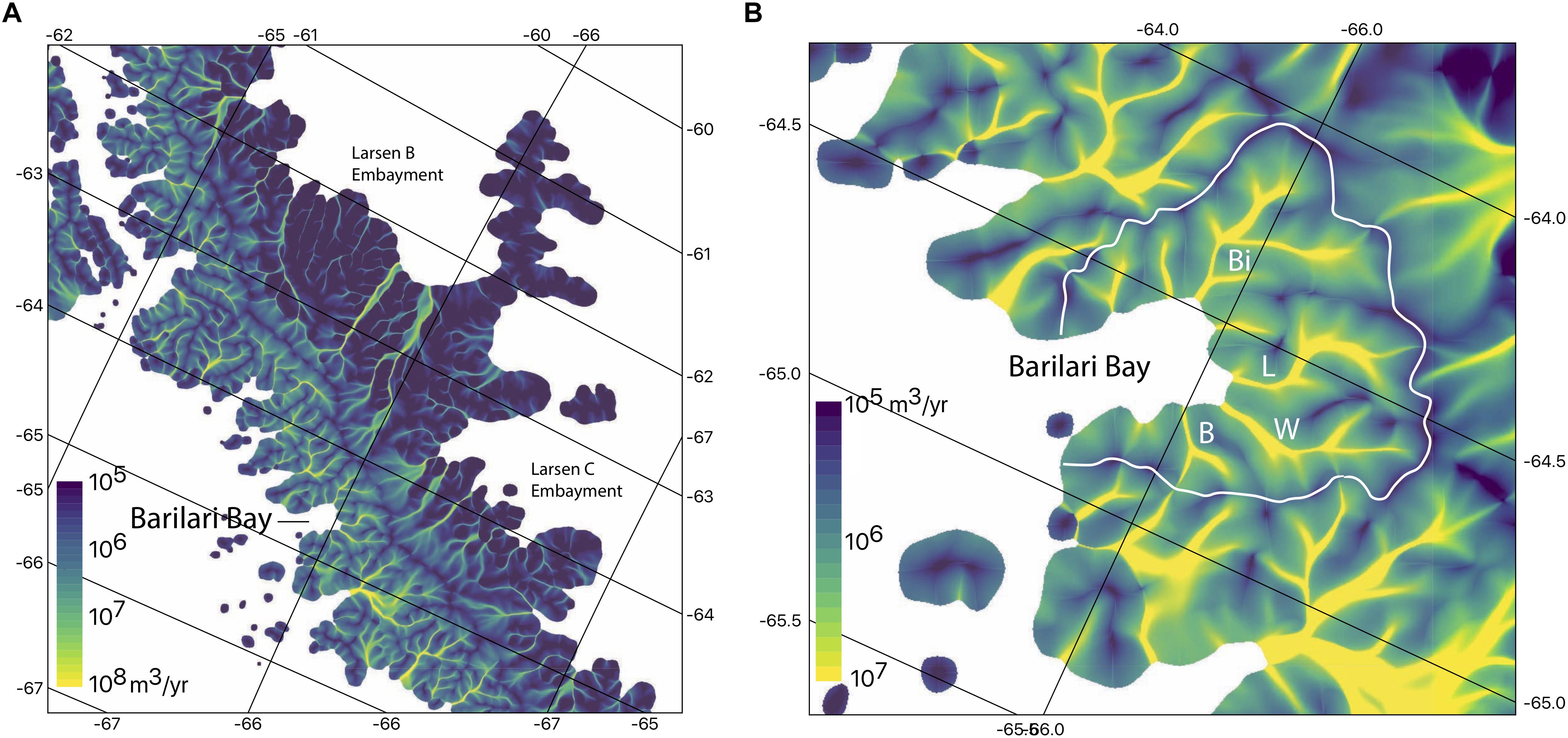
Figure 2. Estimated flux of ice from glacier catchments in Barilari Bay. Flux in each grid cell is calculated as a mean over the 100 m grid size. The coastline is based on the MOA 2009. (A) The flux over a wider region that includes both sides of the peninsula and shows the location of Barilari Bay to the Larsen B and C embayments. (B) Barilari Bay identifying the same four glaciers as in Figure 1C. White line delineates the ice divides separating drainage basins.
Sampling Scheme
Barilari Bay stations were occupied between January 22 and 25 as well as between February 22 and 24, 2010. This cruise aboard the RVIB Nathaniel B. Palmer was part of the collaborative LARISSA (Larsen Ice Shelf System, Antarctica) project1. A total of seven hydrographic stations were occupied, six between January 23 and 25 and one on February 23, 2010 (Figure 1C).
Conductivity, temperature and depth (CTD) profiles were collected using a SBE19-Plus CTD (Sea-Bird Scientific, Bellevue, WA, United States) equipped with a Biospherical/Licor photosynthetically available radiation (PAR) sensor, a C-star transmissometer, a WET Labs ECO AFL chlorophyll-a (chl-a) fluorometer, and two SBE43 dissolved oxygen (DO) sensors. Discrete water samples for the quantification of macro-nutrient concentrations, extracted chlorophyll-a, and δ18O oxygen isotopes were collected throughout the water column using 24×12-liter Niskin bottles (Ocean Test Equipment, Ft. Lauderdale, FL, United States) mounted on a rosette.
The ship’s uncontaminated seawater system was used for underway sampling of the ocean surface, with the intake located at 7 m depth. Data collected included temperature (Seabird 3-01/S), conductivity (Seabird SBE-45), chlorophyll-a fluorescence (WETLabs AFL), transmissometry (WETLAbs C-Star), and pCO2. pCO2 data were subsequently post-processed at Lamont Doherty Earth Observatory (LDEO). A Kongsberg model EM120 multibeam sonar system was used to map underway bathymetry, with data processed using Caris HIPS and SIPS software.
Glacial ice samples were also collected opportunistically via small boat (in Brialmont Cove, located at 64.27°S, 60.99°W) for analysis of glacial endmember properties (salinity, δ18O, macro-nutrients).
Derived Physical Water Column Properties
We used physical properties of the water column (temperature, salinity) as well as light profiles (i.e., PAR) collected from the CTD to characterize the mixed layer depth and euphotic zone depth (Zeu), respectively, at our sampling stations. The former was characterized using a threshold approach, identifying the first depth at which a net temperature difference of 0.2°C and a density difference of 0.03 kg m-3 relative to the average surface properties (0–5 m) was present (Dong et al., 2008). The euphotic zone depth was defined as the depth at which downwelling PAR reached 1% of its value just below the surface (Kirk, 2011).
Chemical Sample Analyses
Nutrient concentrations were determined on the ship by flow injection analysis using a Lachat Instruments Quikchem 8000 Autoanalyzer. Samples (50–60 mL) were collected directly from the Niskin bottles; samples not processed at time of collection were frozen and stored at -20°C until analysis (usually for a few days). If frozen, samples were carefully defrosted in warm running water for ∼1 h. Oxygen isotope analyses of δ18O were performed on a Thermo Finnigan Delta V Advantage isotope ratio mass spectrometer using a Gas Bench II peripheral unit equipped with a PAL autosampler. See Supplementary Material for nutrient and oxygen isotope analysis details.
Phytoplankton Biomass, Productivity, and Community Composition
Chlorophyll-a concentrations (e.g., extracted chl-a), a proxy for phytoplankton biomass, were estimated fluorometrically using a digital Turner Designs 10-AU fluorometer following a chlorophyll acidification method (Holm-Hansen et al., 1965; see Supplementary Material for additional details). Extracted chlorophyll-a data measured in this way were then used to calibrate the CTD fluorometer (r2 = 0.86, p < 0.01). Depth-integrated chl-a was then calculated by integrating calibrated CTD chl-a fluorescence profiles over the top 150 m of the water column.
Water column primary production was estimated using a nitrate drawdown method following Jennings et al. (1984) and Hoppema et al. (2002), which estimates nutrient consumption at the surface as the difference between surface concentrations (averaged within the mixed layer as defined above) and maximum concentration observed in the deeper waters beneath (Hoppema et al., 2007). The depth of integration was chosen as the depth where nutrient concentration becomes constant (e.g., below winter water). Productivity was estimated after adjusting nutrient concentrations in surface layers to a salinity of 34.5 using the Redfield ratio (Redfield et al., 1963), C:N = 6.6 mol/mol and C:Si = 2.5 mol/mol), which has been shown to be appropriate for Antarctic coastal waters (Hoppema and Goeyens, 1999). Production calculated in this way represents integrated seasonal production until the time of sampling (i.e., since 15 October, the average initiation of the phytoplankton growth season at these latitudes; Vernet et al., 2012). An estimate of monthly production was also calculated by considering changes in nutrient inventories at the mouth of the fjord between the January and February occupations of the fjord. Production based on N uptake corresponds to total production while Si drawdown corresponds to diatom production.
Surface water samples for quantitative diatom analysis were collected from the uncontaminated seawater system of the NB Palmer. At each site, 250 mL volume of water was collected in a polypropylene bottle and stored at +4°C until filtered over a 0.45 μm gridded Millipore cellulose acetate (HAWG) filter. Filters were then mounted in immersion oil for light microscopy. Storage time for samples prior to filtering was no more than 24 h. Quantitative counts were completed at a magnification of 1,000× under oil immersion. For filters where diatom concentrations on the filter were too high to quantify (overcrowded filters, see results), community composition and absolute counts were approximated by estimating cell numbers in 10 separate quadrants within fields of view, each quadrant delineated by the eyepiece reticle.
CO2 Flux
An estimate of air-to-sea gas exchange (ASE) of CO2 for the month spanning our two occupations of Barilari Bay (January 22–February 22) was calculated using:
Here, Kav (cm hr-1) corresponds to the gas transfer coefficient for CO2, a function of ocean temperature and wind speed. α (mol kg-1 atm-1) represents the solubility of CO2 in seawater (Weiss, 1974) and is a function of ocean temperature and salinity. ΔpCO2 (μatm) is the difference in pCO2 between the ocean and atmosphere. We use three estimates of Kav (Wanninkhof, 1992, 2014; Nightingale et al., 2000) in calculating ASE, due to the high sensitivity of ASE to the parametrization of the gas transfer coefficient.
In deriving the air-to-sea gas exchange, we make several assumptions. We assume a linear change in ΔpCO2 between our two occupations. Specifically, we calculate daily ΔpCO2 by differencing the means of atmospheric and ocean pCO2 for January and February and linearly interpolate in time between these values. A similar linear interpolation scheme is employed to estimate change in surface water temperature and salinity, necessary variables in the derivation of the gas transfer coefficient (Kav) and solubility of CO2 in seawater (α). Daily mean wind speed within Barilari Bay is in turn estimated from Antarctic Mesoscale Prediction System (AMPS) forecasts, archived in the Ohio State University Polar Meteorology database2. For each model initialization, 3-h forecasts spanning 6–27 h following initialization were concatenated, and a time series of wind speed constructed by extracting u, v component velocities for the innermost fjord grid point.
Supporting Datasets
Historical physical and chemical hydrographic datasets for the wider Antarctic Peninsula continental shelf and offshore regions were downloaded from the Palmer LTER database3 (Iannuzzi, 2018; Ducklow et al., 2019) as well as from the World Ocean Database4 (Figures 1A,B).
Oxygen isotope (δ18O) data spanning austral summers 2011–2014 for the northern Palmer LTER region (collected between the 400 and 600 LTER lines) were obtained from Datazoo (see footnote 3) (Ducklow and Meredith, 2019) in order to compare coastal δ18O values collected in this study to the open continental shelf. Isotope data is available publicly from Datazoo5.
Water Mass Identification, Transformation, and Analysis
We use conservative temperature (Θ) and absolute salinity (SA) to identify oceanic water masses present in our sampling region. These include salty, warm, mUCDW at depth, Winter Water (WW), which is a temperature-minimum layer formed in the fall and winter as a result of atmosphere–ocean exchanges, and Antarctic Surface Water (AASW; Klinck et al., 2004; Martinson et al., 2008), i.e., a relatively warm and fresh surface layer present during the austral summer.
Despite the complexity of physical processes at glacier margins, which contribute to the mixing and redistribution of water masses, ocean properties collected during synoptic surveys can provide insight into the distribution of glacially modified waters and its water mass components. In this study, we first identify glacially modified waters by exploring along-isopycnal differences in physical (Θ, SA) and chemical (dissolved oxygen, nutrients) properties of waters within Barilari Bay with respect to waters entering the fjord. This method has been employed in a number of previous studies (Jenkins, 1999; Jenkins and Jacobs, 2008; Straneo et al., 2011; Cape et al., 2019). This is initially accomplished in Θ–SA space, identifying signatures of glacial modification in the fjord profiles (see Supplementary Material). In this context, we use the three outermost stations (1–3) along our fjord transect as reference stations, representative of proximal source waters to the fjord and upstream of any glacial modification within the bay (see below for a discussion of this assumption). To explore spatial structure in these differences, we average the reference profiles, derive property anomalies by differencing individual profiles from this composite reference along isopycnals, and map these anomalies as along-fjord sections. In this context, we identify glacially modified waters as coherent property anomalies that decay away from the glacial terminus.
We use discrete measurements of δ18O stable isotope ratios as an additional observational indicator of glacial modification of ambient oceanic waters. Because precipitation over the Antarctic as well as glacial ice carries a signal of heavy oxygen isotope depletion as a result of Rayleigh Distillation (Weiss et al., 1979; Schlosser et al., 1990), meteoric water input into the ocean results in a decrease in the δ18O signature of oceanic waters. Like Θ and SA, δ18O acts as a conservative tracer in the ocean interior, making it a valuable tracer for mixing between glacial and oceanic water masses (Meredith et al., 2008, 2013). Methods for δ18O quantification are detailed in the Supplementary Material.
Partitioning Freshwater Concentrations and Sources
We employ three methods to constrain the magnitude and distribution of glacially derived freshwater at our sampling stations. The first, a thermodynamic mixing model developed by Mortensen et al. (2013) for analysis of freshwater content of Greenland fjord waters, resolves contributions by three water masses: a single ambient ocean water mass interacting with the glacier (mUCDW), as well as two glacial components, submarine melt water and subglacial discharge (liquid runoff routed to the base of the glacier). We refer to this model as Mor13 in the remainder of this study. The second thermodynamic model accounts for the presence of two ambient water masses (mUCDW and WW) in computing the distribution and magnitude of glacial melt at hydrographic stations (Jenkins, 1999; Jenkins and Jacobs, 2008). This model has been used extensively along the Antarctic margins (Jenkins, 1999; Jenkins and Jacobs, 2008; Jacobs et al., 2011; Dutrieux et al., 2014). Unlike Mor13, this model does not yield an estimate of subglacial discharge, considering solely the impact of submarine melting into the ocean. We refer to this model as Jen99. The third method, developed by Östlund and Hut (1984) and adapted for the WAP by Meredith et al. (2008), solves for contributions of sea ice melt (sim), meteoric water (met; a term combining precipitation as well as submarine meltwater, subglacial discharge, and surface runoff), and mUCDW. We refer to this method as Mer08. Details of these various model, including theoretical foundations, assumptions, and quantitative formulations, can be found in the Supplementary Material.
Ocean Circulation
As noted previously, ice–ocean exchanges drive vertical motion at the margins of the ice sheet, contributing, in an idealized estuarine circulation where the glacier is the primary driver of circulation, to an outflow of modified waters near the surface and a compensatory inflow of water at depth. Properties and distributions of GMW, quantified by analysis of Θ, SA in conjunction with isopycnal anomalies as detailed above, provide an integrated view of circulation within the bay resulting from the interplay of ice–ocean exchanges and external forcing (e.g., tides, winds), yielding a description of the mean path of GMW outflow to the shelf. We assume water-mass and property distributions analyzed in this context reflect the average circulation over a timescale of several days to weeks.
We also use instantaneous current measurements from hull-mounted 150 kHz Acoustic Doppler Current Profilers (ADCP), along with a CTD rosette-mounted lowered ADCP (LADCP), to explore spatial variability in circulation during the study period. Shipboard data was collected continuously along the cruise track and processed at the University of Hawaii/Scripps Institution of Oceanography. LADCP data was collected at discrete stations and post-processed at LDEO. Circulation within the bay is expected to be influenced by rotation, given that the width of the bay (10 km) is approximately twice the internal Rossby radius (approximately 4.5 km). Because we lack a reliable estimate of tidal velocities within the fjord we did not de-tide the ADCP and LADCP data.
Ice Flux Delivery
We estimate ice flux delivery into the water column from a balance flux model (Figure 2). This model accumulates ice according to a surface mass balance model (RACMO2, van Wessem et al., 2015) and routes the ice flux along surface gradients derived from a DEM (Cook et al., 2012). This allows the ice flux to be calculated for individual glacier termini, as well as distributed ice cliffs along the shore line.
While the total freshwater from glacier ice sources into the ocean is a critical parameter, the depth distribution of these sources helps constrain its contribution. The thickness provides information on the depth at which subglacial discharge is likely to enter the water column and the area over which terminus ice melt is generated. Ice thickness measurements, however, are lacking because of the difficulty of measuring ice thickness in narrow valleys. We estimate mean central ice thickness for each glacier using a flux-gate method with surface velocities derived from Landsat-8 (see Supplementary Material for more details).
The total ice flux across the grounding line was estimated for Barilari Bay as a whole, as well as for each individual glacier. The entirety of Barilari Bay has more meteoric ice input than the sum of the individual glaciers for two important reasons. First, snow falling on the steep slopes between glaciers either forms permanent snow fields or avalanches directly into the water. Second, some snow falls directly onto the surfaces of the water and icebergs. These two additional sources are distributed contributions to near surface freshwater, as compared to the meltwater produced at depth on the glacier fronts from mUCDW.
To estimate the first of these, we integrate the ice flux crossing the grounding line for the entire perimeter of Barilari Bay, defined by the MOA2009 grounding line and the fjord mouth, which is delimited by salinity gradients. The contribution from snowfall directly onto the water surface (area within the perimeter) was determined from the RACMO2 precipitation estimates and was added with the ice flux flow through the grounding line perimeter to get total volume input of freshwater into the fjord in m3/year. Because of limited observations, we assume a negligible relative iceberg volume leaving the fjord mouth in the solid form. This total volume of meteoric ice input was then divided by the area of the fjord to get an equivalent thickness of the freshwater water input to compare to water-column estimates of thickness of freshwater from δ18O.
Results
Water Mass Structure, Properties, and Variability
Three oceanic water masses characteristic of summer conditions along the Antarctic Peninsula are identifiable from hydrographic profiles (Figures 3A,B and Supplementary Figure 3). Antarctic Surface Water is evident as a warm (temperature Θ > 0°C) and fresh (salinity SA < 33.98 g/kg) water mass in waters <50 m depth, overlying Winter Water (Θ < 0, 34.00 < SA < 34.44 g/kg). mUCDW, manifested as a warm (Θ = 0.92°C, or 2.72°C above the surface freezing point temperature) and salty (SA = 34.70 g/kg) water mass below 150 m, is found throughout the bay including at our innermost station 7, sampled 7 km from the glacier terminus.
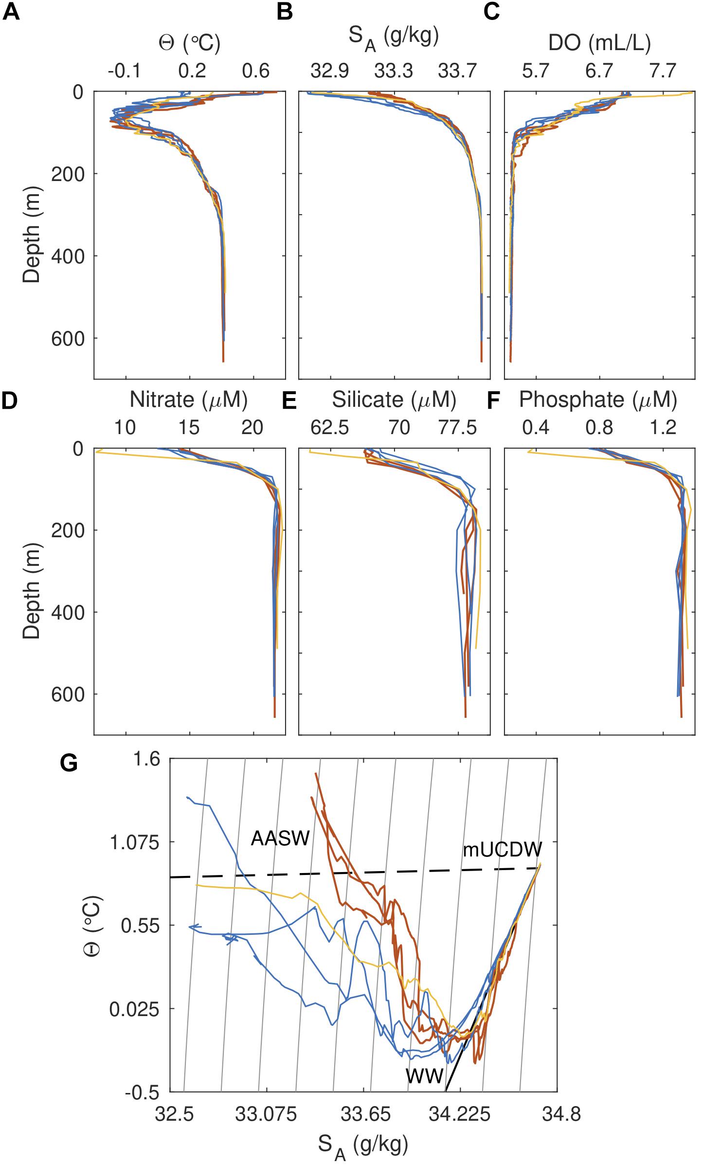
Figure 3. Profiles of (A) temperature, (B) salinity, (C) dissolved oxygen, (D) nitrate, (E) silicate, and (F) phosphate for occupied stations. Colors are as indicated in Figure 1C. (G) Temperature-salinity diagram for hydrographic stations. Gray lines indicate isopycnals, while the dashed and solid black lines correspond to the runoff and meltwater mixing line, respectively. Major water masses present in the region are indicated in black text. WW, Winter Water; mUCDW, modified Upper Circumpolar Deep Water; AASW, Antarctic Surface Water.
Physical differences in the properties of these water masses are paralleled by differences in their biogeochemical properties (Figures 3C–F and Supplementary Figure 3). Highest concentrations of nitrate (NO3 = 33.19 μM), phosphate (PO4 = 2.22 μM) and silicate (Si(OH)4 = 95.4 μM) are found at depth in mUCDW, with decreases noted within WW (mean NO3 = 31.40 μM, PO4 = 2.13 μM, Si(OH)4 = 86.70 μM) and AASW above [mean NO3 = 22.10 μM, PO4 = 1.48 μM, Si(OH)4 = 70.80 μM]. In contrast, dissolved oxygen concentrations are uniformly low in mUCDW below 120 m (mean DO = 5.01 mL/l) increasing toward a surface maximum in AASW (DO = 8.37 mL/l). Ammonium follows the same trend as oxygen, with maximum concentrations in surface waters (NH4 = 2.03 μM), becoming undetectable below 100 m (data not shown).
While a similar water mass structure is observed at stations within the bay, notable departures from properties outside of the fjord are also apparent (Figure 3 and Supplementary Figures 3, 4). Several warm water intrusions are present in the WW layer (max Θ = 0.10°C and max SA = 34.34 g/kg), with AASW waters above 40 m colder (min Θ = 0.48°C), fresher (min SA = 32.88 g/kg), and in some cases lighter than waters at our reference stations (min Θ = 1.16°C, min SA = 33.45 g/kg) (Figures 3A,B and Supplementary Figure 4). In Θ–SA space, this is reflected by a departure of fjord profiles from the ambient trend (i.e., lines in Θ–SA space linking mUCDW, WW, and AASW) observed on the shelf (Figure 3G). In examining fjord Θ–SA profiles in more detail, we notice that water-mass properties within the fjord fall between characteristic lines linking deep mUCDW to submarine melt and subglacial discharge endmembers, consistent with transformation of ambient waters through mixing with subglacial discharge and melting of the glacier termini.
Biogeochemical properties of bay water masses mirror these physical patterns of water mass transformation, with fjord waters between the surface and 150 m showing along-isopycnal enrichment of upward of 1–3 μM nitrate, 0.10–0.25 phosphate, and 3–8 μM silicate (Table 1, Figures 3D–F, and Supplementary Figures 3, 4), coupled with a dissolved oxygen deficit (0.1–1.12 mL/L) in WW and AASW relative to reference profiles on the shelf (Figure 3C and Supplementary Figures 3, 4). Mapping these anomalies as along-fjord sections shows that the coherent physical and biogeochemical property anomalies are strongest near the glacial terminus and weaken at the mouth, with the weakest anomalies found at the reference stations and at depth beneath the WW layer (Figure 4).
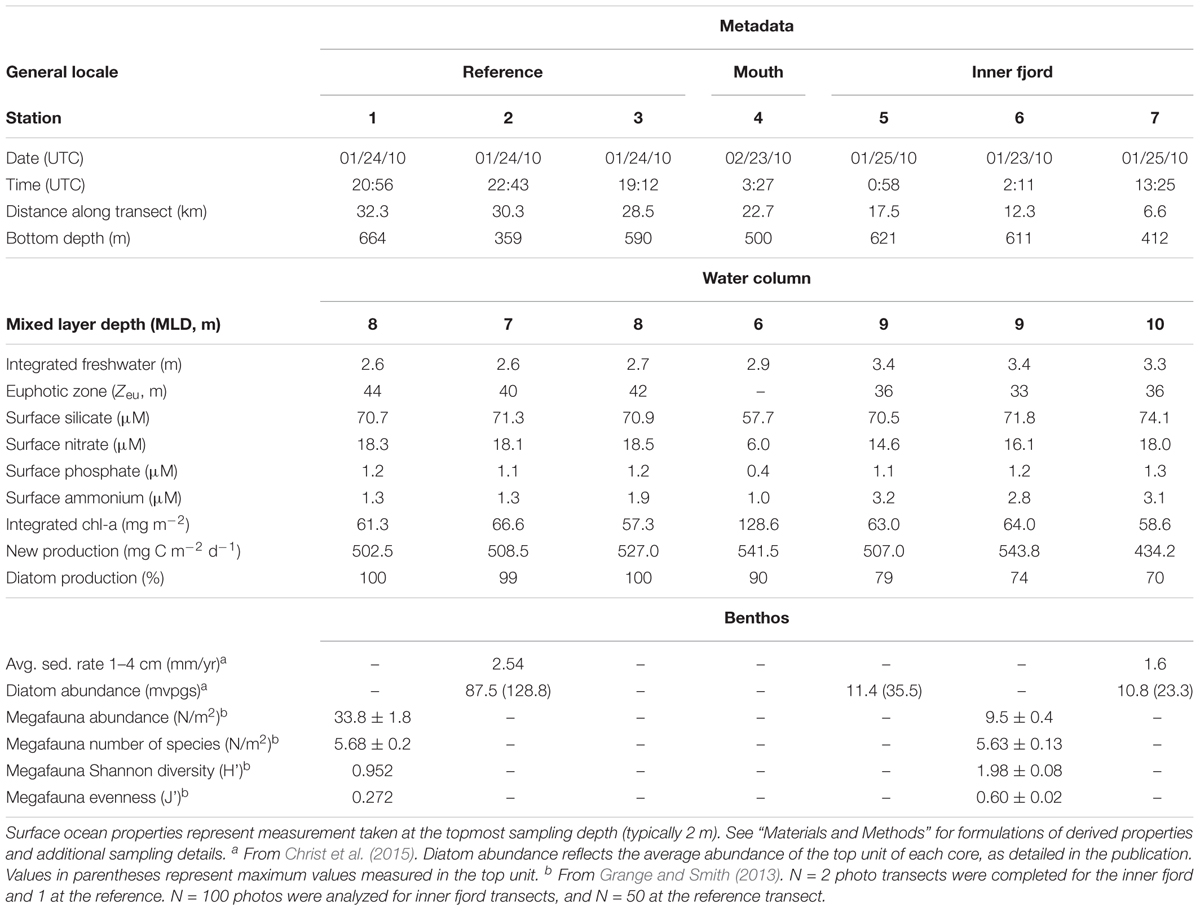
Table 1. Measured and derived properties of stations sampled in Barilari Bay during NBP1001.
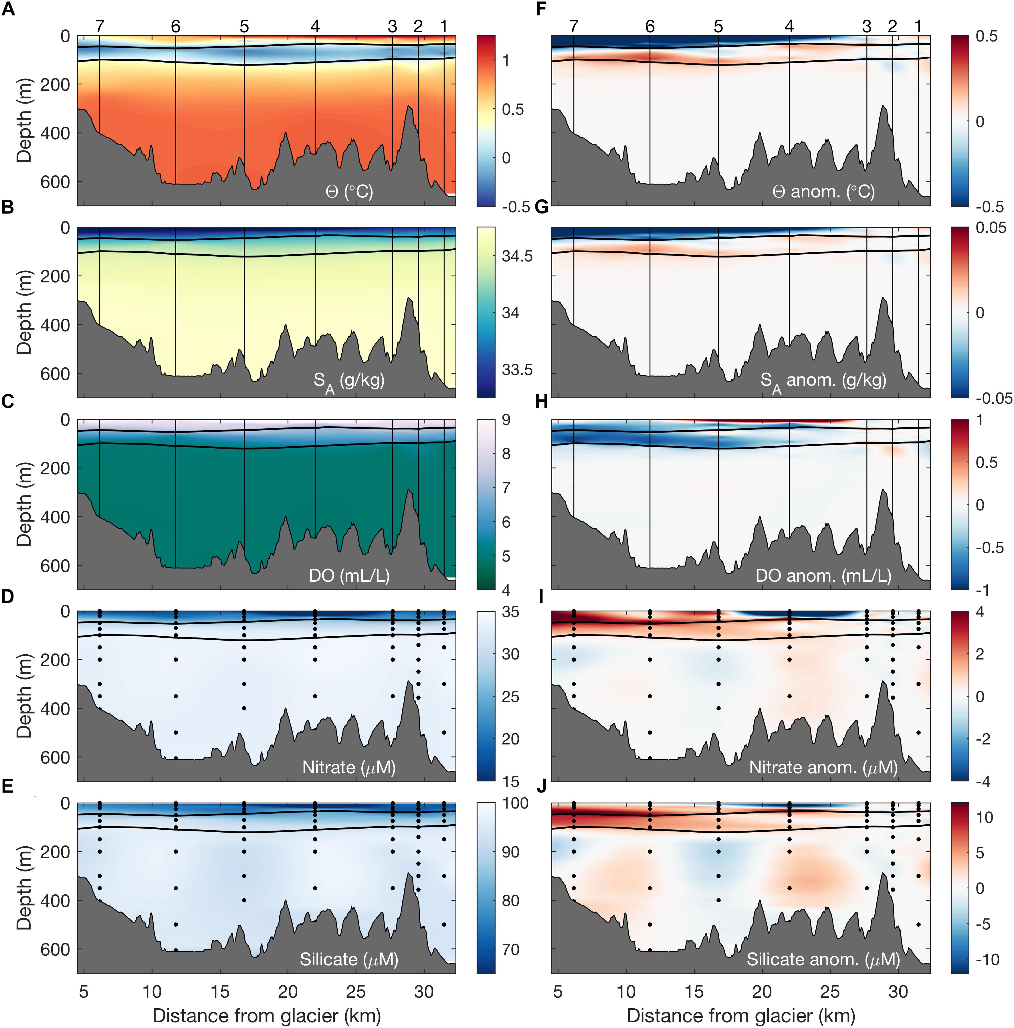
Figure 4. Along-fjord sections of (A) temperature, (B) salinity, (C) dissolved oxygen, (D) nitrate, and (E) silicate for the section shown in Figure 1C. Panels (F–J) show along-isopycnal anomalies calculated relative to a composite reference profile (i.e., an average of profiles at stations 1–3). Vertical lines and points indicate locations of continuous hydrographic profiles and discrete water sample collection, respectively. Black horizontal lines correspond to the σ𝜃 = 27.1 and 27.5 kg m-3 isopycnals, approximately delimiting the winter water layer in Barilari Bay.
In agreement with observed physical and biogeochemical gradients, examination of water column δ18O provides further evidence for glacial transformation within Barilari Bay (Figure 5). While highest δ18O are found in mUCDW (δ18O = -0.031 ± 0.086‰), gradual depletion in water column 18O is observed in WW and AASW above, with lightest values reaching δ18O = -0.61‰ at the reference stations (Figure 5A). We find consistently lower δ18O in upper bay waters (<75 m) compared to outside the fjord, with global minima of δ18O = -0.85‰ recorded at the surface of station 5 in January, and δ18O = -1.02‰ at station 4 in February, suggesting, alongside spatial gradients, temporal changes in water column meltwater inventories between the two occupations.
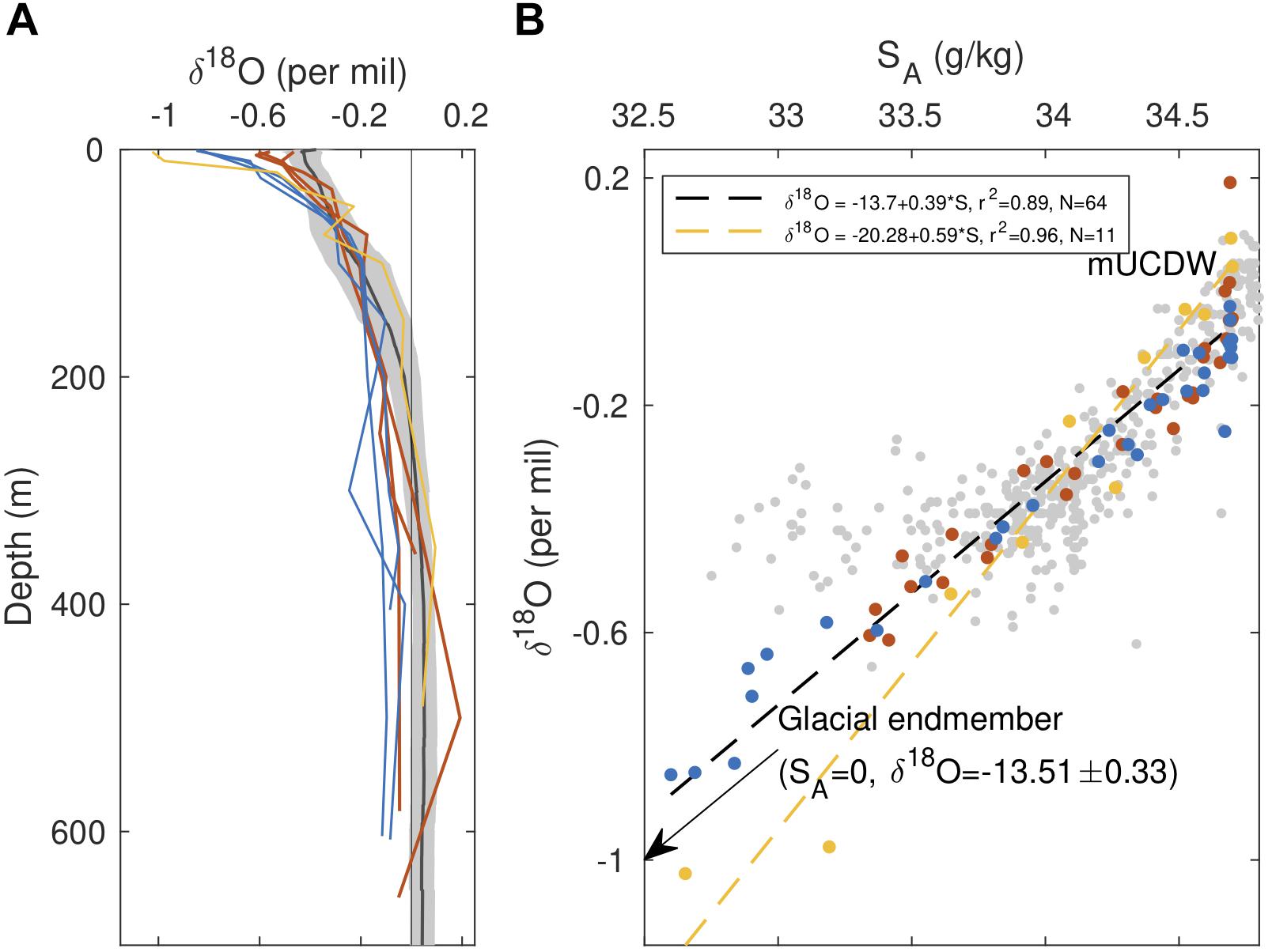
Figure 5. Pattern of glacial modification within Barilari Bay. (A) Profiles of δ18O, with colors as shown in Figure 1C. Black profiles indicate the mean δ18O profiles for continental shelf stations sampled between the 300 and 600 lines of Palmer-LTER (approximately 64–66°S), with properties averaged along isopycnals. Gray patch denotes one standard deviation about the mean. Gray vertical line denotes δ18O = 0‰. (B) δ18O-salinity plot for profiles shown in (A). Gray points are discrete measurements collected on the WAP shelf between the 300 and 600 lines of Palmer-LTER. Black and yellow dashed lines correspond to linear regressions on the full dataset from this study and station 4 (yellow points), respectively, with regression statistics shown in the legend.
In δ18O–SA space, properties of January stations are scattered along a line (δ18O = -13.70 + 0.3931SA, n = 64, r2 = 0.89) that nearly links the local mUCDW endmember and measured properties of glacial ice collected farther north in Brialmont Cove earlier in the cruise (SA = 0 g/kg, δ18O = -13.5 ± 0.33) (Figure 5B). While properties of station 4 waters appear to fall along a steeper line than those of January stations (δ18O = -20.28 + 0.59∗SA, n = 11, r2 = 0.96), these observations remain consistent with transformation of ambient water as a result of meteoric water injection, considering the large variability in the δ18O glacial endmember properties in the WAP reported in the literature (-20 < δ18O < -13; Meredith et al., 2008), as well as the observed variability in the deep-water properties (Figure 5A).
We put these oxygen isotope measurements in context by comparing them with properties of water masses sampled between the 400 and 600 lines of the Palmer LTER grid between 2011 and 2014 (Meredith et al., 2017), shown in Figure 5. Relative to the open WAP continental shelf, waters in the top 60 m of both reference and fjord stations are isotopically lighter, consistent with an expected pattern of increased glacial (meteoric) modification toward the coast (Meredith et al., 2013), with near-surface waters within the fjord lighter than all WAP shelf observations. Oxygen isotopes therefore suggest that waters at reference stations are glacially modified. While isotopic signatures of WW are similar across the shelf and Barilari stations, notable differences also emerge below 200 m, with January fjord stations and two reference stations showing lower δ18O values than those found along the WAP shelf. We also note that deep waters in the fjord, although seemingly unmodified in terms of their Θ–SA and other biogeochemical properties, also show a 1–4% lower beam transmission signal below 200 m, with a subsurface minimum of 89% recorded at inner fjord station 7 (Supplementary Figure 5). Water masses at station 4, while displaying the largest δ18O differences in surface waters relative to offshore, are also most similar to WAP profiles at depth.
Freshwater Budget
Hydrographic properties suggest that GMW is distributed in the top 150 m of the fjord. Our three models provide further insight into patterns of meltwater distribution within the fjord (Figure 6 and Supplementary Figures 6, 7). Concentrations of glacial meltwater, explicitly estimated in Mor13 and Jen99, increase starting at approximately 300 m depth, a depth coincident with the average estimated draft of the glaciers terminating in Barilari (247 ± 86 m; Figures 6B–H and Table 2). While concentrations below 150 m are relatively uniform across our sampling stations (<0.76%), greater separation between reference and fjord stations are present above, with a trend of increasing water column meltwater concentrations toward the inner fjord (maximum 1.38%) Increased scatter is observed within the euphotic zone (∼40 m), and particularly within the shallow surface mixed layer (∼9 m, Table 1), where the models yield either negative meltwater fractions (Mor13) or meltwater concentrations exceeding the theoretical maximum (Jen99) (Figures 6B–H and Supplementary Figure 6). Such departures indicate that processes other than submarine melt contribute to the observed patterns (e.g., atmosphere–ocean interactions), or potentially that water mass endmember are poorly specified (e.g., additional water masses are needed for the observed hydrography). Integrated below the mixed layer, water-column freshwater content derived from these estimates show a strong along-fjord gradient, with largest inventories observed near the glacial terminus (3.30–3.40 m) and lowest offshore (2.62 – 2.70 m; Table 1).
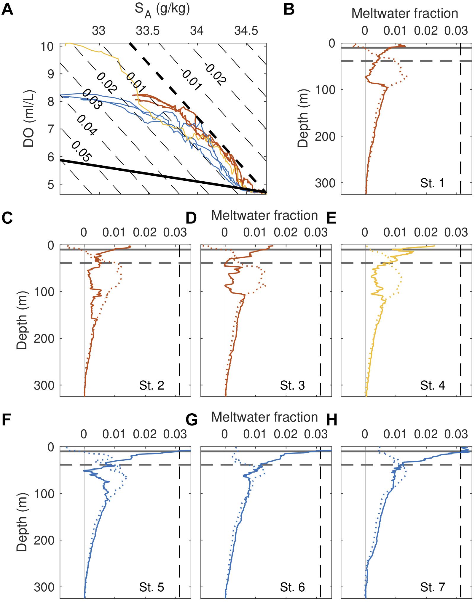
Figure 6. Water column glacial meltwater content and distribution. (A) Dissolved oxygen – salinity profiles. Dashed black line links properties of deep mUCDW and WW, and the solid black line links mUCDW and meltwater endmember properties. Gray contours correspond to isolines of meltwater fraction, computed following the Jen99 model. (B–H) Profiles of meltwater fraction for individual stations, with solid lines corresponding to estimates from Jen99 and dashed lines from Mor11. Dashed, black horizontal line corresponds to euphotic zone depth, while the solid black horizontal line indicates mixed layer depth. Dashed vertical line indicates the theoretical upper bound on meltwater fraction [Supplementary Equation (10)].
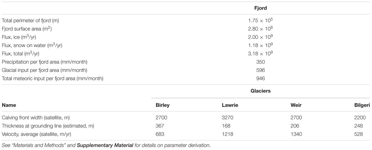
Table 2. Ice flux model parameters, including inputs and outputs.
Similarities are also observed in the meteoric water content of the water column, computed as the sum of subglacial and meltwater fractions (i.e., freshwater fraction) in Mor13 and resolved explicitly in Mer08. Meteoric water fractions show an almost monotonic vertical increase (Supplementary Figure 7), with a maximum value of 7.3% found at the surface of station 4. Fractional sea ice melt contributions, computed in Mer08, are by comparison small (<0.05%) and often negative (not shown). An along fjord-gradient mimicking meltwater is also present, with highest water column meteoric water concentrations found near the glacier and lowest at the reference stations. The two models also show a high degree of fidelity, with magnitudes and trends similar for both estimates.
Ocean Circulation
Property profiles (Figures 3, 5), along-fjord anomalies (Figure 4), and derived meltwater concentrations (Figure 6) indicate that meltwater primarily transits out of the fjord in an approximately 150 m-thick near surface plume. For a simple estuarine circulation, this flow should be balanced by an inflow of unmodified waters at depth, an expectation supported by the weaker physical and biogeochemical anomalies observed in this layer (Figure 4).
Hydrographic datasets delimit an upper and lower layer in the fjord coinciding with the extent of the observed property anomalies. ADCP observations demonstrate a complex flow patterns within these two layers. In January, we observe weak inflows <7 cm s-1 within the top 150 m, spatially accentuated along the NE side of the bay (Figure 7A). Ocean currents reach a maximum speed of 12.52 cm s-1 at station 1 in the middle bay. Outflows in the same layer are only found along the southwest portion of the bay, with along-fjord velocities reaching 8 cm s-1, resulting in a gyre-like circulation inside Barilari Bay in that layer. Significant cross-fjord flow is also noted, with cross-fjord velocities overall stronger (>6 cm s-1) than along-fjord velocities (<6 cm s-1), highlighting the influence of rotation on circulation. Below 150 m, velocities are generally weaker than near the surface, except near the glaciers at station 1, where we observe maximum velocities of 6.55 cm s-1 at 256 m (Figure 7B). We also find a secondary, eddy-like circulation at the fjord mouth near our three reference stations. In February, we find instead weak outflow in waters <150 m along our cruise track, apart in the middle bay near station 1 where we note inflows upward of 8 cm s-1 (Supplementary Figure 8). Deep currents <150 m are in turn dominated by weak inflows (<2 cm s-1), with maximum velocities found near station 1.
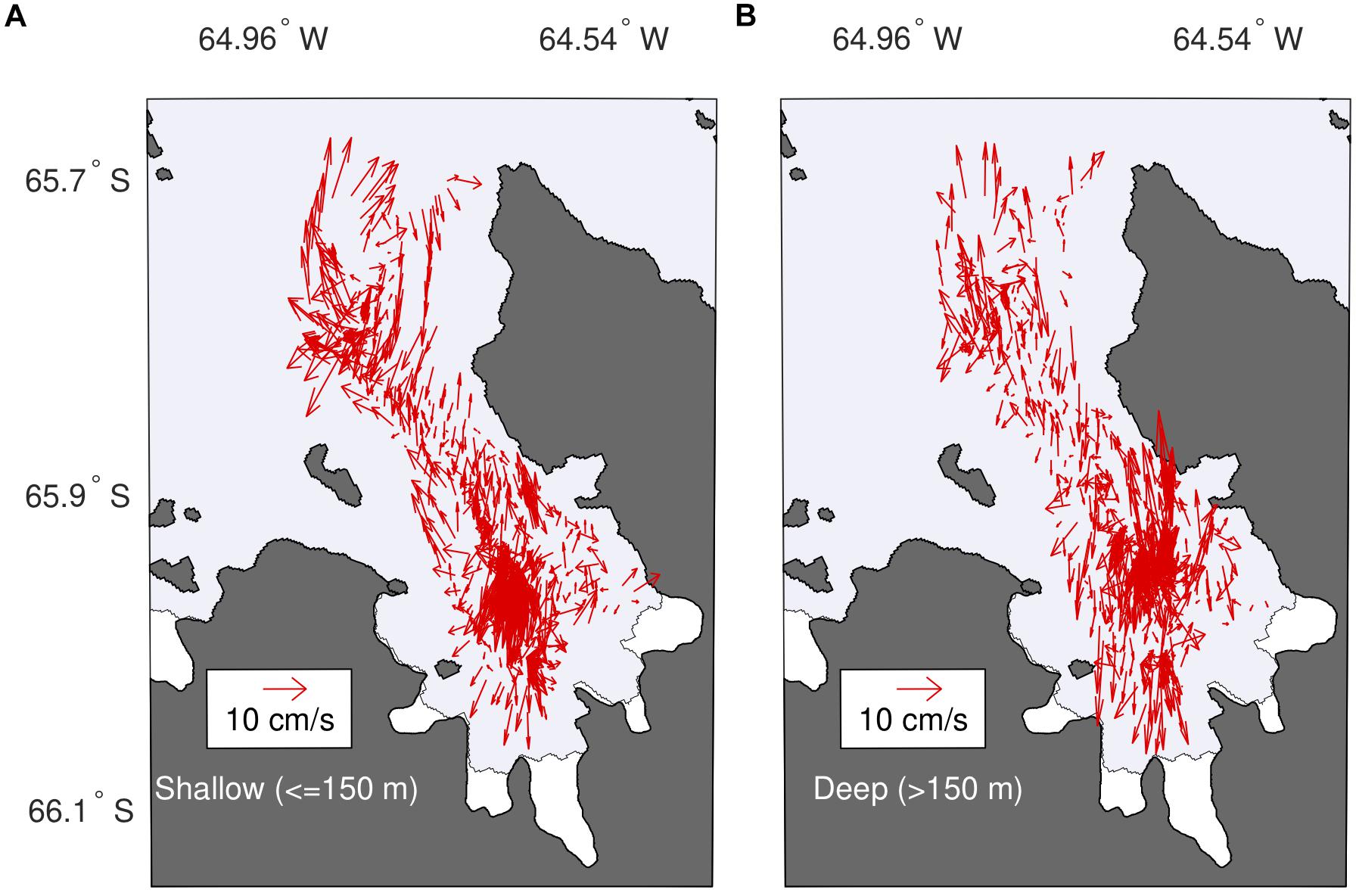
Figure 7. Shipboard ADCP-derived circulation within the bay. Vertically averaged current velocity for the (A) upper 150 m of the water column, and (B) for waters below 150 m. Layer depths were chosen to reflect anomaly patterns shown in Figure 3.
Examination of lowered ADCP data corroborate these observations (Supplementary Figure 9). While the strongest velocities are found in the top 150 m of the water column, they indicate an inflow of water at all but one fjord station at the time of sampling and at two reference stations, with indication of outflow in this upper layer found only at innermost station 7. Beneath this more energetic upper layer, flows are weak (<3 cm s-1) and reversing at all but station 7, where stronger (>5 cm s-1) cross-fjord currents across the fjord are present between 200 and 300 m.
Glacial Fluxes and Surface Mass Balance
Surface mass balance data derived from RACMO2 and ice balance fluxes provide insight into the sources of freshwater delivered to Barilari. As a result of the steep topography of the Antarctic Peninsula and the prevalent synoptic westerly flow, net input of freshwater as precipitation over the fjord area is high, averaging 350 mm/month (4.20 m/year) (Table 2). This estimate is in agreement with previous surface mass balance results for WAP near-shore regions (>300 mm/month; Meredith et al., 2013), and is far larger than averages for the WAP shelf as a whole (∼50 mm/month). In turn, average ice fluxes into the bay from our four primary glaciers (Birley, Lawrie, Weir and Bilgeri; i.e., omitting any glacial flow outside of these glacial streams), equate to an additional freshwater input of 596 mm/month, or 7.15 m/yr. This yields a total freshwater input of 946 mm/month, averaged over the fjord area, compared to an area-averaged 130 mm/month for the WAP shelf (Meredith et al., 2013).
Consideration of freshwater volume derived from δ18O in concert with these fluxes provide an estimate of the residence time of water in the ford. With an average freshwater volume of 3.25 ± 0.21 m for inner fjord stations, and an estimated annual combined freshwater input of 11.36 m/yr, residence time for freshwater in this system is approximately 3.4 months.
Ecosystem Response
Phytoplankton Biomass and Community Composition
Phytoplankton biomass exhibits significant changes between our two occupations of the bay (Table 1 and Figure 8). In January, maximum in vivo chl-a concentrations at inner-bay stations are relatively uniform, ranging from 1.81 to 1.88 mg m-3, with a local chl-a maximum found on the shelf at reference station 3 (chl-a = 2.32 mg m-3). Chl-a maxima are found at 10 m depth within the bay and at the surface (2–5 m) at shelf stations. By comparison, vertically integrated biomass shows a positive trend within the bay, with lowest biomass at the inner fjord (chl-a = 58.6 mg m-2) increasing away from the glacier (63–64 mg m-2), with offshore values more variable yet on par with fjord biomass (57.3–66.6 mg m-2). Along-track extracted and in vivo chl-a fluorescence, measured from the seawater intake, show a similar pattern with a gradual increase in chl-a biomass toward the mouth of the fjord (Figure 8C).
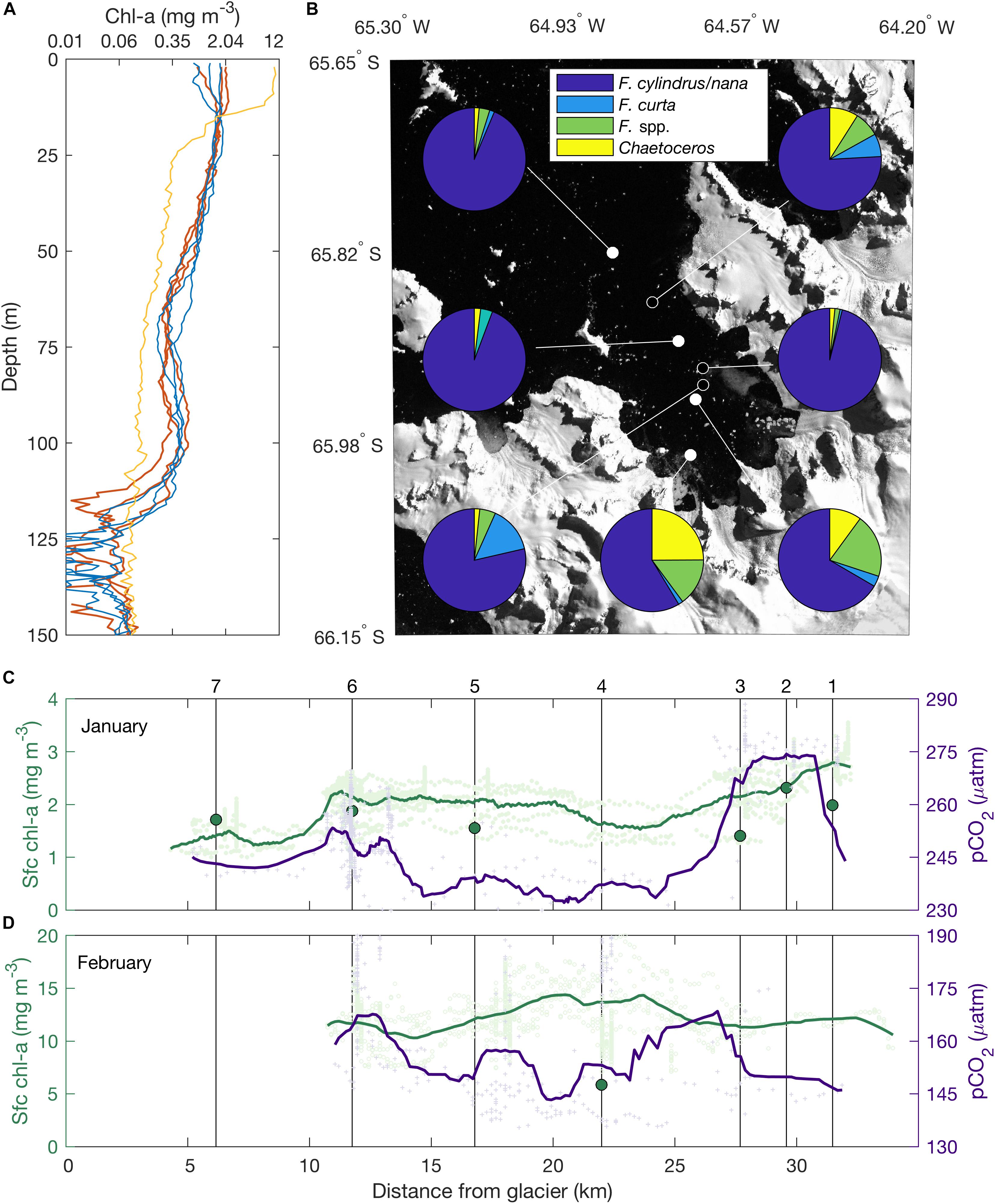
Figure 8. Phytoplankton biomass, community composition, and CO2 drawdown. (A) Vertical profiles of in vivo chl-a biomass. Note the log scale. (B) Diatom community composition of surface waters sampled from the ship’s flow-through system. Stations sampled in January and February are indicated by filled and hollow white points, respectively. Along-track, surface chl-a and pCO2 measured in (C) January and (D) February along the section shown in Figure 1A. Note changes in scales. Dark green points indicate discrete extracted chl-a samples collected from the ship’s flow through. Light green and purple points correspond to discrete measurements of in vivo chl-a and pCO2, respectively, with low-pass filtered data indicated by colored lines. Station locations are noted by black vertical line.
In February, chl-a biomass measured at station 4 is threefold higher than in January, with maximum in vivo chl-a exceeding 12 mg m-3 (Figure 8A), extracted chl-a concentration in the 1 μm size fraction reaching 5.86 mg m-3 at the surface, and integrated chl-a reaching 128.6 mg m-2, twofold higher than in January. While we lack complementary hydrographic stations from the inner fjord in February, along-track in vivo fluorescence indicates a similar spatial pattern to January, with a gradual increase in chl-a concentration between the inner bay and the mouth and decreases beyond (Figure 8D).
Fragilariopsis cylindrus/nana dominates the diatom community across our sampling region (>56.1%) (Figure 8B). The rest of the assemblage is composed of other species of Fragilariopsis, generally sea-ice associated species such as F. curta, with many of the specimens of Fragilariopsis spp. occurring in girdle view, usually in colonies, and consequently difficult to identify to species level. There is a spatial and temporal shift in community composition between January and February. First, diatom abundance increases by 1–2 order of magnitudes between January (0.27 ± 0.08 million valves) and February (10.81 ± 6.61 million valves). In January, inner and mid-bay samples show a higher frequency of F. spp. and Chaetoceros subg. Hyalochaete (Fragilariopsis spp.:14.3–19.1%; Chaetoceros spp.: 9.6–23.82%) than at the mouth or on the shelf (Fragilariopsis spp.: 3.1–3.6%; Chaetoceros spp.: 1.4–1.9%), with corresponding changes in the frequency of F. cylindrus/nana (56.1–63.6% inner bay, 87–90.7% mouth and shelf). In February, F. cylindrus/nana frequency increases in the inner-bay stations relative to January (78.6–95.6%). The highest abundance of diatoms is found within the bay (17.64 million valves). High abundances are, however, also found beyond the fjord mouth, with F. cylindrus dominating the assemblage (>99%), and diatom concentrations ranging from 10.1 to 15.6 million cells l-1. Other notable changes include an increase in the frequency of Chaetoceros subg. Hyalochaete at the mouth (8.5% of the assemblage) and decreases in the bay (1.6–1.7%), as well as an increase in the frequency of F. curta in both locations (0.7–14.7%).
CO2 Drawdown and Productivity
Gradients in surface pCO2 are also apparent in our study area. January pCO2 concentration range from a minimum of 234 μatm at the mouth of the fjord to a maximum of 274 μatm at the reference stations, with higher values also noted in the inner fjord than at the mouth (Figure 8C and Supplementary Figure 10). High pCO2 at the reference stations coincides with relatively higher chl-a concentrations, surface temperatures, and surface salinities compared to within the fjord (Supplementary Figure 10), indicative of the combined impact of physical, chemical, and biological processes on surface pCO2. While a gradient is also present in February, pCO2 values are significantly lower at that time, with observations throughout the study area not exceeding 172 μatm (Figure 8D and Supplementary Figure 10).
Surface waters are undersaturated in CO2 with respect to the atmosphere across all our occupations (Supplementary Figure 10), with atmospheric concentrations ranging from 371 ± 1.90 μatm in January to 378.50 ± 1.42 μatm in February. Mean daily CO2 air to sea exchange for the fjord, estimated for the period spanning January 22 to February 22, ranges between -0.76 ± 1.05 and -1.69 ± 1.24 g C m-2 d-1 depending on the form of the gas exchange parametrization (Supplementary Figure 11). Both average and standard deviations are large, owing to the large ΔpCO2 between atmosphere and ocean and the occurrence of multiple strong wind episodes within the bay, with AMPS-derived average daily wind speeds exceeding 10 m s-1 for 15 out of 31 days during this period (Supplementary Figure 12). Median values are by comparison significantly lower (-0.28 to -0.47 g C m-2 d-1; Supplementary Figure 11), owing to the strongly skewed nature of the daily air to sea fluxes. Considering 10-day averaged wind speed as opposed to daily means leads to mean fluxes ranging between -0.55 ± 0.36 and -0.91 ± 0.58 g C m-2 d-1 and a doubling of median estimates (-0.56 to -0.93 g C m-2 d-1; not shown).
We compare these carbon drawdown estimates to phytoplankton primary production in the bay derived from vertical gradients in nutrient concentrations (Hoppema et al., 2002) (Table 1). Based on patterns of nutrient drawdown, which we assume represents an integral of nutrient uptake between October 1 and our occupation of Barilari, inner fjord stations sampled in January support an average new productivity (e.g., based on nitrate uptake) of 434 mg C m-2 d-1. Productivity increases to 507–544 mg C m-2 d-1 toward the fjord mouth and generally decreases beyond (502–527 mg C m-2 d-1). Considering differences in nutrient inventories at the mouth of the bay (assuming similarity in water mass properties at stations 4 and 5) only between our January and February occupations yields a mean productivity of 604 mg C m-2 d-1 over that time period. Most of this productivity is due to diatom growth, as indicated by the significant silicic acid drawdown and our analysis of community composition (Figure 8B and Table 1). However, notable differences are also present between reference and fjord stations, with diatom contributions at reference stations (>99%) much higher than those at inner fjord stations (74–79%).
Bentho-Pelagic Coupling
Synoptic gradients in water column physical and biological properties are paralleled by gradients in the benthos (Table 1). Sedimentation rates at station 7 are lower (1.6 mm/yr) than at the reference stations (2.54 mm/yr), with a concurrent monotonic increase in sediment diatom abundance between the innermost station (average 10.8 million valves per gram sediments – mvpgs) and the reference station (87.5 mvpgs).
Lower megafauna abundance is also observed proximal to the glacier (9.5 ind m-2), increasing toward to the fjord mouth (33.8 ind m-2) (Table 1). Nevertheless, these values are significantly higher than those observed on the open WAP shelf (Smith et al., 2006; Grange and Smith, 2013). Patterns of megafaunal diversity are more complex. While the total number of species per sample (richness) found at the inner fjord and reference stations is similar (5.63 ± 0.13 and 5.68 ± 0.2, respectively), evenness (a measure of species distribution among individuals) is higher in the inner fjord (J’ = 0.596 ± 0.016) compared to the reference stations (J’ = 0.272).
Discussion
In sampling a near-shore system along the WAP, this study provides important observational data to constrain ocean properties at the glacial margin and elucidate the impact of ice–ocean exchange on coastal biogeochemistry and carbon cycling. Our survey of Barilari Bay indicates that warm mUCDW, presumed to be the source of heat contributing to submarine melt along the AP (Wouters et al., 2015; Cook et al., 2016), is present throughout the bay and reaches the glacial terminus, as suggested by our innermost profile collected 7 km from the glacial terminus (Figures 3, 4). Integrated physical and biogeochemical observations further demonstrate that ocean waters entering Barilari Bay undergo significant modification (Figures 3–5 and Supplementary Figures 3–5) which is consistent with interaction with the ice sheet and, in particular, the injection of glacial meltwater into the water column at depths of up to 300 m (Figures 3–6 and Supplementary Figures 3–5). The result is the production of a 150 m thick layer of glacially modified water, whose properties are set by the interaction of ambient water masses and the ice sheet. We show that these interactions contribute to the enhancement of near-surface (<150 m) nutrients (Figures 3, 4, Supplementary Figures 3, 4, and Table 1), with ramifications for phytoplankton at the base of the food web and patterns of organic matter export. While this survey therefore presents a coherent, integrated picture of the connection between ice–ocean interactions and the WAP marine ecosystem, it also raises several intriguing uncertainties and potential future research pathways in this important region.
Circumpolar Deep Water Distribution and Modification
The consistent physical (e.g., Θ–SA) and biogeochemical (e.g., nutrients, δ18O) property anomalies observed in the fjord (Figure 4), and in particular, the high temperature, low oxygen intrusions within WW (Figure 3 and Supplementary Figures 3, 4), alongside the depletion of oxygen in AASW relative to the continental shelf, suggest that warm, oxygen-poor mUCDW contributes to the glacially modified mixture (Jenkins, 1999; Dutrieux et al., 2014), and indeed interacts with the glacial front. In this framework, mUCDW advected toward the glacial margins contributes to submarine melting, which along with any input of subglacial discharge (runoff), leads to the formation of a buoyant plumes that rise, entraining mUCDW and redistributing both glacial meltwater and ambient waters vertically (Figure 3). This is a significant finding, given that these are among the first observations showing that mUCDW reaches the glaciers along the WAP continental margin and contributes to submarine melting.
Given that mUCDW can access the glacial terminus in Barilari Bay, our observations suggest that warming and shoaling of mUCDW, as already observed on the WAP continental shelf (Martinson et al., 2008; Schmidtko et al., 2014; Spence et al., 2017), may have important consequences for melt rates of tidewater glaciers and glacial dynamics in this region. However, Θ–SA properties also indicate that mUCDW found in Barilari Bay cools significantly during its transit to the glacial margin. Hydrographic data collected approximately 10 days prior to our occupation of Barilari during January 2010 (by the Palmer LTER cruise aboard the R/V Laurence M. Gould, not shown) shows a subsurface temperature maximum of Θ = 1.86°C between 375 and 400 m depth at the shelf break along the 500 line (Figure 1A), with temperatures decreasing to Θ = 1.61°C at 340 m mid-shelf offshore of Renaud Island and finally to Θ = 0.93°C within the bay. While previous studies demonstrated such a cooling trend across the open WAP shelf (Martinson et al., 2008), we show here that it extends to the glacial margin. Similar temperature decreases have been observed elsewhere along the WAIS margins, including in Pine Island Bay (Jacobs et al., 2011; Dutrieux et al., 2014). While strengthening of circumpolar winds may therefore advect greater volumes of mUCDW onto the shelf as a result of eddy activity (Martinson et al., 2008; Martinson and McKee, 2012), this may not necessarily result in warmer waters reaching the glacial margins. More extensive observations in bays and fjords such as Barilari Bay are needed to constrain the properties and sources of variability of waters interacting with the ice sheet, and whether these, like mUCDW on the shelf, are undergoing any long-term changes.
Glacial Inputs, Distributions, and Concentrations
Glacially modified waters form as a result of mixing between ambient waters, subglacial discharge, and submarine meltwater are identifiable as along-fjord along-isopycnal anomalies (Figure 4 and Supplementary Figure 4). These waters are distributed in the top 150 m of the fjord, with highest concentration of glacially derived freshwater found at the surface, as evidenced by the minima in δ18O (Figure 5). The δ18O signal in Barilari Bay, while lighter than previously quantified offshore (Figure 5), is nevertheless consistent with the distributions observed on the continental shelf as well as the trend of increased meteoric water content toward the coast (Meredith et al., 2013, 2017). This trend is a result of the proximity of coastal glacial inputs and the impact of the AP orography on precipitation. These patterns underline two important points regarding meltwater distributions along the WAP shelf: (1) processes occurring along the AP glacial margins shape the distribution of meteoric water. Shelf processes (e.g., wind-driven mixing, sub-mesoscale dynamics) then modulate this distribution in space and time as fjord waters are exported to WAP shelf. And (2) as a result of injection at depth of subglacial discharge and submarine meltwater in a stratified water column, a portion of the glacially modified water plume can reach neutral buoyancy subsurface, as observed here within the WW (Figures 3, 4 and Supplementary Figures 3, 4). In particular, a subsurface plume expression is expected when weak buoyancy forcing is present (Sciascia et al., 2013; Carroll et al., 2015), as previously observed at the margins of icebergs (Stephenson et al., 2011), and as is likely the case in Barilari Bay given the purportedly weak subglacial (runoff) forcing at the glacial margins and low melt rates (Pettit et al., 2015b). We expect such broad meltwater distributions to be a feature of most glacial fjord systems along the Antarctic Peninsula, given similarities in their oceanographic and glaciological setting (see Powell and Domack, 2002, for similar conclusions).
Comparing hydrographic profiles to model-derived estimates of meteoric water content underscores additional feature in the properties and distribution of glacial meltwater. Despite differences in the derived vertical gradients and magnitude (Figure 6 and Supplementary Figures 6, 7), a trend of increasing vertically integrated meltwater content toward the inner fjord is apparent in Jen99 and Mor13, mirroring increases in the magnitude of along-isopycnal property anomalies. Furthermore, these models also indicate that meteoric water (or in the case of Mor13, the combination of submarine meltwater and subglacial discharge) comprise a maximum of 7% of glacially modified water volume (Supplementary Figure 7). In other words, GMW is primarily composed of ambient water masses (>93% in Mer08 and Mor13), a common feature observed in glacially influenced systems globally (e.g., Jenkins and Jacobs, 2008; Beaird et al., 2015; Cape et al., 2019), which underscores the ocean’s critical role in mediating ice–ocean interactions and properties of the resultant ambient-glacial mixture.
Divergences between model estimates illustrate inherent uncertainties in the quantitative derivation of GMW water mass composition. Assuming a single water mass interacting with the glacier, Mor13 predicts a gradual vertical increase in meltwater concentration, reaching a global maximum in the WW layer (0.9–1.38%). On the other hand, Jen99, considering properties of an ambient water column composed of two primary water masses (mUCDW, WW), instead shows a local minimum meltwater concentration in that layer (Figure 6), a feature most accentuated at the reference stations. In some cases, the assumption of a single water mass interacting with the ice sheet is appropriate, as demonstrated in a previous analysis of meltwater distributions at the margins of George V ice shelf (Jenkins and Jacobs, 2008). In our case, properties of the ambient water column (e.g., linking mUCDW to WW) overlap with the melt line in Θ–SA and δ18O–SA space (e.g., Figures 3G, 5B); Θ–SA and δ18O–SA are variables that are used to define endmember properties in Mer08 and Mor13. Because they neglect the complexity of the local hydrography, and although Mer08 includes sea ice as a third water mass endmember, these models ultimately assign water column freshening with respect to mUCDW to the injection of meteoric water (with minor contributions from sea ice melt in Mer08). In our case, this overlap between properties of ambient and potentially glacially influenced waters ultimately hinders any objective parsing of ocean and glacial contributions. Additional independent tracers of water mass interaction, such as noble gases (Loose and Jenkins, 2014), are needed to account for the number of water masses present in Barilari and similar systems and can reduce uncertainty in derived fractions.
The mode of export of glacial meltwater to the marine environment (e.g., whether liquid export at the glacier bed or from melt at the glacial terminus) determines its impact on the physical and chemical marine environment (Straneo and Cenedese, 2015). A relatively warm climate will enhance surface melting of the glaciers, potentially increasing the supply of meltwater to the bed and contributing to a larger subglacial outflow. Relatively high snowfall, on the other hand, will reduce both surface and internal melting of the ice sheet, decreasing the supply of meltwater to the bed (Pettit et al., 2015b). In this region of sub-freezing temperatures (Supplementary Figure 1), melt rates of less than 0.1 m equivalent water per year (10 cm; RACMO2), and ice thicknesses >300 m suggest little, if any, surface melt can infiltrate the glaciers without refreezing. In other words, these conditions should favor reduced meltwater to the bed and low sub-glacial meltwater flux into the ocean. However, considering that the saturation submarine meltwater concentration (i.e., resulting from ocean water melting the ice) at the surface freezing point is approximately 3% for the observed hydrography (Jenkins, 1999), the subglacial fractions computed from Mor13 (>6%), as well as the high meteoric water content in Mer08, point to additional sources of meteoric water to the marine environment (i.e., subglacial discharge, surface runoff, precipitation; Supplementary Figure 7). Independent, qualitative evidence for a subglacial meltwater contribution is present in the form of lower beam transmission in the lower water column (Supplementary Figure 5), which is consistent with the export of particulates contained in subglacial discharge from the glacial bed. The magnitude of this subglacial flux remains uncertain. Derived subglacial discharge fractions from Mor13 are larger than expected, with magnitudes on par with those observed in Greenland glacial systems where subglacial discharge fluxes are significant (Chu, 2014). Precipitation, contributing on average 0.35 m of freshwater per month to the surface ocean (Table 2), could account for a portion of this non-meltwater source, with the remainder sourced from surface runoff. Convective or wind-driven mixing within the fjord would nevertheless have to accompany these surface fluxes to yield the observed meltwater distributions. A more nuanced understanding of the partitioning of glacial freshwater input along the coastal AP is needed to better constrain ice–ocean exchanges in this and similar systems.
Coastal Circulation
In Greenland and Alaskan glacial fjords, ice–ocean interactions, and specifically the export of subglacial discharge, acts as an important driver for circulation during the summer (Jackson and Straneo, 2016; Jackson et al., 2017), contributing to a buoyancy-driven estuarine outflow in an upper layer with velocities often reaching tens of centimeters per second. Barilari is by comparison a quiescent system, with flow speeds remaining below 7 cm s-1 (Figure 7 and Supplementary Figures 8, 9), i.e., of the same order as tidal velocities in this region (not shown). An average inflow or outflow is furthermore hard to discern in the ADCP datasets, owing to the low velocities as well as our short sampling timescale, with rotational dynamics evident in both upper and lower layers. These observed flow patterns are consistent with idealized fjord models forced by low subglacial discharge (Carroll et al., 2015; Sciascia et al., 2013), suggesting that in this system, export of meltwater from the glacier terminus contributes only weakly to fjord-scale circulation.
Shelf density fluctuations, along-fjord winds, and tides can act as additional drivers of fjord flows and fjord-shelf exchanges (Farmer and Freeland, 1983; Cottier et al., 2010; Stigebrandt, 2012; Spall et al., 2017). The extent to which these processes dominate in Barilari Bay is beyond the scope of this paper. However, it is informative to consider how these might impact fjord processes as they relate to meltwater export and biogeochemical cycling. While the oscillatory nature of tides contributes to mixing of fjord and shelf waters and the homogenization of observed properties (Farmer and Freeland, 1983), shelf and along-fjord winds can also drive pronounced, pulsed exchanges between fjord and shelf. For a deep, stratified fjord, the magnitude of this exchange for strong (>16 m s-1) wind events can be large, ranging between 10–50% of the upper layer and 7–15% of the lower layer for a single event (Jackson et al., 2014; Spall et al., 2017). In Barilari, such exchanges draw in shelf-derived mUCDW below, contributing to increased melt rates and leading to the export of surface GMW. Fjord profiles provide modest evidence for this mechanism. The period between our occupations of Barilari was marked by several strong, upwelling favorable wind events (Supplementary Figure 12), which could drive shelf density fluctuations and contribute to inflow of mUCDW at depth. Fjord properties at station 4 are consistent with these expectations (Figure 3 and Supplementary Figures 3, 4), with deep waters >150 m appearing more reference-like (warmer) than fjord stations sampled in January (Figure 3 and Supplementary Figure 4), and waters above showing evidence for enhanced meteoric water input and productivity during this time-span (Figures 5, 8C).
Despite playing only a weak role in driving fjord circulation at present, ice–ocean exchanges, and thereby circulation at the glacier termini, may become enhanced in the future if the warming trend along the Antarctic Peninsula continues. Barilari Bay lies near the northern limit of the mUCDW distribution, with deep waters north of Anvers Island instead influenced by colder, deep Weddell Sea Deep Water (Figure 1A). Enhanced surface melt of the ice sheet due to atmospheric warming could in the future contribute to greater runoff into the fjord, with injection of larger volumes of meltwater at up to 300 m depth invigorating the marine circulation, contributing to greater heat fluxes to the glacial margins. Given the dynamic coupling between subglacial discharge and upwelling rates of ambient waters (Jackson et al., 2017), these physical changes would in turn have important consequences for WAP marine ecosystems.
Vertical Nutrient Fluxes and Fjord-Shelf Exchanges
Marine terminating glaciers and ice shelves fundamentally shape the biogeochemical properties of coastal waters (Hartley and Dunbar, 1938; Dunbar, 1973; Jacobs et al., 1979; Horne, 1985; Gerringa et al., 2012; Meire et al., 2017). Export of meltwater at the glacial margins contributes to the stratification of the water column while bringing to the euphotic zone essential nutrients for the growth of phytoplankton (Figures 3, 4 and Supplementary Figure 4). These processes can in turn serve to support high rates of secondary productivity, for which there is growing evidence for AP glacial systems (Nowacek et al., 2011; Grange and Smith, 2013). While this process has previously been detailed along other Antarctic glacial margins including Pine Island Bay and McMurdo Sound (Jacobs et al., 1979; Gerringa et al., 2012), our observations are one of the first to provide in situ evidence for this enhancement along the Antarctic Peninsula. The magnitude of the enrichment may seem modest relative to the fjord nutrient standings stocks (Figures 3, 4 and Supplementary Figures 3, 4), particularly considering recent observation from Greenland glacial fjords (Meire et al., 2017; Kanna et al., 2018; Cape et al., 2019). Yet, the observed patterns underscore several important facets of nutrient fluxes along glacial margins.
First, macro-nutrient enrichment is evident throughout the length of the fjord, peaking at the inner fjord stations and decaying away toward the reference stations (Figure 4). This demonstrates that ice–ocean interactions impact nutrient availability throughout this system, a fact that likely holds for other AP glacial fjords. While the trend in nutrient enrichment is robust, we argue that its magnitude conservative, considering the glacially modified nature of waters at our nominal reference stations (see Glacial inputs above; Figure 5). As a point of comparison, WW nitrate and silicate inventories 100 km away from the entrance to Barilari, measured at the same latitude along the 500 line during the January 2010 LTER cruise, are 2–4 μM lower than those observed at our reference stations (not shown). Greater understanding of circulation pathways between the open shelf and nearshore regions would enable better identification of source waters to Barilari and derivation of a more robust estimate of nutrient enrichment.
Second, given that a large volume of GMW is found below the euphotic zone (Figure 4 and Table 1), our observations suggest that a significant fraction of nutrient-enriched waters could be exported to the continental shelf unmodified, where they could contribute to biogeochemical cycling as previously hypothesized (Dierssen et al., 2002; Vernet et al., 2008; Meredith et al., 2013). Spatial and temporal changes in phytoplankton biomass during our survey support these assertions. Standing stocks of nutrients in January were high in surface waters (nitrate: 18.7 μM, phosphate: 1.21 μM, silicate 70.9 μM, ammonium: 1.87 μM), with comparatively modest phytoplankton biomass (max chl-a = 1.21 mg m-3) (Table 1 and Figures 3, 8). In late February, near end of the austral summer growth season, we instead observed significant nutrient drawdown (nitrate: 6.0 μM, phosphate: 0.4 μM, silicate 57.70 μM, ammonium: 1.04 μM; Table 1) coupled with a diatom bloom and significant pCO2 undersaturation of surface waters (Figure 8). Despite this biologically driven nutrient drawdown, evidence for nutrient enrichment in deep waters (40–150 m) of station 4 is nevertheless present, suggesting that glacial modification may contribute to regional productivity on the continental shelf in addition to carbon cycling within the fjords.
Third, the observed macro-nutrient enrichment represents the integrated result of the combined injection of meltwater into the water column and the resulting buoyancy-driven redistribution of glacial and ambient waters. In other words, nutrient inventories in glacially modified waters reflect not only the relative proportions of glacial and ambient water masses present in the mixture, but also the nutrient properties of these endmembers. While water mass analysis in this and other systems demonstrate that ambient waters form the dominant component of glacially modified waters (>90%), constraining source water properties for tidewater systems is difficult, particularly for glacial endmembers. Nutrient concentrations in glacial ice span 1–2 orders of magnitude with significant spatial heterogeneity (Wadham et al., 2013; Hawkings et al., 2015). While we lack local meltwater or glacial ice sample to quantify their potential contributions, concentrations in low-sediment glacial ice collected in Brialmont Cove, which we used as our glacial δ18O endmember (Figure 5 and Supplementary Table 1), were very low (nitrate: 0.03 ± 0.01 μM; ammonium 0.63 ± 0.14 μM; silicate: below detection limit; phosphate: 0.08 ± 0.02 μM). Concentrations of silicate and phosphate are expected to be several orders of magnitude higher in subglacial discharge (Hawkings et al., 2016, 2017), given interactions between this meltwater source and the glacial bed. Nevertheless, this estimate of glacial nutrient concentrations, combined with the observed hydrography and the small derived fractional meltwater contributions relative to ambient waters (Figures 3, 6 and Supplementary Figures 6, 7), suggest that in Barilari, nutrient enhancement is sourced from the vertical flux of ambient waters, of which mUCDW is likely the primary component.
This conclusion has important implications for our understanding of iron fluxes along glacial margins. As the primary limiting nutrient in the Southern Ocean, iron distributions and availability fundamentally shape the Antarctic marine ecosystem (Martin et al., 1990). Although sparse, glacial iron measurements have been shown to exceed oceanic concentrations, sometimes by several orders of magnitude (100–1,000 nM; Bhatia et al., 2013). A recent comprehensive study of iron distribution and cycling along the AP estimated that iron concentrations observed along the WAP shelf could be accounted for by a modest (on the order of 5%) fractional meteoric contribution to water column water masses, yielding iron contributions between 5.2 and 340 nmol kg-1 dFe (Annett et al., 2017). The authors also conclude that such concentrations would be sufficient to close the iron budget for surface waters along the WAP, a testament to the importance of glacial waters to Antarctic biogeochemical cycling (Death et al., 2014; Hodson et al., 2017). Conservative estimates for our system indicate a contribution from meltwater input and upwelling on the order of 6–10 nM dissolved iron (based on 3–6% meltwater contributions to GMW, and endmember concentrations of mUCDW = 3 nM and meltwater = 21.69 nM; R. Bundy, personal communication). This observation suggest that glacial meltwater may constitute a larger source of iron to the marine environment. However, here as along the coast of Greenland, uncertainty remains regarding the fate of glacially sourced iron in the marine realm, owing to its estuarine-like removal in coastal systems (Schroth et al., 2014), preventing the parsing of relative ocean and meltwater contributions. More detailed interdisciplinary studies along glacial margins inshore of the well-sampled WAP shelf waters are ultimately needed to parse the contributions from upwelled and glacial waters to nearshore iron budgets, as well as the evolution of iron inventories as glacially influenced waters are exported to the continental shelf.
Marine Productivity, Bentho-Pelagic Coupling, and Sedimentary Carbon
We propose here that fjords are net exporters of phytoplankton, nutrients, Fe in addition to meltwater (Meredith et al., 2013) and ice (Table 2), enriching the wAP coast and partially responsible for the high productivity observed in wAP coastal waters, within 40 km of the fjords’ mouth (Vernet et al., 2008). These locations are known for their richness in productivity (Clarke, 2008), benthos (Grange and Smith, 2013), krill and whales (Nowacek et al., 2011; Cleary et al., 2016). We can speculate that stratification by meltwater extends throughout the growth season, from October to April (Vernet et al., 2012), for as long as the mUCDW deep water in contact with the glacier terminus remains warm, contributing to the organic matter sedimentation that feeds benthic communities in fjords (Grange and Smith, 2013; Smith et al., 2015).
Within the fjord, relatively low wind conditions, stratification in surface waters combined with low speed of the outflow plume (Figure 7), increase residence time of surface layer, promoting plankton growth. Conversely, intermittent strong wind events may promote vertical and horizontal water masses exchanges within the fjord and between the fjord and shelf (Spall et al., 2017), contributing to the resupply of nutrient and the export of biomass out of the fjords. A gradient in productivity was observed in Barilari Bay (Table 1), with the ice-proximal region featuring lower primary production compared to 30 km away from the terminus, toward the fjord’s mouth. Higher productivity downstream of upwelled water is a consistent feature in lower latitude upwelling systems, seen also in eastern Antarctic Peninsula (Cape et al., 2014) and Pine Island Glacier (Alderkamp et al., 2012). In the eastern Antarctic Peninsula, the maximum phytoplankton productivity was observed even further offshore, 100 km away (Cape et al., 2014). Similar patterns are observed in Arctic systems, where productivity often peaks at the mouths of the fjords, or even outside, because turbidity and strong estuarine circulation limit bloom development in the inner fjord. In Barilari Bay, higher primary production was measured 20 km away (Table 1). Productivity in the fjord is maintained by diatoms, found in the plankton and responsible for ∼80% of the primary production (Table 1). However, the communities were dominated by small Fragilariopsis species characteristic of sea ice communities suggesting seeding might be an important process to develop diatom blooms within the fjord.
Gradients in water-column phytoplankton production imply gradients in food availability, not only for zooplankton but also for benthic communities. Lower megabenthic abundance near Barilari Bay glacial termini compared to the fjord mouth (Table 1) is likely a consequence of lower detrital food availability. Nonetheless, megabenthic abundance in the inner fjord is still threefold to eightfold higher than at open shelf stations of similar depth suggesting overall higher primary production within the fjord (Vernet et al., 2008; Grange and Smith, 2013). Mobile predators, mobile scavengers/omnivores and sessile suspension feeders dominate in Barilari Bay similar to open shelf stations that generally have a high abundance of mobile deposit feeders, as well as sessile suspension feeders (Grange and Smith, 2013). Species diversity presents a more complex picture. Species diversity consists of two components – evenness (how evenly distributed species are among individuals) and richness (the total number of species). The ice-proximal and mouth megabenthic assemblages only differ in evenness (they have the same species richness). The lower evenness and much higher megafaunal abundance at the mouth site suggest that there may be selection for opportunistic species at the proximal site due to some sedimentation disturbance and/or low food availability.
Sedimentation rates and phytoplankton proxies in surface sediments provide ample evidence that higher water-column productivity is a consistent feature 15–20 km away from the glacier front (Table 1), at the fjord’s mouth (Christ et al., 2015). Modern open oceanic conditions can be extrapolated from the surface 10 cm of sediments found close to Barilari’s glacier terminus, deposited after retreat of a remnant ice shelf in the 1940s (Christ et al., 2015). High organic carbon and absolute diatom valve abundance are interpreted as indication of open water productivity. Since 1952, with an average sedimentation rate of 1.6 mm yr-1, an increasing trend in the diatom genus Chaetoceros from 65 to 85% is observed, with a concomitant increase in total % organic carbon from 0.11 to 0.24%. At the mouth, the surface 18 cm of sediment also depict open conditions with a sedimentation rate of 2.54 mm yr-1, % TOC of 0.3–0.6%. Diatom abundance in surface sediments increased from 23 million valves per g dry sediment (mvpgs) in-fjord to 58 mvpgs at the fjord mouth (Table 1). Higher carbon sedimentation rate and diatom deposition at the mouth than proximal to glaciers indicates a more substantial pelagic contribution (Christ et al., 2015).
Our estimates of sedimentation rates fall within the wide range of rates previously reported along the western Antarctic Peninsula, with rates in Lallemand Fjord equaling 0.1 mm yr-1, Andvord Bay 1–6 mm yr-1, Flandres Bay 3 mm yr-1, Beascochea Bay, 2–7 mm yr-1, Brialmont Cove up to 1 cm yr-1 (Table 1) (Domack and Mcclennen, 1996; Boldt et al., 2013). In agreement with climate and glacier thermal regime control of erosion rates, higher sedimentation rates in this region are found with higher mean air temperature (Koppes et al., 2015). A mean air temperature above 0–5°C was found as a threshold condition for fast glacial erosion. The extent of ice cover, ice flux or glacier sliding speeds was found to be of secondary importance. Large-scale changes in subglacial erosion appear to be controlled by the amount of meltwater accessing the glacier bed, based on surface meltwater that percolates through the glacier toward the bed. Alternatively, if glaciers are cold, the surface meltwater can percolate and re-freeze, never reaching the glacier bed (Christ et al., 2015). In the Antarctic Peninsula’s fjords, the fjord-floor sedimentation rate tends to increase with glacier size and speed. A surprisingly steady sediment accumulation was consistent throughout the past century at rates of 1–7 mm yr-1, despite warming and glacial retreat (Boldt et al., 2013). These authors proposed that increased meltwater, not accompanied by increased sedimentation, could be due to a shift from atmospheric- to ocean-driven melting, and thus no increase in the amount of meltwater running along the glacier bed. Our data agree with this interpretation: the rate of meltwater observed in Barilari Bay is able to support the observed sedimentation of organic carbon, produced inside the fjord, with most of the sediments shown as plumes remaining close to the glacier face (Table 1) (Domack and Ishman, 1993; Christ et al., 2015).
Conclusion
We explored, for the first time, the impact of ice–ocean interactions on the export of meltwater in a WAP fjord, and the physical and biogeochemical ramifications of these processes. Our results indicate that mUCDW is present throughout Barilari Bay, serving as a source of heat which contributes to melting of the glacier termini. The resulting export of submarine meltwater contributes to upwelling of a mixture of glacial and ocean waters toward the euphotic zone, contributing to nutrient enrichment which likely sustains phytoplankton growth in surface waters, in turn leading to CO2 undersaturation of surface waters. The observed hydrography, and the relatively low macro-nutrient concentration expected in glacial ice, suggests that upwelling of ocean waters acts as a primary source of macro-nutrients, with meltwater input driving this physical process. In contrast, meltwater may be a significant source of the micro-nutrient iron, although exact contributions could not be assessed in this study. While vertical meltwater distributions are on par with expectations given the proximity of freshwater sources and known physical dynamics, the magnitude of the meteoric water fractions suggests sources of freshwater in addition to submarine meltwater. In aggregate these observations suggest that meltwater is sufficient to generate upwelling at the glacier front and act as a natural fertilization system, enriching surface waters in nutrients while strengthening stratification, thereby contributing to increased productivity.
Given similarities between this fjord and other systems along the WAP margin impacted by mUCDW (Domack and Ishman, 1993), we argue that the processes detailed in this study are likely significant in this region as a whole. While providing a robust account of processes in Barilari Bay, this study also raises a number of questions with important ramifications for our understanding of the significant of ice–ocean interactions for WAP marine ecosystem processes. These include the distribution and variability of deep ocean water properties along the glacial margins, the nature of freshwater sources to coastal fjords (e.g., the magnitude of subglacial fluxes), and the consequences of ice–ocean interactions for the export of iron, the primary limiting nutrient along the WAP. Given the potential import of coastal processes to the WAP region as a whole, expanded examination of coastal systems on the shoreward margins of the Palmer-LTER region is ultimately needed to resolve the connection between physical processes at glacier margins and WAP marine ecosystems.
Data Availability
Discrete water sample data presented in this article are available from http://www.usap-dc.org/view/dataset/600073, and are included as part of the Supplementary Material. Ice flux delivery model output is available from EP upon request. CTD, bathymetric data, as well as lowered ADCP data are available via the Marine Geoscience Data System (MGDS; http://www.marine-geo.org/tools/entry/NBP1001). Ocean current measurements measured from shipboard ADCP are available at https://currents.soest.hawaii.edu/nbpalmer/. pCO2 data are available for download on the LDEO institutional website (http://www.ldeo.columbia.edu/res/pi/CO2/). Other datasets analyzed in this study are available publicly as detailed in the “Materials and Methods” section, and otherwise from the corresponding author.
Author Contributions
MC, MV, EP, JW, MT, ED, AL, CS, and BH conceived the study and contributed to data and sample collection in the field. MC, MV, GA, ED, AL, and CS analyzed samples. MC, EP, and MT contributed to modeling efforts. MC and MV wrote the manuscript, with assistance from all co-authors.
Funding
This work was supported by the National Science Foundation Office of Polar Programs under NSF grants ANT-0732983 and PLR-1443705 to MV, ANT-0732625 to EP and AL, ANT-0855265 to EP, ANT-0732467 to ED, ANT-0732614 to JW, and OPP-0732711 and PLR-1443680 to CS. MC was also supported by the NSF Graduate Research Fellowship under grant DGE-1144086 and by NASA Headquarters under the NASA Earth and Space Science Fellowship Program—grant NNX12AN48H. Hydrographic and Oxygen-18 data collection were supported by US NSF Award PLR-144029 (Palmer LTER) to H. Ducklow, Columbia University. LTER oxygen isotope analysis was supported by the United Kingdom Natural Environment Research Council and the British Antarctic Survey.
Conflict of Interest Statement
The authors declare that the research was conducted in the absence of any commercial or financial relationships that could be construed as a potential conflict of interest.
Acknowledgments
We thank the collaborators on the LARISSA project, including Greg Balco, Stefanie Brachfeld, Arnold Gordon, Scott Ishman, Cindy Lee Van Dover, Mike McCormick, Ted Scambos, Ellen Mosley-Thompson and Lonnie Thompson, as well as international collaborators, volunteers and undergraduate students, for support in the field and many thoughtful discussions. We thank the captain and crew of the RVIB Nathaniel. B. Palmer, and Raytheon Polar Services technicians for their assistance at sea. We also thank Nicholas Beaird and Randie Bundy, whose feedback significantly aided in data analysis and strengthened the manuscript, and James Conners for assistance with LTER data acquisition.
Supplementary Material
The Supplementary Material for this article can be found online at: https://www.frontiersin.org/articles/10.3389/fmars.2019.00144/full#supplementary-material
Footnotes
- ^ https://www.hamilton.edu/larissa
- ^ http://polarmet.osu.edu/AMPS/
- ^ http://pal.lternet.edu/data
- ^ https://www.nodc.noaa.gov/OC5/WOD/pr_wod.html
- ^ https://oceaninformatics.ucsd.edu/datazoo/
References
Alderkamp, A.-C., Mills, M. M., van Dijken, G. L., Laan, P., Thuróczy, C.-E., Gerringa, L. J. A., et al. (2012). Iron from melting glaciers fuels phytoplankton blooms in the Amundsen Sea (Southern Ocean): phytoplankton characteristics and productivity. Deep Sea Res. II 7, 32–48. doi: 10.1016/j.dsr2.2012.03.005
Annett, A. L., Fitzsimmons, J. N., Séguret, M. J. M., Lagerström, M., Meredith, M. P., Schofield, O., et al. (2017). Controls on dissolved and particulate iron distributions in surface waters of the Western Antarctic Peninsula shelf. Mar. Chem. 196, 81–97. doi: 10.1016/j.marchem.2017.06.004
Annett, A. L., Skiba, M., Henley, S. F., Venables, H. J., Meredith, M. P., Statham, P. J., et al. (2015). Comparative roles of upwelling and glacial iron sources in Ryder Bay, coastal western Antarctic Peninsula. Mar. Chem. 176, 21–33. doi: 10.1016/j.marchem.2015.06.017
Arimitsu, M. L., Piatt, J. F., and Mueter, F. (2016). Influence of glacier runoff on ecosystem structure in Gulf of Alaska fjords. Mar. Ecol. Prog. Ser. 560, 19–40. doi: 10.3354/meps11888
Beaird, N., Straneo, F., and Jenkins, W. (2015). Spreading of Greenland meltwaters in the ocean revealed by noble gases. Geophys. Res. Lett. 42, 7705–7713. doi: 10.1002/2015GL065003
Bhatia, M. P., Kujawinski, E. B., Das, S. B., Breier, C. F., Henderson, P. B., and Charette, M. A. (2013). Greenland meltwater as a significant and potentially bioavailable source of iron to the ocean. Nat. Geosci. 6, 274–278. doi: 10.1038/ngeo1746
Bindschadler, R., Vornberger, P., Fleming, A., Fox, A., Mullins, J., Binnie, D., et al. (2008). The landsat image Mosaic of Aantarctica. Remote Sens Environ. 112, 4214–4226. doi: 10.1016/j.rse.2008.07.006
Boldt, K. V., Nittrouer, C. A., Hallet, B., Koppes, M. N., Forrest, B. K., Wellner, J. S., et al. (2013). Modern rates of glacial sediment accumulation along a 15°S-N transect in fjords from the Antarctic Peninsula to southern Chile. J. Geophys. Res Earth 118, 2072–2088. doi: 10.1002/jgrf.20145
Bown, J., van Haren, H., Meredith, M. P., Venables, H. J., Laan, P., Brearley, J. A., et al. (2018). Evidences of strong sources of DFe and DMn in Ryder Bay, Western Antarctic Peninsula. Philos. Trans. R. Soc. A 376:20170172. doi: 10.1098/rsta.2017.0172
Cape, M. R., Straneo, F., Beaird, N., Bundy, R. M., and Charette, M. A. (2019). Nutrient release to oceans from buoyancy-driven upwelling at Greenland tidewater glaciers. Nat. Geosci. 12, 34–39. doi: 10.1038/s41561-018-0268-4
Cape, M. R., Vernet, M., Kahru, M., and Spreen, G. (2014). Polynya dynamics drive primary production in the Larsen A and B embayments following ice shelf collapse. J. Geophys. Res. Oceans 119, 572–594. doi: 10.1002/2013JC009441
Carroll, D., Sutherland, D. A., Shroyer, E. L., Nash, J. D., Catania, G. A., and Stearns, L. A. (2015). Modeling turbulent subglacial meltwater plumes: implications for fjord-scale buoyancy-driven circulation. J. Phys. Oceanogr. 45, 2169–2185. doi: 10.1175/JPO-D-15-0033.1
Christ, A. J., Talaia-Murray, M., Elking, N., Domack, E. W., Leventer, A., Lavoie, C., et al. (2015). Late Holocene glacial advance and ice shelf growth in Barilari Bay, Graham Land, west Antarctic Peninsula. GSA Bull. 127, 297–315. doi: 10.1130/B31035.1
Chu, V. W. (2014). Greenland ice sheet hydrology: a review. Prog. Phys. Geogr. 38, 19–54. doi: 10.1177/0309133313507075
Clarke, A. (2008). Antarctic marine benthic diversity: patterns and processes. J. Exp. Mar. Biol. Ecol. 366, 48–55. doi: 10.1016/j.jembe.2008.07.008
Cleary, A. C., Durbin, E. G., Casas, M. C., and Zhou, M. (2016). Winter distribution and size structure of Antarctic krill Euphausia superba populations in-shore along the West Antarctic Peninsula. Mar. Ecol. Prog. Ser. 552, 115–129. doi: 10.3354/meps11772
Cook, A., Fox, A., Vaughan, D., and Ferrigno, J. G. (2005). Retreating glacier fronts on the Antarctic Peninsula over the past half-century. Science 308, 541–544. doi: 10.1126/science.1104235
Cook, A. J., Holland, P. R., Meredith, M. P., Murray, T., Luckman, A., and Vaughan, D. G. (2016). Ocean forcing of glacier retreat in the western Antarctic Peninsula. Science 353, 283–286. doi: 10.1126/science.aae0017
Cook, A. J., Murray, T., Luckman, A., Vaughan, D. G., and Barrand, N. E. (2012). A new 100-m Digital Elevation Model of the Antarctic Peninsula derived from ASTER Global DEM: methods and accuracy assessment. Earth Syst. Sci. Data 4, 129–142. doi: 10.5194/essd-4-129-2012
Cook, A. J., and Vaughan, D. G. (2010). Overview of areal changes of the ice shelves on the Antarctic Peninsula over the past 50 years. Cryosphere 4, 77–98. doi: 10.5194/tc-4-77-2010
Cottier, F., Nilsen, F., Skogseth, R., Tverberg, V., Skarðhamar, J., and Svendsen, H. (2010). Arctic fjords: a review of the oceanographic environment and dominant physical processes. Geol. Soc. Lond. Special Publ. 344, 35–50. doi: 10.1144/SP344.4
Couto, N., Martinson, D. G., Kohut, J., and Schofield, O. (2017). Distribution of Upper Circumpolar Deep Water on the warming continental shelf of the West Antarctic Peninsula. J. Geophys. Res. Oceans 122, 5306–5315. doi: 10.1002/2017JC012840
Death, R., Wadham, J. L., Monteiro, F., Le Brocq, A. M., Tranter, M., Ridgwell, A., et al. (2014). Antarctic ice sheet fertilises the Southern Ocean. Biogeosciences 11, 2635–2643. doi: 10.5194/bg-11-2635-2014
Dierssen, H., Smith, R., and Vernet, M. (2002). Glacial meltwater dynamics in coastal waters west of the Antarctic peninsula. Proc. Natl. Acad. Sci. U.S.A. 99, 1790–1795. doi: 10.1073/pnas.032206999
Dinniman, M. S., Klinck, J. M., and Hofmann, E. E. (2012). Sensitivity of circumpolar deep water transport and ice shelf basal melt along the West Antarctic Peninsula to Changes in the Winds. J. Clim. 25, 4799–4816. doi: 10.1175/JCLI-D-11-00307.1
Domack, E., and Ishman, S. (1993). Oceanographic and Physiographic Controls on Modern Sedimentation Within Antarctic Fjords. Geol. Soc. Am. Bull. 105, 1175–1189. doi: 10.1130/0016-7606(1993)105<1175:OAPCOM>2.3.CO;2
Domack, E. W., and McClennen, C. E. (1996). Accumulation of Glacial Marine Sediments in Fjords of the Antarctic Peninsula and Their use as Late Holocene Paleoenvironmental Indicators. Washington, DC: American Geophysical Union (AGU). doi: 10.1029/AR070p0135
Dong, S., Sprintall, J., Gille, S. T., and Talley, L. (2008). Southern Ocean mixed-layer depth from Argo float profiles. J. Geophys. Res. 113:C06013. doi: 10.1029/2006JC004051
Ducklow, H. W., Baker, K., Martinson, D. G., Quetin, L. B., Ross, R. M., Smith, R. C., et al. (2007). Marine pelagic ecosystems: the West Antarctic Peninsula. Philos. Trans. Biol. Sci. 362, 67–94. doi: 10.1098/rstb.2006.1955
Ducklow, H., and Meredith, M. (2019). Sources of Oceanic Freshwater Content Along the Western Antarctic Peninsula (PAL-LTER Study Region) Determined by the Stable Isotope Composition (d18O) of Seawater. Environmental Data Initiative. Available at: https://doi.org/10.6073/pasta/a3e66702fe0ea704af82a813dbfa5b74 (accessed March 15, 2019).
Ducklow, H., Vernet, M., and Prezelin, B. (2019). Dissolved Inorganic Nutrients Including 5 Macro Nutrients: Silicate, Phosphate, Nitrate, Nitrite, and Ammonium From Water Column Bottle Samples Collected During Annual Cruise Along Western Antarctic Peninsula, 1991–2018.. Environmental Data Initiative. Available at: https://doi.org/10.6073/pasta/29e7035681f2496a78f097fd2fcb6ce0 (accessed March 15, 2018).
Dunbar, M. J. (1973). Glaciers and Nutrients in Arctic Fiords. Science 182, 398–398. doi: 10.1126/science.182.4110.398
Dutrieux, P., De Rydt, J., Jenkins, A., Holland, P. R., Ha, H. K., Lee, S. H., et al. (2014). Strong sensitivity of Pine Island ice-shelf melting to climatic variability. Science 343, 174–178. doi: 10.1126/science.1244341
Espinasse, B., Zhou, M., Zhu, Y., Hazen, E. L., Friedlaender, A. S., Nowacek, D. P., et al. (2012). Austral fall-winter transition of mesozooplankton assemblages and krill aggregations in an embayment west of the Antarctic Peninsula. Mar. Ecol. Prog. Ser. 452, 63–80. doi: 10.3354/meps09626
Farmer, D., and Freeland, H. (1983). The Physical Oceanography of Fjords. Prog. Oceanogr. 12, 147–219. doi: 10.1016/0079-6611(83)90004-6
Gerringa, L. J. A., Alderkamp, A.-C., Laan, P., Thuróczy, C.-E., de Baar, H. J. W., Mills, M. M., et al. (2012). Iron from melting glaciers fuels the phytoplankton blooms in Amundsen Sea (Southern Ocean): Iron biogeochemistry. Deep Sea Res. Part II 7, 16–31. doi: 10.1016/j.dsr2.2012.03.007
Grange, L. J., and Smith, C. R. (2013). Megafaunal communities in rapidly warming fjords along the west antarctic peninsula: hotspots of abundance and beta diversity. PLoS One 8:e77917. doi: 10.1371/journal.pone.0077917
Haran, T., Bohlander, J., Scambos, T., Painter, T., and Fahnestock, M. (2014). MODIS Mosaic of Antarctica 2008–2009 (MOA2009) Image Map. Boulder, CO: National Snow and Ice Data Center. doi: 10.7265/N5KP8037
Hartley, C. H., and Dunbar, M. J. (1938). On the hydrographic mechanism of the so-called brown zones associated with tidal glaciers. J. Mar. Res. 1, 305–311.
Hawkings, J., Wadham, J., Tranter, M., Telling, J., Bagshaw, E., Beaton, A., et al. (2016). The Greenland Ice Sheet as a hotspot of phosphorus weathering and export in the Arctic. Glob. Biogeochem. Cycles 30, 191–210. doi: 10.1002/2015GB005237
Hawkings, J. R., Wadham, J. L., Benning, L. G., Hendry, K. R., Tranter, M., Tedstone, A., et al. (2017). Ice sheets as a missing source of silica to the polar oceans. Nat. Commun. 8:14198. doi: 10.1038/ncomms14198
Hawkings, J. R., Wadham, J. L., Tranter, M., Lawson, E., Sole, A., Cowton, T., et al. (2015). The effect of warming climate on nutrient and solute export from the Greenland Ice Sheet. Geochem. Perspect. Lett. 1, 94–104. doi: 10.7185/geochemlet.1510
Hodson, A., Nowak, A., Sabacka, M., Jungblut, A., Navarro, F., Pearce, D., et al. (2017). Climatically sensitive transfer of iron to maritime Antarctic ecosystems by surface runoff. Nat. Commun. 8:ncomms14499. doi: 10.1038/ncomms14499
Holm-Hansen, O., Lorenzen, C. J., Holmes, R. W., and Strickland, J. D. H. (1965). Fluorometric Determination of Chlorophyll. ICES J. Mar. Sci. 30, 3–15. doi: 10.1093/icesjms/30.1.3
Hoppema, M., de Baar, H. J. W., Bellerby, R. G. J., Fahrbach, E., and Bakker, K. (2002). Annual export production in the interior Weddell Gyre estimated from a chemical mass balance of nutrients. Deep Sea Res. Part II 49, 1675–1689. doi: 10.1016/S0967-0645(02)00006-1
Hoppema, M., and Goeyens, L. (1999). Redfield behavior of carbon, nitrogen, and phosphorus depletions in Antarctic surface water. Limnol. Oceanogr. 44, 220–224. doi: 10.4319/lo.1999.44.1.0220
Hoppema, M., Middag, R., de Baar, H. J. W., Fahrbach, E., van Weerlee, E. M., and Thomas, H. (2007). Whole season net community production in the Weddell Sea. Polar Biol. 31, 101–111. doi: 10.1007/s00300-007-0336-5
Horne, E. P. W. (1985). Ice-induced vertical circulation in an Arctic fiord. J. Geophys. Res. 90, 1078–1086. doi: 10.1029/JC090iC01p01078
Iannuzzi, R. (2018). Conductivity Temperature Depth (CTD) Sensor Profile Data Binned by Depth From PAL LTER Annual Cruises, 1991–2017 (ongoing). Environmental Data Initiative. Available at: https://doi.org/10.6073/pasta/12276fbc0d68568177702aed0d4b44bc (accessed March 15, 2018).
Jackson, R. H., Shroyer, E. L., Nash, J. D., Sutherland, D. A., Carroll, D., Fried, M. J., et al. (2017). Near-glacier surveying of a subglacial discharge plume: implications for plume parameterizations. Geophys. Res. Lett. 44, 6886–6894. doi: 10.1002/2017GL073602
Jackson, R. H., and Straneo, F. (2016). Heat, salt, and freshwater budgets for a glacial fjord in Greenland. J. Phys. Oceanogr. 46, 2735–2768. doi: 10.1175/JPO-D-15-0134.1
Jackson, R. H., Straneo, F., and Sutherland, D. A. (2014). Externally forced fluctuations in ocean temperature at Greenland glaciers in non-summer months. Nat. Geosci. 7, 503–508. doi: 10.1038/ngeo2186
Jacobs, S. S., Gordon, A. L., and Amos, A. F. (1979). Effect of glacial ice melting on the Antarctic Surface Water. Nature 277, 469–471. doi: 10.1038/277469a0
Jacobs, S. S., Jenkins, A., Giulivi, C. F., and Dutrieux, P. (2011). Stronger ocean circulation and increased melting under Pine Island Glacier ice shelf. Nat. Geosci. 4, 519–523. doi: 10.1038/ngeo1188
Jakobsson, M., Anderson, J. B., Nitsche, F. O., Dowdeswell, J. A., Gyllencreutz, R., Kirchner, N., et al. (2011). Geological record of ice shelf break-up and grounding line retreat, Pine Island Bay, West Antarctica. Geology 39, 691–694. doi: 10.1130/G32153.1
Jenkins, A. (1999). The impact of melting ice on Ocean waters. J. Phys. Oceanogr. 29, 2370–2381. doi: 10.1175/1520-0485(1999)029<2370:TIOMIO>2.0.CO;2
Jenkins, A., and Jacobs, S. (2008). Circulation and melting beneath George VI Ice Shelf, Antarctica. J. Geophys. Res. Atmos. 113:C04013. doi: 10.1029/2007JC004449
Jennings, J., Gordon, L., and Nelson, D. (1984). Nutrient depletion indicates high primary productivity in the Weddell Sea. Nature 309, 51–54. doi: 10.1038/309051a0
Kanna, N., Sugiyama, S., Ohashi, Y., Sakakibara, D., Fukamachi, Y., and Nomura, D. (2018). Upwelling of Macronutrients and Dissolved Inorganic Carbon by a Subglacial Freshwater Driven Plume in Bowdoin Fjord, Northwestern Greenland. J. Geophys. Res. Biogeosci. 123, 1666–1682. doi: 10.1029/2017JG004248
Kirk, J. (2011). Light and Photosynthesis in Aquatic Ecosystems, 3rd Edn. Cambridge: Cambridge University Press.
Klinck, J. M. (1998). Heat and salt changes on the continental shelf west of the Antarctic Peninsula between January 1993 and January 1994. J. Geophys. Res. Oceans 103, 7617–7636. doi: 10.1029/98JC00369
Klinck, J. M., Hofmann, E. E., Beardsley, R. C., Salihoglu, B., and Howard, S. (2004). Water-mass properties and circulation on the west Antarctic Peninsula Continental Shelf in Austral Fall and Winter 2001. Deep Sea Res. Part II 51, 1925–1946. doi: 10.1016/j.dsr2.2004.08.001
Koppes, M., Hallet, B., Rignot, E., Mouginot, J., Wellner, J. S., and Boldt, K. (2015). Observed latitudinal variations in erosion as a function of glacier dynamics. Nature 526, 100–103. doi: 10.1038/nature15385
Loose, B., and Jenkins, W. J. (2014). The five stable noble gases are sensitive unambiguous tracers of glacial meltwater. Geophys. Res. Lett. 41, 2835–2841. doi: 10.1002/2013GL058804
Lydersen, C., Assmy, P., Falk-Petersen, S., Kohler, J., Kovacs, K. M., Reigstad, M., et al. (2014). The importance of tidewater glaciers for marine mammals and seabirds in Svalbard, Norway. J. Mar. Syst. 129, 452–471. doi: 10.1016/j.jmarsys.2013.09.006
Martin, J. H., Gordon, R. M., and Fitzwater, S. E. (1990). Iron in Antarctic waters. Nature 345, 156–158. doi: 10.1038/345156a0
Martinson, D. G., and McKee, D. C. (2012). Transport of warm Upper Circumpolar Deep Water onto the western Antarctic Peninsula continental shelf. Ocean Sci. 8, 433–442. doi: 10.5194/os-8-433-2012
Martinson, D. G., Stammerjohn, S. E., Iannuzzi, R. A., Smith, R. C., and Vernet, M. (2008). Western Antarctic Peninsula physical oceanography and spatio-temporal variability. Deep Sea Res. Part II 55, 1964–1987. doi: 10.1016/j.dsr2.2008.04.038
Meire, L., Mortensen, J., Meire, P., Juul-Pedersen, T., Sejr, M. K., Rysgaard, S., et al. (2017). Marine-terminating glaciers sustain high productivity in Greenland fjords. Glob. Change Biol. 6:3. doi: 10.1111/gcb.13801
Meredith, M. P., Brandon, M. A., Wallace, M. I., Clarke, A., Leng, M. J., Renfrew, I. A., et al. (2008). Variability in the freshwater balance of northern Marguerite Bay, Antarctic Peninsula: results from delta O-18. Deep Sea Res. Part II 55, 309–322. doi: 10.1016/j.dsr2.2007.11.005
Meredith, M. P., Stammerjohn, S. E., Venables, H. J., Ducklow, H. W., Martinson, D. G., Iannuzzi, R. A., et al. (2017). Changing distributions of sea ice melt and meteoric water west of the Antarctic Peninsula. Deep Sea Res. Part II 139, 40–57. doi: 10.1016/j.dsr2.2016.04.019
Meredith, M. P., Venables, H. J., Clarke, A., Ducklow, H. W., Erickson, M., Leng, M. J., et al. (2013). The freshwater system west of the Antarctic Peninsula: spatial and temporal changes. J. Clim. 26, 1669–1684. doi: 10.1175/JCLI-D-12-00246.1
Meredith, M. P., Wallace, M. I., Stammerjohn, S. E., Renfrew, I. A., Clarke, A., Venables, H. J., et al. (2010). Changes in the freshwater composition of the upper ocean west of the Antarctic Peninsula during the first decade of the 21st century. Prog. Oceanogr. 87, 127–143. doi: 10.1016/j.pocean.2010.09.019
Mitchell, B. G., Brody, E. A., Holm-Hansen, O., McClain, C., and Bishop, J. (1991). Light limitation of phytoplankton biomass and macronutrient utilization in the Southern Ocean. Limnol. Oceanogr. 36, 1662–1677. doi: 10.4319/lo.1991.36.8.1662
Moffat, C., Beardsley, R. C., Owens, B., and van Lipzig, N. (2008). A first description of the Antarctic Peninsula Coastal Current. Deep Sea Res. Part II 55, 277–293. doi: 10.1016/j.dsr2.2007.10.003
Mortensen, J., Bendtsen, J., Motyka, R. J., Lennert, K., Truffer, M., Fahnestock, M., et al. (2013). On the seasonal freshwater stratification in the proximity of fast-flowing tidewater outlet glaciers in a sub-Arctic sill fjord. J. Geophys. Res. Oceans 118, 1382–1395. doi: 10.1002/jgrc.20134
Nakayama, Y., Timmermann, R., Rodehacke, C. B., Schröder, M., and Hellmer, H. H. (2014). Modeling the spreading of glacial meltwater from the Amundsen and Bellingshausen Seas. Geophys. Res. Lett. 41, 7942–7949. doi: 10.1002/2014GL061600
Nightingale, P. D., Malin, G., Law, C. S., Watson, A. J., Liss, P. S., Liddicoat, M. I., et al. (2000). In situ evaluation of air-sea gas exchange parameterizations using novel conservative and volatile tracers. Glob. Biogeochem. Cycles 14, 373–387. doi: 10.1029/1999GB900091
Nowacek, D. P., Friedlaender, A. S., Halpin, P. N., Hazen, E. L., Johnston, D. W., Read, A. J., et al. (2011). Super-Aggregations of Krill and Humpback Whales in Wilhelmina Bay, Antarctic Peninsula. PLoS One 6:e19173. doi: 10.1371/journal.pone.0019173
O’Neel, S., Hood, E., Bidlack, A. L., Fleming, S. W., Arimitsu, M. L., Arendt, A., et al. (2015). Icefield-to-Ocean linkages across the northern pacific coastal temperate rainforest ecosystem. Bioscience 65, 499–512. doi: 10.1093/biosci/biv027
Östlund, H. G., and Hut, G. (1984). Arctic ocean water mass balance from isotope data. J. Geophys. Res. Oceans 89, 6373–6381. doi: 10.1029/JC089iC04p06373
Pettit, E. C., Lee, K. M., Brann, J. P., Nystuen, J. A., Wilson, P. S., and O’Neel, S. (2015a). Unusually loud ambient noise in tidewater glacier fjords: a signal of ice melt. Geophys. Res. Lett. 42, 2309–2316. doi: 10.1002/2014GL062950
Pettit, E. C., Scambos, T., Haran, T. M., Wellner, J., Domack, E. W., and Vernet, M. (2015b). Antarctic Peninsula Tidewater Glacier Dynamics. Washington, DC: American Geophysical Union.
Planquette, H., Sherrell, R. M., Stammerjohn, S., and Field, M. P. (2013). Particulate iron delivery to the water column of the Amundsen Sea, Antarctica. Mar. Chem. 153, 15–30. doi: 10.1016/j.marchem.2013.04.006
Powell, R., and Domack, G. W. (2002). “Modern glaciomarine environments,” in Modern and Past Glacial Environments, ed. J. Menzies (Amsterdam: Elsevier), 361–389. doi: 10.1016/B978-075064226-2/50015-5
Prézelin, B., Hofmann, E., Mengelt, C., and Klinck, J. (2000). The linkage between Upper Circumpolar Deep Water (UCDW) and phytoplankton assemblages on the west Antarctic Peninsula continental shelf. J. Mar. Res. 58, 165–202. doi: 10.1357/002224000321511133
Prézelin, B., Hofmann, E., Moline, M., and Klinck, J. (2004). Physical forcing of phytoplankton community structure and primary production in continental shelf waters of the Western Antarctic Peninsula. J. Mar. Res. 62, 419–460. doi: 10.1357/0022240041446173
Pritchard, H. D., and Vaughan, D. G. (2007). Widespread acceleration of tidewater glaciers on the Antarctic Peninsula. J. Geophys. Res. 112:F03S29. doi: 10.1029/2006JF000597
Redfield, A. C., Ketchum, B. H., and Richards, F. A. (1963). “The influence of organisms on the composition of sea-water,” in The Sea Ideas and Observations on Progress in the Study of the Seas, ed. M. N. Hill (New York, NY: Wiley Interscience).
Rignot, E., Jacobs, S., Mouginot, J., and Scheuchl, B. (2013). Ice-Shelf Melting Around Antarctica. Science 341, 266–270. doi: 10.1126/science.1235798
Rye, C. D., Naveira Garabato, A. C., Holland, P. R., Meredith, M. P., George Nurser, A. J., Hughes, C. W., et al. (2014). Rapid sea-level rise along the Antarctic margins in response to increased glacial discharge. Nat. Geosci. 7, 732–735. doi: 10.1038/ngeo2230
Schannwell, C., Barrand, N. E., and Radić, V. (2016). Future sea-level rise from tidewater and ice-shelf tributary glaciers of the Antarctic Peninsula. Earth Planet Sci. Lett. 453, 161–170. doi: 10.1016/j.epsl.2016.07.054
Schloss, I., Ferreyra, G., and Ruiz-Pino, D. (2002). Phytoplankton biomass in Antarctic shelf zones: a conceptual model based on Potter Cove, King George Island. J. Mar. Syst. 36, 129–143. doi: 10.1016/S0924-7963(02)00183-5
Schlosser, P., Bayer, R., Foldvik, A., Gammelsrød, T., Rohardt, G., and Münnich, K. O. (1990). Oxygen 18 and helium as tracers of ice shelf water and water/ice interaction in the Weddell Sea. J. Geophys. Res. 95, 3253–3263. doi: 10.1029/JC095iC03p03253
Schmidtko, S., Heywood, K. J., Thompson, A. F., and Aoki, S. (2014). Multidecadal warming of Antarctic waters. Science 346, 1227–1231. doi: 10.1126/science.1256117
Schroth, A. W., Crusius, J., Hoyer, I., and Campbell, R. (2014). Estuarine removal of glacial iron and implications for iron fluxes to the ocean. Geophys. Res. Lett. 41, 3951–3958. doi: 10.1002/2014GL060199
Sciascia, R., Straneo, F., Cenedese, C., and Heimbach, P. (2013). Seasonal variability of submarine melt rate and circulation in an East Greenland fjord. J. Geophys. Res. Oceans 118, 2492–2506. doi: 10.1002/jgrc.20142
Sherrell, R. M., Lagerström, M. E., Forsch, K. O., Stammerjohn, S. E., and Yager, P. L. (2015). Dynamics of dissolved iron and other bioactive trace metals (Mn, Ni, Cu, Zn) in the Amundsen Sea Polynya, Antarctica. Elementa. Sci. Anth. 3:000071. doi: 10.12952/journal.elementa.000071
Smith, C. R., Mincks, S., and DeMaster, D. J. (2006). A synthesis of bentho-pelagic coupling on the Antarctic shelf: Food banks, ecosystem inertia and global climate change. Deep Sea Res. Part II 53, 875–894. doi: 10.1016/j.dsr2.2006.02.001
Smith, R. W., Bianchi, T. S., Allison, M., Savage, C., and Galy, V. (2015). High rates of organic carbon burial in fjord sediments globally. Nat. Geosci. 8, 450–453. doi: 10.1038/ngeo2421
Spall, M. A., Jackson, R. H., and Straneo, F. (2017). Katabatic wind-driven exchange in Fjords. J. Geophys. Res. Oceans 122, 8246–8262. doi: 10.1002/2017JC013026
Spence, P., Holmes, R. M., Hogg, A. M., Griffies, S. M., Stewart, K. D., and England, M. H. (2017). Localized rapid warming of West Antarctic subsurface waters by remote winds. Nat. Clim. Change 7, 595–603. doi: 10.1038/nclimate3335
Stephenson, G. R., Sprintall, J., Gille, S. T., Vernet, M., Helly, J. J., and Kaufmann, R. S. (2011). Subsurface melting of a free-floating Antarctic iceberg. Deep Sea Res. Part II 58, 1336–1345. doi: 10.1016/j.dsr2.2010.11.009
Stewart, A. L., and Thompson, A. F. (2015). Eddy-mediated transport of warm circumpolar deep water across the Antarctic shelf break. Geophys. Res. Lett. 42, 432–440. doi: 10.1002/2014GL062281
Stigebrandt, A. (2012). “Hydrodynamics and circulation of fjords,” in Encyclopedia of Lakes and Reservoirs, eds L. Bengtsson, R. W. Herschy, and R. W. Fairbridge (Dordrecht: Springer), 327–344.
Straneo, F., and Cenedese, C. (2015). The Dynamics of Greenland’s Glacial Fjords and their role in climate. Annu. Rev. Mar. Sci. 7, 89–112. doi: 10.1146/annurev-marine-010213-135133
Straneo, F., Curry, R. G., Sutherland, D. A., Hamilton, G. S., Cenedese, C., Våge, K., et al. (2011). Impact of fjord dynamics and glacial runoff on the circulation near Helheim Glacier. Nat. Geosci. 4, 322–327. doi: 10.1038/ngeo1109
Thiele, D., Chester, E., Moore, S., Sirovic, A., Hildebrand, J., and Friedlaender, A. (2004). Seasonal variability in whale encounters in the Western Antarctic Peninsula. Deep Sea Res. Part II 51, 2311–2325. doi: 10.1016/j.dsr2.2004.07.007
Truffer, M., and Motyka, R. J. (2016). Where glaciers meet water: subaqueous melt and its relevance to glaciers in various settings. Rev. Geophys. 54, 220–239. doi: 10.1002/2015RG000494
van Wessem, J. M., Reijmer, C. H., Van Den Broeke, M. R., Cook, A. J., van Ulft, L. H., Van Meijgaard, E., et al. (2015). Temperature and wind climate of the antarctic peninsula as simulated by a high-resolution regional atmospheric climate model. J. Clim. 28, 7306–7326. doi: 10.1175/JCLI-D-15-0060.1
Vaughan, D. G., and Doake, C. S. M. (1996). Recent atmospheric warming and retreat of ice shelves on the Antarctic Peninsula. Nature 379, 328–331. doi: 10.1038/379328a0
Vernet, M., Kozlowski, W. A., Yarmey, L. R., Lowe, A. T., Ross, R. M., Quetin, L. B., et al. (2012). Primary production throughout austral fall, during a time of decreasing daylength in the western Antarctic Peninsula. Mar. Ecol. Prog. Ser. 452, 45–61. doi: 10.3354/meps09704
Vernet, M., Martinson, D., Iannuzzi, R., Stammerjohn, S., Kozlowski, W., Sines, K., et al. (2008). Primary production within the sea-ice zone west of the Antarctic Peninsula: I-Sea ice, summer mixed layer, and irradiance. Deep Sea Res. Part II 55, 2068–2085. doi: 10.1016/j.dsr2.2008.05.021
Wadham, J. L., Death, R., Monteiro, F. M., Tranter, M., Ridgwell, A., Raiswell, R., et al. (2013). The potential role of the Antarctic Ice Sheet in global biogeochemical cycles. Earth Environ. Sci. Trans. R. Soc. Edinburgh 104, 55–67. doi: 10.1017/S1755691013000108
Wanninkhof, R. (1992). Relationship between wind speed and gas exchange over the ocean. J. Geophys. Res. Atmos. 97, 7373–7382. doi: 10.1029/92JC00188
Wanninkhof, R. (2014). Relationship between wind speed and gas exchange over the ocean revisited. Limnol Oceanogr-Meth 12, 351–362. doi: 10.4319/lom.2014.12.351
Ware, C., Friedlaender, A. S., and Nowacek, D. P. (2011). Shallow and deep lunge feeding of humpback whales in fjords of the West Antarctic Peninsula. Mar. Mammal Sci. 27, 587–605. doi: 10.1111/j.1748-7692.2010.00427.x
Weiss, R. F. (1974). Carbon dioxide in water and seawater: the solubility of a non-ideal gas. Mar. Chem. 2, 203–215. doi: 10.1016/0304-4203(74)90015-2
Weiss, R. F., Östlund, H. G., and Craig, H. (1979). Geochemical studies of the Weddell sea. Deep Sea Res. Part A Oceanogr. Res. Papers 26, 1093–1120. doi: 10.1016/0198-0149(79)90059-1
Weston, K., Jickells, T. D., Carson, D. S., Clarke, A., Meredith, M. P., Brandon, M. A., et al. (2013). Primary production export flux in Marguerite Bay (Antarctic Peninsula): Linking upper water-column production to sediment trap flux. Deep Sea Res. Part I 75, 52–66. doi: 10.1016/j.dsr.2013.02.001
Keywords: Antarctic Peninsula, phytoplankton, meltwater, ice–ocean, nutrients, productivity, glacier, ecosystem
Citation: Cape MR, Vernet M, Pettit EC, Wellner J, Truffer M, Akie G, Domack E, Leventer A, Smith CR and Huber BA (2019) Circumpolar Deep Water Impacts Glacial Meltwater Export and Coastal Biogeochemical Cycling Along the West Antarctic Peninsula. Front. Mar. Sci. 6:144. doi: 10.3389/fmars.2019.00144
Received: 09 October 2018; Accepted: 07 March 2019;
Published: 26 March 2019.
Edited by:
Dongyan Liu, State Key Laboratory of Estuarine and Coastal Research (ECNU), ChinaReviewed by:
Jan Marcin Weslawski, Institute of Oceanology (PAN), PolandJinzhou Du, East China Normal University, China
Zhuoyi Zhu, East China Normal University, China
Copyright © 2019 Cape, Vernet, Pettit, Wellner, Truffer, Akie, Domack, Leventer, Smith and Huber. This is an open-access article distributed under the terms of the Creative Commons Attribution License (CC BY). The use, distribution or reproduction in other forums is permitted, provided the original author(s) and the copyright owner(s) are credited and that the original publication in this journal is cited, in accordance with accepted academic practice. No use, distribution or reproduction is permitted which does not comply with these terms.
*Correspondence: Mattias R. Cape, bWNhcGVAdXcuZWR1
†In memoriam