 Rui M. Ponte1*
 Mark Carson2
 Mauro Cirano3
 Catia M. Domingues4
 Svetlana Jevrejeva5,6
 Marta Marcos7
 Gary Mitchum8
 R. S. W. van de Wal9
 Philip L. Woodworth5
 Michaël Ablain10Fabrice Ardhuin11
 Valérie Ballu12Mélanie Becker12
 Jérôme Benveniste13Florence Birol14Elizabeth Bradshaw5
 Anny Cazenave14,15
 P. De Mey-Frémaux14Fabien Durand14
 Tal Ezer16Lee-Lueng Fu17Ichiro Fukumori17Kathy Gordon5
 Médéric Gravelle12
 Stephen M. Griffies18Weiqing Han19
 Angela Hibbert5
 Chris W. Hughes5,20
 Déborah Idier21
 Villy H. Kourafalou22Christopher M. Little1Andrew Matthews5
 Angélique Melet23Mark Merrifield24
 Benoit Meyssignac14Shoshiro Minobe25
 Thierry Penduff26Nicolas Picot27Christopher Piecuch28Richard D. Ray29Lesley Rickards5
 Alvaro Santamaría-Gómez30
 Detlef Stammer2
 Joanna Staneva31Laurent Testut12,14Keith Thompson32
 Philip Thompson33
 Stefano Vignudelli34
 Joanne Williams5Simon D. P. Williams5
 Guy Wöppelmann12Laure Zanna35
 Xuebin Zhang36
- 1Atmospheric and Environmental Research, Inc., Lexington, MA, United States
- 2CEN, Universität Hamburg, Hamburg, Germany
- 3Department of Meteorology, Institute of Geociences, Federal University of Rio de Janeiro (UFRJ), Rio de Janeiro, Brazil
- 4ACE CRC, IMAS, CLEX, University of Tasmania, Hobart, TAS, Australia
- 5National Oceanography Centre, Liverpool, United Kingdom
- 6Centre for Climate Research Singapore, Meteorological Service Singapore, Singapore, Singapore
- 7IMEDEA (UIB-CSIC), Esporles, Spain
- 8College of Marine Science, University of South Florida, Tampa, FL, United States
- 9Institute for Marine and Atmospheric Research Utrecht and Geosciences, Physical Geography, Utrecht University, Utrecht, Netherlands
- 10MAGELLIUM, Ramonville Saint-Agne, France
- 11Laboratoire d’Océanographie Physique et Spatiale (LOPS), CNRS, IRD, Ifremer, IUEM, University of Western Brittany, Brest, France
- 12LIENSs, CNRS, Université de La Rochelle, La Rochelle, France
- 13European Space Agency (ESA-ESRIN), Frascati, Italy
- 14LEGOS CNES, CNRS, IRD, Université de Toulouse, Toulouse, France
- 15International Space Science Institute (ISSI), Bern, Switzerland
- 16Center for Coastal Physical Oceanography (CCPO), Old Dominion University, Norfolk, VA, United States
- 17Jet Propulsion Laboratory, Pasadena, CA, United States
- 18NOAA Geophysical Fluid Dynamics Laboratory, Atmospheric and Oceanic Sciences Program, Princeton University, Princeton, NJ, United States
- 19Department of Atmospheric and Oceanic Sciences, University of Colorado, Boulder, Boulder, CO, United States
- 20Department of Earth, Ocean and Ecological Sciences, School of Environmental Sciences, University of Liverpool, Liverpool, United Kingdom
- 21BRGM, Orléans, France
- 22RSMAS, University of Miami, Miami, FL, United States
- 23Mercator Ocean International, Ramonville-Saint-Agne, France
- 24Scripps Institution of Oceanography, University of California, San Diego, La Jolla, CA, United States
- 25Department of Earth and Planetary Sciences, Faculty of Science, Hokkaido University, Sapporo, Japan
- 26CNRS, IRD, Grenoble-INP, IGE, Université Grenoble Alpes, Grenoble, France
- 27CNES, Toulouse, France
- 28Woods Hole Oceanographic Institution, Woods Hole, MA, United States
- 29Geodesy and Geophysics Laboratory, NASA Goddard Space Flight Center, Greenbelt, MD, United States
- 30Géosciences Environnement Toulouse (GET), Université de Toulouse, CNRS, IRD, UPS, Toulouse, France
- 31Institute of Coastal Research, Helmholtz-Zentrum Geesthacht, Geesthacht, Germany
- 32Department of Oceanography, Dalhousie University, Halifax, NS, Canada
- 33Department of Oceanography, University of Hawai‘i at Mānoa, Honolulu, HI, United States
- 34Consiglio Nazionale delle Ricerche (CNR), Pisa, Italy
- 35Department of Physics, Clarendon Laboratory, University of Oxford, Oxford, United Kingdom
- 36Centre for Southern Hemisphere Oceans Research, CSIRO Oceans and Atmosphere, Hobart, TAS, Australia
A major challenge for managing impacts and implementing effective mitigation measures and adaptation strategies for coastal zones affected by future sea level (SL) rise is our limited capacity to predict SL change at the coast on relevant spatial and temporal scales. Predicting coastal SL requires the ability to monitor and simulate a multitude of physical processes affecting SL, from local effects of wind waves and river runoff to remote influences of the large-scale ocean circulation on the coast. Here we assess our current understanding of the causes of coastal SL variability on monthly to multi-decadal timescales, including geodetic, oceanographic and atmospheric aspects of the problem, and review available observing systems informing on coastal SL. We also review the ability of existing models and data assimilation systems to estimate coastal SL variations and of atmosphere-ocean global coupled models and related regional downscaling efforts to project future SL changes. We discuss (1) observational gaps and uncertainties, and priorities for the development of an optimal and integrated coastal SL observing system, (2) strategies for advancing model capabilities in forecasting short-term processes and projecting long-term changes affecting coastal SL, and (3) possible future developments of sea level services enabling better connection of scientists and user communities and facilitating assessment and decision making for adaptation to future coastal SL change.
Introduction
Coastal zones have large socio-economic and environmental significance to nations worldwide but are exposed to rising SL and increasing extreme SL events (e.g., surges) due to anthropogenic climate change (Seneviratne et al., 2012; Vousdoukas et al., 2018). By 2100, ∼70% of the coastlines are projected to experience a relative SL change within 20% of the global mean SL rise (Church et al., 2013). Future SL extremes will also very likely have a significant increase in occurrence along some coasts (Vitousek et al., 2017; Vousdoukas et al., 2018), but there is in general low confidence in region-specific projections of waves and surges (Church et al., 2013). Similar uncertainties affect efforts to predict coastal SL variability on shorter (seasonal to decadal) periods. Our limited capacity for coastal SL prediction on a range of timescales is a major challenge for understanding impacts, anticipating climate change risks and promoting adaptation efforts on issues such as public safety and relocation, developing and protecting infrastructure, health and sustainability of ecosystem services and blue economies (e.g., Intergovernmental Panel on Climate Change [IPCC], 2014).
While observations from tide gauges, satellite altimetry and less developed methods such as the GNSS reflections are key for monitoring SL, other types of observations as well as model and assimilation systems are also relevant from the broader perspective of coastal SL prediction. For example, bottom pressure and steric height observations, even if mostly in the deep ocean, can shed light on the barotropic or baroclinic nature of SL dynamics. Similarly, information on surface atmospheric winds and pressure, air-sea heat exchanges or river runoff can help to understand and distinguish the influence of local, regional and remote drivers of coastal SL variability. Such knowledge is needed to guide the representation of relevant physical processes and forcing mechanisms in dynamical forecast models or the choice of predictors in statistical methods. In addition, information from all types of observations (not just SL) is essential for defining the initial states of forecast systems.
In this paper we examine the status of observing and modeling systems relevant for both monitoring and predicting coastal SL. (By coastal SL we mean SL at the coast, e.g., as seen by tide gauges, or over contiguous shelf and continental slope regions, in contrast with SL over the deep/open ocean; other terminology used here is consistent with the definitions proposed by Gregory et al., 2019.) Emphasis is on variability at monthly and longer timescales. The main thrusts of the paper have to do with the need to: treat data and model issues in tandem; highlight the importance for coastal SL of many different datasets (besides SL per se), physical processes, and timescales; and examine the differences and connections between SL variability in the coastal and open oceans. Section “Causes of Coastal Sea Level Variability” serves to motivate the review of the present status of both observations and model/assimilation systems that follows. For the present observing system status (section “Existing Observing Systems”), we attempt to cover not only SL observations per se, but also other ancillary fields, such as waves and temperature, which are important in the interpretation of the coastal SL record. Section “Existing Modeling Systems” deals with the model/assimilation systems used for both coastal analyses/forecasts on relatively short periods, of the type being implemented in operational weather centers around the world, and longer term predictions/projections, typical of efforts under CMIP. Against this background, section “Recommendations for Observing and Modeling Systems” explicitly addresses most relevant needs for improved coastal SL monitoring and predicting capabilities in the future. A related, more specific discussion of the future of SL services, from the perspective of connecting to end users, is provided in section “Developing Future Sea Level Services.”
Causes of Coastal Sea Level Variability
In this section, we provide an overview of the many processes that contribute to coastal SL variability, and in particular on the reasons for differences between SL observed at the coast and in the neighboring deep ocean. The discussion is as broad as possible and not specific to any region. Our main focus is on variability on monthly timescales and longer. Therefore, while we discuss high-frequency processes (on timescales of minutes to days, including tides and storm surges), it is primarily to indicate their importance to the longer term record. The subsections below are ordered roughly in terms of increasing timescale of variability.
Higher-Frequency Coast-Ocean Sea Level Differences
Coastal SL variability must in general be larger, and associated with a wider range of timescales than that in the nearby open ocean. For example, at the higher end of the frequencies considered in this paper, tides tend to have larger amplitudes at the coast than in the open ocean, primarily due to shoaling and resonance arising from the depth of coastal waters and shape of coastlines, and they have a richer spectra of high harmonics and shallow water constituents (Pugh and Woodworth, 2014, chapter 5). In addition, a number of important processes that take place near the coast on timescales of minutes, hours or days have magnitudes and/or frequencies that are determined by water depth and the presence of the coastal boundary. These processes include the seiches of harbors, bays and shelves, storm surges, shelf waves, infragravity waves, wave setup and river runoff. Figure 1 gives a schematic description of some of these processes (for a fuller list and description, see Woodworth et al., 2019).
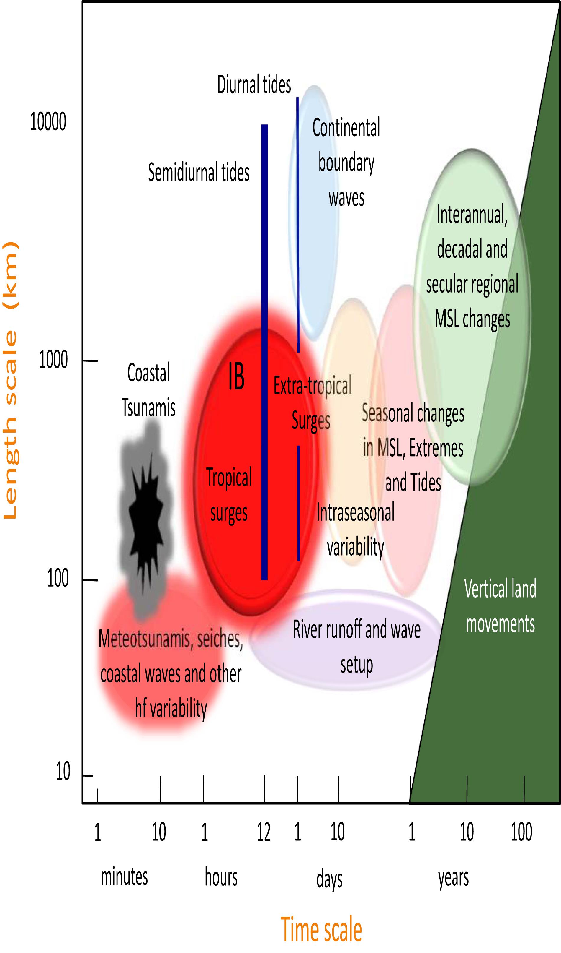
Figure 1. A schematic overview of processes contributing to sea level variability at the coast indicating the space and time scales involved. Woodworth et al. (2019) contains a more complete summary and discussion of each process; Hughes et al. (2019) provides a detailed review of different types of coastal-trapped waves. Very high-frequency processes with timescales less than 1 min (e.g., wind waves, swash) are not included.
In fact, some of these higher-frequency processes are important to the discussion of SL variability and change over longer timescales. For example, major periods of storm surge activity in winter will skew the distribution of surges and therefore affect monthly mean SL. Wave setup and run-up provides another example. While run-up is the instantaneous maximum elevation at the moving shoreline, wave setup is the SL averaged typically over many wave groups (tens of minutes). This wave setup is modulated on longer timescales through its dependence on time-varying wave height, period, direction, and “still water” level (Idier et al., 2019). Therefore, setup will inevitably contribute to mean SL variability in some way (e.g., on seasonal and interannual timescales). Consequently, there is a possible “contamination” of existing long term mean SL records by variations in wave setup in the past (IOC, 2016). In addition, the character of the contribution might change again if wind climate or sea ice cover changes in the future, leading to changes in the wave climate (Stopa et al., 2016; Melet et al., 2018). Similar remarks apply to river runoff, which is primarily a high-frequency process (e.g., daily) and yet can contribute to SL variability on seasonal and longer timescales at tide gauges located in or near to major river estuaries (Wijeratne et al., 2008; Piecuch et al., 2018a).
Coast-Ocean Comparison on Longer Timescales
Many studies have demonstrated that the differences between open-ocean and coastal SL variability are not confined to the “high-frequency” and “short spatial scale” of the previous section. A well-known example concerns the trapped coastal waves that propagate north and south along the Pacific coasts of the Americas, resulting in similar SL anomalies at all points along the coast (Enfield and Allen, 1980; Pugh and Woodworth, 2014). A similar situation occurs along Australian coasts, where much of the coherence in the north and west is related to El Niño (see references in White et al., 2014), and along the European coasts (e.g., Calafat et al., 2012). Another example is the coherence of variability in sub-surface pressure (akin to inverse-barometer corrected SL) at intra-annual timescales along continental shelf slopes (Hughes and Meredith, 2006).
The accumulation of several decades of satellite altimeter data made it possible to compare SL variability in the open ocean and that at the coast as measured by tide gauges. Differences in variability exist at some locations on monthly to interannual timescales (e.g., Vinogradov and Ponte, 2011). Such differences are of particular interest where they reflect the dynamics of the nearby ocean circulation, and especially of western boundary currents (e.g., Yin and Goddard, 2013; Sasaki et al., 2014; McCarthy et al., 2015). Further studies are needed (e.g., using re-tracked coastal altimetry products) to identify the relative contributions of measurement issues (e.g., contamination of the altimeter footprint, uncertainties in correction algorithms) and representation errors (e.g., coastally trapped circulations) to the observed differences between tide gauge and altimetry data.
The performance of ocean models (Calafat et al., 2014; Chepurin et al., 2014) and coupled climate models (Becker et al., 2016; Meyssignac et al., 2017b) in reproducing historical coastal SL changes observed by tide gauges is varied, with the models performing well for some regions and timescales, but poorly for others. Consequently, better understanding of model-data discrepancies, and in particular the faithfulness of models in simulating the processes mediating the relationship between coastal SL and large-scale ocean circulation, will be required to improve and add confidence to projections of future coastal SL change (see section “Existing Modeling Systems”).
Importance to Coastal SL of Climate Modes and Ocean Dynamics
The influence of the major modes of climate variability (e.g., El Niño-Southern Oscillation, North Atlantic Oscillation, Indian Ocean Dipole, Pacific Decadal Oscillation) can be seen in spatial patterns of SL variability both at the coast and in the ocean interior, and in both coastal mean and extreme SL (e.g., Menéndez and Woodworth, 2010; Barnard et al., 2015). These modes have basin-wide influence on SL at interannual-to-decadal timescales and have large impacts on coastal oceans through local wind forcing associated with climate modes and also remote influence from the ocean interior. For instance, interannual-to-decadal surface wind anomalies associated with El Niño and Indian Ocean Dipole induce eastward propagating oceanic equatorial Kelvin waves. Upon arriving at the eastern boundary, part of the energy propagates poleward as coastally trapped waves, affecting SL in a long distance along the coastlines of the eastern Pacific (e.g., Chelton and Enfield, 1986) and eastern Indian Ocean (e.g., Han et al., 2017, 2018). Eastern boundary SL is also affected at interannual to decadal timescales by variability in longshore winds associated with extratropical atmospheric centers of action related to climate modes (Calafat et al., 2013; Thompson et al., 2014).
At the western boundary, in regions where the shelf is broad (e.g., Mid-Atlantic Bight), circulations over the shelf can be distinct from the open ocean, large-scale (greater than Rossby radius) circulation (Brink, 1998). Open ocean currents flow along the isobaths, setting a barrier for cross-isobath flows and thus constrain the influence of remote forcing from the open ocean on coastal SL. The generation of cross-isobath currents must be through ageostrophic processes (e.g., external surface forcing, non-linearity, friction). By including variable rotation effects, however, some Rossby wave energy can cross isobaths and arrive at the western ocean boundary (Yang et al., 2013). Indeed, a coastal sea level signal which is derived from open ocean dynamics has been observed but with significantly reduced amplitude at the coast and a shift toward the equator (Higginson et al., 2015). Part of this effect has been explained theoretically, for an ocean with vertical sidewalls (Minobe et al., 2017). The extension to include a continental slope shows that the same kind of spatial shift and reduction in amplitude still occurs, but is enhanced to a degree that depends sensitively on resolution and friction (Wise et al., 2018). This effect can be understood as an influence of coastal-trapped waves on the propagation of signals between open-ocean and coastal regions; see Hughes et al. (2019) for a review.
The SL and temperature variability associated with climate modes can result in coastal impacts, such as flooding or coral bleaching around coastlines and low-lying coral islands (e.g., Dunne et al., 2012; Ezer and Atkinson, 2014; Barnard et al., 2015; Ampou et al., 2017; Schramek et al., 2018). Interpretation of correlations between climate modes and SL should be made carefully, as climate modes reflect statistical summaries of multivariate behavior in the climate system. They are useful constructs though not themselves primary drivers of SL change (e.g., Kenigson et al., 2018). Rather, such correlations often indicate a direct forcing of the ocean by the atmosphere, locally or remotely, by means of such mechanisms as the inverted barometer effect, storm surge, wind setup, Ekman transport, Rossby waves, or Sverdrup balance (Andres et al., 2013; Landerer and Volkov, 2013; Thompson and Mitchum, 2014; Piecuch et al., 2016; Calafat et al., 2018). It has also been proposed (e.g., along the Eastern United States) that coastal SL is causally linked to other components of the variable and changing climate system, such as subpolar ocean heat storage (Frederikse et al., 2017), the changing mass of the Greenland Ice Sheet (e.g., Davis and Vinogradova, 2017), changes to the Gulf Stream (Ezer et al., 2013) and Atlantic Meridional Overturning Circulation (Yin et al., 2009; Yin and Goddard, 2013), depending on timescale.
Global eddy-resolving models have revealed the strength of the intrinsic ocean variability, which spontaneously emerges from oceanic non-linearities without atmospheric variability or any air-sea coupling (Penduff et al., 2011; Sérazin et al., 2015, 2018). These signals have a chaotic character (i.e., their phase is random and not set by the atmosphere; Penduff et al., 2018), impact most oceanic fields such as SL, ocean heat content, overturning circulation (e.g., Zanna et al., 2018), can reach the scale of gyres and multiple decades, and may blur the detection of regional SL trends over periods of 30 years (Sérazin et al., 2016), and in particular over the altimetric period (Llovel et al., 2018). This phenomenon has mostly been studied in the open ocean, but ongoing research shows that it impacts the 1993–2015 trends of SL in certain coastal regions (e.g., Yellow Sea, Sea of Japan, Patagonian plateau), raising new issues for the understanding, detection and attribution of coastal SL change.
This stochastic variability is most strongly manifested in the mesoscale, which dominates SL variability in much of the ocean. However, the mesoscale is strongly suppressed by long continental slopes, leading to a decoupling between open ocean and shelf sea variability, especially in high latitudes and western boundaries (Hughes and Williams, 2010; Bingham and Hughes, 2012; Hughes et al., 2018, 2019). The result is that open ocean-shelf coupling only tends to occur on larger scales, though there is still a significant stochastic part derived from the integrated effect of the mesoscale. An exceptional example is the Caribbean Sea, where a basin mode (the Rossby Whistle) is excited by the mesoscale and has a strong influence on coastal SL at 120-day period (Hughes et al., 2016). Similarly, the short circumference of continental slopes around oceanic islands allows for the ready influence of mesoscale open ocean variability on their shorelines (Mitchum, 1995; Firing and Merrifield, 2004; Williams and Hughes, 2013).
Secular Coast-Ocean Differences
An obvious difference between coastal SL as seen by a tide gauge and open ocean SL as measured by an altimeter, which manifests itself primarily in the discussion of long-term SL trends, is that the former is made relative to land levels at the tide gauge stations, whereas the latter are referenced to the geocenter. Differences between the two SL measurements are rendered by VLMs, which can arise from a wide variety of processes (glacial isostatic adjustment, sediment compaction, tectonics, groundwater pumping, dam building) operating over a broad range of space and time scales (Emery and Aubrey, 1991; Engelhart and Horton, 2012; Kemp et al., 2014; Karegar et al., 2016; Johnson et al., 2018). Related bathymetric changes can also influence many coastal processes. Modern geodetic techniques are required to place the tide gauge data into the same geocentric reference frame as for the altimeter data, and to monitor VLM at the gauge sites (IOC, 2016; Wöppelmann and Marcos, 2016) and to understand as well as possible the evolution of coastal zones (Cazenave et al., 2017). Application of geodetic approaches in SL studies is limited currently by the spatial sparseness of the data, the temporal shortness of the records, and difficulties associated with realizing the terrestrial reference frame (cf. section “Sea Level Observations”).
Sea Level Change Impacts at the Coast
Major differences between ocean and coastal SL occur through processes that depend upon water depth, such as storm surges that lead to extreme SLs. A particular concern for coastal managers has to do with the extreme SLs and associated coastal inundation and flooding, that are occurring increasingly often (e.g., Sweet and Park, 2014). Extreme SL arises from combinations of high astronomical tides and other processes, in particular storm surges and waves (Merrifield et al., 2013). Changes in extremes have been found to be determined to a great extent by changes in mean SL, although not exclusively so (e.g., Marcos and Woodworth, 2017; Vousdoukas et al., 2018). These studies often make use of tide gauge data with its traditional hourly sampling of SL. Such sampling ignores the high-frequency part of the SL variability spectrum (timescale < 2 h, which includes most seiches), which should be accounted for, at least on a statistical basis, in future studies of extremes (Vilibić and Šepić, 2017). Also global scale studies of the impacts of sea level extremes do not include high-frequency wave-related processes such as swash.
However, the coast can also be impacted by changes in mean SL, which is known to be rising globally as a consequence of climate change (Church et al., 2013). The first years of altimeter data suggested that SL might be rising at a greater rate near to the coast than in the nearby deeper ocean (Holgate and Woodworth, 2004) although such a difference was not considered significant by others (White et al., 2005; Prandi et al., 2009). Nevertheless, as the depth of coastal waters increases in the future, many of the processes mentioned above will be modified: e.g., tidal wavelengths will increase and tidal patterns over the continental shelves will change (e.g., Idier et al., 2017); storm surge gradients and magnitudes will reduce (because of their dependence on 1/depth); changes to tides and surges imply changes to SL extremes; ocean waves will break closer to the coast, with associated changes in wave setup and run-up (Chini et al., 2010) and amplified potential flooding impacts (Arns et al., 2017). Many of these factors, as well as related morphological changes not discussed here, can be expected to interact with each other (Idier et al., 2019).
Summary: A Complexity of Coastal Processes
The nature of coastal SL variations is complex and multifaceted, reflecting the influence of a multitude of Earth system processes acting on timescales from seconds to centuries and on spatial scales from local to global. Successful efforts to monitor and predict coastal SL must acknowledge this complexity and deal with the challenges of observing many different variables, from local and remote winds and air pressure to river runoff and bathymetry, and modeling a wide range of processes, from wind waves, tides and large-scale climate modes, to compaction, sedimentation and tectonics affecting VLM (Figure 1).
Existing Observing Systems
Sea Level Observations
Tide gauges (Holgate et al., 2013) and satellite altimetry (Vignudelli et al., 2011; Cipollini et al., 2017a,b) are both important sources of SL information in the coastal zone. This section focuses on tide gauge observations and related systems. Benveniste et al. (2019) provide a discussion of coastal altimetry, including the complementarity between altimetry and tide gauge observations.
Coastal tide gauges measure point-wise water levels, from which mean and extreme SL can be estimated. The longest tide gauge records date back to the 18th century, although it was only during the mid-20th century that the number of instruments increased significantly, given their applications not only for scientific purposes but also for maritime navigation, harbor operations, and hazard forecasting. Currently, most of the world coastlines are monitored by tide gauges (Figure 2), generally operated by national and sub-national agencies. Many of these tide gauge records are compiled and freely distributed by international databases. Among these, the PSMSL1, hosted by the National Oceanography Centre in Liverpool, is the largest data bank of long-term monthly mean SL records for more than 2000 tide gauge stations (Holgate et al., 2013; see Figure 2). Other data portals provide higher frequency (hourly and higher) SL observations required for the study of tides and extreme SL and/or real time measurements needed for operational services or tsunami monitoring and warning systems; this is the case of the UHSLC2, the European Copernicus Marine Environment Monitoring Service3 or the Flanders Marine Institute4 that hosts the GLOSS monitoring facility for real time data. The Global Extreme Sea Level Analysis initiative5 extends the UHSLC high frequency SL data set, unifying and assembling delayed-mode observations compiled from national and sub-national agencies, and presently provides the most complete collection of high-frequency SL observations, with 1355 tide gauge records, of which 575 are longer than 20 years (Woodworth et al., 2017a).
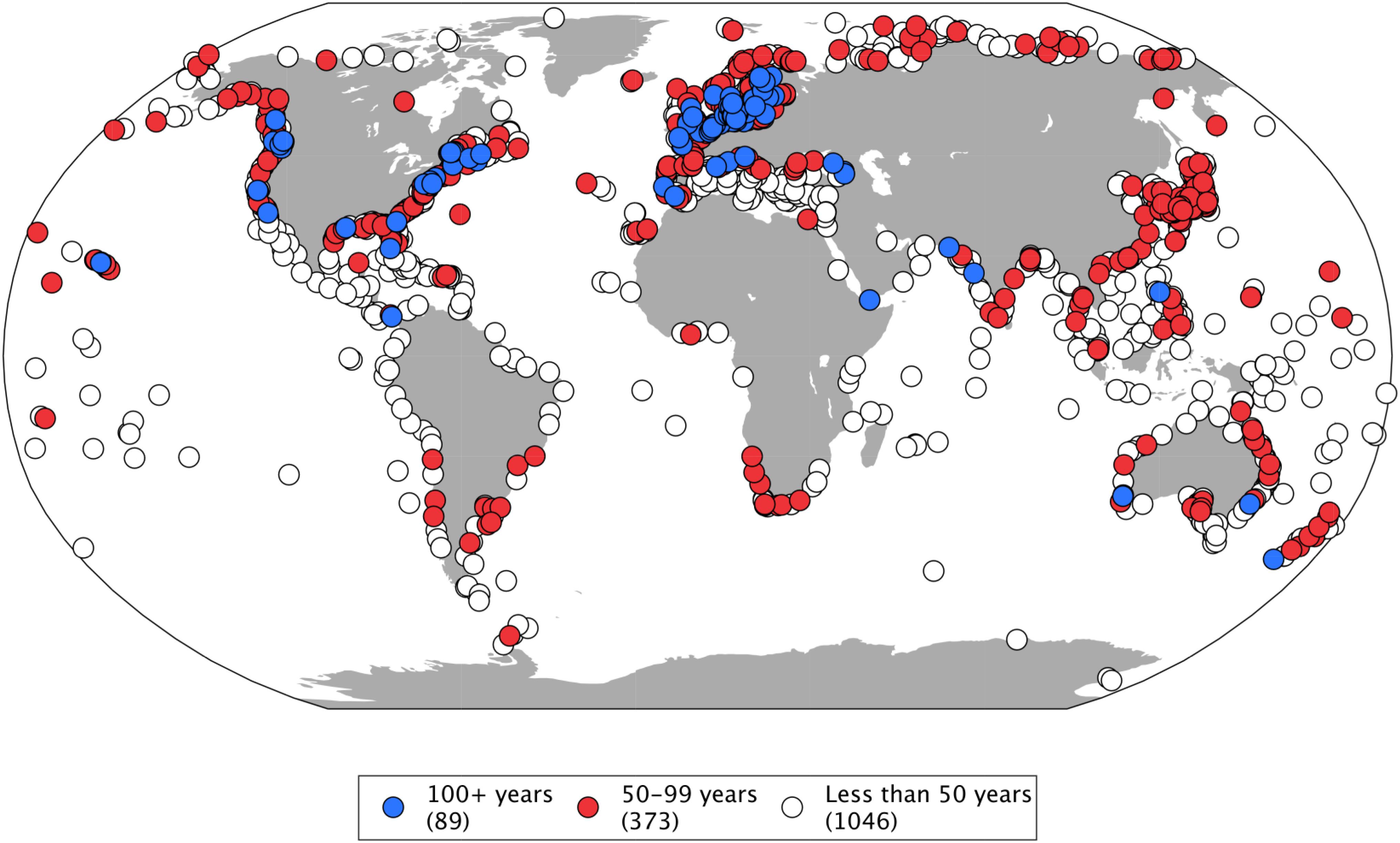
Figure 2. Tide gauge monthly sea level records available at PSMSL. In color, time series longer than 50 (red) and 100 (blue) years. Number of stations in each category is given in parentheses.
Despite the extensive present-day tide gauge network, only a fraction of the SL records spans a multi-decadal period necessary for climate studies. In the PSMSL data base, for example, only 270 (89) tide gauge records out of 1508 are longer than 60 (100) years – the minimum length considered by Douglas (1991) for the computation of linear trends – and only 632 overlap with altimetric observations during at least 15 years. Moreover, the longest tide gauge records tend to be located mostly in Europe and North America, while few are found in the Southern Hemisphere. This uneven spatial and temporal tide gauge distribution is one of the main factors that challenge the quantification and understanding of contemporary SL rise at regional and global scales (Jevrejeva et al., 2014; Dangendorf et al., 2017).
One of the tools to overcome the scarcity of coastal SL observations in the early 20th century and before, consists in the recovery and quality control of historical archived SL measurements, also referred to as data archeology (Bradshaw et al., 2015). These efforts have so far extended records from the PSMSL data set (Hogarth, 2014) and have successfully recovered new SL information at sites as remote as the Kerguelen Island (Testut et al., 2006) or the Falklands (Woodworth et al., 2010) and as far back in time as the 19th century (Marcos et al., 2011; Talke et al., 2014; Wöppelmann et al., 2014).
Tide gauges measure SL with respect to the land upon which they are grounded. Thus, to be useful for climate studies, tide gauge SL records must refer to a fixed datum, known as tide gauge benchmark, that ensures their consistency and continuity. Neither the land nor the SL are constant surfaces, so precise estimates of the VLM of the tide gauge benchmark are necessary in order to disentangle the climate contribution to SL change in tide gauge records. Presently, GNSS, with its most well-known component being the GPS, provide the most accurate way to estimate the VLM at the tide gauge benchmarks (Wöppelmann and Marcos, 2016). One major underlying assumption of the GPS-derived VLM at tide gauges is that the trend estimated from the shorter length of the GPS series is representative of the longer period covered by the tide gauge. When this is the case, GPS VLM reaches an accuracy one order of magnitude better than SL trends (Wöppelmann and Marcos, 2016). Another limitation is the accuracy of the reference frame on which the GPS velocities rely (Santamaría-Gómez et al., 2017). Global GPS velocity fields are routinely computed and distributed by different research institutions (International GNSS Service, Jet Propulsion Laboratory, University of Nevada, University of La Rochelle). Among these, only the French SONEL6 data center, hosted at the University of La Rochelle, provides GPS observations and velocity estimates focused on tide gauge stations, where possible providing links to PSMSL, to form an integrated observing system within the GLOSS program. Figure 3 maps the global tide gauge stations that are datum controlled and/or tied to a nearby GPS station for which VLM estimates exist. The number of tide gauge stations with co-located GPS is still a small fraction of the total network (e.g., only 394 stations in PSMSL are within a 10 km distance from a GPS station and, among these, only for 102 stations the leveling information between the two datums is available), despite recurrent GLOSS recommendations in this respect. The inability to account for VLM at tide gauges and therefore to separate the non-climate contribution of land from observed coastal SL, is another factor hampering the understanding of past SL rise.
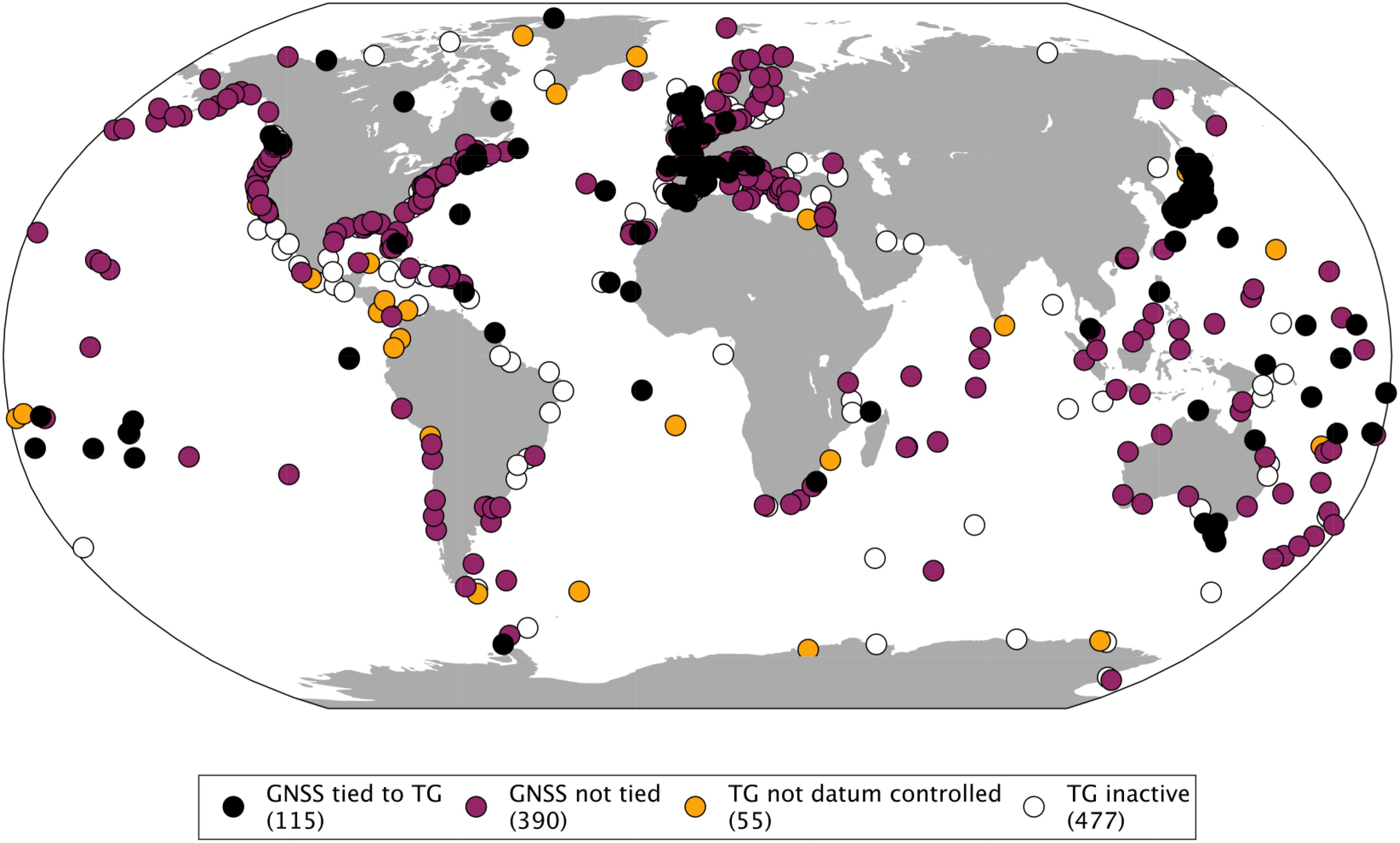
Figure 3. Tide gauges and collocated GPS. Number of stations in each category is given in parentheses.
As noted above, the continued deployment of GNSS receivers near or at tide gauges is critical. In this regard, a point also worth stressing concerns the actual placement of these systems: it is most useful if they are deployed so as to have an open view of the sea, thus allowing the measurement of both direct and reflected radio waves. The GNSS-reflectometry technique has proven that coastal GNSS stations can be used to supplement conventional tide gauges. Figure 4 compares 1 year-long time series of daily mean SL, produced from GPS reflections and from a standard acoustic tide gauge, with root-mean-square differences at the level of 2 cm (Larson et al., 2017). If installed in the vicinity of a tide gauge, GNSS receivers can provide a valuable backup as well as the direct tie between the tide gauge zero-point and the terrestrial reference frame (Santamaría-Gómez and Watson, 2017). There is no additional cost for developing new instrumentation, since standard geodetic-quality receivers can be used. However, data treatment is more complex than for a tide gauge and high frequency (daily) measurements are noisier in the case of a GNSS receiver.
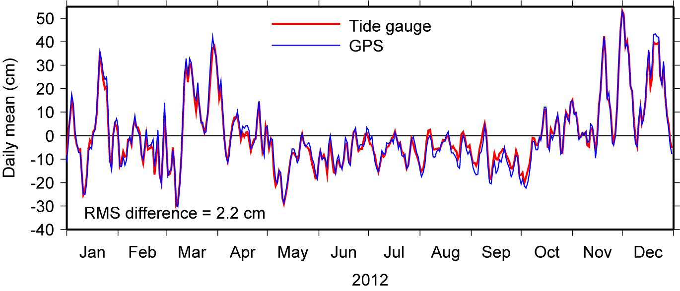
Figure 4. Daily mean sea level during 2012 at Friday Harbor, Washington, United States, in the Strait of Juan de Fuca. Red line is daily means deduced from the Friday Harbor tide gauge, operated by NOAA; blue line is daily means determined by analysis of GPS reflected signals at station SC02, sited 300 m from the tide gauge. Adapted from Larson et al. (2017), who give further comparisons over a 10-year period, including comparisons of tidal constants.
Ancillary Observations
The interpretation of coastal SL measurements benefits from complementary information provided by other ancillary observing systems focusing on various SL driving mechanisms and contributors. Among the components that impact coastal SL, wind-waves have a dominant role along many of the world coastlines acting at different timescales: from wave setup that modifies mean SL at the coast with timescales of a few hours, up to swash lasting only a few seconds. In the deep ocean, wind-waves are routinely monitored by in situ moored buoys, ship observations (Gulev et al., 2003) and satellite altimetry (Queffeulou, 2013). The offshore waves are strongly transformed in shallow waters owing to changing bathymetries and ocean bottom and thus display also large spatial variability even at small scales (∼10–100 m) along the coastal zone. Given the wide range of spatio-temporal scales, observations of wind-waves at the coast are generally recorded only at specific sites and target particular processes. Coastal wind-wave monitoring platforms include coastal pressure and wave-gauge deployments for near-shore waves, video monitoring techniques for shoreline positions (e.g., Holman and Stanley, 2007) and in situ field surveys for topo-bathymetries. Despite the impact that the topography and bathymetry of the surf zone have on wind-waves, lack of their routine measurement is currently one of the major gaps that limit the knowledge of wave transformations when approaching the coastal zone, especially in places with active seabed dynamics. This lack of information has also an effect on the ability of numerical models to predict both the coastal wave properties and the morphodynamical changes induced by their action. Given the impact of wind-waves on coastal SL, the inability to systematically observe coastal waves is a major knowledge gap.
Coastal SL is partly driven by changes in the deep ocean, where SL variations are largely due to water density (steric) changes (Meyssignac et al., 2017a). These signals are transferred to the coasts through a variety of mechanisms that depend on the open ocean circulation characteristics and on the physical processes taking place over the continental slope (e.g., Bingham and Hughes, 2012; Minobe et al., 2017; Calafat et al., 2018; Wise et al., 2018; see section “Causes of Coastal Sea Level Variability”). Therefore, observations of temperature and salinity in the open ocean, like those provided by the global Argo program, are also relevant to coastal SL. Unlike the deep ocean, density measurements are scarce over continental shelves, in enclosed or semi-enclosed basins and in the coastal zone. These measurements are generally obtained from dedicated field experiments or local/regional observing systems (e.g., Heslop et al., 2012; Rudnick et al., 2017) and are focused in areas of particular oceanographic interest (e.g., strong ocean currents, intense atmosphere-ocean interactions, fisheries). The hydrographic data scarcity in the shallow regions is a major hurdle to understand the small scale coastal dynamics and their impact on SL. On the other hand, sea surface temperature has shown covariability with SL along some coastal zones at interannual to decadal time scales, which is related to the fact that both are partly driven by air-sea heat fluxes (Meyssignac et al., 2017a). High-resolution, remote-sensed sea surface temperature can thus provide useful spatially detailed information for interpretation of SL features over the coastal zone (Marcos et al., 2019).
Ocean bottom pressure is another factor related to SL variability, especially over the continental shelves (e.g., Marcos and Tsimplis, 2007; Calafat et al., 2013; Piecuch and Ponte, 2015). Currently, satellite gravimetry, starting in 2002 with the launch of the GRACE mission, is the main source of observations of OBP changes over the deep ocean that allows separating the mass component from observed SL (Chambers et al., 2004). Available GRACE observations have relatively coarse resolution (∼300 km) and can be contaminated by leakage from larger land water fluctuations, but recent work by Piecuch et al. (2018b) highlights their usefulness in understanding the tide gauge records. Alternatively, OBP observations are also provided by in situ moored buoys. The largest network of OBP recorders is maintained and its data distributed by NOAA through the National Data Buoy Center website7. These OBP sensors display an uneven spatial distribution, as they are concentrated in areas of oceanographic interest or are part of tsunami warning systems, with most of them located in the deep ocean. OBP recorders are useful to quantify short-term ocean mass changes (Hughes et al., 2012), but they cannot be used to monitor long-term changes due to large internal drifts (Polster et al., 2009). The large-scale coherence of OBP signals along the continental shelves (Hughes and Meredith, 2006) suggests that they could be monitored with a relatively small network of in situ instruments, to overcome the currently limited set of OBP observations in coastal regions. However, this observational system does not exist so far at least on the global scale.
Monitoring and modeling of the main drivers of coastal SL variability (surface atmospheric winds and pressure, precipitation, evaporation, freshwater input at the coast from rivers and other sources), as well as other SL-related variables, is of course also essential. New observations have recently become available from remote sensing of wind speed, waves, SL and currents using X-band and high-frequency radar, acoustic Doppler current profilers, lidar, and Ku-band and Ka-band pulse-limited and delay Doppler radar altimetry, which promise high-quality space observations in the coastal zones (Fenoglio-Marc et al., 2015; Cipollini et al., 2017a,b). All these data are expected to improve forecasting model systems (Le Traon et al., 2015; Verrier et al., 2018). Observations relevant to the coastal forcing fields and other oceanic and atmospheric variables are discussed in a broader context by Ardhuin et al. (2019), Benveniste et al. (2019), and Cronin et al. (2019), among others.
Existing Modeling Systems
Modeling systems are essential for SL forecasts and projections. This section reviews the status of both regional model/data assimilation systems producing mostly short-term forecasts (order of days to weeks) and global coupled models used in long term climate projections. The discussion of the short-term forecast systems serves to highlight many issues of potential relevance (e.g., resolution, timescale interactions, data assimilation) for coastal SL prediction at the longer timescales as well.
Coastal Models and Sea Level Forecasts
In a very broad sense, a SL forecast can rely on three different approaches: (i) the use of realistic numerical models to resolve the processes that govern the ocean dynamics; (ii) the use of observations, which combined with statistical techniques are used to identify space and time patterns and extrapolate them into the future (e.g., linear regressions, ANN), and (iii) the hybrid approach, which combines the first two in a wide variety of ways. For instance, a given numerical model forecast can incorporate data assimilation to reduce the forecast errors and/or use an ensemble of forecasts to present the predictions with confidence intervals.
Kourafalou et al. (2015a,b) and De Mey-Frémaux et al. (2019) define a COFS as a combination of a comprehensive observational network and an appropriate modeling system that ensures the ongoing monitoring of changes in the coastal ocean and supports forecasting activities that can deliver useful and reliable ocean services. The Coastal Ocean and Shelf Seas Task Team within the Global Ocean Data Assimilation Experiment OceanView8 is an example of an effort that fosters the international coordination of these activities.
An adequate COFS should be able to monitor, predict and disseminate information about the coastal ocean state covering a wide range of coastal processes. These include: tides, storm surges, coastal-trapped waves, surface and internal waves, river plumes and estuarine processes, shelf dynamics, slope currents and shelf break exchanges, fronts, upwelling/downwelling and mesoscale and sub-mesoscale eddies. These variations occur over a wide range of time and space scales and have magnitudes of order 10–1–101 m (Figure 1).
The numerical models that integrate the primitive equations for solving the physical processes in a given COFS can vary in terms of complexity, from the more simplistic 2D shallow water equation models to the state-of-the-art 3D community models, such as the Regional Ocean Modeling System (ROMS9, Shchepetkin and McWilliams, 2005) and the Hybrid Coordinate Ocean Model (HYCOM10, Chassignet et al., 2003, 2007). While ROMS and HYCOM are based on a structured grid mesh, there is also a variety of models that use unstructured grids to facilitate an increase of resolution in areas of shallow or complex bathymetry. An example of such model is the Delft3D Flexible Mesh Suite11 or the Semi-implicit Cross-scale Hydroscience Integrated System Model (SCHISM)12. A table with some examples of COFS organized by region, maintained at https://www.godae-oceanview.org/science/task-teams/coastal-ocean-and-shelf-seas-tt/coss-tt-system-information-table/, illustrates the wide variety of models that can be used for this purpose. See also Fox-Kemper et al. (2019), which focuses on advances in ocean models and modeling.
Considering that the coastal ocean is both locally and remotely forced (e.g., Simpson and Sharples, 2012), a common adopted strategy is the use of a downscaling approach where remote forcing (e.g., large-scale currents and associated thermohaline gradients, tidal currents, swell) are incorporated in the COFS via initial and boundary conditions derived from coarser Ocean Forecasting Systems (see Tonani et al., 2015 for a worldwide list of such systems). The COFS forcing functions should represent all important shelf and coastal processes that influence SL, such as air-sea interaction, which close to coastal regions is affected by various time and space scales, and land-sea interaction, via coastal runoff, which governs buoyancy-driven currents that are further modified by the wind-driven circulation and shelf topography. An ideal COFS should include a robust data assimilation scheme capable of handling intrinsic anisotropy of the coastal region (Barth et al., 2007; Li et al., 2008; Tandeo et al., 2014; Stanev et al., 2016).
Several factors account for COFS uncertainties: imperfect atmospheric forcing fields; errors in boundary conditions propagating into the finer scale model domain; bathymetric errors; lack of horizontal and vertical resolution and numerical noise and bias; errors in parameterizations of atmosphere-ocean interactions and sub-grid turbulence; intrinsic limited model predictability (strong non-linearity), among many others. To improve prediction skill, data assimilation is used as a way of combining the results of numerical simulations with observations, so that an optimized representation of reality can be achieved. For this purpose, a range of algorithms is used in COFS such as the Optimal Interpolation (OI), the three-dimensional variational (3DVAR), the Ensemble Kalman Filter (EnKF), and the four-dimensional variational (4DVAR) data assimilation methods (Martin et al., 2015). The computational time involved in data assimilation can vary considerably based on the adopted algorithm and is also dependent on the chosen data assimilation cycle as well as the parameters that are assimilated in the COFS.
In analogy to the Earth System Models used in SL projections, COFS can also be coupled in many ways, such as atmosphere-to-ocean, wave-to-ocean and hydrology-to-ocean. As they are generally nested in regional and global models, COFS are particularly suited for coastal-offshore interactions and shelf break processes (provided that the nesting boundary is adequately offshore). An example of how coupling and a multi-nesting, downscaling approach can improve COFS quality is given by Staneva et al. (2016a). They employed a coupled wave-to-ocean model and three grids (horizontal resolutions of 3 nm, 1 km, and 200 m, Figure 5) to build a COFS capable of resolving non-linear feedback between strong currents and wind waves in coastal areas of the German Bight. Improved skill is demonstrated in the predicted SL and circulation during storm conditions when using a coupled wave-circulation model system (Staneva et al., 2017). During storm events, the ocean stress was significantly enhanced by the wind-wave interaction, leading to an increase in the estimated storm surge (compared to the ocean model only integration) and values closer to the observed water level (Figure 5B). The effects of the waves are more pronounced in the coastal area, where an increase in SL is observed (Staneva et al., 2016b). While maximum differences reached values of 10–15 cm during normal conditions, differences higher than 30 cm were found during the storm, along the whole German coast, exceeding half a meter in specific locations (Figure 5C).
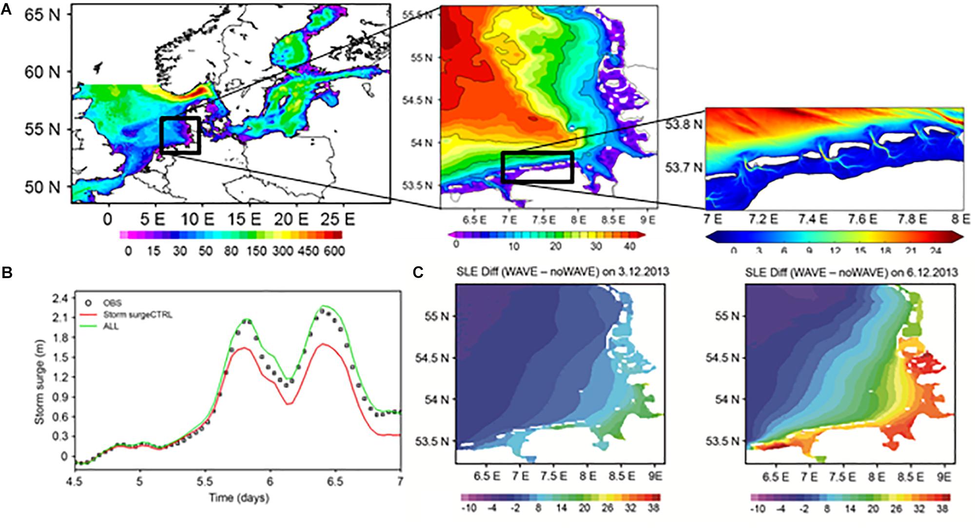
Figure 5. (A) Bathymetry of the nested grid model domains for the North Sea (left pattern), German Bight (middle pattern), and the east Wadden Sea (right pattern). The spatial resolution is 3 nm, 1 km, and 200 m, respectively. (B) Observed (black squares) against computed storm surges for the circulation model only (red line) and the coupled wave-circulation model (green line) during storm Xavier at station Helgoland. The X-axis corresponds to the time in days from December 1, 2013. (C) Sea level elevation (SLE) difference (cm) between the coupled wave–circulation model and circulation-only model for the German Bight on December 3, 2013 at 01:00 UTC (left) and during the storm Xavier on December 6, 2013 at 01:00 UTC (right). Adapted with permission from Staneva et al. (2016a, 2017).
Extreme events potentially associated with land falling hurricanes or extra-tropical storms can cause severe damage in coastal communities. In the US, operational guidance from storm surge and inundation models are used to inform emergency managers on whether or not to evacuate coastal regions ahead of storm events (Feyen et al., 2013). Kerr et al. (2013) investigated model response sensitivities to mesh resolution, topographical details, bottom friction formulations, the interaction of wind waves and circulation, and non-linear advection on tidal and hurricane surge and wave processes at the basin, shelf, wetland, and coastal channel scales within the Gulf of Mexico. Figure 6 presents their results based on two configurations of an unstructured-mesh, coupled wind-wave and circulation (shallow-water) modeling system, in a hindcast of Hurricane Ike that passed over the U.S. Gulf of Mexico coast in 2008. They show that the improved resolution is an important factor in predicting SL values much closer to those measured by the hydrographs.
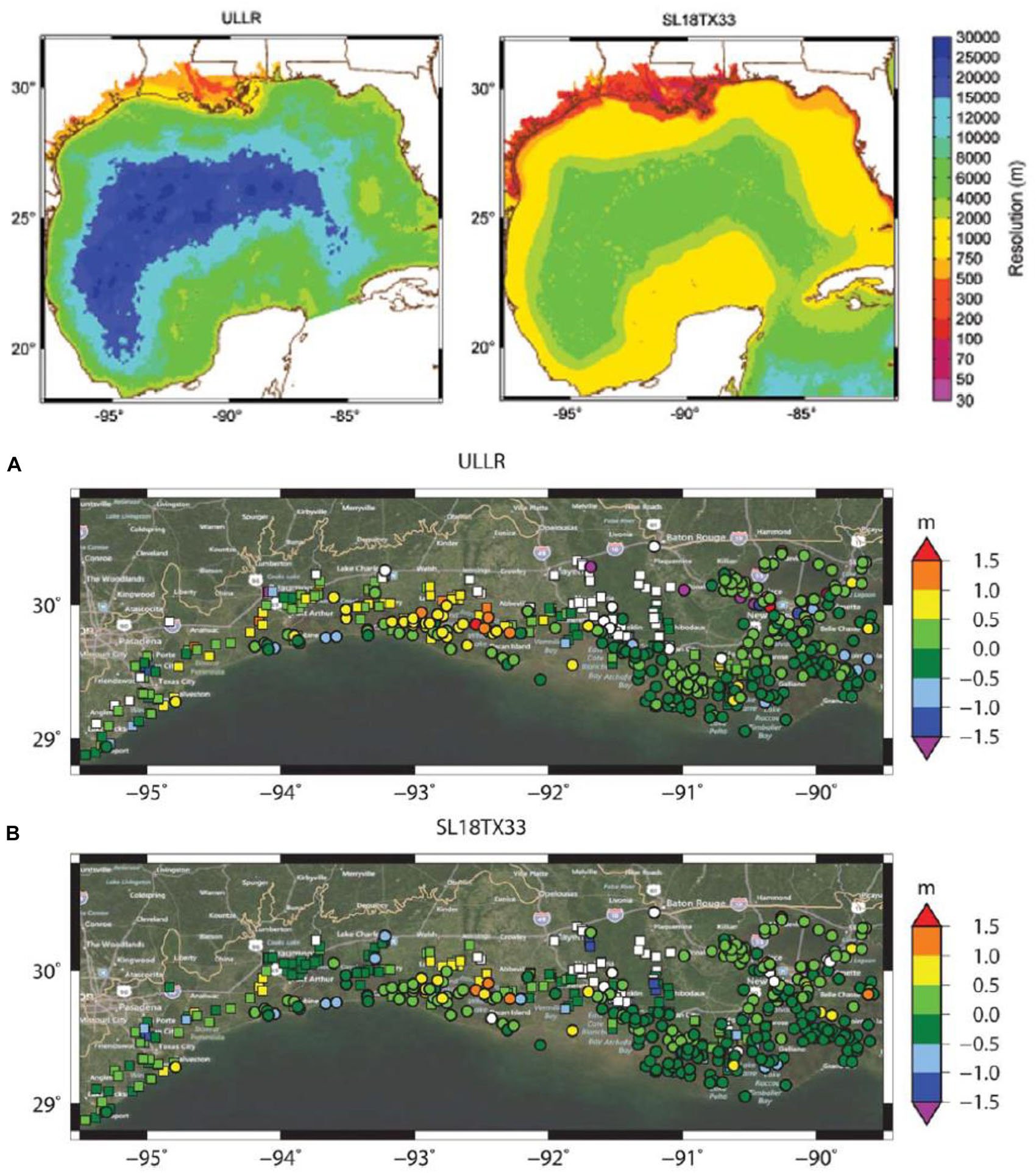
Figure 6. Top panels represent grid resolution in meters of two different model configurations for the Gulf of Mexico (lower resolution labeled ULLR; higher resolution labeled SL18TX33). Locations of Hurricane Ike peak water levels along the northwest Gulf Coast simulated by (A) ULLR and (B) SL18TX33 (circles), and measured by hydrographs (squares). The points are color-coded to show the errors between measured and modeled peak water levels. Green points indicate matches within 0.5 m and white points indicate locations that were never wetted by the model. Adapted with permission from Kerr et al. (2013).
The influence of strong boundary currents can also be important contributors for unusual SL changes. Usui et al. (2015) describe a case study to indicate the importance of a robust data assimilation scheme to accurately forecast an unusual tide event that occurred in September 2011 and caused flooding at several coastal areas south of Japan. Sea level rises on the order of 30 cm were observed at three tide-gauge stations and were associated with the passage of coastal trapped waves induced by a short-term fluctuation of the Kuroshio Current around (34°N, 140°E).
Probabilistic models have also been used alone or in conjunction with deterministic models for SL forecasts in various regions. Sztobryn (2003) used an ANN to forecast SL changes during a storm surge in a tideless region of the Baltic Sea where SL variations are pressure- and wind-driven. Bajo and Umgiesser (2010) used a combination of a hydrodynamic model and an ANN to improve the prediction of surges near Venice, in the Mediterranean Sea. French et al. (2017) combine ANN with computational hydrodynamics for tide surge inundation at estuarine ports in the United Kingdom to show that short-term forecast of extreme SL can achieve an accuracy that is comparable or better than the United Kingdom national tide surge model.
Climate Models and Sea Level Projections
Dynamic changes of the ocean circulation are the major source of regional SL variability in the open ocean (Yin, 2012; Church et al., 2013; Slangen et al., 2014; Jackson and Jevrejeva, 2016). Estimates of future dynamic SL variability, accounting for all contributions to regional SL change, are needed for understanding the magnitude, spatial patterns, and quality of regional to coastal SL projections.
Based on the CMIP5 ensemble, changes in interannual sea level variability from the historical modeled time frame 1951–2005 to the future modeled time frame 2081–2100 are mostly within ±10% for the RCP4.5 scenario, outside of the high-latitude Arctic region (Church et al., 2013). For decadal variability, Hu and Bates (2018) report that changes for period 2081–2100 are more consistently positive, and larger, over more of the ocean, and more so for RCP8.5 than RCP4.5, though this study uses a single model with a large ensemble.
Sources of inter-model uncertainty can be numerous, and include: model response to surface heat, freshwater, and wind forcing (Saenko et al., 2015; Gregory et al., 2016; Huber and Zanna, 2017); air-sea flux uncertainties, including fresh water fluxes (Stammer et al., 2011; Huber and Zanna, 2017; Zanna et al., 2018); different climate sensitivities (Melet and Meyssignac, 2015) and initial ocean states (Hu et al., 2017). Such intermodel uncertainty of regional SL change by 2090 can account for around 70% of total model uncertainty, including scenario uncertainty, meaning differences due to various RCP forcings, and the internal climate variability within individual models can account for approximately 5% of the total uncertainty for regional SL changes out to 2090 (Little et al., 2015). However, with these model uncertainties, changes in regional SL are larger than the total uncertainty by 2100, and pass the 90% significance level, for most ocean regions in both RCP4.5 and RCP8.5, whether trends are calculated for ocean-only processes that include global thermosteric SL change (Lyu et al., 2014; Richter and Marzeion, 2014; Carson et al., 2015; see Figure 7B), or for all forcing components of SL, including changes in land ice and water and global isostatic adjustment (Church et al., 2013; Lyu et al., 2014; see Figure 7C). Dynamic sea level changes alone emerge above the background variability only in high latitude regions, with few exceptions (Figure 7A), though there is substantial spread between models in the Southern Ocean (Figure 7D). The spread in the emergence time decreases everywhere when including changes in global thermosteric sea level (Figure 7E) and the other components of regional sea level change external to the climate models (Figure 7F). The coupled climate model changes in regional SL are larger than the noise (intermodel uncertainty, also called the ensemble spread, plus internal variability) in both the open ocean, and at the coast (Carson et al., under review). These model results are particularly due to the use of ensemble averaging to enhance the signal-to-noise ratio, though the uncertainty in dynamic SL between models is much larger than that due to internal model variability in 90–100-year trends (Little et al., 2015).
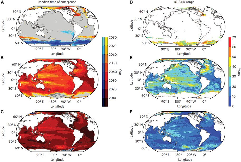
Figure 7. Time after which changes in local sea level are always larger than modeled local sea level variability (ensemble median) under RCP8.5, by year, for: (A) dynamic sea level, (B) dynamic plus global thermosteric sea level, and (C) all contributing components to regional sea level. Gray color means that no signal has yet emerged by 2080 or no agreement between models. The 16–84% uncertainty ranges at regions where at least 84% of the models in the ensemble show signal emergence by 2080 are shown in the right panels (D–F) for the same sea level change projection estimates (A–C). Adapted with permission from Figure 2 of Lyu et al. (2014).
Improvements in climate model physics and parameterizations that could reduce intermodel spread (for an exploration of causes of intermodel spread, see, e.g., Gregory et al., 2016) and better account for potential systematic errors in projected SL should be a goal of the international modeling community. However, the way forward in model improvement is complex. Clearly, some improvement can be found by increasing resolution, both for the atmosphere (Spence et al., 2014) and the ocean (Sérazin et al., 2015), especially in the context of SL changes in the vicinity of the Antarctic Circumpolar Current (Saenko et al., 2015) and Antarctic continental shelf (Spence et al., 2017); but, for some regions, SL projections seem to lack a strong sensitivity to resolution (Suzuki et al., 2005; Penduff et al., 2011). Another idea is to include only models in multi-model ensembles that have been proven to locally reproduce the physics of heat uptake and circulation changes due to wind and buoyancy forcing found in ocean observations – what has been termed climate model tuning (Mauritsen et al., 2012). Regional SL projections can be sensitive to the ocean model parameterizations used, although Huber and Zanna (2017) estimated that air-sea flux uncertainties were larger than those due to model parameterizations.
Although at relatively coarse resolution, CMIP5 simulations can capture expected features of coastal SL variability. For example, Minobe et al. (2017) explain some of the western boundary coastal SL change evident in most CMIP5 model projections via a theory which describes a balance between mass input to the western boundary due to Rossby waves from the ocean interior and equatorward mass ejection due to coastal-trapped wave propagation. There is, however, evidence that coastal SL projections are improved in higher resolution models (e.g., Balmaseda et al., 2015). For this reason, dynamical downscaling with regional climate models has been used to study the effects of climate change scenarios at the coast (e.g., Meier, 2006; Liu et al., 2016; Zhang et al., 2016, 2017). Global climate models are, however, generally used for providing boundary conditions to the higher resolution regional climate models, and uncertainties in those conditions can still be a problem.
Recommendations for Observing and Modeling Systems
Observational Needs
In this section, we examine tide gauge and related GNSS networks. Space-based SL measurements and other ancillary observations are considered in the papers cited at the end of section “Ancillary Observations.” The tide gauge and GNSS observing systems are mature and have clear oversight and procedures for setting requirements. Here we focus on identifying weaknesses in the present systems as opposed to setting additional requirements. The idea is that the requirements are well-known, but the weaknesses that need attention in the implementation of the systems are not as well-described.
Tide Gauges
Presently national entities voluntarily contribute their tide gauge data to the centers associated with the global network (GLOSS), from which it follows inevitably that there are gaps where national monitoring is either limited, absent, or not provided to GLOSS for some reason. Many efforts have been made to complete the global tide gauge network and to densify it on a regional basis, but these attempts have often been short-lived, and even after gauges have been installed successfully the essential ongoing maintenance thereafter has been lacking. For example, great efforts were made several years ago to install new gauges in Africa (Woodworth et al., 2007) but many of these gauges are no longer operational for various reasons.
More recently, the requirements for regional networks for tsunami warning (especially in the Indian Ocean and the Caribbean) and in support of other ocean hazards (e.g., hurricane-induced storm surges in the Caribbean) have led to an effective regional densification of the tide gauge network, but the improvements are patchy and sometimes come with compromises in measuring techniques. For example, some gauges used for tsunami monitoring do not have the requirement for excellent datum control that is needed for SL and coastal studies.
The present geographical gaps in tide gauge recording can be seen, e.g., in Figure 2, but it is important to recognize that there are gaps that are more subtle than those shown simply as dots on maps. For example, some operators employ outdated technology instead of the modern types of tide gauge (acoustic, pressure and, increasingly, radar) and the associated new data loggers and data transmission systems, which can provide accurate data in real time (IOC, 2016). In addition, some operators lack the technical expertise or resources required to operate their existing stations to GLOSS standards, in spite of GLOSS having put major efforts into capacity building through the years. In some countries, the tide gauges and the essential leveling to land benchmarks for datum control are the responsibility of different agencies, which may restrict communication between the responsible people (Woodworth et al., 2017b). In others, there is a lack of sufficient experts, generally university researchers specializing in oceanography, geodesy or SL science, who can make cogent arguments for tide gauges to local funding agencies. Other examples of gaps include major ports whose owners are content to use tide tables based on short historical records, instead of operating their own gauges to modern standards, which would enable the data to also be used for research. In addition, some old tide gauge records still remain non-digitized, despite their value for climate studies (Bradshaw et al., 2015).
One overarching gap is a lack of funding on both national and international levels. At the international level, it is imperative that we have regional network managers (1) to keep a close watch for gauges that are experiencing data outages or other problems, (2) to help with the installation of new gauges, and (3) to undertake the necessary leveling and other tasks where those activities fall between agencies. This applies especially to regions such as Africa where there are few people playing such roles on a national basis. The only real solution to this problem is the provision of central funding to the implementing group, which is presently GLOSS. At the national level, recent GLOSS-related workshops have demonstrated the major differences between the considerable investment in new tide gauge infrastructure in some countries and the lack of it in others (IOC, 2018). In some cases, national networks are being privatized, which is related to national funding, and this raises potential concerns about data quality and data sharing in the future (Pérez Gómez et al., 2017).
The satellite altimeter community considers in situ measurements by tide gauges to be an important source of complementary SL information (Roemmich et al., 2017). Such missions, which cost tens of millions of dollars USD each, have been secured as part of international cooperation involving most space agencies. Unfortunately, this is currently not the case for the global tide gauge network that they rely on, despite the fact the needs of such network are only a few million dollars per year.
GNSS Stations
As discussed in section “Sea Level Observations,” tide gauges are affected by VLM due to movements of the Earth’s crust where the gauges are attached. For many key SL applications (e.g., long-term climate studies or satellite altimetry drift estimation) the climatic and VLM contributions to the SL observations need to be separated, meaning that it is crucial to precisely and independently correct the VLM at the tide gauge locations. Since the early 1990s, GPS has been the only constellation suitable for precise VLM corrections (Carter, 1994; Foster, 2015), but nowadays other satellite positioning constellations such as GLONASS, Galileo, and BeiDou are also being considered.
Although associating a GNSS permanent station to a tide gauge has been required for the GLOSS network stations for some time (IOC, 2012), there is still work to do in terms of GNSS-tide gauge co-locations (King, 2014). Also, we should remember that the original idea behind the GLOSS initiative to use GNSS was to provide vertical positions and rates for the tide gauge benchmarks that are used to vertically reference the tide gauges (Carter, 1994). As the system evolved, however, the GNSS stations and the resulting VLM estimates were not always tied to the benchmarks and are therefore not directly related to the motion of the tide gauge zero point (Woodworth et al., 2017b). This prevents the absolute positioning of the tide gauges, and leaves questions as to the relevance of the GNSS VLM rates to the tide gauge zero point rates.
To be more specific, GNSS/tide gauge co-location data are provided in the SONEL databank (see text footnote 6), which is recognized as the GLOSS data center for GNSS. About 80% of the GLOSS tide gauges have a permanent GNSS station closer than 15 km (Figure 8), but many of these stations were not installed specifically for the monitoring of the tide gauge zero point, which explains why only 28% are closer than 500 m. This also explains the lack of direct ties to the tide gauge benchmarks mentioned above. This raises two issues. First, one cannot make a reliable geodetic link by conventional methods between the GNSS and tide gauge instruments when they are more than 1 km apart, which partly explains why only 29% of the GLOSS GNSS-co-located tide gauges have a geodetic tie available at SONEL. Second, if the GNSS and tide gauge zero point are not directly tied, then one must assume that the GNSS is measuring the same land movement that occurs at the tide gauge. Unless regular leveling campaigns are done between both instruments, this assumption is tenuous. Thus, we highly recommend that GNSS stations be installed as near as possible to the tide gauge site, and to carry out regular leveling campaigns when it is not.
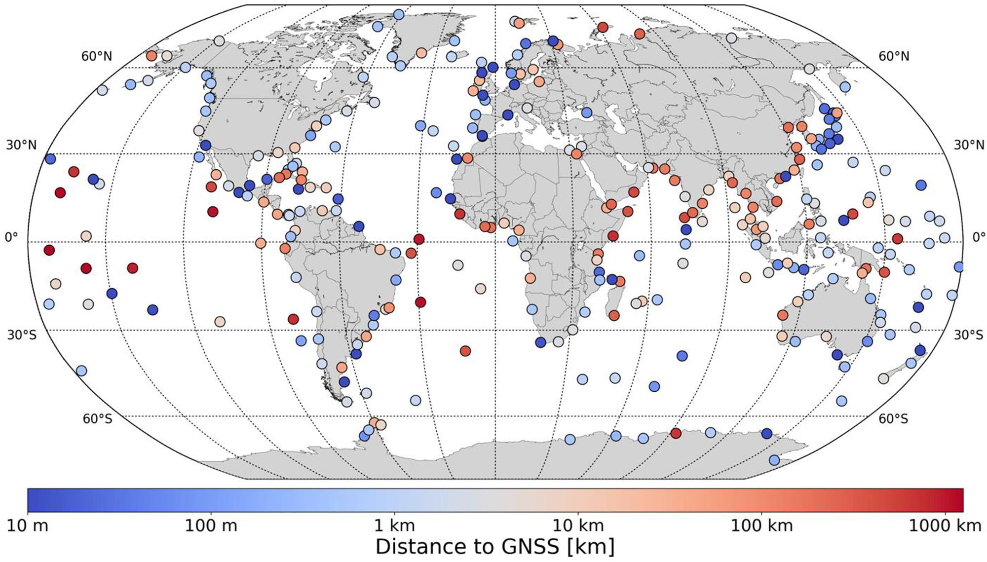
Figure 8. Distance between tide gauge and GNSS stations.
Finally, there is also an issue in terms of the VLM velocities that are available at present. There is currently one published GNSS solution dedicated to tide gauges, which was developed at the University of La Rochelle (Santamaría-Gómez et al., 2017), but other global velocity fields are available (Altamimi et al., 2016; Blewitt et al., 2016)13. For users, questions arises as to which solution to use, as these have substantial differences despite using essentially the same data. The GNSS VLM rates gain in accuracy when the data are processed by the largest number of analysis centers using different software and strategies, which is why it is crucial to make GNSS data freely available to the community. The International Association of Geodesy, through the Joint Working Group 3.2, currently focuses on constraining VLM at tide gauges by combining all the available global GPS VLM fields consistently into a single solution available to the sea-level community. This combined solution also allows examining the level of coherence between the different VLM estimates and their reproducibility by the different analysis centers.
Modeling Needs
Typical CMIP SL projections are a hybrid product, in the sense that some components (e.g., thermosteric changes) are an intrinsic part of CMIP simulations and others (e.g., SL changes related to land ice melt) are calculated off-line using CMIP output. The off-line calculations do not account for possible feedbacks in the climate system. In addition, for coastal projections, CMIP simulations are generally used only as boundary conditions for coastal forecasting models (e.g., Kopp et al., 2014).
An important part of projected SL trends on a regional scale arises from the dynamical and thermal and haline adjustment of the ocean related to changes in the circulation. On timescales up to decades, model improvements are needed to better capture the interannual variability of SL associated with climate modes discussed in section “Causes of Coastal Sea Level Variability” (e.g., Frankcombe et al., 2013; Carson et al., 2017). Simulations of such variability by climate models require further validation with emerging longer data sets of SL, mass or density changes.
At the same time, climate change also affects the cryosphere and terrestrial water storage, causing global mass changes in the ocean resulting in regional patterns (fingerprints) controlled by gravitational and rotational physics, as well as vertical motions of the sea floor (Slangen et al., 2014; Carson et al., 2016). For CMIP5 and before, these cryospheric/hydrologic changes were calculated off-line based on temperature and precipitation fields available from those coupled climate models (Church et al., 2013). The reasons to do so are manifold, as explained below.
If we consider the contribution from glaciers around the world, a key issue is that the spatial resolution that is required for glacier modeling is much finer than the spatial resolution of climate models. This mismatch is not easy to overcome and is therefore usually circumvented with off-line downscaling techniques, using as basic input the spatial and temporal variability from the climate models.
For the contribution of ice sheets, the required fine spatial scales remain an issue. The required scales for driving ice sheets are of the order 10 km and still smaller than what climate models typically resolve, though within reach of regional climate models. Some model experiments (Vizcaíno et al., 2013) show for instance that the surface mass balance of Greenland is reasonably well reproduced. Unfortunately, producing a reliable surface mass balance is only part of the problem, as forcing of the ice sheets is not only driven by the atmosphere but also by the ocean, particularly in Antarctica (Jenkins, 1991; Rignot et al., 2013; Lazeroms et al., 2018).
Changes in water mass characteristics on the continental shelves around Antarctica are generally believed to be the driving force behind the observed ice mass loss in West Antarctica (Joughin et al., 2014; Rignot et al., 2014). Warmer circumpolar water has likely led to increased basal melt rates forming the primary driver for changes in the area. Improved modeling of the basal melt rates in the cavities below the ice shelves requires first of all improved insight in the geometry of those cavities, and secondly very fine resolution ocean models to resolve the small-scale patterns controlling the water flow on the continental shelves. Nested ocean models may be a way forward as a complement to insights revealed from specialized fine resolution global models (e.g., Goddard et al., 2017; Spence et al., 2017).
Beside issues arising from the limited spatial resolutions of climate models, a second type of problem arises from the fact that the response timescales of ice sheets is far longer than for atmospheric processes and even significantly longer than for ocean processes. Hence initialization is a serious problem (Nowicki et al., 2016). This is specifically addressed by Goelzer et al. (2018) showing the wide variation in modeling results for the Greenland ice sheet depending on the initial shape and height of the present-day ice sheet. A way forward is to used remote sensing data that provides strong constraints on the mass loss over recent decades (Cazenave et al., 2018; Shepherd et al., 2018), which could constrain the dynamical imbalance of ice sheet models. Similarly, the dynamic state in terms of ice velocity as derived from InSAR observations can be used as a constraint to invert the spatially variable basal traction parameter (Morlighem et al., 2010). Several studies using data assimilation techniques (e.g., Seroussi et al., 2011) indicate that further improvements on the dynamical state are possible.
Finally, ice sheet models, which are generally believed to be the largest source of uncertainty on centennial timescales, are not yet integrated in climate models in part because our physical understanding remains limited. The grounding line physics controlling the boundary between the floating ice shelves and the grounded ice are now understood reasonably well (Pattyn et al., 2012). At the same time, it has become apparent that the stability of the ice sheet is not only dependent on the retrograde slope condition, underlying the classical marine ice sheet instability mechanism, but that the combination of hydrofracturing (Rott et al., 1996) and marine ice cliff instability (Bassis and Walker, 2012) may lead to a rapid disintegration of the ice sheet, as hypothesized by DeConto and Pollard (2016).
As a result of all the physically coupled, but currently poorly constrained processes associated with coupling of the ice sheets to climate models, fresh water fluxes produced by melting ice are not captured in the climate models (Bronselaer et al., 2018). This limitation might affect the circulation and sea ice formation in the Southern Ocean (e.g., Bintanja et al., 2013), which may feedback on the basal melt rates and accumulation on the ice sheet. Hosing experiments have been carried out in the past (Stouffer et al., 2006), but more refined fully coupled experiments are still needed.
Independent of improvements of coupling ice sheet and climate models, we have to consider improvements in the modeling skills of subsidence. This requires careful calibration of climate models, before they can be used as input for hydro-(geo)logical models, and additional assumptions on the socio-economic pathways not captured by the traditional climate model output. Full coupling seems out of the question due to spatial scale discrepancy between climate model and subsidence, but a more comprehensive aggregation seems feasible.
Beside improvements on regional SL projections as described above, there is a need to improve our projection skills with respect to near coastal conditions. Near the coast, SL projections are much more complicated because many small-scale dynamical processes (e.g., storm surges, tides, wind-waves, river runoff) and bathymetric features play a dominant role in determining extreme SL events and also affect longer period variability (see section “Causes of Coastal Sea Level Variability”). For this purpose, COFS (section “Coastal Models and Sea Level Forecasts”) need to be considered.
A main requirement for improving COFS for coastal SL is efficient downscaling techniques or nesting strategies. For example, Ranasinghe (2016) proposed a modeling framework for a local scale climate change impact quantification study on sandy coasts, starting from a global climate model ensemble, downscaled to regional climate model ensemble, which are then bias corrected and used to force regional scale coastal forcing models (waves, ocean dynamics, riverflows), which finally force local scale coastal impact models (such as Delft3D). Procedures include not only the assessment of the boundary conditions, but also the refinement of model set-ups, involving the grid, the topographic details and the various associated forcing, thereby addressing land-sea, air-sea, and coastal-offshore interactions (Kourafalou et al., 2015a,b). A realistic and detailed bathymetry is critical for COFS, since global models do not provide adequate coverage of shallow coastal areas and estuaries. As beaches are dynamic, changes in bathymetry should be explicitly modeled and include wetting and drying schemes (e.g., Warner et al., 2013). At the land-ocean interface, a particular challenge for forecasts of coastal SL changes and related circulation is the determination of realistic river inflows, since these values either come from river gauges, or from climatology or hydrological models. In addition to that, the correct representation of the river plume dynamics in COFS can also be challenging (e.g., Schiller and Kourafalou, 2010; Schiller et al., 2011). Further use of coupled modeling approaches is also important. For example, predicted surges can be significantly enhanced during extreme storm events when considering wave-current interactions (Staneva et al., 2016a, 2017).
Another promising avenue for improving the ability to project changes in extreme SL in coastal regions is the use of global, unstructured grid hydrodynamical models that can simulate extreme surge events (Muis et al., 2016), in combination with information on large-scale SL and atmospheric forcing available from CMIP-type calculations. This approach allows one to project changes in risk over time resulting from changes in both mean SL and extremes. In addition, improvements in projections of wave climate (Hemer et al., 2012; Morim et al., 2018) offer a possibility to better resolve changes in extremes caused by waves (Arns et al., 2017).
In the future, COFS can benefit substantially from improved data collection and availability, along with better characterization of measurement errors. For example, technological innovations such as Ka-band and SAR altimetry, as used in missions such as AltiKa and CryoSat-2, have contributed to the improvement of coastal altimetry techniques (Benveniste et al., 2019). Wide-swath altimetry promises further improvements (Morrow et al., 2019). Developments in many other data types (hydrography, bathymetry, coastal radar, coastal runoff, surface meteorology), discussed in other OceanObs’19 contributions, will all have an impact on the ability to forecast coastal SL. For any data type, it is important that the statistics of measurement errors (variances and covariances, dependences in space and time) be specified as best as possible, to be able to optimally inform the data assimilation systems.
Developing Future Sea Level Services
With more than 600 million people living in low elevation coastal areas less than 10 m above mean SL (McGranahan et al., 2007), and around 150 million people living within 1 m of the high tide level (Lichter et al., 2011), future SL rise is one of the most damaging aspects of a warming climate (Intergovernmental Panel on Climate Change [IPCC], 2013). Considering the 0.9 m global mean SL rise under RCP8.5 scenario, global annual flood costs without additional adaptation are projected to be US$ 14.3 trillion per year (2.5% of global GDP), and up to 10% of GDP for some countries (Jevrejeva et al., 2018). Adaptation could potentially reduce SL induced flood costs by a factor of 10 (Hinkel et al., 2014; Jevrejeva et al., 2018; Vousdoukas et al., 2018).
Global Sea Level is one of seven key indicators defined by the World Meteorological Organisation within the Global Climate Observing System Program to describe the changing climate. The importance of, as a minimum, maintaining existing SL observing systems cannot be overstated. More generally, the availability of coastal observations, scientific analysis and interpretation of such measurements, and future projections of SL rise in a warming climate are crucial for impact assessment, risk management, adaptation strategy and long-term decision making in coastal areas.
For risk assessment, decisions about adaptation to local SL rise, and resilience to coastal flooding, erosion and other changes in coastal areas, there is a need for SL services to support and empower stakeholders (e.g., governments, local authorities, coastal engineers, planners, socio-economists and coastal communities). In addition to existing climate services (e.g., those laid out in the report “A European research and innovation roadmap for climate services,” such as the Copernicus Climate Change Service)14, which ensure that climate research provides benefits and solutions to the challenges facing our society, there is an urgent necessity for specific equivalent expertise in coastal SL changes. An equivalent set of SL services could cover the transformation of data, together with other relevant information, into customized products such as projections, forecasts, information, trends, economic analysis, assessments (including technology assessment), counseling on best practices, development and evaluation of solutions and any other SL-related service that may be of use for the society at large.
To frame present status and future development of SL services that can address the challenges facing coastal communities, it is useful to consider the example of PSMSL (introduced in section “Existing Observing Systems”). Established in 1933, PSMSL is the global data bank for long term SL change information from tide gauges (Figure 2, section “Sea Level Observations”). Over the past few decades PSMSL has been providing the SL community with additional services relating to the acquisition, analysis, interpretation of SL data and a wide range of advice to tide gauge operators and data analysts.
With new challenges due to climate change and SL rise there is an urgent need worldwide to support decisions on managing exposure to climate variability and change. The PSMSL will address these needs by offering a range of services including expert advice, bespoke climate information, value added services and solutions to help build capacity in developing countries.
Using the expanding knowledge of climate and SL science, expertise in past and future SL changes, and a growing understanding of how climate hazards impact society and the environment, PSMSL is currently developing a new framework (including a set of products) that will be vital for empowering decision-makers in coastal cities, small island states and local communities to respond to the risks and opportunities of climate variability and change. With the main focus on developing countries, new PSMSL products (e.g., Figure 9) will support climate-smart decisions to make coastal societies more resilient to SL rise and climate change, and meet international capacity development objectives, ensuring that public investment in climate science can be used to maximum effect.
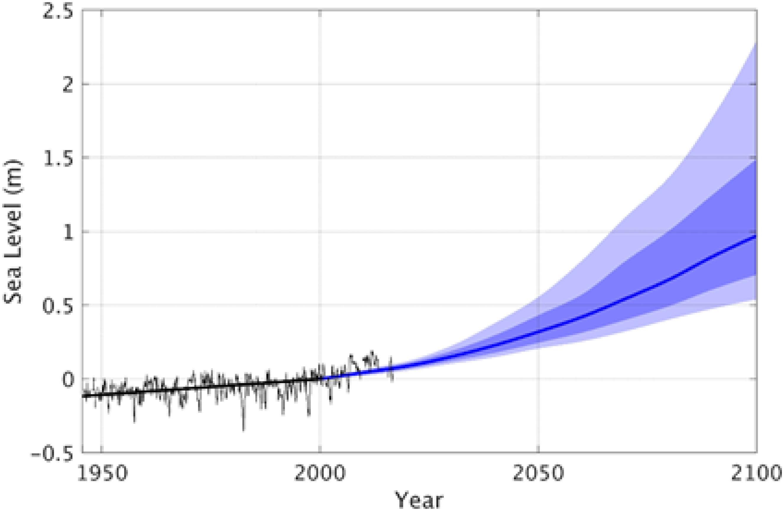
Figure 9. Tide gauge observations (black lines) combined with sea level projections (blue) with RCP 8.5 scenarios at Kwajalein, Marshall Islands (Jackson and Jevrejeva, 2016). The thin black line is monthly tide gauge record, the thick black line is long-term linear trend; the thick blue line is sea level projection at 50% probability, and the dark and light blue shading areas represent 17–83 and 5–95% probabilities, respectively.
The PSMSL has experience working with more than 200 data authorities and close co-operation with GLOSS/ Intergovernmental Oceanographic Commission/European Global Ocean Observing System, and therefore has the opportunity to take a world-leading role to develop and deliver a suite of SL services. For example, PSMSL already provides products15 globally, regionally and nationally and will develop these further, particularly drawing on its expertise to support decision-makers.
In addition to PSMSL, a variety of agencies and research groups have demonstrated leadership in this arena. In the United States, multiple frameworks have been developed to combine information about future SL rise with land-use, economic, and demographic data to inform decision makers and map regions of enhanced risk (e.g., NOAA’s Sea Level Rise Viewer16 ; Climate Central’s Risk Zone Map17). These frameworks can serve as examples on which to build services for other regions. As SL continues to rise and flooding events become more common, it will become increasingly important to develop tools that provide short-term forecasts of problematic coastal conditions. For example, UHSLC provides seasonal SL forecasts to Pacific Island communities (Figure 10)18, which combine output from state-of-the-art operational models with local tide predictions to give local stakeholders advanced notice of likely tidal flooding conditions. The web-based product is supplemented by an active email forecast discussion group with local weather services, and work is currently underway to expand to United States continental coastlines. At even shorter timescales of days to weeks, it is possible to forecast the gravity wave field of the ocean and, by extension, the impact of these waves on total water level at the coastline. The USGS Total Water Level and Coastal Change Forecast Viewer19 provides one example of how short-term forecasts of SL, tide, and waves can be combined to provide decision makers with comprehensive view of imminent conditions to drive science-supported action. These examples provide a basis for further development, but are by no means comprehensive. Providing necessary sea level services for all regions of need will require international collaboration and cooperation between research centers, national agencies, and local authorities.
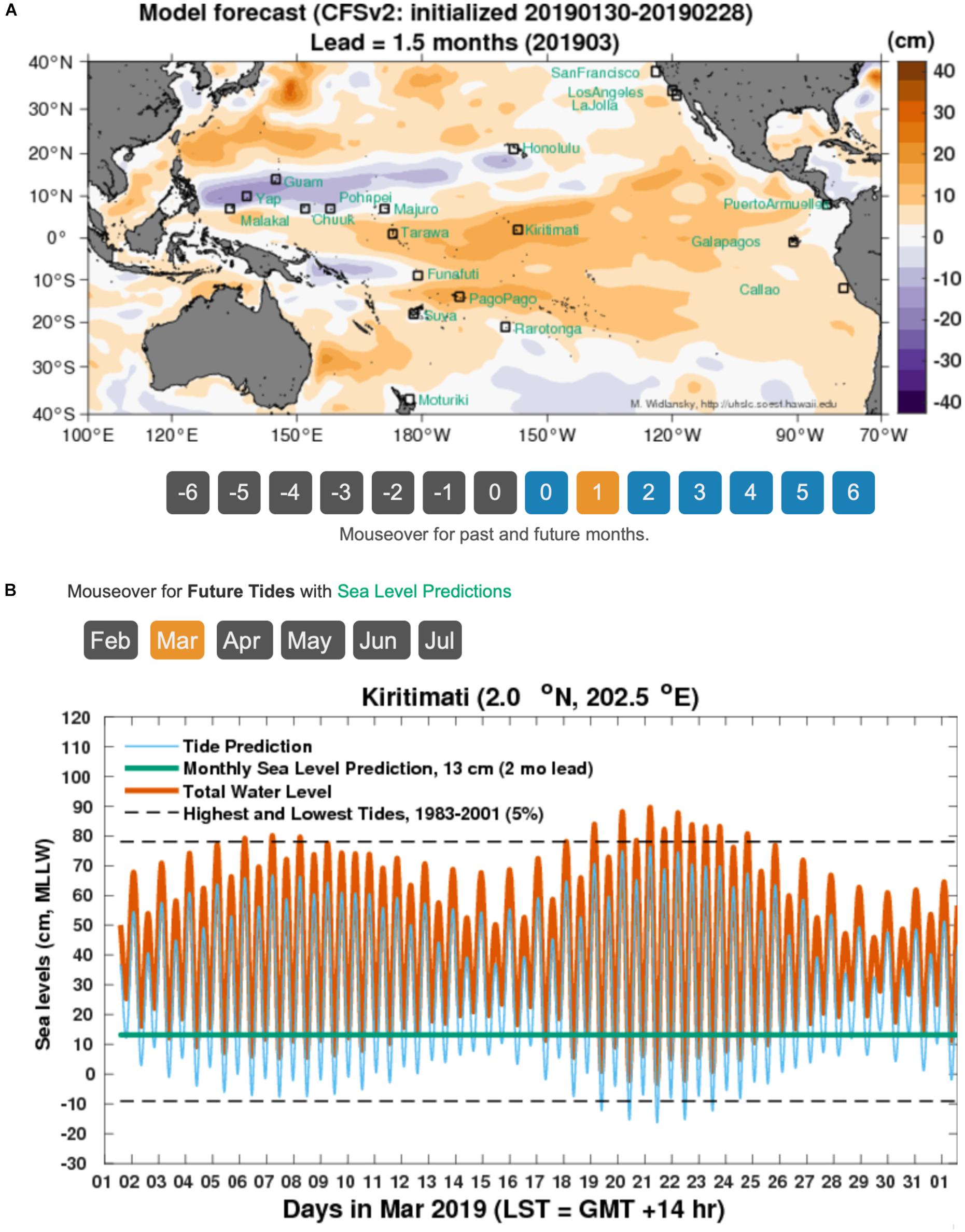
Figure 10. University of Hawai’i Sea Level Center’s seasonal forecast product of monthly mean sea level (Widlansky et al., 2017). (A) Sea level forecast for the tropical Pacific with 1 month lead from an operational forecast model. (B) Astronomical tide predictions plus forecasted mean sea level with 1 month lead for the island of Kiritimati. The combination of tides plus mean sea level provides a more accurate forecast of high tide and potential impacts compared to astronomical predictions alone.
Examples of continued and future developments include:
• Localized SL projections to inform local development and mitigation plans;
• Development of software capable of performing automatic quality control of tide gauge data;
• Low cost temporary tide gauges for surveys in remote areas;
• Identification of locally relevant flooding thresholds that identify specific elements of at-risk infrastructure;
• Regional storm surge and inundation forecasting.
The Sea Level Futures Conference (Liverpool, United Kingdom, July 2–4, 2018), celebrating the 85th anniversary of PSMSL, reviewed the present status of SL science knowledge, covering key aspects of SL change. Special emphasis was given to existing SL observations, synthesis of available data and discussion of future novel observational techniques in coastal areas. The science provides clear evidence that SL is rising and this is already impacting vulnerable coastal areas, especially those with rapidly growing urban populations and associated infrastructure. Addressing these challenges in a warming climate requires integrated sustainable and continued observations, data products and advanced modeling capability. Thus, as recognized by conference participants, there is a requirement for close collaboration between scientists from different disciplines and the broad stakeholder community to develop plans for responding to SL change, storm surges and flood risk affecting the coastal zone. Key actions necessary to enable the development of SL services that can effectively support adaptation and mitigation measures and empower decision-makers in coastal communities should include:
• Commitment to sustained, systematic and complementary global and coastal measurements of SL and its components to understand observed variability and change, to constrain longer term projections and to improve skill of forecasting and early warning systems. This commitment must be in line with efforts under the Global Ocean Observing System, Global Geodetic Observing System, GLOSS and other programs.
• Commitment to extend the historical SL record through data rescue, digitization and the accurate detailed integration of historic tide gauge data into international repositories to reduce spatial and temporal gaps and to validate process-understanding as well as process-based climate models, and to detect and attribute the influence of natural (intrinsic and externally forced) and human-induced drivers.
• Broad-scale assessment of uplift/subsidence, especially human-induced subsidence, to guide analysis of local SL change. The international community should take steps to provide all available information (e.g., from GNSS or InSAR) about uplift/subsidence in coastal areas. This work should involve the use of GNSS at all tide gauge stations (as per GLOSS standards) and the maintenance of an accurate International Terrestrial Reference Frame.
• Implementation of a multi-purpose approach to tide gauge networks, focusing on the requirements of all users (e.g., scientists, port authorities, coastal engineers and hazard forecasters), to ensure the sustainability of such networks. This is particularly important when establishing stations in developing economies (e.g., most of Africa), where existing networks tend to be deficient. Tide gauge measurements, including past records, are essential for improving our knowledge of coastal SL variability, which is one of the main gaps in SL science.
• Implementation of comprehensive observations in coastal areas, including expansion of in situ and satellite SL measurements, VLM, waves, sediment transport and relevant ancillary observations (e.g., bathymetry, river runoff), with special emphasis on monitoring changes in vulnerable coastal zones where a variety of climate and non-climate related processes interact (e.g., deltas, cities, small island states).
• Development of new technologies for SL observations on both coastal and global scales, e.g., low cost tide gauges and low cost GNSS units fitted to buoys/floating platforms, GNSS-reflectometry, coastal altimetry and wide-swath altimetry.
• Development of improved coastal SL projections and forecasts, involving dedicated data efforts for model advancement, exploration of new assimilation schemes and downscaling techniques, and accounting for the additional key processes at work in the coastal zone (e.g., tides, wave run-up, storm surges, river discharge).
• Quantitative assessment of uncertainties in all data streams, to improve monitoring activities and advance modeling and assimilation systems, and all SL projection and forecast products, along with clear understanding of different contributors to observed coastal SL variability and change (e.g., climate modes, intrinsic ocean fluctuations, anthropogenic forcing, VLM).
• Closer and wider cooperation between the scientific community, stakeholders, policy- and decision-makers to ensure that SL products are accessible and are used correctly and appropriately to facilitate adaptation and mitigation measures for vulnerable coastal areas (e.g., cities, deltas, small islands).
Author Contributions
This paper resulted from the merger, suggested by OceanObs’19 organizers, of three different abstracts led by RP, SJ, and GM. RP provided the original outline, coordinated the writing, and assembled the final paper. PW, MM, MCi, MCa, GM, RvdW, SJ, and CD led the writing of different sections, with input from CH, WH, AM, CP, TP, AS-G, DS, GW and others. All authors participated in the group discussions that led to the final contents of the manuscript.
Funding
RP was funded by NASA grant NNH16CT00C. CD was supported by the Australian Research Council (FT130101532 and DP 160103130), the Scientific Committee on Oceanic Research (SCOR) Working Group 148, funded by national SCOR committees and a grant to SCOR from the U.S. National Science Foundation (Grant OCE-1546580), and the Intergovernmental Oceanographic Commission of UNESCO/International Oceanographic Data and Information Exchange (IOC/IODE) IQuOD Steering Group. SJ was supported by the Natural Environmental Research Council under Grant Agreement No. NE/P01517/1 and by the EPSRC NEWTON Fund Sustainable Deltas Programme, Grant Number EP/R024537/1. RvdW received funding from NWO, Grant 866.13.001. WH was supported by NASA (NNX17AI63G and NNX17AH25G). CL was supported by NASA Grant NNH16CT01C. This work is a contribution to the PIRATE project funded by CNES (to TP). PT was supported by the NOAA Research Global Ocean Monitoring and Observing Program through its sponsorship of UHSLC (NA16NMF4320058). JS was supported by EU contract 730030 (call H2020-EO-2016, “CEASELESS”). JW was supported by EU Horizon 2020 Grant 633211, Atlantos.
Conflict of Interest Statement
RP and CL were employed by company Atmospheric and Environmental Research, Inc. MA was employed by company MAGELLIUM.
The remaining authors declare that the research was conducted in the absence of any commercial or financial relationships that could be construed as a potential conflict of interest.
Acknowledgments
The contents of this manuscript are partly based on the results from: the workshop on “Understanding the relationship between coastal sea level and large-scale ocean circulation,” held at and generously supported by the International Space Science Institute, Bern, Switzerland; the Sea Level Futures Conference, hosted by the National Oceanography Centre, Liverpool, United Kingdom; the project “Advanced Earth System Modelling Capacity,” and the Copernicus Marine Environmental Monitoring Service through the WaveFlow Service Evolution project.
Abbreviations
ANN, artificial neural networks; CMIP, Coupled Model Intercomparison Project; COFS, coastal ocean forecasting system; GLOSS, Global Sea Level Observing System; GNSS, Global Navigation Satellite System; GPS, Global Positioning System; InSAR, interferometric synthetic aperture radar; OBP, ocean bottom pressure; PSMSL, Permanent Service for Mean Sea Level; RCP, representative concentration pathway; SAR, synthetic aperture radar; SL, sea level; SONEL, Système d’Observations du Niveau des Eaux Littorales; UHSLC, University of Hawai’i Sea Level Center; VLM, vertical land motion.
Footnotes
- ^ https://www.psmsl.org
- ^ https://uhslc.soest.hawaii.edu/
- ^ http://marine.copernicus.eu/
- ^ http://www.vliz.be/en
- ^ https://www.gesla.org
- ^ http://www.sonel.org
- ^ http://www.ndbc.noaa.gov
- ^ https://www.godae-oceanview.org/
- ^ http://myroms.org
- ^ http://hycom.org
- ^ https://www.deltares.nl/en/software/delft3d-flexible-mesh-suite/
- ^ http://ccrm.vims.edu/schismweb
- ^ See also https://sideshow.jpl.nasa.gov/post/series.html
- ^ https://climate.copernicus.eu/
- ^ https://www.psmsl.org/products/
- ^ https://coast.noaa.gov/slr/
- ^ https://ss2.climatecentral.org/#12/
- ^ https://uhslc.soest.hawaii.edu/sea-level-forecasts/
- ^ https://coastal.er.usgs.gov/hurricanes/research/twlviewer/
References
Altamimi, Z., Rebischung, P., Métivier, L., and Xavier, C. (2016). ITRF2014: a new release of the International Terrestrial Reference Frame modeling nonlinear station motions. J. Geophys. Res. Solid Earth 121, 6109–6131. doi: 10.1002/2016JB013098
Ampou, E. E., Johan, O., Menkes, C. E., Niño, F., Birol, F., Ouillon, S., et al. (2017). Coral mortality induced by the 2015-2016 El-Niño event in Indonesia: the effect of rapid sea level fall. Biogeoscience 14, 817–826. doi: 10.5194/bg-14-817-2017
Andres, M., Gawarkiewicz, G. G., and Toole, J. M. (2013). Interannual sea level variability in the western North Atlantic: regional forcing and remote response. Geophys. Res. Lett. 40, 5915–5919. doi: 10.1002/2013GL058013
Ardhuin, F., Stopa, J. E., Chapron, B., Collard, F., Husson, R., Jensen, R. E., et al. (2019). Observing sea states. Front. Mar. Sci. 6:124. doi: 10.3389/fmars.2019.00124
Arns, A., Dangendorf, S., Jensen, J., Talke, S., Bender, J., and Pattiaratchi, C. (2017). Sea level rise induced amplification of coastal protection design heights. Sci. Rep. 7:40171. doi: 10.1038/srep40171
Bajo, M., and Umgiesser, G. (2010). Storm surge forecast through a combination of dynamic and neural network models. Ocean Model. 33, 1–9. doi: 10.1016/j.ocemod.2009.12.007
Balmaseda, M. A., Hernandez, F., Storto, A., Palmer, M. D., Alves, O., Shi, L., et al. (2015). The ocean reanalyses intercomparison project (ORA-IP). J. Oper. Oceanogr. 8, s80–s97. doi: 10.1080/1755876X.2015.1022329
Barnard, P. L., Short, A. D., Harley, M. D., Splinter, K. D., Vitousek, S., Turner, I. L., et al. (2015). Coastal vulnerability across the Pacific dominated by El Niño/Southern Oscillation. Nat. Geosci. 8, 801–807. doi: 10.1038/NGEO2539
Barth, A., Alvera-Azcárate, A., Beckers, J.-M., Rixen, M., and Vandenbulcke, L. (2007). Multigrid state vector for data assimilation in a two-way nested model of the Ligurian Sea. J. Mar. Syst. 65, 41–59. doi: 10.1016/j.jmarsys.2005.07.006
Bassis, J., and Walker, C. (2012). Upper and lower limits on the stability of calving glaciers from the yield strength envelope of ice. Proc. R. Soc. A. 468, 913–931. doi: 10.1098/rspa.2011.0422
Becker, M., Karpytchev, M., Marcos, M., Jevrejeva, S., and Lennartz-Sassink, S. (2016). Do climate models reproduce the complexity of observed sea level changes? Geophys. Res. Lett. 43, 5176–5184. doi: 10.1002/2016GL068971
Benveniste, J., Cazenave, A., Vignudelli, S., Fenoglio-Marc, L., Shah, R., Almar, R., et al. (2019). Requirements for a coastal zone observing system. Front. Mar. Sci. 6:348. doi: 10.3389/fmars.2019.00348
Bingham, R. J., and Hughes, C. W. (2012). Local diagnostics to estimate density-induced sea level variations over topography and along coastlines. J. Geophys. Res. 117:C01013. doi: 10.1029/2011JC007276
Bintanja, R., van Oldenborgh, G. J., Drijfhout, S. S., Wouters, B., and Katsman, C. A. (2013). Important role for ocean warming and increased ice-shelf melt in Antarctic sea-ice expansion. Nat. Geosci. 6, 376–379. doi: 10.1038/ngeo1767
Blewitt, G., Kreemer, C., Hammond, W. C., and Gazeaux, J. (2016). MIDAS robust trend estimator for accurate GPS station velocities without step detection. J. Geophys. Res. 121, 2054–2068. doi: 10.1002/2015JB012552
Bradshaw, E., Rickards, L., and Aarup, T. (2015). Sea level data archaeology and the Global Sea Level Observing System(GLOSS). Geophys. Res. J. 6, 9–16. doi: 10.1016/j.grj.2015.02.005
Brink, K. H. (1998). “Deep-sea forcing and exchange processes,” in The Sea, The Global Coastal Ocean: Processes and Methods, Vol. 10, eds K. H. Brink and A. R. Robinson (New York,NY: Wiley).
Bronselaer, B., Winton, M., Griffies, S. M., Hurlin, W. J., Rodgers, K. B., Sergienko, O. V., et al. (2018). Change in future climate due to Antarctic melting. Nature 564, 53–58. doi: 10.1038/s41586-018-0712-z
Calafat, F. M., Chambers, D. P., and Tsimplis, M. N. (2012). Mechanisms of decadal sea level variability in the eastern North Atlantic and the Mediterranean sea. J. Geophys. Res. 117:C09022. doi: 10.1029/2012JC008285
Calafat, F. M., Chambers, D. P., and Tsimplis, M. N. (2013). Inter-annual to decadal sea-level variability in the coastal zones of the Norwegian and Siberian seas: the role of atmospheric forcing. J. Geophys. Res. Oceans 118, 1287–1301. doi: 10.1002/jgrc.20106
Calafat, F. M., Chambers, D. P., and Tsimplis, M. N. (2014). On the ability of global sea level reconstructions to determine trends and variability. J. Geophys. Res. Oceans 119, 1572–1592. doi: 10.1002/2013JC009298
Calafat, F. M., Wahl, T., Lindsten, F., Williams, J., and Frajka-Williams, E. (2018). Coherent modulation of the sea-level annual cycle in the United States by Atlantic Rossby waves. Nat. Commun. 9:2571. doi: 10.1038/s41467-018-04898-y
Carson, M., Köhl, A., and Stammer, D. (2015). The impact of regional multidecadal and century-scale internal climate variability on sea level trends in CMIP5 models. J. Clim. 28, 853–861. doi: 10.1175/JCLI-D-14-00359.1
Carson, M., Köhl, A., Stammer, D., Meyssignac, B., Church, J., Schröter, J., et al. (2017). Regional sea level variability and trends, 1960–2007: a comparison of sea level reconstructions and Ocean syntheses. J. Geophys. Res. Oceans 122, 9068–9091. doi: 10.1002/2017JC012992
Carson, M., Köhl, A., Stammer, D., Slangen, A. B. A., Katsman, C., van de Wal, A. R. S. W., et al. (2016). Coastal sea level changes, observed, and projected during the 20th and 21st century. Clim. Change 134, 269–281. doi: 10.1007/s10584-015-1520-1
W. E. Carter (ed.) (1994). Report of the Surrey Workshop of the IAPSO Tide Gauge Bench Mark Fixing Committee. Report of a meeting held 13-15 December 1993 at the Institute of Oceanographic Sciences Deacon Laboratory. NOAA Technical Report NOSOES0006. Silver Spring, MD: NOAA, 81.
Cazenave, A., Ablain, M., Bamber, J., Barletta, V., Beckley, B., and Benveniste, J. (2018). Global Sea Level Budget 1993-present. Earth Syst. Sci. Data 10, 1551–1590. doi: 10.5194/essd-10-1551-2018
Cazenave, A., Le Cozannet, G., Benveniste, J., and Woodworth, P. (2017). Monitoring the Change of Coastal Zones from Space. Available at: https://eos.org/opinions/monitoring-coastal-zone-changes-from-space (accessed November 02, 2017).
Chambers, D. P., Wahr, J., and Nerem, R. S. (2004). Preliminary observations of global ocean mass variations with GRACE. Geophys. Res. Lett. 31:L13310. doi: 10.1029/2004GL020461
Chassignet, E. P., Hurlburt, H. E., Smedstad, O. M., Halliwell, G. R., Hogan, P. J., Wallcraft, A. J., et al. (2007). The HYCOM (Hybrid Coordinate Ocean Model) data assimilative system. J. Mar. Syst. 65, 60–83. doi: 10.1016/j.jmarsys.2005.09.016
Chassignet, E. P., Smith, L. T., and Halliwell, G. R. (2003). North Atlantic simulations with the hybrid coordinate ocean model (HYCOM): impact of the vertical coordinate choice, reference pressure and thermobaricity. J. Phys. Oceanogr. 33, 2504–2526.
Chelton, D. B., and Enfield, D. B. (1986). Ocean signals in tide gauge records. J. Geophys. Res. 91, 9081–9098. doi: 10.1029/JB091iB09p09081
Chepurin, G. A., Carton, J. A., and Leuliette, E. (2014). Sea level in ocean reanalyses and tide gauges. J. Geophys. Res. Oceans 119, 147–155. doi: 10.1002/2013JC009365
Chini, N., Stansby, P., Leake, J., Wolf, J., and Roberts-Jones, J. (2010). The impact of sea level rise and climate change on inshore wave climate: a case study for East Anglia (UK). Coast. Eng. 57, 973–984. doi: 10.1016/j.coastaleng.2010.05.009
Church, J. A., Clark, P. U., Cazenave, A., Gregory, J. M., Jevrejeva, S., Levermann, A., et al. (2013). “Sea Level Change,” in Climate Change 2013: The Physical Science Basis. Contribution of Working Group I to the Fifth Assessment Report of the Intergovernmental Panel on Climate Change, eds T. F. Stocker, D. Qin, G.-K. Plattner, M. Tignor, S. K. Allen, J. Boschung, et al. (Cambridge: Cambridge University Press).
Cipollini, P., Benveniste, J., Birol, F., Fernandes, M. J., Obligis, E., Passaro, M., et al. (2017a). “Satellite Altimetry in coastal regions,” in Satellite Altimetry Over Oceans and Land Surfaces: Earth Observation of Global Changes Book Series, eds D. Stammer and A. Cazenave (London: CRC Press), 644.
Cipollini, P., Calafat, F. M., Jevrejeva, S., Melet, A., and Prandi, P. (2017b). Monitoring sea level in the coastal zone with satellite altimetry and tide gauges. Surv. Geophys. 38, 33–57. doi: 10.1007/s10712-016-9392-0
Cronin, M. F., Gentemann, C. L., Edson, J., Ueki, I., Bourassa, M., Brown, S., et al. (2019). Air-sea fluxes with a focus on heat and momentum. Front. Mar. Sci. 6:430. doi: 10.3389/fmars.2019.00430
Dangendorf, S., Marcos, M., Woppelmann, G., Conrad, C. P., Frederikse, T., and Riva, R. (2017). Reassessment of 20th century global mean sea level rise. Proc. Natl. Acad. Sci. U.S.A. 114, 5946–5951. doi: 10.1073/pnas.1616007114
Davis, J. L., and Vinogradova, N. T. (2017). Causes of accelerating sea level on the East Coast of North America. Geophys. Res. Lett. 44, 5133–5141. doi: 10.1002/2017GL072845
De Mey-Frémaux, P., Ayoub, N., Barth, A., Brewin, B., Charria, G., Campuzano, F., et al. (2019). Model-observations synergy in the coastal ocean. Front. Mar. Sci. 6:436. doi: 10.3389/fmars.2019.00436
DeConto, R. M., and Pollard, D. (2016). Contribution of Antarctica to past and future sea level rise. Nature 531, 591–597. doi: 10.1038/nature17145
Douglas, B. C. (1991). Global sea level rise. J. Geophys. Res. 96, 6981–6992. doi: 10.1029/91JC00064
Dunne, R. P., Barbosa, S. M., and Woodworth, P. L. (2012). Contemporary sea level in the Chagos Archipelago, central Indian Ocean. Glob. Planet. Change 8, 25–37. doi: 10.1016/j.gloplacha.2011.11.009
Emery, K. O., and Aubrey, D. G. (1991). Sea Levels, Land Levels, and Tide Gauges. New York, NY: Springer-Verlag, 237.
Enfield, D. B., and Allen, J. S. (1980). On the structure and dynamics of monthly mean sea level anomalies along the Pacific coast of North and South America. J. Phys. Oceanogr. 10, 557–578. doi: 10.1175/1520-0485(1980)010<0557:otsado¿2.0.co;2
Engelhart, S. E., and Horton, B. P. (2012). Holocene sea level database for the Atlantic coast of the United States. Quat. Sci. Rev. 54, 12–25. doi: 10.1016/j.quascirev.2011.09.013
Ezer, T., and Atkinson, L. P. (2014). Accelerated flooding along the U.S. East Coast: on the impact of sea-level rise, tides, storms, the Gulf Stream, and the North Atlantic Oscillations. Earths Future 2, 362–382. doi: 10.1002/2014EF000252
Ezer, T., Atkinson, L. P., Corlett, W. B., and Blanco, J. L. (2013). Gulf Stream’s induced sea level rise and variability along the U.S. mid-Atlantic coast. J. Geophys. Res. 118, 685–697. doi: 10.1002/jgrc.20091
Fenoglio-Marc, L., Dinardo, S., Scharroo, R., Roland, A., Dutour, M., Lucas, B., et al. (2015). The German Bight: a validation of CryoSat-2 altimeter data in SAR mode. Adv. Space Res. 55, 2641–2656. doi: 10.1016/j.asr.2015.02.014
Feyen, J. C., Funakoshi, Y., van der Westhuysen, A. J., Earle, S., Caruso Magee, C., Tolman, H. L., et al. (2013). “Establishing a Community-Based Extratropical Storm Surge and Tide Model for NOAA’s Operational Forecasts for the Atlantic and Gulf Coasts,” in Proceedings of the 93rd AMS Annual Meeting, Austin, TX.
Firing, Y. L., and Merrifield, M. A. (2004). Extreme sea level events at Hawaii: influence of mesoscale eddies. Geophys. Res. Lett. 31:L24306. doi: 10.1029/2004GL021539
Foster, J. (2015). “GPS and surveying,” in Handbook of Sea-Level Research, eds I. Shennan, A. J. Long, and B. P. Horton (Hoboken, NJ: John Wiley & Sons), doi: 10.1002/9781118452547.ch10
Fox-Kemper, B., Adcroft, A. J., Boning, C. W., Chassignet, E. P., Curchitser, E., and Danabasoglu, G. (2019). Challenges and prospects in ocean circulation models. Front. Mar. Sci. 6:65. doi: 10.3389/fmars.2019.00065
Frankcombe, L. M., Spence, P., Hogg, A. M. C., England, M. H., and Griffies, S. M. (2013). ). Sea level changes forced by Southern Ocean winds. Geophys. Res. Lett. 457, 5710–5715. doi: 10.1002/2013GL058104
Frederikse, T., Simon, K., Katsman, C. A., and Riva, R. (2017). The sea-level budget along the Northwest Atlantic coast: GIA, mass changes, and large-scale ocean dynamics. J. Geophys. Res. Oceans 122, 5486–5501. doi: 10.1002/2017JC012699
French, J., Mawdsley, E., Fujiyama, T., and Achuthan, K. (2017). Combining machine learning with computational hydrodynamics for prediction of tidal surge inundation at estuarine ports. Procedia IUTAM 25, 28–35. doi: 10.1016/j.piutam.2017.09.005
Goddard, P., Dufour, C. O., Yin, J., Griffies, S. M., and Winton, M. (2017). CO2-induced ocean warming around the Antarctic ice sheet in an eddying global climate model. J. Geophys. Res.. 122, 8079–8101. doi: 10.1002/2017JC012849
Goelzer, H., Nowicki, S., Edwards, T., Beckley, M., Abe-Ouchi, A., and Aschwanden, A. (2018). Design and results of the ice sheet model initialization experiments initMIP-Greenland: an ISMIP6 intercomparison. Cryosphere 12, 1433–1460. doi: 10.5194/tc-12-1433-2018
Gregory, J. M., Bouttes, N., Griffies, S. M., Haak, H., Hurlin, W., Jungclaus, J., et al. (2016). The Flux-Anomaly-Forced Model Intercomparison Project (FAFMIP) contribution to CMIP6: investigation of sea-level and ocean climate change in response to CO2 forcing. Geosci. Model Dev. 9, 3993–4017. doi: 10.5194/gmd-9-3993-2016
Gregory, J. M., Griffies, S. M., Hughes, C. W., Lowe, J. A., Church, J. A., Fukumori, I., et al. (2019). Concepts and terminology for sea level–mean, variability and change, both local and global. Surv. Geophys. doi: 10.1007/s10712-019-09525-z
Gulev, S. K., Grigorieva, V., Sterl, A., and Woolf, D. (2003). Assessment of the reliability of wave observations from voluntary observing ships: insights from the validation of a global wind wave climatology based on voluntary observing ship data. J. Geophys. Res. 108:3236. doi: 10.1029/2002JC001437
Han, W., Meehl, G. A., Hu, A., Zheng, J., Kenigson, J., and Vialard, J. (2017). Decadal variability of indian and pacific walker cells: do they co-vary on decadal timescales? J. Clim. 30, 8447–8468. doi: 10.1175/JCLI-D-16-0783.1
Han, W., Stammer, D., Meehl, G. A., Hu, A., Sienz, F., and Zhang, L. (2018). Multi-decadal trend and decadal variability of the regional sea level over the indian ocean since the 1960s: roles of climate modes and external forcing. Climate 6:51. doi: 10.3390/cli6020051
Hemer, M. A., Wang, X. L., Weisse, R., and Swail, V. R. (2012). Advancing wind-waves climate science: the COWCLIP project. Bull. Am. Meteorol. Soc. 93, 791–796. doi: 10.1175/BAMS-D-11-00184.1
Heslop, E. E., Ruiz, S., Allen, J., López-Jurado, J. L., Renault, L., and Tintoré, J. (2012). Autonomous underwater gliders monitoring variability at “choke points” in our ocean system: a case study in the Western Mediterranean Sea. Geophys. Res. Lett. 39:L20604. doi: 10.1029/2012GL053717
Higginson, S., Thompson, K. R., Woodworth, P. L., and Hughes, C. W. (2015). The tilt of mean sea level along the east coast of North America. Geophys. Res. Lett. 42, 1471–1479. doi: 10.1002/2015GL063186
Hinkel, J., Lincke, D., Vafeidis, A. T., Perrette, M., Nicholls, R. J., Tol, R. S. J., et al. (2014). Future coastal flood damage and adaptation costs. Proc. Natl. Acad. Sci. U.S.A. 111, 3292–3297. doi: 10.1073/pnas.1222469111
Hogarth, P. (2014). Preliminary analysis of acceleration of sea level rise through the twentieth century using extended tide gauge data sets (August 2014). J. Geophys. Res. Oceans 119, 7645–7659. doi: 10.1002/2014JC009976
Holgate, S. J., Matthews, A., Woodworth, P. L., Rickards, L. J., Tamisiea, M. E., Bradshaw, E., et al. (2013). New data systems and products at the Permanent Service for Mean Sea Level. J. Coast. Res. 29, 493–504. doi: 10.2112/JCOASTRES-D-12-00175.1
Holgate, S. J., and Woodworth, P. L. (2004). Evidence for enhanced coastal sea level rise during the 1990s. Geophys. Res. Lett. 31:L07305. doi: 10.1029/2004GL019626
Holman, R. A., and Stanley, J. (2007). The history and technical capabilities of Argus. Coast. Eng. 54, 477–491. doi: 10.1016/j.coastaleng.2007.01.003
Hu, A., and Bates, S. C. (2018). Internal climate variability and projected future regional steric and dynamic sea level rise. Nat. Comm. 9:1068. doi: 10.1038/s41467-018-03474-8
Hu, A., Meehl, G. A., Stammer, D., Han, W., and Strand, W. G. (2017). Role of perturbing ocean initial condition in simulated regional sea level change. Water 9:402. doi: 10.3390/w9060401
Huber, M. B., and Zanna, L. (2017). Drivers of uncertainty in simulated ocean circulation and heat uptake. Geophys. Res. Lett. 44, 1402–1413. doi: 10.1002/2016GL071587
Hughes, C. W., Fukumori, I., Griffies, S. M., Huthnance, J. M., Minobe, S., Spence, J. P., et al. (2019). Sea level and the role of coastal trapped waves in mediating the interaction between the coast and open ocean. Surv. Geophys. doi: 10.1007/s10712-019-09535-x
Hughes, C. W., and Meredith, M. P. (2006). Coherent sea-level fluctuations along the global continental slope. Philos. Trans. R. Soc. A 364, 885–901. doi: 10.1098/rsta.2006.1744
Hughes, C. W., Tamisiea, M. E., Bingham, R. J., and Williams, J. (2012). Weighing the ocean: using a single mooring to measure changes in the mass of the ocean. Geophys. Res. Lett. 39:L17602. doi: 10.1029/2012GL052935
Hughes, C. W., Williams, J., Blaker, A., Coward, A., and Stepanov, V. (2018). A window on the deep ocean: the special value of ocean bottom pressure for monitoring the large-scale, deep-ocean circulation. Progr. Oceanogr. 161, 19–46. doi: 10.1016/j.pocean.2018.01.011
Hughes, C. W., Williams, J., Hibbert, A., Boening, C., and Oram, J. (2016). A Rossby whistle: a resonant basin mode observed in the Caribbean Sea. Geophys. Res. Lett. 43, 7036–7043. doi: 10.1002/2016GL069573
Hughes, C. W., and Williams, S. D. P. (2010). The color of sea level: importance of spatial variations in spectral shape for assessing the significance of trends. J. Geophys. Res. 115:C10048. doi: 10.1029/2010JC006102
Idier, D., Bertin, X., Thompson, P., and Pickering, M. D. (2019). Interactions between mean sea level, tide, surge, waves and flooding: mechanisms and contributions to sea level variations at the coast. Surv. Geophys. doi: 10.1007/s10712-019-09549-5
Idier, D., Paris, F., Le Cozannet, G., Boulahya, F., and Dumas, F. (2017). Sea-level rise impacts on the tides of the European Shelf. Cont. Shelf Res. 137, 56–71. doi: 10.1016/j.csr.2017.01.007
IOC (2012). The Global Sea Level Observing System (GLOSS) Implementation Plan - 2012. UNESCO/Intergovernmental Oceanographic Commission. IOC Technical Series No. 100. Paris: IOC, 37.
IOC (2016). Manual on Sea-level Measurements and Interpretation, Volume V: Radar Gauges. Paris, Intergovernmental Oceanographic Commission of UNESCO. IOC Manuals and Guides No.14, vol. V; JCOMM Technical Report No. 89. Paris: IOC, 104.
IOC (2018). Workshop on Sea-Level Measurements in Hostile Conditions, Moscow, Russian Federation, 13-15 March 2018. Intergovernmental Oceanographic Commission of UNESCO. IOC Workshop Reports, 281. Paris: UNESCO, 28.
Intergovernmental Panel on Climate Change [IPCC] (2013). “Intergovernmental Panel on Climate Change (IPCC) Summary for policymakers,” in Climate Change 2013: The Physical Science Basis. Contribution of Working Group I to the Fifth Assessment Report of the Intergovernmental Panel on Climate Change, eds T. F. Stocker, D. Qin, G.-K. Plattner, M. Tignor, S. K. Allen, J. Boschung, et al. (Cambridge: Cambridge University Press).
Intergovernmental Panel on Climate Change [IPCC] (2014). Climate Change 2014: Impacts, Adaptation, and Vulnerability. Summaries, Frequently Asked Questions, and Cross-Chapter Boxes. A Contribution of Working Group II to the Fifth Assessment Report of the Intergovernmental Panel on Climate Change, eds C. B. Field, V. R. Barros, D. J. Dokken, K. J. Mach, M. D. Mastrandrea, T. E. Bilir, et al. (Geneva: World Meteorological Organization), 190.
Jackson, L. P., and Jevrejeva, S. (2016). A probabilistic approach to 21st century regional sea-level projections using RCP and High-end scenarios. Glob. Planet. Change 146, 179–189. doi: 10.1016/j.gloplacha.2016.10.006
Jenkins, A. (1991). A one-dimensional model of ice shelf-ocean interaction. J. Geophys. Res.-Oceans 96, 20671–20677. doi: 10.1029/91JC01842
Jevrejeva, S., Jackson, L. P., Grinsted, A., Lincke, D., and Marzeion, B. (2018). Flood damage costs under the sea level rise with warming of 1.5 °C and 2 °C. Environ. Res. Lett. 13:074014. doi: 10.1088/1748-9326/aacc76
Jevrejeva, S., Moore, J. C., Grinsted, A., Matthews, A. P., and Spada, G. (2014). Trends and acceleration in global and regional sea levels since 1807. Glob. Planet. Change 113, 11–22. doi: 10.1016/j.gloplacha.2013.12.004
Johnson, C. S., Miller, K. G., Browning, J. V., Kopp, R. E., Kahn, N. E., Fan, Y., et al. (2018). The role of sediment compaction and groundwater withdrawal in local sea-level rise, Sandy Hook, New Jersey, USA. Quat. Sci. Rev. 181, 30–42. doi: 10.1016/j.quascirev.2017.11.031
Joughin, I., Smith, B. E., and Medley, B. (2014). Marine ice sheet collapse potentially under way for the thwaites glacier basin, West Antarctica. Science 344, 735–738. doi: 10.1126/science.1249055
Karegar, M. A., Dixon, T. H., and Engelhart, S. E. (2016). Subsidence along the Atlantic Coast of North America: insights from GPS and late Holocene relative sea level data. Geophys. Res. Lett. 43, 3126–3133. doi: 10.1002/2016GL068015
Kemp, A. C., Bernhardt, C. E., Horton, B. P., Kopp, R. E., Vane, C. H., and Peltier, W. R. (2014). Late Holocene sea- and land-level change on the U.S. southeastern Atlantic coast. Mar. Geol. 357, 90–100. doi: 10.1016/j.margeo.2014.07.010
Kenigson, J. S., Han, W., Rajagopalan, B., and Yanto, and Jasinksi, M. (2018). Decadal shift of NAO-linked interannual sea level variability along the U.S. Northeast Coast. J. Clim. 31, 4981–4989. doi: 10.1175/JCLI-D-17-0403.1
Kerr, P. C., Martyr, R. C., Donahue, A. S., Hope, M. E., Westerink, J. J., Luettich, R. A. Jr., et al. (2013). U.S. IOOS coastal and ocean modeling testbed: evaluation of tide, wave, and hurricane surge response sensitivities to mesh resolution and friction in the Gulf of Mexico. J. Geophys. Res. Oceans 118, 4633–4661. doi: 10.1002/jgrc.20305
King, M. A. (2014). Priorities for Installation of Continuous Global Navigation Satellite System (GNSS) near to Tide Gauges, Technical Report to GLOSS. Tasmania, VIC: University of Tasmania.
Kopp, R. E., Horton, R. M., Little, C. M., Mitrovica, J. X., Oppenheimer, M., Rasmussen, D. J., et al. (2014). Probabilistic 21st and 22nd century sea-level projections at a global network of tide-gauge sites. Earths Future 2, 383–406. doi: 10.1002/2014EF000239
Kourafalou, V. H., De Mey, P., Le Henaff, M., Charria, G., Edwards, C. A., He, R., et al. (2015a). Coastal ocean forecasting: system integration and evaluation. J. Operat. Oceanogr. 8, S127–S146. doi: 10.1080/1755876X.2015.1022336
Kourafalou, V. H., De Mey, P., Staneva, J., Ayoub, N., Barth, A., Chao, Y., et al. (2015b). Coastal ocean forecasting: science foundation and user benefits. J. Operat. Oceanogr. 8, S147–S167. doi: 10.1080/1755876X.2015.1022348
Landerer, F. W., and Volkov, D. L. (2013). The anatomy of recent large sea level fluctuations in the Mediterranean Sea. Geophys. Res. Lett. 40, 1–5. doi: 10.1002/grl.50140
Larson, K. M., Ray, R. D., and Williams, S. D. P. (2017). A 10-year comparison of water levels measured with a geodetic GPS receiver versus a conventional tide gauge. J. Atmos. Oceanic Tech. 34, 295–307. doi: 10.1175/JTECH-D-16-0101.1
Lazeroms, W. M. J., Jenkins, A., Gudmundsson, G. H., and van de Wal, R. S. W. (2018). Modelling present-day basal melt rates for Antarctic ice shelves using a parameterization of buoyant meltwater plume. Cryosphere 12, 49–70. doi: 10.5194/tc-12-49-2018
Le Traon, P. Y., Antoine, D., Bentamy, A., Bonekamp, H., Breivik, L. A., Chapron, B., et al. (2015). Use of satellite observations for operational oceanography: recent achievements and future prospects. J. Oper. Oceanogr. 8(Suppl.1), s12–s27. doi: 10.1080/1755876X.2015.1022050
Li, Z., Chao, Y., McWilliams, J. C., and Ide, K. (2008). A three-dimensional variational data assimilation scheme for the regional ocean modelling system. J. Atmos. Ocean Technol. 25, 2074–2090. doi: 10.1175/2008JTECHO594.1
Lichter, M., Vafeidis, A. T., Nicholls, R. J., and Kaiser, G. (2011). Exploring data-related uncertainties in analyses of land area and population in the ‘low-elevation coastal zone’ (LECZ). J. Coast. Res. 27, 757–768. doi: 10.2112/JCOASTRES-D-10-00072.1
Little, C. M., Horton, R. M., Kopp, R. R., Oppenheimer, M., and Yip, S. (2015). Uncertainty in twenty-first-century CMIP5 sea level projections. J. Clim. 28, 838–852. doi: 10.1175/JCLI-D-14-00453.1
Liu, Z.-J., Minobe, S., Sasaki, Y. N., and Terada, M. (2016). Dynamical downscaling of future sea-level change in the western North Pacific using ROMS. J. Oceanogr. 72, 905–922. doi: 10.1007/s10872-016-0390-0
Llovel, W., Penduff, T., Meyssignac, B., Molines, J.-M., Terray, L., BessieÌres, L., et al. (2018). Contributions of atmospheric forcing and chaotic ocean variability to regional sea level trends over 1993–2015. Geophys. Res. Lett. 45, 13405–13413. doi: 10.1029/2018GL080838
Lyu, K., Zhang, X., Church, J. A., Slangen, A. B. A., and Hu, J. (2014). Time of emergence for regional sea-level change. Nat. Clim. Change 4, 1006–1010. doi: 10.1038/nclimate2397
Marcos, M., Puyol, B., Wöppelmann, G., Herrero, C., and García-Fernández, M. J. (2011). The long sea level record at Cadiz (southern Spain) from 1880 to 2009. J. Geophys. Res. 116:C12003. doi: 10.1029/2011JC007558
Marcos, M., and Tsimplis, M. N. (2007). Variations of the seasonal sea level cycle in southern Europe. J. Geophys. Res. 112:C12011. doi: 10.1029/2006JC004049
Marcos, M., and Woodworth, P. L. (2017). Spatio-temporal changes in extreme sea levels along the coasts of the North Atlantic and the Gulf of Mexico. J. Geophys. Res. Oceans 122, 7031–7048. doi: 10.1002/2017JC013065
Marcos, M., Wöppelmann, G., Matthews, A., Ponte, R. M., Birol, F., Ardhuin, F., et al. (2019). Coastal sea level and related fields from existing observing systems. Surv. Geohys. doi: 10.1007/s10712-019-09513-3
Martin, M. J., Balmaseda, M., Bertino, L., Brasseur, P., Brassington, G., Cummings, J., et al. (2015). Status and future of data assimilation in operational oceanography. J. Operat. Oceanogr. 8, s28–s48. doi: 10.1080/1755876X.2015.1022055
Mauritsen, T., Stevens, B., Roeckner, E., Crueger, T., Esch, M., Giorgetta, M., et al. (2012). Tuning the climate of a global model. J. Adv. Model. Earth Sys. 4:M00A01. doi: 10.1029/2012MS000154
McCarthy, G. D., Haigh, I. D., Hirschi, J. J.-M., Grist, J. P., and Smeed, D. A. (2015). Ocean impact on decadal Atlantic climate variability revealed by sea-level observations. Nature 521, 508–510. doi: 10.1038/nature14491
McGranahan, G., Balk, D., and Anderson, B. (2007). The rising tide: assessing the risks of climate change and human settlements in low elevation coastal zones. Environ. Urban 19, 17–37. doi: 10.1177/0956247807076960
Meier, H. E. M. (2006). Baltic Sea climate in the late twenty-first century:a dynamical downscaling approach using two global models and two emission scenarios. Clim. Dyn. 27, 39–68. doi: 10.1007/s00382-006-0124-x
Melet, A., and Meyssignac, B. (2015). Explaining the spread in global mean Thermosteric sea level rise in CMIP5 climate models. J. Clim. 28, 9918–9940. doi: 10.1175/JCLI-D-15-0200.1
Melet, A., Meyssignac, B., Almar, R., and Le Cozannet, G. (2018). Under-estimated wave contribution to coastal sea-level rise. Nat. Clim. Change 234, 234–239. doi: 10.1038/s41558-018-0088-y
Menéndez, M., and Woodworth, P. L. (2010). Changes in extreme high water levels based on a quasi-global tide-gauge dataset. J. Geophys. Res. 115:C10011. doi: 10.1029/2009JC005997
Merrifield, M. A., Genz, A. S., Kontoes, C. P., and Marra, J. J. (2013). Annual maximum water levels from tide gauges: contributing factors and geographic patterns. J. Geophys. Res. 118, 2535–2546.
Meyssignac, B., Piecuch, C. G., Merchant, C. J., Racault, M.-F., Palanisamy, H., MacIntosh, C., et al. (2017a). Causes of the regional variability in observed sea level, sea surface temperature and ocean colour over the period 1993–2011. Surv. Geophys. 38, 187–215. doi: 10.1007/s10712-016-9383-1
Meyssignac, B., Slangen, A. B. A., Melet, A., Church, J., Fettweis, X., and Marzeion, B. (2017b). Evaluating model simulations of twentieth-century sea-level rise. Part II: regional sea-level change. J. Clim. 30, 8565–8593. doi: 10.1175/JCLI-D-17-0112.1
Minobe, S., Terada, M., Qiu, B., and Schneider, N. (2017). Western boundary sea level: a theory, rule of thumb, and application to climate models. J. Phys. Oceanogr. 47, 957–977. doi: 10.1175/JPO-D-16-0144.1
Mitchum, G. T. (1995). The source of 90-day oscillations at Wake Island. J. Geophys. Res. 100, 2459–2475. doi: 10.1029/94JC02923
Morim, J., Hemer, M. A., Cartwright, N., Strauss, D., and Andutta, F. (2018). On the concordance of 21st century wind-wave climate projections. Glob. Planet. Change 167, 160–171. doi: 10.1016/j.gloplacha.2018.05.005
Morlighem, M., Rignot, E., Seroussi, H., Larour, E., Ben Dhia, H., and Aubry, D. (2010). Spatial patterns of basal drag inferred using control methods from a full-Stokes and simpler models for Pine Island Glacier, West Antarctica. Geophys. Res. Lett. 37:L14502. doi: 10.1029/2010GL043853
Morrow, R., Fu, L.-L., Ardhuin, F., Benkiran, M., Chapron, B., Cosme, E., et al. (2019). Global observations of fine-scale ocean surface topography with the surface water and ocean topography (SWOT) mission. Front. Mar. Sci. 6:232. doi: 10.3389/fmars.2019.00232
Muis, S., Verlaan, M., Winsemius, H. C., Aerts, J. C. J. H., and Ward, P. J. (2016). A global reanalysis of storm surges and extreme sea levels. Nat. Commun. 7:37. doi: 10.1038/ncomms11969
Nowicki, S. M. J., Payne, A., Larour, E., Seroussi, H., Goelzer, H., Lipscomb, W., et al. (2016). Ice sheet model intercomparison project (ISMIP6) contribution to CMIP6. Geosci. Model Dev. 9, 4521–4545. doi: 10.5194/gmd-9-4521-4201
Pattyn, F., Shoof, C., Perichon, L., Hindmarsh, R. C. A., Bueler, E., de Fleurian, B., et al. (2012). Results of the marine ice sheet model intercomparison project, MISMIP. Cryosphere 6, 573–588. doi: 10.5194/tc-6-573-2012
Penduff, T., Juza, M., Barnier, B., Zika, J., Dewar, W. K., Treguier, A.-M., et al. (2011). Sea level expression of intrinsic and forced ocean variabilities at interannual time scales. J. Clim. 24, 5652–5670. doi: 10.1175/JCLI-D-11-00077.1
Penduff, T., Sérazin, G., Leroux, S., Close, S., Molines, J.-M., Barnier, B., et al. (2018). Chaotic variability of ocean heat content: climate-relevant features and observational implications. Oceanography 31, 63–71. doi: 10.5670/oceanog.2018.210
Pérez Gómez, B., Donato, V., Hibbert, A., Marcos, M., Raicich, F., and Hammarklint, T. (2017). “Recent Efforts for an Increased Coordination of Sea Level Monitoring in Europe: EuroGOOS Tide Gauge Task Team,” in Proceedings of the International WCRP/IOC Conference 2017: Regional Sea Level Changes and Costal Impacts, New York, NY.
Piecuch, C. G., Bittermann, K., Kemp, A. C., Ponte, R. M., Little, C. M., Engelhart, S. E., et al. (2018a). River-discharge effects on United States Atlantic and Gulf coast sea-level changes. Proc. Natl. Acad. Sci.U.S.A. 115, 7729–7734. doi: 10.1073/pnas.1805428115
Piecuch, C. G., Landerer, F. W., and Ponte, R. M. (2018b). Tide gauge records reveal improved processing of gravity recovery and climate experiment time-variable mass solutions over the coastal ocean. Geophys. J. Int. 214, 1401–1412. doi: 10.1093/gji/ggy207
Piecuch, C. G., and Ponte, R. M. (2015). Inverted barometer contributions to recent sea level changes along the northeast coast of North America. Geophys. Res. Lett. 42, 5918–5925. doi: 10.1002/2015GL064580
Piecuch, C. G., Thompson, P. R., and Donohue, K. A. (2016). Air pressure effects on sea level changes during the twentieth century. J. Geophys. Res. Oceans 121, 7917–7930. doi: 10.1002/2016JC012131
Polster, A., Fabian, M., and Villinger, H. (2009). Efective resolution and drift of Paroscientifc pressure sensors derived from long-term seafoor measurements. Geochem. Geophys. Geosyst. 10:Q08008. doi: 10.1029/2009GC002532
Prandi, P., Cazenave, A., and Becker, M. (2009). Is coastal mean sea level rising faster than the global mean? A comparison between tide gauges and satellite altimetry over 1993-2007. Geophys. Res. Lett. 36:L05602. doi: 10.1029/2008GL036564
Pugh, D. T., and Woodworth, P. L. (2014). Sea-Level Science: Understanding Tides, Surges, Tsunamis and Mean Sea-Level Changes. Cambridge: Cambridge University Press, 408.
Queffeulou, P. (2013). “Merged altimeter wave height data. An update,” in Proceedings of the ‘ESA Living Planet Symposium 2013’, Edinburgh, 9–13.
Ranasinghe, R. (2016). Assessing climate change impacts on open sandy coasts: a review. Earth Sci. Rev. 160, 320–332. doi: 10.1016/j.earscirev.2016.07.011
Richter, K., and Marzeion, B. (2014). Earliest local emergence of forced dynamic and steric sea-level trends in climate models. Environ. Res. Lett. 9:114009. doi: 10.1088/1748-9326/9/11/114009
Rignot, E., Jacobs, S., Mouginot, J., and Scheuchl, B. (2013). Ice-shelf melting around Antarctica. Science 341, 266–270. doi: 10.1126/science.1235798
Rignot, E., Mouginot, J., Morlighem, M., Seroussi, H., and Scheuchl, B. (2014). Widespread, rapid grounding line retreat of Pine Island, Thwaites, Smith, and Kohler glaciers, West Antarctica, from 1992 to 2011. Geophys. Res. Lett. 41, 3502–3509. doi: 10.1002/2014GL060140
Roemmich, D., Woodworth, P., Jevrejeva, J., Purkey, S., Lankhorst, M., Send, U., et al. (2017). “In situ observations needed to complement, validate, and interpret satellite altimetry,” in Satellite Altimetry Over Oceans and Land Surfaces, eds D. Stammer and A. Cazenave (Boca Raton, FL: CRC Press), 113–147.
Rott, H., Skvarca, P., and Nagler, T. (1996). Rapid collapse of northern Larsen Ice Shelf. Antarct. Sci. 271, 788–792. doi: 10.1126/science.271.5250.788
Rudnick, D. L., Zaba, K. D., Todd, R. E., and Davis, R. E. (2017). A climatology of the California current system from a network of underwater gliders. Progr. Oceanogr. 154, 64–106. doi: 10.1016/j.pocean.2017.03.002
Saenko, O. A., Yang, D., Gregory, J. M., Spence, P., and Myers, P. G. (2015). Separating the influence of projected changes in air temperature and wind on patterns of sea level change and ocean heat content. J. Geophys. Res. Oceans 120, 5749–5765. doi: 10.1002/2015JC010928
Santamaría-Gómez, A., Gravelle, M., Dangendorf, S., Marcos, M., Spada, G., and Wöppelmann, G. (2017). Uncertainty of the 20th century sea-level rise due to vertical land motion errors. Earth Planet. Sci. Lett. 473, 24–32. doi: 10.1016/j.epsl.2017.05.038
Santamaría-Gómez, A., and Watson, C. (2017). Remote leveling of tide gauges using GNSS reflectometry: case study at Spring Bay. Aust. GPS Solut. 21, 451–459. doi: 10.1007/s10291-016-0537-x
Sasaki, Y. N., Minobe, S., and Miura, Y. (2014). Decadal sea-level variability along the coast of Japan in response to ocean circulation changes. J. Geophys. Res. Oceans 119, 266–275. doi: 10.1002/2013JC009327
Schiller, R. V., and Kourafalou, V. H. (2010). Modelling river plume dynamics with the hybrid coordinate ocean model. Ocean Model. 33, 101–117. doi: 10.1016/j.ocemod.2009.12.005
Schiller, R. V., Kourafalou, V. H., Hogan, P., and Walker, N. D. (2011). The dynamics of the Mississippi river plume: impact of topography, wind and offshore forcing on the fate of plume waters. J. Geophys. Res. 116, 1978–2012. doi: 10.1029/2010JC006883
Schramek, T. A., Colin, P. L., Merrifield, M. A., and Terrill, E. J. (2018). Depth-dependent thermal stress around corals in the tropical Pacific Ocean, Travis et al. Geophys. Res. Lett. 45, 9739–9747. doi: 10.1029/2018GL078782
Seneviratne, S. I., Nicholls, N., Easterling, D., Goodess, C. M., Kanae, S., Kossin, J., et al. (2012). “Changes in climate extremes and their impacts on the natural physical environment,” in Managing the Risks of Extreme Events and Disasters to Advance Climate Change Adaptation: A Special Report of Working Groups I and II of the Intergovernmental Panel on Climate Change (IPCC), eds C. B. Field, V. Barros, T. F. Stocker, D. Qin, D. J. Dokken, K. L. Ebi, et al. (Cambridge: Cambridge University Press), 109–230.
Sérazin, G., Meyssignac, B., Penduff, T., Terray, L., Barnier, B., and Molines, J.-M. (2016). Quantifying uncertainties on regional sea-level rise induced by multi-decadal oceanic intrinsic variability. Geophys. Res. Lett. 43, 8151–8159. doi: 10.1002/2016GL069273
Sérazin, G., Penduff, T., Barnier, B., Molines, J., Arbic, B. K., Müller, M., et al. (2018). Inverse cascades of kinetic energy as a source of intrinsic variability: a global OGCM study. J. Phys. Oceanogr. 48, 1385–1408. doi: 10.1175/JPO-D-17-0136.1
Sérazin, G., Penduff, T., Grégorio, S., Barnier, B., Molines, J.-M., and Terray, L. (2015). Intrinsic variability of sea level from global ocean simulations: spatiotemporal scales. J. Clim. 28, 4279–4292. doi: 10.1175/JCLI-D-14-00554.1
Seroussi, H., Morlighem, M., Rignot, E., Larour, E., Aubry, D., Ben Dhia, H., et al. (2011). Ice flux divergence anomalies on 79north Glacier. Greenland. Geophys Res Lett. 38:L09501. doi: 10.1029/2011GL047338
Shchepetkin, A. F., and McWilliams, J. C. (2005). The regional oceanic modeling system (ROMS): a split-explicit, free-surface, topography-following-coordinate oceanic model. Ocean Model. 9, 347–404. doi: 10.1016/j.ocemod.2004.08.002
Shepherd, A., Ivins, E., Rignot, E., Smith, B., van den Broeke, M., Velicogna, I., et al. (2018). Mass balance of the Antarctic Ice Sheet from 1992 to 2017. Nature 558, 219–222. doi: 10.1038/s41586-018-0179-y
Simpson, J. H., and Sharples, J. (2012). Introduction to the Physical and Biological of the Shelf Seas. Cambridge: Cambridge University Press, 424. doi: 10.1017/CBO9781139034098
Slangen, A. B. A., Carson, M., Katsman, C., van de Wal, R., Koehl, A., Vermeersen, L., et al. (2014). Projecting twenty-first century regional sea-level changes. Clim. Change 124, 317–332. doi: 10.1007/s10584-014-1080-1089
Spence, P., Griffies, S. M., England, M. H., Mc, C., Hogg, A., Saenko, O. A., et al. (2014). Rapid subsurface warming and circulation changes of Antarctic coastal waters by poleward shifting winds. Geophys. Res. Lett. 41, 4601–4610. doi: 10.1002/2014GL060613
Spence, P., Holmes, R. M., McC Hogg, A., Griffies, S. M., Stewart, K. D., and England, M. H. (2017). Localized rapid warming of West Antarctic Peninsula subsurface waters by remote winds. Nat. Clim. Change 7, 595–603. doi: 10.1038/NCLIMATE3335
Stammer, D., Agarwal, N., Herrmann, P., Köhl, A., and Mechoso, R. (2011). Sea level response to Greenland ice melting in a coupled climate model. Surv. Geophys. 32, 621–642. doi: 10.1007/s10712-011-9142-2
Stanev, E. V., Schulz-Stellenfleth, J., Staneva, J., Grayek, S., Grashorn, S., Behrens, A., et al. (2016). Ocean forecasting for the German bight: from regional to coastal scales. Ocean Sci. 12, 1105–1136. doi: 10.5194/os-12-1105-2016
Staneva, J., Alari, V., Breivik, O., Bidlot, J.-R., and Mogensen, K. (2017). Effects of wave-induced forcing on a circulation model of the North Sea. Ocean Dyn. 67:81. doi: 10.1007/s10236-016-1009-0
Staneva, J., Wahle, K., Günther, H., and Stanev, E. (2016a). Coupling of wave and circulation models in coastal–ocean predicting systems: a case study for the German Bight. Ocean Sci. 12, 797–806. doi: 10.5194/os-12-797-2016
Staneva, J., Wahle, K., Koch, W., Behrens, A., Fenoglio-Marc, L., and Stanev, E. V. (2016b). Coastal flooding: impact of waves on storm surge during extremes – a case study for the German Bight. Nat. Hazards Earth Syst. Sci. 16, 2373–2389. doi: 10.5194/nhess-16-2373-2016
Stopa, J. E., Ardhuin, F., and Girard-Ardhuin, F. (2016). Wave climate in the arctic 1992-2014: seasonality and trends. Cryosphere 10, 1605–1629. doi: 10.5194/tc-10-1605-2016
Stouffer, R. J., Yin, J., Gregory, J. M., Dixon, K. W., Spelman, M. J., Hurlin, W., et al. (2006). Investigating the causes of the response of the thermohaline circulation to past and future climate changes. J. Clim. 19, 1365–1387. doi: 10.1175/JCLI3689.1
Suzuki, T., Hasumi, H., Sakamoto, T. T., Nishimura, T., Abe-Ouchi, A., Segawa, T., et al. (2005). Projection of future sea level and its variability in a high-resolution climate model: Ocean processes and Greenland and Antarctic ice-melt contributions. Geophys. Res. Lett. 32:L19706. doi: 10.1029/2005GL023677
Sweet, W. V., and Park, J. (2014). From the extreme to the mean: acceleration and tipping points of coastal inundation from sea level rise. Earth’s Future 2, 579–600. doi: 10.1002/2014EF000272
Sztobryn, M. (2003). Forecast of storm surge by means of artificial neural network. J. Sea Res. 49, 317–322. doi: 10.1016/S1385-1101(03)00024-8
Talke, S. A., Orton, P., and Jay, D. A. (2014). Increasing storm tides in New York Harbor, 1844–2013. Geophys. Res. Lett. 41, 3149–3155. doi: 10.1002/2014GL059574
Tandeo, P., Autret, E., Chapron, B., Fablet, R., and Garello, R. (2014). SST spatial anisotropic covariances from METOP-AVHRR data. Remote Sens. Environ. 141, 144–148. doi: 10.1016/j.rse.2013.10.024
Testut, L., Wöppelmann, G., Simon, B., and Téchiné, P. (2006). The sea level at Port-aux-Français, Kerguelen Island, from 1949 to the present. Ocean Dyn. 56, 464–472. doi: 10.1007/s10236-005-0056-8
Thompson, P. R., Merrifield, M. A., Wells, J. R., and Chang, C. M. (2014). Wind-driven coastal sea level variability in the Northeast Pacific. J. Clim. 27, 4733–4751. doi: 10.1175/JCLI-D-13-00225.1
Thompson, P. R., and Mitchum, G. T. (2014). Coherent sea level variability on the North Atlantic western boundary. J. Geophys. Res. Oceans 119, 5676–5689. doi: 10.1002/2014JC009999
Tonani, M., Balmaseda, M., Bertino, L., Blockley, E., Brassington, G., Davidson, F., et al. (2015). Status and future of global and regional ocean prediction systems. J. Operat. Oceanogr. 8, s201–s220. doi: 10.1080/1755876X.2015.1049892
Usui, N., Fujii, Y., Sakamoto, K., and Kamachi, M. (2015). Development of a four-dimensional variational assimilation system for coastal data assimilation around Japan. Mon. Weather Rev. 143, 3874–3892. doi: 10.1175/MWR-D-14-00326.1
Verrier, S., Le Traon, P.-Y., Remy, E., and Lellouche, J.-M. (2018). Assessing the impact of SAR altimetry for global ocean analysis and forecasting. J. Operat. Oceanogr. 11, 82–86. doi: 10.1080/1755876X.2018.1505028
Vignudelli, S., Kostianoy, A. G., Cipollini, P., and Benveniste, J. (eds). (2011). Coastal Altimetry. Berlin: Springer, 578. doi: 10.1007/978-3-642-12796-0
Vilibić, I., and Šepić, J. (2017). Global mapping of nonseismic sea level oscillations at tsunami timescales. Sci. Rep. 7:40818. doi: 10.1038/srep40818
Vinogradov, S. V., and Ponte, R. M. (2011). Low-frequency variability in coastal sea level from tide gauges and altimetry. J. Geophys. Res. 116:C07006. doi: 10.1029/2011JC007034
Vitousek, S., Barnard, P. L., Fletcher, C. H., Frazer, N., Erikson, L., and Storlazzi, C. D. (2017). Doubling of coastal flooding frequency within decades due to sea-level rise. Sci. Rep. 7:1399. doi: 10.1038/s41598-017-01362-7
Vizcaíno, M., Lipscomb, W. H., Sacks, W. J., van Angelen, J. H., Wouters, B., and van den Broeke, M. R. (2013). Greenland surface mass balance as simulated by the Community Earth System Model. Part I: model evaluation and 1850–2005 results. J. Clim. 26, 7793–7812. doi: 10.1175/JCLI-D-12-00615.1
Vousdoukas, M. I., Mentaschi, L., Voukouvalas, E., Verlaan, M., Jevrejeva, S., Jackson, L. P., et al. (2018). Global probabilistic projections of extreme sea levels show intensification of coastal flood hazard. Nat. Commun. 9:2360. doi: 10.1038/s41467-018-04692-w
Warner, J. C., Defne, Z., Haas, K., and Arango, H. G. (2013). A wetting and drying scheme for ROMS. Comput. Geosci. 58:54–61. doi: 10.1016/j.cageo.2013.05.004
White, N. J., Church, J. A., and Gregory, J. M. (2005). Coastal and global averaged sea level rise for 1950 to 2000. Geophys. Res. Lett. 32:L01601. doi: 10.1029/2004GL021391
White, N. J., Haigh, I. D., Church, J. A., Koen, T., Watson, C. S., Pritchard, T. R., et al. (2014). Australian sea levels - Trends, regional variability and influencing factors. Earth Sci. Rev. 136, 155–174. doi: 10.1016/j.earscirev.2014.05.011
Widlansky, M. J., Marra, J. J., Chowdhury, M. R., Stephens, S. A., Miles, E. R., and Fauchereau, N. (2017). Multimodel ensemble sea level forecasts for tropical Pacific islands. J. Appl. Meteorol. Climatol. 56, 849–862. doi: 10.1175/JAMC-D-16-0284.1
Wijeratne, E. M. S., Woodworth, P. L., and Stepanov, V. N. (2008). The seasonal cycle of sea level in Sri Lanka and Southern India. Western Indian Ocean J. Mar. Sci. 7, 29–43. doi: 10.4314/wiojms.v7i1.48252
Williams, J., and Hughes, C. W. (2013). The coherence of small island sea level with the wider ocean: a model study. Ocean Sci. 9, 111–119. doi: 10.5194/os-9-111-2013
Wise, A., Hughes, C. W., and Polton, J. (2018). Bathymetric influence on the coastal sea level response to ocean gyres at western boundaries. J. Phys. Oceanogr. 48, 2949–2969. doi: 10.1175/JPO-D-18-0007.1
Woodworth, P. L., Aman, A., and Aarup, T. (2007). Sea level monitoring in Africa. Afr. J. Mar. Sci. 29, 321–330. doi: 10.2989/AJMS.2007.29.3.2.332
Woodworth, P. L., Hunter, J. R., Marcos, M., Caldwell, P., Menéndez, M., and Haigh, I. (2017a). Towards a global higher-frequency sea level data set. Geosci. Data J. 3, 50–59. doi: 10.1002/gdj3.42
Woodworth, P. L., Wöppelmann, G., Marcos, M., Gravelle, M., and Bingley, R. M. (2017b). Why we must tie satellite positioning to tide gauge data. Eos Trans. Am. Geophys. Union 98, 13–15. doi: 10.1029/2017EO064037
Woodworth, P. L., Melet, A., Marcos, M., Ray, R. D., Wöppelmann, G., Sasaki, Y. N., et al. (2019). Forcing factors causing sea level changes at the coast. Surv. Geophys. doi: 10.1007/s10712-019-09531-1
Woodworth, P. L., Pugh, D. T., and Bingley, R. M. (2010). Long-term and recent changes in sea level in the Falkland Islands. J. Geophys. Res. 115:C09025. doi: 10.1029/2010JC006113
Wöppelmann, G., and Marcos, M. (2016). Vertical land motion as a key to understanding sea level change and variability. Rev. Geophys. 54, 64–92. doi: 10.1002/2015RG000502
Wöppelmann, G., Marcos, M., Coulomb, A., Martín Míguez, B., Bonnetain, P., Boucher, C., et al. (2014). Rescue of the historical sea level record of Marseille (France) from 1885 to 1988 and its extension back to 1849–1851. J. Geod. 88, 869–885. doi: 10.1007/s00190-014-0728-6
Yang, J., Lin, X., and Wu, D. (2013). Wind-driven exchanges between two basins: some topographic and latitudinal effects. J. Geophys. Res. Oceans 118, 4585–4599. doi: 10.1002/jgrc.20333
Yin, J. (2012). Century to multi-century sea level rise projections from CMIP5 models. Geophys. Res. Lett. 39:L17709. doi: 10.1029/2012GL052947
Yin, J., and Goddard, P. B. (2013). Oceanic control of sea level rise patterns along the East Coast of the United States. Geophys. Res. Lett. 40, 5514–5520. doi: 10.1002/2013GL057992
Yin, J., Schlesinger, M., and Stouffer, R. J. (2009). Model projections of rapid sea-level rise on the northeast coast of the United States. Nat. Geosci. 2, 262–266. doi: 10.1038/NGEO462
Zanna, L., Brankart, J. M., Huber, M., Leroux, S., Penduff, T., and Williams, P. D. (2018). Uncertainty and scale interactions in ocean ensembles: from seasonal forecasts to multi-decadal climate predictions. Q. J. R. Meteorol. Soc. 1–16. doi: 10.1002/qj.3397
Zhang, X., Church, J. A., Monselesan, D., and McInnes, K. L. (2017). Sea level projections for the Australian region in the 21st century. Geophys. Res. Lett. 44, 8481–8491. doi: 10.1002/2017GL074176
Keywords: coastal sea level, sea-level trends, coastal ocean modeling, coastal impacts, coastal adaptation, observational gaps, integrated observing system
Citation: Ponte RM, Carson M, Cirano M, Domingues CM, Jevrejeva S, Marcos M, Mitchum G, van de Wal RSW, Woodworth PL, Ablain M, Ardhuin F, Ballu V, Becker M, Benveniste J, Birol F, Bradshaw E, Cazenave A, De Mey-Frémaux P, Durand F, Ezer T, Fu L-L, Fukumori I, Gordon K, Gravelle M, Griffies SM, Han W, Hibbert A, Hughes CW, Idier D, Kourafalou VH, Little CM, Matthews A, Melet A, Merrifield M, Meyssignac B, Minobe S, Penduff T, Picot N, Piecuch C, Ray RD, Rickards L, Santamaría-Gómez A, Stammer D, Staneva J, Testut L, Thompson K, Thompson P, Vignudelli S, Williams J, Williams SDP, Wöppelmann G, Zanna L and Zhang X (2019) Towards Comprehensive Observing and Modeling Systems for Monitoring and Predicting Regional to Coastal Sea Level. Front. Mar. Sci. 6:437. doi: 10.3389/fmars.2019.00437
Received: 14 November 2018; Accepted: 05 July 2019;
Published: 25 July 2019.
Edited by:
Amos Tiereyangn Kabo-Bah, University of Energy and Natural Resources, GhanaReviewed by:
Athanasios Thomas Vafeidis, Kiel University, GermanyMatthew John Eliot, Seashore Engineering, Australia
Copyright © 2019 Ponte, Carson, Cirano, Domingues, Jevrejeva, Marcos, Mitchum, van de Wal, Woodworth, Ablain, Ardhuin, Ballu, Becker, Benveniste, Birol, Bradshaw, Cazenave, De Mey-Frémaux, Durand, Ezer, Fu, Fukumori, Gordon, Gravelle, Griffies, Han, Hibbert, Hughes, Idier, Kourafalou, Little, Matthews, Melet, Merrifield, Meyssignac, Minobe, Penduff, Picot, Piecuch, Ray, Rickards, Santamaría-Gómez, Stammer, Staneva, Testut, Thompson, Thompson, Vignudelli, Williams, Williams, Wöppelmann, Zanna and Zhang. This is an open-access article distributed under the terms of the Creative Commons Attribution License (CC BY). The use, distribution or reproduction in other forums is permitted, provided the original author(s) and the copyright owner(s) are credited and that the original publication in this journal is cited, in accordance with accepted academic practice. No use, distribution or reproduction is permitted which does not comply with these terms.
*Correspondence: Rui M. Ponte, cnBvbnRlQGFlci5jb20=