Seasonal Changes in Zooplankton Community Structure and Distribution Pattern in the Yellow Sea, China

Changes in zooplankton community and distribution have significant influences on fishery resources due to their vital role in the marine food web. Seasonal variations in zooplankton community structure, abundance, and biomass of major taxa and distribution pattern in the Yellow Sea, China, were analyzed to obtain the current status of secondary production. A total of 73 taxa (mostly at the species level) were recorded with the highest species richness in summer and lowest in spring. The most abundant zooplankton species in all seasons were copepods Oithona similis, Paracalanus sp., and Calanus sinicus. The mean total zooplankton abundance was the highest in spring and followed a declining trend till winter. Cluster analysis identified two distinct zooplankton assemblages geographically found in the deep (>50 m depth) and shallow regions. Zooplankton in the shallow region had higher abundance and species richness with the exception of winter season. Small copepods exhibited higher biomass in the shallow region but few abundance differences between the two domains. Large copepods (LC) and giant crustaceans (GC) usually had higher biomass in the deep region with the exceptions of LC in spring and GC in summer. Both the abundance and biomass of chaetognaths were significantly higher in the shallow region, where cnidarian abundance was also higher from spring to autumn. Water currents contributed to the transport of zooplankton between the two domains. The high abundance of copepods in the shallow region satisfied the requirements for the larval fish survival from spring to autumn. However, the high abundance of carnivorous zooplankton in summer–autumn may compete with larval fish for prey, and may directly feed on fish larvae.

Introduction

Zooplankton are vital secondary producers in marine ecosystems, linking primary productivity and high trophic level species (Turner, 2004; Robert et al., 2014). Additionally, zooplankton are the main drivers of marine biological pump and have important contribution to the vertical transport of carbon (Steinberg and Landry, 2017). Therefore, changes in zooplankton community structure and distribution can influence the biogeochemical cycles and energy flows in aquatic ecosystems (Beaugrand et al., 2003; Mitra et al., 2014; Brun et al., 2019). Zooplankton are also good indicators of environmental variations caused by climate change or pollution (Hays et al., 2005; Batchelder et al., 2013). Understanding seasonal changes in zooplankton community structure and distribution pattern is of great value in supporting research on the ecosystem dynamics and the potential impacts of climate change.

The Yellow Sea is very productive and an important marine fishery production area in China. Affected by climate change and anthropogenic activities, the Yellow Sea ecosystem is undergoing structural and functional changes (Tang, 2009), including increases in seawater temperature and nutrient concentrations (Lin et al., 2005; Belkin, 2009), changes in plankton communities (Fu et al., 2012; Shi et al., 2016; Yang et al., 2016), increases in occurrence frequency and intensity of ecological disasters (Dong et al., 2010; Yu and Liu, 2016), and changes in major fishery stocks and fish community (Zhao et al., 2003; Zhang et al., 2007). Accordingly, the Chinese government has introduced a series of programs, such as closed seasons and zones, stock enhancement, and total allowable catch system, for sustainable fisheries and aquaculture in the Yellow Sea (Tang et al., 2016).

Evaluating the fishery resources scientifically and accurately is vital to build sustainable fisheries management, and it is important to know the secondary production dynamics of the supporting pelagic ecosystem (Sun, 2016). Many fishery species feed on zooplankton and undergo seasonal migration in the Yellow Sea, wintering in its deep region as well as spawning and nursing grounds in the shallow region (Jin et al., 2006; Xu and Chen, 2009). However, few studies focused on the seasonal changes in zooplankton community structure and distribution in the Yellow Sea.

Here we analyzed seasonal variations in zooplankton species composition, abundance, biomass, community structure, and distribution patterns in the Yellow Sea using most recent data. Our results will be beneficial for subsequent studies on the ecosystem ecological carrying capacity and long-term changes of zooplankton community, and contribute to the scientific evaluation and management of fishery resources in the Yellow Sea.

Materials and Methods

Sampling and Laboratory Processing

Four basin wide research surveys onboard the R.V. Beidou were conducted in the Yellow Sea from 21 December 2016 to 4 January 2017 (winter), from 10 to 22 May (spring), from 9 to 27 August (summer), and from 13 October to 1 November 2017 (autumn). Fifty-two stations, belong to nine transects (A–I), were sampled between 33.00°N and 37.00°N and between 120.50°E and 124.25°E (Figure 1).

FIGURE 1

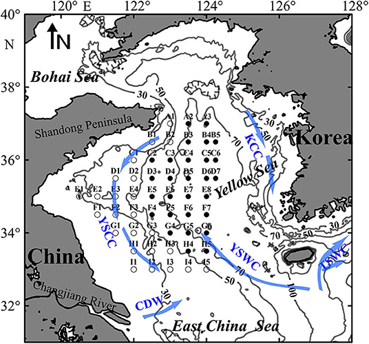
Figure 1. Map of the sampling stations in the Yellow Sea. Open and solid circles represent stations in the shallow and deep regions, respectively. Contour lines indicate water depth (m), and arrows represent circulation regimes, including Yellow Sea Warm Current (YSWC), Yellow Sea Coastal Current (YSCC), Korean Coastal Current (KCC), Changjiang Diluted Water (CDW), and Tsushima Warm Current (TSWC).

Zooplankton was vertically sampled using a Juday–Bogorov type net (diameter: 50 cm, mesh size: 160 μm) from the near bottom to the surface at each station. Confined by available ship-time, the sampling times were not fixed at day or night. The net was retrieved at a speed of ~1 m s⁻¹, and a calibrated flowmeter (Hydrobios) was used to measure the volume of filtered water. After collection, all samples were preserved in 5% neutral formalin seawater solution.

Vertical temperature and salinity profiles at each station were obtained by a Sea-Bird CTD instrument (SBE-19). Meanwhile, 500 mL seawater samples from each depth (0, 20, and 2–5 m from the bottom) were filtered onto a Whatman GF/F filter. The filters were extracted in 90% aqueous acetone for 24 h, then used to determine the content of chlorophyll a (Chl a) fluorometrically before and after acidification (Parsons et al., 1984).

In the laboratory, large zooplankton were firstly identified and counted. The remaining part was then subsampled until around 300–500 individuals were left in each subsample. All specimens in a subsample were identified to the species or the lowest taxonomic level and counted under a dissecting microscope. Zooplankton abundance (ind m⁻³) was calculated based on water volume filtered at each station. The abundance data of small copepods (SC), large copepods (LC), giant crustaceans (GC), and chaetognaths (CH) were transformed into dry weights (DW) according to length–dry weight relationships or references same as Sun et al. (2010). The dry weights of medusa (ME) and tunicates (TU) were not calculated due to their high water content.

Data Analysis

Multivariate analyses were performed using the PRIMER software V6.0 (Clarke and Gorley, 2006). Station clustering was performed for each survey dataset based on the Bray-Curtis similarity matrix of log (x+1) transformed zooplankton abundance and the average linkage group classification (Field et al., 1982). SIMPER (similarity percentages) analysis was used to assess the percent contributions of species to the similarity within groups and the dissimilarity between groups. ANOSIM (analysis of similarities) was used to test for the differences of zooplankton community structures between groups, with R-statistic value closer to 1 indicating greater difference.

The BIO-ENV procedure was used to evaluate the best sets of environmental factors (temperature, salinity, depth, Chl a) explaining the differences in zooplankton community structures. This process estimated the Spearman correlation coefficients (ρ) between the zooplankton and environmental factors similarity matrices, with ρ = 1 indicating a perfect match.

The zooplankton abundance, biomass, and environmental factors between groups were compared by one-way ANOVA using SPSS 19.0 software.

Results

Environmental Conditions

The distribution patterns of sea surface temperature (SST) and sea bottom temperature (SBT) were nearly consistent in winter, increasing southward and ranging from 7.5 to 13.0°C and from 7.9 to 12.8°C, respectively (Figure 2), as the water column was vertically well mixed (Figure 3). The SST also generally increased southward in the range of 11.8–20.2°C in spring, while the highest and lowest SBT occurred in the southwest and northwest coastal stations, respectively, ranging from 5.5 to 17.2°C (Figure 2). The SST ranges were 24.2–29.3°C and 18.5–21.0°C in summer and autumn, respectively. The Yellow Sea Cold Water Mass (YSCWM) begins to form in spring, well develops in summer, and decays in autumn. The YSCWM was located near the bottom of the central region of the Yellow Sea in summer and autumn, with <10°C SBT. However, the SBT did not exhibit the distribution pattern with lowest values in the deep area in spring, due to the presence of the Qingdao Cold Water Mass in the northwest coastal region (Figure 2). The highest SBT were 27.6 and 21.1°C in summer and autumn, respectively, and temperature fronts were found in the bottom layer at the edge of the YSCWM (Figure 2).

FIGURE 2

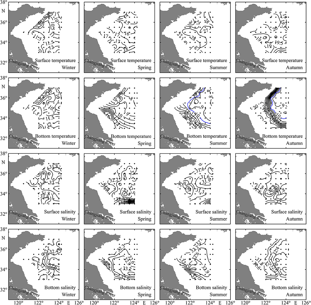
Figure 2. Spatial distributions of sea surface temperature (°C), bottom temperature (°C), surface salinity, and bottom salinity in the Yellow Sea during four seasons.

FIGURE 3

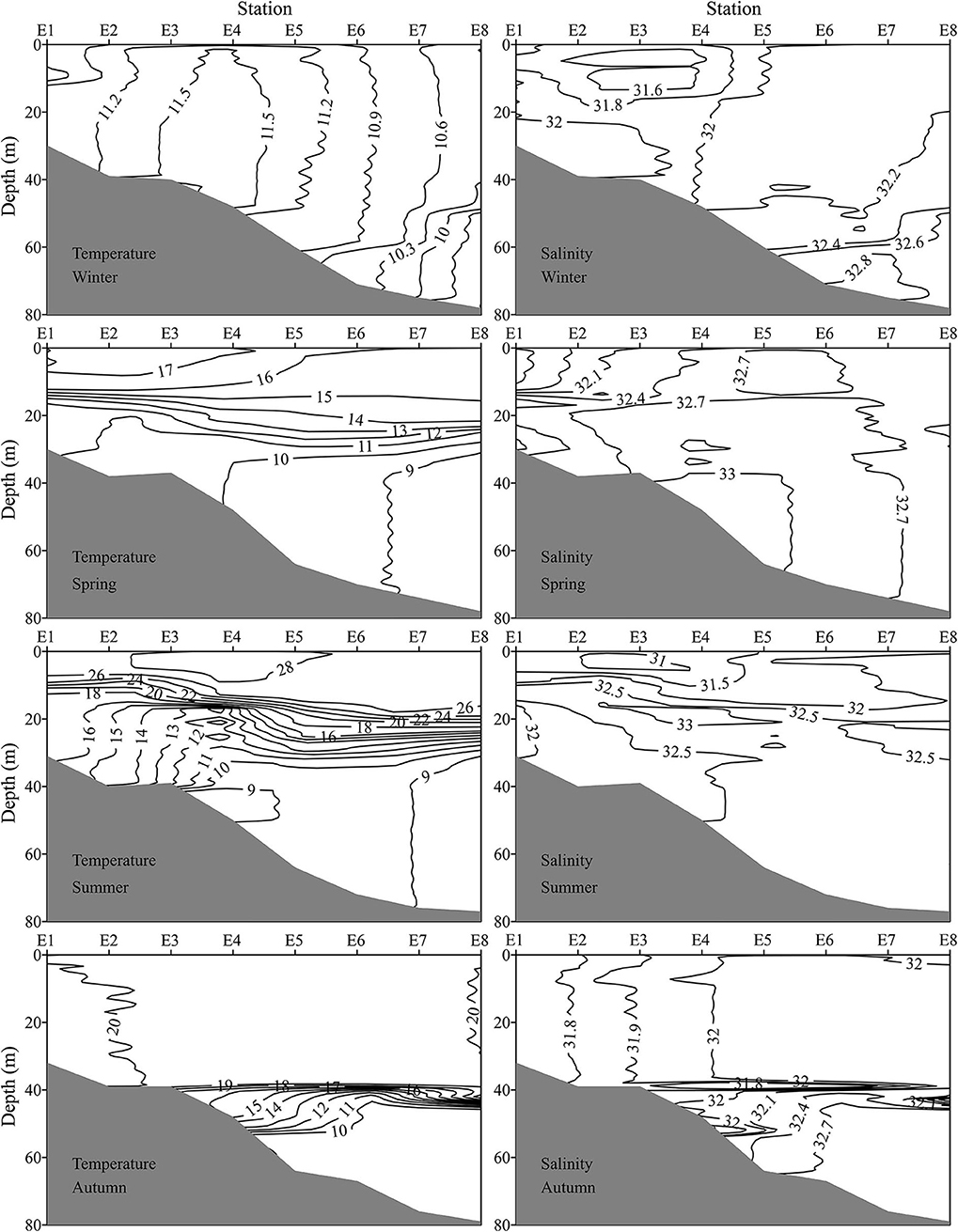
Figure 3. Vertical profiles of temperature (°C) and salinity along transect E (indicated in Figure 1) during four seasons.

The sea surface salinity (SSS) and sea bottom salinity (SBS) showed small differences in winter like temperature, and a water tongue with high salinity extended westward along the 34.5°N transect (Figure 2). The SSS had similar distribution patterns in spring and summer, with lowest values in the farthest south stations. Generally, coastal stations had relatively low SSS and SBS in all four seasons, and YSCWM region stations had high SBS from spring to autumn (Figure 2).

The E (35.0°N) transect passed through the YSCWM region and was selected to depict the vertical profile of temperature and salinity (Figure 3). No thermocline was found in winter. The thermocline started to develop between 15 and 30 m water depth in spring. The SST at all stations was higher than 26°C, and a strong thermocline existed in summer. The YSCWM with <10°C SBT was well developed at stations E4–E8 in summer. The mixed layer depth expanded to about 0–38 m, and the YSCWM shrunk to stations E5–E8 in autumn. Both SSS and SBS increased from E1 to E8. Generally, bottom layer in the YSCWM region had the highest salinity.

In general, the chlorophyll a concentrations at surface, 20 m depth, and bottom layers were all higher at coastal shallow stations than those at deep stations (Figure 4). The bottom Chl a was very low in the YSCWM stations in summer and autumn (Figure 4).

FIGURE 4

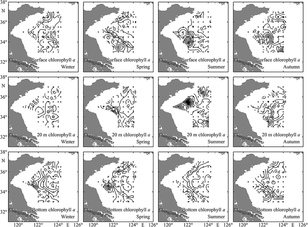
Figure 4. Spatial distributions of sea surface, 20 m depth, and bottom chlorophyll a concentrations (mg m⁻³) in the Yellow Sea during four seasons.

Stations in the shallow region had depth < 52 m, while the depth range in the deep region was 52–84 m (Figure 1 and Table 1). With the exception in summer, SST showed no significant differences (P > 0.05) between the shallow and deep regions in other three seasons. SBT was significantly lower (P < 0.01) in the deep region than in the shallow region from spring to autumn. SSS and SBS had significantly higher values (P < 0.05) in the deep region in all four seasons with the exception of SSS in autumn. Average water column chlorophyll a concentration was significantly higher (P < 0.01) in the shallow region in all four seasons (Table 1).

TABLE 1

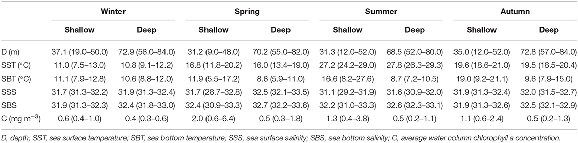
Table 1. Seasonal changes in environmental factors (mean and range) in the two domains in the Yellow Sea.

Zooplankton Community Structure

Seventy-three taxa (mostly at the species level) were identified in our study. A detailed abundance description of 27 taxa (> 90% total zooplankton abundance at any station) is presented in Table 2. Copepods clearly dominated the zooplankton community, and the dominant species were Oithona similis, Paracalanus sp., and Calanus sinicus.

TABLE 2

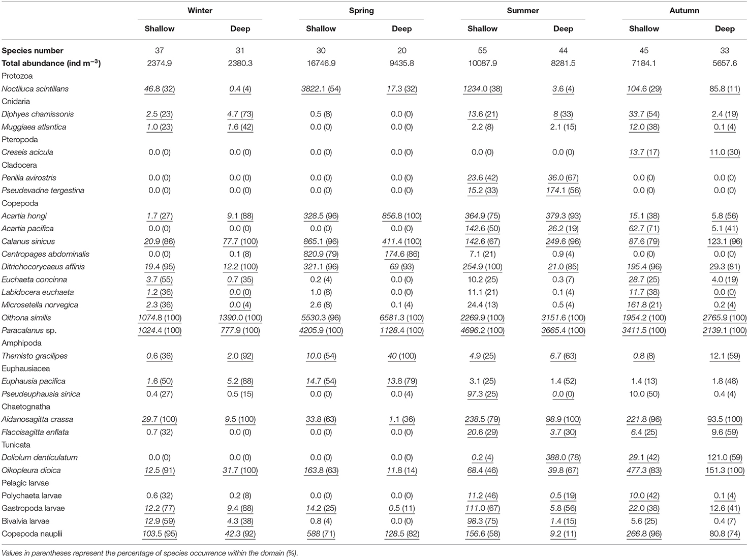
Table 2. Average abundances (ind m⁻³) of zooplankton species that contributed > 2% to community dissimilarities between domains (underlined numbers) and species number identified in the shallow and deep regions during four seasons in the Yellow Sea.

In all four seasons, zooplankton assemblage in the deep stations was separated from that in the coastal shallow stations based on cluster analysis of zooplankton abundance (Figure 5). The two domains, named shallow and deep regions, were divided by the 50 m isobath (Figures 1, 5).

FIGURE 5

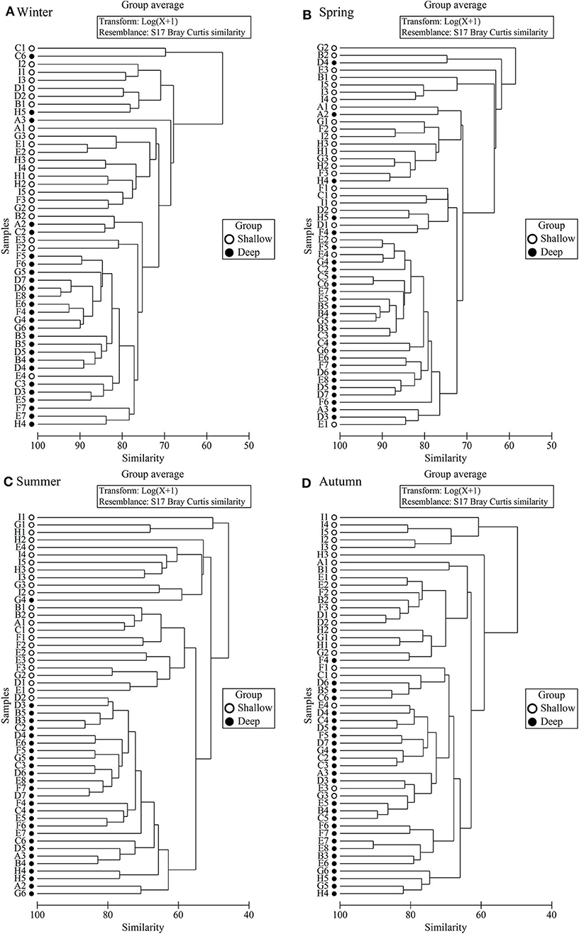
Figure 5. Dendrogram of station similarity based on cluster analysis of zooplankton abundance. (A) Winter, (B) Spring, (C) Summer, and (D) Autumn.

ANOSIM results showed that the zooplankton assemblages differed significantly (P < 0.001) between the shallow and deep regions in all four seasons (Table 3). SIMPER results indicated that the dissimilarity of zooplankton assemblages between the two domains was highest (47.3%) in summer and lowest (30.6%) in winter (Table 3). Zooplankton assemblage had higher similarities in the deep region than in the shallow region, and the similarities were highest in winter and lowest in summer in both domains (Table 3).

TABLE 3

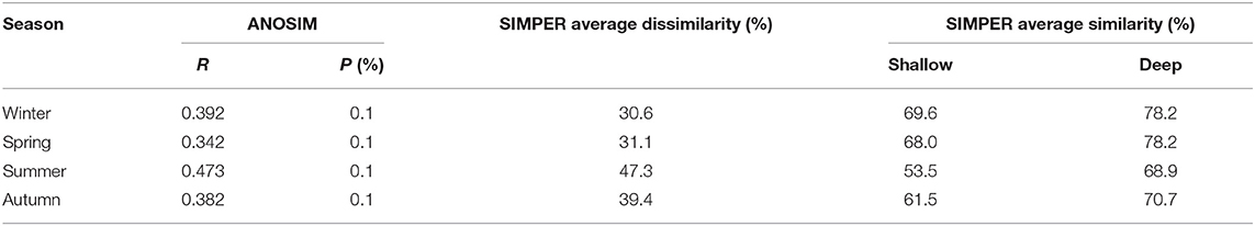
Table 3. Comparison of the zooplankton community structures between the shallow and deep regions in the Yellow Sea according to ANOSIM (R value and significance level) and SIMPER.

Seasonal Variation in Zooplankton Community

The mean total zooplankton abundance in the Yellow Sea was the highest in spring and followed a declining trend till winter (Table 2). Zooplankton in the shallow region usually had higher abundance and higher species number with the exception of abundance in winter (Table 2). The species number was 37 and 31 in the shallow and deep regions, respectively, in winter, while the numbers decreased to 30 and 20 in the two domains in spring. Species richness peaked in summer with 55 in the shallow region and 44 in the deep region. Then 45 and 33 zooplankton species were identified in autumn in the shallow and deep regions, respectively (Table 2).

In winter, based on the SIMPER analysis, C. sinicus, Copepoda nauplii, Acartia hongi, Bivalvia larvae, Oikopleura dioica, Gastropoda larvae, Euphausia pacifica, Aidanosagitta crassa, and Diphyes chamissonis all contributed > 5% to the zooplankton community dissimilarity between the shallow and deep regions. In spring, SIMPER results showed that Noctiluca scintillans, Copepoda nauplii, O. dioica, Centropages abdominalis, Themisto gracilipes, Ditrichocorycaeus affinis, A. crassa, and A. hongi contributed the most to the dissimilarity between domains. In summer, Doliolum denticulatum, Copepoda nauplii, Bivalvia larvae, C. sinicus, A. hongi, N. scintillans, and Pseudevadne tergestina were the main contributors to the community dissimilarity. In autumn, the main contributors to the dissimilarity were Copepoda nauplii, D. affinis, Acartia pacifica, D. denticulatum, O. dioica, C. sinicus, N. scintillans, and D. chamissonis (Table 2). Additionally, SIMPER results showed that O. similis, Paracalanus sp., C. sinicus and D. affinis all contributed > 4% to the zooplankton community similarity within any domain in any season.

Species with > 10% occurrence of total stations and accounting for > 1% of the total abundance of each main zooplankton taxa were defined as dominant species (Table 4). No significant differences were found in SC abundances between the shallow and deep regions in all four seasons (Figure 6A). Only in winter LC and GC abundances were significantly higher (P < 0.01) in the deep region than in the shallow region. CH abundance in the shallow region was significantly higher (P < 0.05) in all four seasons. ME in the shallow region had significantly higher abundance (P < 0.01) in autumn, while TU showed significant abundance differences (P < 0.05) between the two domains in winter, spring, and summer (Figure 6A).

TABLE 4

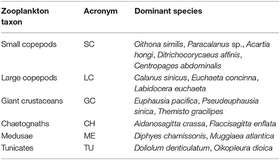
Table 4. Dominant species of six zooplankton taxa in the Yellow Sea.

FIGURE 6

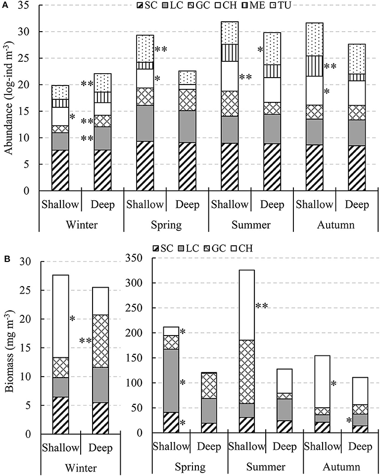
Figure 6. Seasonal changes in log-transformed abundance (A, log-ind m⁻³) and biomass (B, mg DW m⁻³) of zooplankton taxa in the two domains in the Yellow Sea. * and ** indicate significantly higher zooplankton taxa abundances or biomasses between domains in each season with P < 0.05 and P < 0.01, respectively.

The total biomass of the four zooplankton taxa (SC, LC, GC, and CH) was much lower in winter than that in other three seasons (Figure 6B). SC had higher biomass in the shallow region in all four seasons, with significant difference (P < 0.05) only in spring. LC had significantly higher biomass (P < 0.05) in the shallow region in spring and in the deep region in autumn. GC showed significant biomass difference (P < 0.01) between the two domains only in winter, with higher biomass in the deep region. CH biomass in the shallow region was significantly higher (P < 0.05) in all four seasons like abundance (Figure 6B).

GC biomass was usually higher in the deep stations, while CH usually had higher biomass in the shallow stations along the E transect (Figure 7). In spring, LC had high biomass in all the stations. LC and SC biomasses were much higher in station E7 in the YSCWM region in summer. The total biomass of SC, LC, and GC was relatively low in winter and autumn (Figure 7).

FIGURE 7

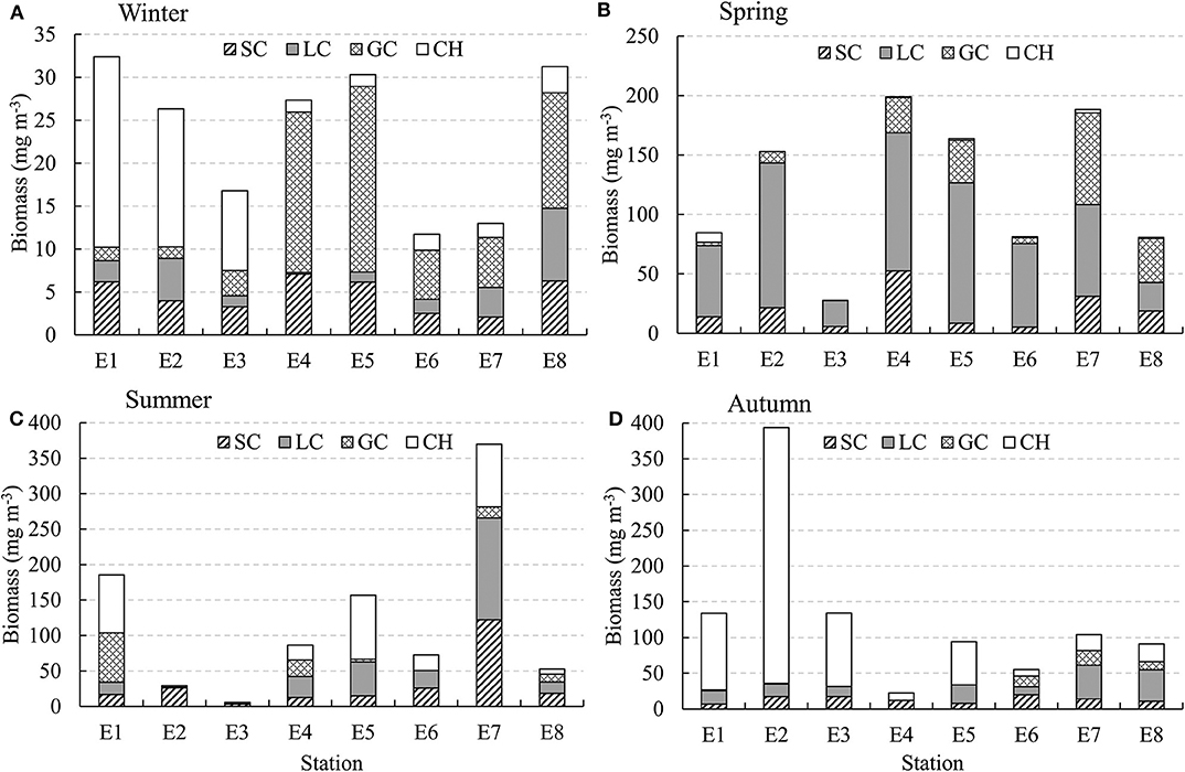
Figure 7. Seasonal changes in biomass (mg DW m⁻³) of zooplankton taxa along transect E (indicated in Figure 1) in the Yellow Sea. (A) Winter, (B) Spring, (C) Summer, and (D) Autumn.

Factors Affecting Community Structure

According to the BIO-ENV analysis (Table 5), a combination of depth, SST, and Chl a were the best environment variables to explain the variance in the community structure based on abundance in winter (ρ = 0.483). A combination of depth, SST, SBT, and SSS explained the most in spring (ρ = 0.516), while SBT was the best indicator in summer (ρ = 0.679), and depth and SBS were the best combination to indicate differences in the zooplankton community in autumn (ρ = 0.492) (Table 5).

TABLE 5

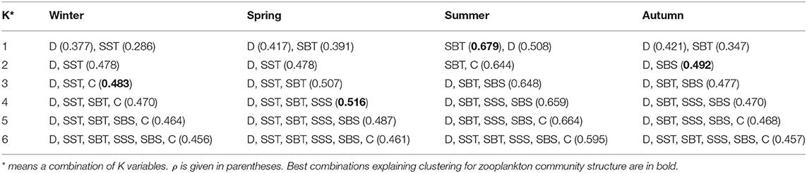
Table 5. BIO-ENV analysis of zooplankton community structure in the Yellow Sea during four seasons to depth (D), sea surface temperature (SST), sea bottom temperature (SBT), sea surface salinity (SSS), sea bottom salinity (SBS) and average water column chlorophyll a concentration (C).

Discussion

Community Structure and Distribution

Zooplankton species assemblages were associated with water mass distributions (Zuo et al., 2006; Domínguez et al., 2017). Based on the community structure, two distinct zooplankton assemblages, namely the Yellow Sea neritic and basin assemblages, spatially coincided with the shallow and deep regions of the study area (Zheng, 1965; Chen et al., 1980; Zuo et al., 2006). Zooplankton in the shallow region showed relatively low similarities (Table 3), due to the wide latitude range and seasonal variations in boundaries between zooplankton assemblages (Zheng, 1965; Chen et al., 2011). However, since two domains were separated by the 50 m isobath that demarcates ecologically important spawning-nursing and wintering grounds for many fishery species in the Yellow Sea, we assumed that the boundaries between two zooplankton assemblages were stable across four seasons.

Small copepods O. similis and Paracalanus sp. were the most abundant species in the present study with different distribution patterns. Oithona similis and A. hongi had higher abundances in the deep region (Table 2), which was consistent with previous observations in the Yellow Sea (Zuo et al., 2006; Shi et al., 2018); while the other small copepods, Paracalanus sp., D. affinis, C. abdominalis, A. pacifica, and Microsetella norvegica, were mostly distributed in the shallow region (Table 2). The comparable abundances between O. similis and Paracalanus sp. resulted in the small differences of SC abundances in the two domains. When transformed into dry weights, SC biomass was higher in the shallow region benefited from the higher DW of Paracalanus sp. (Figure 6).

Calanus sinicus dominated LC group, and most contributed to the LC abundance and biomass in the Yellow Sea (Sun et al., 2010; Huo et al., 2012). Higher LC biomass and C. sinicus abundance were found in the shallow region only in spring, confirming the C. sinicus life strategy that the population mainly propagated in the shallow region in spring, then moved toward the YSCWM region to survive through the hot summer (Sun, 2005).

The dominant species of GC were E. pacifica, T. gracilipes, and Pseudeuphausia sinica. Previous studies showed that high GC biomass was mainly located in the deep region in the Yellow Sea (Sun et al., 2010), as well as the E. pacifica and T. gracilipes populations (Wang and Zuo, 2004; Sun et al., 2011). Euphausia pacifica preferred to stay in the deep water (Wang and Zuo, 2004), making it seldom be sampled which might result in the low abundance in the present study. Compared with that higher abundance of T. gracilipes occurred in the deep region, E. pacifica did not show clear distribution preference from the view of abundance; however, both the two species exhibited much higher occurrence percentage in the deep region (Table 2). The high GC biomass in the shallow region in summer was contributed by the high P. sinica abundance.

Significantly higher CH abundance and biomass were found in the shallow region during all four seasons in the Yellow Sea, and ME had higher abundance in the shallow region from spring to autumn, suggesting their coastal distribution preference (Sun et al., 2012; Wang et al., 2013, 2016). TU dominant species D. denticulatum and O. dioica showed different distribution patterns, that D. denticulatum was distributed in the deep region while O. dioica was mainly located in the shallow region.

In the Japan Sea, a clear seasonal succession of zooplankton community structure occurred from dominance by cold-water copepods in winter–spring to prevalence of gelatinous and carnivorous plankton and small warm-water copepods in summer–autumn (Chiba and Saino, 2003). In the present study, the abundances of CH, ME, and tropical species Euchaeta concinna and D. denticulatum also increased in summer–autumn.

Environmental Factors Affecting Zooplankton Community

Depth was the most important single factor that affected the zooplankton community in the Yellow Sea (Table 5). Shallow water may enhance the mortality rate of zooplankton (Uye, 2000). Additionally, depth was the main contributor to the differences of environmental factors between the two domains in the present study. In the shallow region, the water column was relatively vertically well mixed due to tidal mixing (Liu et al., 2003), and an upwelling occurred in the frontal zone of the YSCWM in summer (Wei et al., 2016, 2018), both benefiting nutrient supply and phytoplankton reproduction. However, the more stratified conditions in the deep region in summer–autumn reduced nutrient concentrations at surface and maintained the cold and low Chl a YSCWM at bottom (Wei et al., 2016).

Temperature influenced the zooplankton community in two ways. Based on the view of seasonal succession, gelatinous plankton and warm-water species peaked in summer–autumn due to higher temperatures. Meanwhile, the YSCWM in the deep region provided a refuge for some low-temperature species, like C. sinicus and E. pacifica, to survive in summer (Sun, 2005; Sun et al., 2011). Higher abundances of low-saline species Labidocera euchaeta, A. pacifica, and Bivalvia larvae occurred in the shallow region suggesting the effect of salinity on the zooplankton distribution (Zuo et al., 2006; Shi et al., 2018). Rich nutrients and high Chl a in the shallow region benefited heterotrophic dinoflagellate N. scintillans population development (Glibert et al., 2018), where was also an ideal area for copepod recruitment (Sun, 2005; Shi et al., 2015), resulting in higher abundances of many small copepods and Copepoda nauplii during all four seasons as well as higher C. sinicus abundance in spring in the shallow region during the present study.

Water currents affected the zooplankton community by advective transport (Lü et al., 2013; Smeti et al., 2015; Peterson et al., 2017). The Yellow Sea Warm Current (YSWC), which is a prominent feature in winter in the Yellow Sea (Lin et al., 2011), brought tropical zooplankton species into the Yellow Sea and affected zooplankton biomass and migration patterns in the intrusion area (Wang and Zuo, 2004; Lü et al., 2013; Chen et al., 2020). Cladocerans P. tergestina and Penilia avirostris are low-saline species, with distribution associated with coastal water masses (Xu et al., 2007; Domínguez et al., 2017). High abundance of cladocerans that occurred in the deep region in summer in the present study suggested their transport by coastal current and river front.

Ecological Function of Zooplankton Taxa and Its Implications

The crustaceans SC, LC, and GC are the main food sources of many fish. As larval fish grow and the body length increases, the prey selectivity shifts from SC to LC, and then to GC (Meng, 2003). Importantly, small copepods are preferred prey during the critical fish larval stage due to their high abundance, appropriate size, and good nutritional value (Llopiz, 2013; Robert et al., 2014), affecting fish larvae survival and a subsequent recruitment to fish stocks (Hjort, 1914; Cushing, 1990).

The deep region of the Yellow Sea served as wintering grounds for many fishery species, while the shallow region is known to provide spawning, nursery, and foraging habitats (Jin et al., 2006; Xu and Chen, 2009). Higher abundances of LC and GC in the deep region in winter may support the wintering fish community, while higher SC and LC biomass and Copepoda nauplii abundance in the shallow region in spring could provide stable feeding grounds for larval fish. Additionally, the sampling net used in the present study (160 μm mesh) may have led to an underestimation of small copepods and copepod nauplii abundances (Atkinson et al., 2012; Chen et al., 2016).

Although SC biomass was relatively low when compared with LC and GC, SC had the highest production rate (Huo et al., 2012). Prey concentrations for maximum growth of larval marine fish range between 5 and 10 copepodites l⁻¹ (Munk, 1995; Peck and Daewel, 2007). In the present study, the abundance of small copepods in the shallow region satisfied the requirements of > 5 prey l⁻¹ for the larval fish survival from spring to autumn (Peck and Daewel, 2007). However, the high abundance of carnivorous CH and ME in summer–autumn may compete with larval fish for prey, and may directly feed on fish larvae. This study provides a foundation for future research to understand the inter-annual variability in seasonal development of plankton communities and main factors driving this variability.

Data Availability Statement

The datasets generated for this study are available on request to the corresponding author.

Author Contributions

JW, XS, and XJ contributed to the conception of the study. YS, JS, and WY contributed to sample collection and data collation. YS and TZ analyzed the samples and conducted the data analyses. YS and EP wrote the manuscript and contributed to the definition of aims. All authors contributed to the improvement of the manuscript before approving the submission.

Funding

This study was supported by the National Key R&D Program of China (2018YFD0900901), the Creative Team Project of QNLM LMEES (LMEES-CTSP-2018-4), the National Natural Science Foundation of China (31872692), the Central Public-interest Scientific Institution Basal Research Fund, YSFRI, CAFS (20603022020009), the Open Fund of QNLM LMEES (LMEES201807), Central Public-interest Scientific Institution Basal Research Fund, CAFS (2020TD01), and the China Scholarship Council (201803260001).

Conflict of Interest

The authors declare that the research was conducted in the absence of any commercial or financial relationships that could be construed as a potential conflict of interest.

Acknowledgments

We are grateful to the captain and crew of the R.V. Beidou for their efforts in the field and to colleagues who provided support during our sampling efforts. We are grateful to the University of British Columbia's Department of Earth, Ocean and Atmospheric Sciences for accommodating YS during his research visit.

References

Atkinson, A., Ward, P., Hunt, B. P. V., Pakhomov, E. A., and Hosie, G. W. (2012). An overview of Southern Ocean zooplankton data: abundance, biomass, feeding and functional relationships. CCAMLR Sci. 19, 171–218.

Google Scholar

Batchelder, H. P., Daly, K. L., Davis, C. S., Ji, R., Ohman, M. D., Peterson, W. T., et al. (2013). Climate impacts on zooplankton population dynamics in coastal marine ecosystems. Oceanography 26, 34–51. doi: 10.5670/oceanog.2013.74

CrossRef Full Text | Google Scholar

Beaugrand, G., Brander, K. M., Lindley, J. A., Souissi, S., and Reid, P. C. (2003). Plankton effect on cod recruitment in the North Sea. Nature 426, 661–664. doi: 10.1038/nature02164

PubMed Abstract | CrossRef Full Text | Google Scholar

Belkin, I. M. (2009). Rapid warming of Large Marine Ecosystems. Prog. Oceanogr. 81, 207–213. doi: 10.1016/j.pocean.2009.04.011

CrossRef Full Text | Google Scholar

Brun, P., Stamieszkin, K., Visser, A. W., Licandro, P., Payne, M. R., and Kiørboe, T. (2019). Climate change has altered zooplankton-fuelled carbon export in the North Atlantic. Nat. Ecol. Evol. 3, 416–423. doi: 10.1038/s41559-018-0780-3

PubMed Abstract | CrossRef Full Text | Google Scholar

Chen, H. J., Qi, Y. P., and Liu, G. X. (2011). Spatial and temporal variations of macro- and mesozooplankton community in the Huanghai Sea (Yellow Sea) and East China Sea in summer and winter. Acta Oceanol. Sin. 30, 84–95. doi: 10.1007/s13131-011-0108-5

CrossRef Full Text | Google Scholar

Chen, H. J., Yu, H., and Liu, G. X. (2016). Comparison of copepod collection efficiencies by three commonly used plankton nets: A case study in Bohai Sea, China. J. Ocean Univ. China 15, 1007–1013. doi: 10.1007/s11802-016-3122-6

CrossRef Full Text | Google Scholar

Chen, H. J., Zhu, Y. Z., and Liu, G. X. (2020). Characteristics of zooplankton community in North Yellow Sea unveiled an indicator species for the Yellow Sea Warm Current in winter: Euchaeta plana. J. Oceanol. Limnol. doi: 10.1007/s00343-019-9165-y. [Epub ahead of print].

CrossRef Full Text | Google Scholar

Chen, Q. C., Chen, Y. Q., and Hu, Y. Z. (1980). Preliminary study on the plankton communities in the southern Yellow Sea and the East China Sea [In Chinese, with English Abstract]. Acta Oceanol. Sin. 2, 149–157.

Google Scholar

Chiba, S., and Saino, T. (2003). Variation in mesozooplankton community structure in the Japan/East Sea (1991–1999) with possible influence of the ENSO scale climatic variability. Prog. Oceanogr. 57, 317–339. doi: 10.1016/S0079-6611(03)00104-6

CrossRef Full Text | Google Scholar

Clarke, K. R., and Gorley, R. N. (2006). PRIMER v6: User Manual/Tutorial. Plymouth: PRIMER-E.

Google Scholar

Cushing, D. (1990). Plankton production and year-class strength in fish populations: an update of the match/mismatch hypothesis. Adv. Mar. Biol. 26, 249–293. doi: 10.1016/S0065-2881(08)60202-3

CrossRef Full Text | Google Scholar

Domínguez, R., Garrido, S., Santos, A. M. P., and dos Santos, A. (2017). Spatial patterns of mesozooplankton communities in the Northwestern Iberian shelf during autumn shaped by key environmental factors. Estuar. Coast. Shelf Sci. 198, 257–268. doi: 10.1016/j.ecss.2017.09.008

CrossRef Full Text | Google Scholar

Dong, Z. J., Liu, D. Y., and Keesing, J. K. (2010). Jellyfish blooms in China: Dominant species, causes and consequences. Mar. Pollut. Bull. 60, 954–963. doi: 10.1016/j.marpolbul.2010.04.022

PubMed Abstract | CrossRef Full Text | Google Scholar

Field, J. G., Clarke, K. R., and Warwick, R. M. (1982). A practical strategy for analysing multispecies distribution patterns. Mar. Ecol. Prog. Ser. 8, 37–52. doi: 10.3354/meps008037

CrossRef Full Text | Google Scholar

Fu, M. Z., Wang, Z. L., Pu, X. M., Xu, Z. J., and Zhu, M. Y. (2012). Changes of nutrient concentrations and N:P:Si ratios and their possible impacts on the Huanghai Sea ecosystem. Acta Oceanol. Sin. 31, 101–112. doi: 10.1007/s13131-012-0224-x

CrossRef Full Text | Google Scholar

Glibert, P. M., Berdalet, E., Burford, M. A., Pitcher, G. C., and Zhou, M. J. (2018). Global Ecology and Oceanography of Harmful Algal Blooms. Ecological Studies 232. Springer. doi: 10.1007/978-3-319-70069-4

CrossRef Full Text | Google Scholar

Hays, G. C., Richardson, A. J., and Robinson, C. (2005). Climate change and marine plankton. Trends Ecol. Evol. 20, 337–344. doi: 10.1016/j.tree.2005.03.004

PubMed Abstract | CrossRef Full Text | Google Scholar

Hjort, J. (1914). Fluctuations in the great fisheries of northern Europe viewed in the light of biological research. Cons. Int. Explor. Mer. 20, 1–228.

Google Scholar

Huo, Y. Z., Sun, S., Zhang, F., Wang, M. X., Li, C. L., and Yang, B. (2012). Biomass and estimated production properties of size-fractionated zooplankton in the Yellow Sea, China. J. Mar. Syst. 94, 1–8. doi: 10.1016/j.jmarsys.2011.09.013

CrossRef Full Text | Google Scholar

Jin, X. S., Cheng, J. S., Qiu, S. Y., Li, P. J., Cui, Y., and Dong, J. (2006). Comprehensive Research and Evaluation of Fishery Resources in the Yellow Sea and Bohai Sea. Beijing: China Ocean Press (In Chinese).

Lin, C., Ning, X., Su, J., Lin, Y., and Xu, B. (2005). Environmental changes and the responses of the ecosystems of the Yellow Sea during 1976–2000. J. Mar. Syst. 55, 223–234. doi: 10.1016/j.jmarsys.2004.08.001

CrossRef Full Text | Google Scholar

Lin, X., Yang, J., Guo, Z., Zhang, Z., Yin, Y., Song, X., et al. (2011). An asymmetric upwind flow, Yellow Sea Warm Current: 1. New observations in the western Yellow Sea. J. Geophys. Res. 116, C04026. doi: 10.1029/2010JC006513

CrossRef Full Text | Google Scholar

Liu, G. M., Sun, S., Wang, H., Zhang, Y., Yang, B., and Ji, P. (2003). Abundance of Calanus sinicus across the tidal front in the Yellow Sea, China. Fish. Oceanogr. 12, 291–298. doi: 10.1046/j.1365-2419.2003.00253.x

CrossRef Full Text | Google Scholar

Llopiz, J. K. (2013). Latitudinal and taxonomic patterns in the feeding ecologies of fish larvae: a literature synthesis. J. Mar. Syst. 109–110, 69–77. doi: 10.1016/j.jmarsys.2012.05.002

CrossRef Full Text | Google Scholar

Lü, L. G., Wang, X., Wang, H. W., Li, L., and Yang, G. B. (2013). The variations of zooplankton biomass and their migration associated with the Yellow Sea Warm Current. Cont. Shelf Res. 64, 10–19. doi: 10.1016/j.csr.2013.05.007

CrossRef Full Text | Google Scholar

Meng, T. X. (2003). Studies on the feeding of anchovy (Engraulis japonicus) at different life stages on zooplankton in the Middle and Southern Waters of the Yellow Sea [In Chinese, with English Abstract]. Mar. Fish. Res. 24, 1–9.

Google Scholar

Mitra, A., Castellani, C., Gentleman, W. C., Jónasdóttir, S. H., Flynn, K. J., Bode, A., et al. (2014). Bridging the gap between marine biogeochemical and fisheries sciences; configuring the zooplankton link. Prog. Oceanogr. 129, 176–199. doi: 10.1016/j.pocean.2014.04.025

CrossRef Full Text | Google Scholar

Munk, P. (1995). Foraging behaviour of larval cod (Gadus morhua) influenced by prey density and hunger. Mar. Biol. 122, 205–212.

Google Scholar

Parsons, T. R., Maita, Y., and Lalli, C. M. (1984). A Manual of Chemical and Biological Methods for Seawater Analysis. Oxford: Pergamon Press.

Google Scholar

Peck, M. A., and Daewel, U. (2007). Physiologically based limits to food consumption, and individual-based modeling of foraging and growth of larval fishes. Mar. Ecol. Prog. Ser. 347, 171–183. doi: 10.3354/meps06976

CrossRef Full Text | Google Scholar

Peterson, W. T., Fisher, J. L., Strub, P. T., Du, X., Risien, C., Peterson, J., et al. (2017). The pelagic ecosystem in the Northern California Current off Oregon during the 2014–2016 warm anomalies within the context of the past 20 years. J. Geophys. Res. Oceans 122, 7267–7290. doi: 10.1002/2017JC012952

CrossRef Full Text | Google Scholar

Robert, D., Murphy, H. M., Jenkins, G. P., and Fortier, L. (2014). Poor taxonomical knowledge of larval fish prey preference is impeding our ability to assess the existence of a “critical period” driving year-class strength. ICES J. Mar. Sci. 71, 2042–2052. doi: 10.1093/icesjms/fst198

CrossRef Full Text | Google Scholar

Shi, Y. Q., Sun, S., Li, C. L., and Zhang, G. T. (2016). Interannual changes in the abundance of zooplankton functional groups in the southern Yellow Sea in early summer [In Chinese, with English Abstract]. Oceanol. Limnol. Sin. 47, 1–8.

Shi, Y. Q., Sun, S., Zhang, G. T., Wang, S. W., and Li, C. L. (2015). Distribution pattern of zooplankton functional groups in the Yellow Sea in June: a possible cause for geographical separation of giant jellyfish species. Hydrobiologia 754, 43–58. doi: 10.1007/s10750-014-2070-7

CrossRef Full Text

Shi, Y. Q., Zuo, T., Yuan, W., Sun, J. Q., and Wang, J. (2018). Spatial variation in zooplankton communities in relation to key environmental factors in the Yellow Sea and East China Sea during winter. Cont. Shelf Res. 170, 33–41. doi: 10.1016/j.csr.2018.10.004

CrossRef Full Text | Google Scholar

Smeti, H., Pagano, M., Menkes, C., Lebourges-Dhaussy, A., Hunt, B. P. V., Allain, V., et al. (2015). Spatial and temporal variability of zooplankton off New Caledonia (Southwestern Pacific) from acoustics and net measurements. J. Geophys. Res. Oceans 120, 2676–2700. doi: 10.1002/2014JC010441

CrossRef Full Text | Google Scholar

Steinberg, D. K., and Landry, M. R. (2017). Zooplankton and the ocean carbon cycle. Annu. Rev. Mar. Sci. 9, 413–444. doi: 10.1146/annurev-marine-010814-015924

PubMed Abstract | CrossRef Full Text | Google Scholar

Sun, S. (2005). Over-summering strategy of Calanus sinicus. GLOBEC Int. Newsl. 11, 34.

Google Scholar

Sun, S. (2016). Fishery Version 3.0. [In Chinese, with English Abstract]. Bull. Chin. Acad. Sci. 31, 1332–1338. doi: 10.16418/j.issn.1000-3045.2016.12.007

CrossRef Full Text

Sun, S., Huo, Y. Z., and Yang, B. (2010). Zooplankton functional groups on the continental shelf of the yellow sea. Deep Sea Rea. II 57, 1006–1016. doi: 10.1016/j.dsr2.2010.02.002

CrossRef Full Text | Google Scholar

Sun, S., Tao, Z. C., Li, C. L., and Liu, H. L. (2011). Spatial distribution and population structure of Euphausia pacifica in the Yellow Sea (2006–2007). J. Plankton Res. 33, 873–889. doi: 10.1093/plankt/fbq160

CrossRef Full Text | Google Scholar

Sun, S., Zhang, F., Li, C. L., Yang, B., and Ji, P. (2012). The distribution pattern of small medusae in the Yellow Sea [In Chinese, with English Abstract]. Oceanol. Limnol. Sin. 43, 429–437.

Google Scholar

Tang, Q. S. (2009). “Changing states of the Yellow Sea Large Marine Ecosystem: anthropogenic forcing and climate impacts,” in Sustaining the World's Large Marine Ecosystems, eds K. Sherman, M.C. Aquarone, and S. Adams (Gland: IUCN), 77–88.

Google Scholar

Tang, Q. S., Ying, Y. P., and Wu, Q. (2016). The biomass yields and management challenges for the Yellow sea large marine ecosystem. Environ. Dev. 17, 175–181. doi: 10.1016/j.envdev.2015.06.012

CrossRef Full Text | Google Scholar

Turner, J. T. (2004). The importance of small planktonic copepods and their roles in pelagic marine food webs. Zool. Stud. 43, 255–266.

Google Scholar

Uye, S. I. (2000). Why does Calanus sinicus prosper in the shelf ecosystem of the Northwest Pacific Ocean? ICES J. Mar. Sci. 57, 1850–1855. doi: 10.1006/jmsc.2000.0965

CrossRef Full Text | Google Scholar

Wang, R., and Zuo, T. (2004). The Yellow Sea Warm Current and the Yellow Sea Cold Bottom Water, their impact on the distribution of zooplankton in the southern Yellow Sea. J. Korean Soc. Oceanogr. 39, 1–13.

Google Scholar

Wang, X., Jiang, M. J., Liu, P., Zhang, X. L., Wang, Y., and Wang, Z. L. (2016). Distribution pattern of zooplankton and its influencing factors in the South Yellow Sea in autumn [In Chinese, with English Abstract]. Haiyang Xuebao 38, 125–134. doi: 10.3969/j.issn.0253-4193.2016.10.013

CrossRef Full Text

Wang, X., Wang, Z. L., Pu, X. M., and Liu, P. (2013). Analysis of the distribution of zooplankton in the Southern Yellow Sea in summer and its influencing factors [In Chinese, with English Abstract]. Acta Oceanol. Sin. 35, 147–155. doi: 10.3969/j.issn.0253-4193.2013.05.016

CrossRef Full Text

Wei, Q. S., Li, X. S., Wang, B. D., Fu, M. Z., Ge, R. F., and Yu, Z. G. (2016). Seasonally chemical hydrology and ecological responses in frontal zone of the central southern Yellow Sea. J. Sea Res. 112, 1–12. doi: 10.1016/j.seares.2016.02.004

CrossRef Full Text | Google Scholar

Wei, Q. S., Wang, B. D., Yao, Q. Z., Fu, M. Z., Sun, J. C., Xu, B. C., et al. (2018). Hydro-biogeochemical processes and their implications for Ulva prolifera blooms and expansion in the world's largest green tide occurrence region (Yellow Sea, China). Sci. Total Environ. 645, 257–266. doi: 10.1016/j.scitotenv.2018.07.067

PubMed Abstract | CrossRef Full Text | Google Scholar

Xu, Z. L., and Chen, J. J. (2009). Analysis on migratory routine of Larimichthy polyactis [In Chinese, with English Abstract]. J. Fish. Sci. China 16, 931–940. doi: 10.3321/j.issn:1005-8737.2009.06.014

CrossRef Full Text | Google Scholar

Xu, Z. L., Gao, Q., Chen, H., Chen, J. J., and Cai, M. (2007). Ecological adaptation of pelagic Cladocera and Cumacea in East China Sea [In Chinese, with English Abstract]. Chin. J. Ecol. 26, 1782–1787. doi: 10.13292/j.1000-4890.2007.0319

CrossRef Full Text | Google Scholar

Yang, Y., Sun, X. X., Zheng, S., and Zhao, Y. F. (2016). Distribution and long-term variation of net phytoplankton in south Yellow Sea in early summer [In Chinese, with English Abstract]. Oceanol. Limnol. Sin. 47, 755–763. doi: 10.11693/hyhz20160200028

CrossRef Full Text

Yu, R. C., and Liu, D. Y. (2016). Harmful algal blooms in the coastal waters of China: current situation, long-term changes and prevention strategies [In Chinese, with English Abstract]. Bull. Chin. Acad. Sci. 31, 1167–1174. doi: 10.16418/j.issn.1000-3045.2016.10.005

CrossRef Full Text

Zhang, B., Tang, Q. S., and Jin, X. S. (2007). Decadal-scale variations of trophic levels at high trophic levels in the Yellow Sea and the Bohai Sea ecosystem. J. Mar. Syst. 67, 304–311. doi: 10.1016/j.jmarsys.2006.04.015

CrossRef Full Text | Google Scholar

Zhao, X. Y., Hamre, J., Li, F. G., Jin, X. S., and Tang, Q. S. (2003). Recruitment, sustainable yield and possible ecological consequences of the sharp decline of the anchovy (Engraulis japonicus) stock in the Yellow Sea in the 1990s. Fish. Oceanogr. 12, 495–501. doi: 10.1046/j.1365-2419.2003.00262.x

CrossRef Full Text | Google Scholar

Zheng, Z. Z. (1965). The structure of zooplankton communities and its seasonal variation in the Yellow Sea and in the western East China Sea [In Chinese, with English Abstract]. Oceanol. Limnol. Sin. 7, 199–204.

Google Scholar

Zuo, T., Wang, R., Chen, Y. Q., Gao, S. W., and Wang, K. (2006). Autumn net copepod abundance and assemblages in relation to water masses on the continental shelf of the Yellow Sea and East China Sea. J. Mar. Syst. 59, 159–172. doi: 10.1016/j.jmarsys.2005.09.008

CrossRef Full Text | Google Scholar