Material Residence Time in Marine Canopies Under Wave-Driven Flows

Coastal canopies (e.g., seagrasses, coral reefs, and kelp forests) are vitally important ecosystems that provide a range of ecological services (e.g., oxygen production, sediment stabilization and trapping, and recycling of nutrients). The long-term health, productivity, and survival of these canopies rely heavily on the residence time of ecologically-significant materials in these environments. Recent studies have shown that submerged canopies induce a strong mean current over the canopy top, even in purely wave-dominated environments. Thus, in addition to vertical mixing, the horizontal flushing of materials (resulting from these canopy-induced currents) will dictate rates of water renewal and, therefore, residence time in wave-dominated flows over submerged canopies. Building on this recently-improved understanding, this paper provides (for the first time) a framework for estimation of material residence time (T_res) and its variation with core system parameters, including both canopy and wave characteristics. This is done through consideration of a Péclet number (Pe) which is the ratio of mixing to advective time scales. Prediction of residence time for a wide and realistic range of marine canopies (and a correspondingly wide range of Pe) reveals that while T_res decreases with wave height and increases with water depth, it has a complex relationship with canopy density and height. Importantly, residence time can vary from orders of seconds to hours, depending on wave and canopy properties. This has considerable ecological implications for marine canopies through the direct impact on a range of chemical and biogeochemical processes within the canopy. The framework presented here represents a critical step forward in being able to predict residence time in coastal canopies and test the interacting set of factors that influence the residence time in real, complex systems.

1. Introduction

Coastal canopies, such as those formed by seagrass meadows, coral communities, and kelp forests (Duarte, 2002; Rosman et al., 2007), provide food (Connolly et al., 2005), nursery, habitat (Fonseca et al., 1992), and shelter (Scott et al., 2000) for a wide range of marine organisms (Gambi et al., 1990; Koch et al., 2006). These canopies influence water quality through the direct uptake of nutrients (Moore, 2004; Larkum et al., 2006), particulate materials (Gacia et al., 2002), as well as the production of oxygen (Larkum et al., 2006). The drag exerted by aquatic canopies has a significant impact on the local hydrodynamics by reducing the in-canopy velocity (Lowe et al., 2005; Abdolahpour et al., 2017a) and dissipating wave energy (Kobayashi et al., 1993), which in turn leads to enhanced sedimentation (Gacia et al., 1999), carbon burial (Granata et al., 2001), and retention of particulate material within the meadow (Fonseca and Cahalan, 1992).

Most of these ecological functions are tightly limited by the exchange of water across canopy boundaries and, more specifically, the canopy residence time (T_res). An accurate quantification of residence time (i.e., the time scale over which water parcels are retained within the canopy) is critical as it improves our ability to predict the availability of materials to react with biologically or geochemically active surfaces; for example, the timescale over which a pulse of nutrients is available for uptake by seagrass leaves. Residence time, and the specific hydrodynamic processes that control it, can have significant effects on pollen and seed dispersal (Orth et al., 1994; Ackerman, 2002) and sediment deposition (Gacia et al., 1999). The in-canopy hydrodynamics (Helmuth and Sebens, 1993) and turbulence structure (Sebens et al., 1997) have also been shown to have a tremendous effect on many biological processes within the canopy. For example, the velocity reduction within canopies results in a significant increase in the rate of filter-feeding (Brun et al., 2009), particle capture (Helmuth and Sebens, 1993; Sebens et al., 1997), and nutrient uptake in coastal environments (Thomas and Cornelisen, 2003; Weitzman et al., 2013). In addition to the implications for macrophytes that take up nutrients from the water column, residence time can play an important role for biogeochemical cycling within the hyporheic zone, one of the most significant regions for material storage (Harvey et al., 2003; Zarnetske et al., 2011).

Very few studies have looked at the residence time of solutes (Worcester, 1995; Harvey et al., 2005; Lara et al., 2012) and particulate materials (Ackerman, 2002; Defina and Peruzzo, 2012) within aquatic canopies, the majority of which focused on current-dominated environments. However, many aquatic canopies are located in coastal environments and are exposed to shallow water waves. The oscillatory nature of wave-dominated flows profoundly influences the hydrodynamics and turbulent diffusion in these environments (Reidenbach et al., 2007; Abdolahpour et al., 2017a,b). For example, the in-canopy velocity (relative to the above-canopy velocity) is significantly enhanced under oscillatory flow conditions compared to the corresponding unidirectional flow (Lowe et al., 2005) while turbulent mixing substantially decreases in wave-dominated environments (Abdolahpour et al., 2017a). The competing effects of in-canopy velocity reduction and enhanced turbulent mixing can greatly alter the residence time of ecologically-important materials in these environments (e.g., Thomas and Cornelisen, 2003; Falter et al., 2004). Thus, a specific assessment of residence time in wave-dominated canopy flows is necessary. This research aims to fill this gap by developing a framework under which a predictive estimation of residence time across a wide range of field conditions will be available.

2. Model Development

In coastal ecosystems (where the flow is typically wave-dominated), there are two important mechanisms dictating flux across canopy boundaries; namely, (a) vertical mixing (Abdolahpour et al., 2017a) and (b) horizontal advection (Luhar et al., 2010; Abdolahpour et al., 2017b). This time-averaged horizontal advection is generated by the roughness of the canopy, even though the ambient flow is purely wave-driven. Both processes are complex functions of the canopy and flow properties and can have tremendous impacts on transport (and therefore, residence time) of nutrients (Morris et al., 2008), pollen (Ackerman, 2002), seeds (Orth et al., 1994), and sediment (Gacia et al., 1999). Here, we aim to develop a physically-based framework that incorporates our understanding of these two important flushing mechanisms to predict residence times in coastal (and therefore, wave-dominated) canopies.

2.1. Vertical Mixing in Coastal Canopies

In coastal canopies, the drag exerted by the canopy elements results in a vertical gradient of orbital velocity across the canopy-water interface (Lowe et al., 2005; Pujol et al., 2013; Abdolahpour et al., 2017a). That is, the velocity within the canopy, $U_c^{rms}$ (with the superscript “rms” referring to the root-mean-square of the orbital velocity and the subscript “c” to the in-canopy average hereafter), is attenuated from its value far above the canopy, $U_{\infty }^{rms}$ (Figure 1A). The difference between the above- and within-canopy RMS velocities is denoted as ΔU. This velocity attenuation, which increases with canopy density (Lowe et al., 2005; Abdolahpour et al., 2017a), creates an inflectional shear layer in the vertical profile of oscillatory velocity. This can lead to the generation of Kelvin-Helmholtz (KH) vortices across the top of the canopy (Figure 1A) (Ghisalberti and Schlosser, 2013). These vortices can significantly enhance the rate of vertical exchange of dissolved and particulate material, as seen in current-dominated environments (Ghisalberti and Nepf, 2005).

FIGURE 1

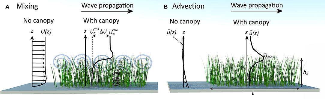
Figure 1. Interactive effects of wave-dominated flows over submerged canopies. (A) The strong velocity gradient at the canopy top causes the generation of large scale KH-vortices in this region (gray spirals). These vortices, together with wake turbulence (small circles inside the canopy), control rates of vertical mixing in coastal canopies. (B) The asymmetry in particle motion (resulted from the canopy drag) causes the generation of a strong mean drift ($\overline{u}$) within a confined region above the canopy (Abdolahpour et al., 2017b). Note, h_c and L indicate the height and length of a typical canopy, respectively.

While these shear-driven vortices dominate vertical exchange in steady flows, mixing in coastal canopies is dictated by a coupled contribution of both shear- and wake-driven mixing (Abdolahpour et al., 2017a). The vertical diffusivity in rigid canopies (such as hard corals) is given by:

$\begin{array}{ll}{D}_{t,z}=0.04\Delta U{L}_D+0.58\sqrt[3]{\frac{d}{L_D}}{U}_c^{rms}d& (1)\end{array}$

In this equation, D_{t, z} is the vertical turbulent diffusivity, d is the stem diameter and L_D is the drag length scale, defined as:

$\begin{array}{ll}{L}_D=\frac{1-{\lambda }_P}{C_{D}a}& (2)\end{array}$

with λ_p being the solid fraction of the canopy, a the canopy frontal area per unit volume canopy and C_D ≈ 1 the drag coefficient (after Abdolahpour et al., 2017a). The first term on the right hand side of Equation (1) represents the contribution of shear-driven mixing and the second term the contribution of wake-driven mixing. As seen, the extent of the contribution of each process varies with wave and canopy properties, highlighting the complexity of residence time prediction in these environments.

Our recently-improved understanding reveals that canopy flexibility can have a significant impact on flow, turbulence and, ultimately, rates of vertical mixing. In particular, rates of vertical mixing has been shown to be always less in flexible canopies compared to corresponding rigid canopies (by 35%, on average). Thus, a correction factor of 0.65 must be applied for an accurate estimation of vertical mixing in flexible canopies such as seagrasses (Abdolahpour et al., 2018). Thus, the vertical diffusivity in these environments can be given by:

$\begin{array}{ll}{D}_{t,z}=0.028\Delta U{L}_D+0.38\sqrt[3]{\frac{b}{L_D}}{U}_c^{rms}b& (3)\end{array}$

with b being the blade width.

While shear layer vortices are a ubiquitous feature (and control vertical mixing) in current-dominated canopy flows, they are only generated in wave-dominated flows when particular wave and canopy conditions are met (see Ghisalberti and Schlosser, 2013). However, the predictive models in Equations (1) and (3) consider both shear-layer and wake mixing and have been tested for conditions in which vortices are both present and absent. Thus, both formulations can conveniently be used for estimating rates of vertical mixing in a wide range of field conditions.

2.2. Horizontal Advection in Coastal Canopies

In the presence of a canopy, the vertical velocity gradients across the top of submerged coastal canopies (see the typical velocity profile in Figure 1A) drive an asymmetry in particle motion over the wave cycle. This causes fluid particles (located adjacent to the canopy top) to move faster in the shoreward direction above the canopy under a crest than in the seaward direction within the canopy under a trough, leading to the generation of a mean current in the direction of wave propagation ($\overline{u}$) (Abdolahpour et al., 2017b) (Figure 1B). The maximum current magnitude (${\overline{u}}_{max}$) occurs at the top of the canopy, and is observed to be up to 75% of the above-canopy orbital velocity (Abdolahpour et al., 2017b). The magnitude of this current depends on the characteristic velocity far above the canopy ($U_{\infty }^{rms}$) and the canopy drag length scale (L_D) according to:

$\begin{array}{ll}{\overline{u}}_{max}=0.5U_{\infty }^{rms}{\left(\frac{{\xi }_T}{L_D}\right)}^{0.3}& (4)\end{array}$

where ξ_T is the vertical particle excursion at the canopy top (Abdolahpour et al., 2017b). In practice, it is more common, and convenient, to measure wave height rather than ξ_T; the two are related simply according to linear wave theory:

$\begin{array}{ll}{\xi }_T=H\frac{sinh(k{h}_c)}{sinh(kh)}& (5)\end{array}$

where H is the wave height, h_c the canopy height, h the water depth and k is the wave number (Dean and Dalrymple, 1991). As can be inferred from Equation (4), the magnitude of the current increases with wave velocity and canopy density (i.e., decreasing L_D). This shoreward drift, which has been observed both in the laboratory (Lowe et al., 2005; Luhar et al., 2010; Abdolahpour et al., 2017b) and field (Luhar et al., 2013), can have a significant impact on material exchange by introducing a second method of water renewal through horizontal flushing of dissolved and particulate material. Thus, although coastal systems are typically wave-dominated (Koch et al., 2006), the impact of canopy-induced currents on residence time may not be negligible.

While Equation (4) has been developed using linear wave theory (for simplicity), its applicability has been tested and validated over a wide range of experimental and field conditions (including shallow, intermediate and deep water waves, as well as in both rigid and flexible canopies) (Abdolahpour, 2017). This model is also in excellent agreement with numerical simulations (van Rooijen et al., 2020). Thus, we expect the advection model to be valid in a variety of submerged canopies exposed to a wide range of water waves (in the absence of ambient mean currents).

In coastal canopies exposed to purely wave-driven flows, the residence time will depend on two important time scales; namely T_mix and T_adv which are the diffusive and advective time scales, respectively, and can be expressed as:

$\begin{array}{ll}{T}_{mix}=\frac{{h_c}^2}{D_{t,z}}& (6)\end{array}$

and

$\begin{array}{ll}{T}_{adv}=\frac{L}{{\overline{u}}_{max}}& (7)\end{array}$

with L being the canopy length (Figure 1B).

Note, both mixing (Equations 1 or 3) and advection (Equation 4) formulations are generalized in terms of the canopy drag length scale (e.g., L_D), instead of species-specific characteristics. Thus, they are relevant and applicable across all canopies (e.g., seagrass, coral, kelp), as long as the key canopy and wave characteristics are known.

2.3. Theoretical Framework

The relative importance of vertical mixing and horizontal flushing (due to the roughness-generated mean current), i.e., the Péclet number (Pe), can conveniently be used as a tool to identify the dominant time scale that dictates residence time in wave-dominated canopy flows. Here, the Péclet number is defined as:

$\begin{array}{ll}Pe=\frac{T_{mix}}{T_{adv}}& (8)\end{array}$

Through substitution of (6) and (7) into (8), the canopy Péclet number can be expressed as:

$\begin{array}{ll}Pe=\frac{{\overline{u}}_{max}{h_c}^2}{L{D}_{t,z}}& (9)\end{array}$

When Pe ≪ 1, residence time (T_res) is dominantly controlled by vertical mixing and can be evaluated through Equation (6) and the predictive formulation for D_{t, z} (i.e., Equation 1 or 3). Conversely, when Pe≫1, residence time is controlled by advection and can be evaluated through Equation (7) and the predictive formulation for ${\overline{u}}_{max}$ (i.e., Equation 4). When Pe ~ O(1), both advection and diffusion will influence the residence time of dissolved and particulate materials in aquatic canopies. The ecological and environmental implication of this classification is significant. When transport is mixing-dominated (i.e., Pe ≪ 1), water renewal is expected to occur mainly through vertical replenishment across the canopy-water interface. Thus, it is expected that supply of nutrients, oxygen, pollen, spores, suspended sediments, and contaminants will be limited to the overlaying water. As an example, in pollen dispersal dynamics, this may increase the probability of local pollination success and reduce the chance of dispersal over longer distance due to more limited horizontal movement of pollen. In contrast, when the flow is advection-dominated (i.e., Pe≫1), water renewal will primarily be controlled by horizontal flushing and the likelihood of material exchange to and from the overlying water decreases. Finally, when both processes are significant [i.e., Pe ~ O(1)], advection and diffusion are of the same orders of magnitude and either T_mix or T_adv can be used as an approximate estimation of residence time. This is further demonstrated in the following sections through characterization of the Péclet number and, ultimately, residence time in typical marine canopies.

2.4. The Variation of the Péclet Number in Coastal Canopies

Both vertical mixing and horizontal flushing are heavily dependent on wave and canopy conditions, properties that vary widely between sites, seasons, and species. Typically, marine canopies exist in coastal regions and are exposed to shallow water waves. This is mainly due to the light availability in these regions. Some seagrass species, kelps, and many coral communities, however, can be found in deeper regions and may be exposed to transitional or deep water waves (Larkum et al., 2006). This results in a wide range of wave conditions that canopies are exposed to in the real system. For example, marine canopies may exist under swell waves with wave period T ~ O(1−10 s), H ~ O(10−100 cm), and water depth h ~ O(1−10 m) (Infantes et al., 2009; Mohring and Rule, 2014) (see Table 1) which could include shallow, intermediate or deep water waves. Additionally, the drag length scale of typical marine canopies is O(1−100 cm) and the canopy length is O(1−100 m) (Cambridge and Kuo, 1979; Kendrick et al., 2005; Oreska et al., 2017). As an example, Figure 2 shows the variability of canopy height and density; in these cases, induced by differences in light availability in a meadow of P. sinuosa seagrass, in Jurien Bay, Western Australia. The canopy length was approximately 50 m, and values of height and dimensionless frontal areas for each case (data from Collier et al., 2009) are shown on the figure. Clearly, meadows located in sites with heavy shading are sparser and shorter than those exposed to clear water with high ambient light. This variability in canopy density and height is a great indicator of how light reduction from other processes (e.g., high levels of suspended sediment concentration) would impact canopy properties, and ultimately, the residence time in these environments. This is indicative of variability both within individual canopies (over time) and across different canopies.

TABLE 1

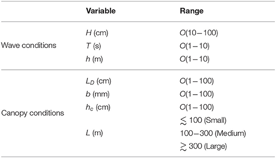
Table 1. Typical wave and canopy conditions in coastal systems (Cambridge and Kuo, 1979; Kendrick et al., 2005; Infantes et al., 2009; Mohring and Rule, 2014; Oreska et al., 2017).

FIGURE 2

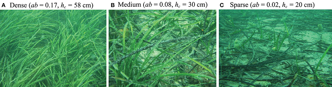
Figure 2. Pictures showing varying canopy density due to imposed light level in meadows of Posidonia sinuosa seagrass, located at Jurien Bay, Western Australia. Increasing shading (from A–C) reduced canopy density and height (data and pictures from Collier et al., 2009).

Due to the significant spatial and temporal variation in time scales of vertical mixing and horizontal flushing, the value of Pe for marine canopies is expected to be highly variable. To demonstrate this, Figure 3 depicts how Pe (defined in Equation 9) may vary in a typical canopy exposed to coastal waves. While the model developed here is relevant for a range of coastal canopies (e.g., coral reefs, seagrass meadows, and kelp forests), we chose typical characteristics of P. australis as an example to perform analysis and to illustrate the major variations. A wave period of T = 10 s (typical of marine ecosystems) and blade width of b = 1 cm are employed for all calculations hereafter. The in-canopy velocities were estimated using the theoretical model proposed by Lowe et al. (2005). This model provides an estimate of the velocity ratio, α ($=U_c^{rms}/U_{\infty }^{rms}$), such that knowledge of $U_{\infty }^{rms}$ and canopy properties (i.e., L_D) leads to the estimation of ΔU ($=U_{\infty }^{rms}-\alpha U_{\infty }^{rms}$). Thus, this model can conveniently be used to predict the in-canopy velocity where the typical wave and canopy properties are known. As seen, the Péclet number varies significantly, depending on wave and canopy properties (Figure 3). For instance, the canopy height alone can have a substantial impact on Pe, such that changes in h_c due to, e.g., seasonal (Collier et al., 2007), depth (Bulthuis and Woelkerling, 1983), and light (Collier et al., 2009) variation may cause a particular canopy to be in the mixing-dominated regime in one season (or location) and in advection-dominated environment in another. This is further illustrated by calculating values of the Péclet number for canopies shown in Figures 2A–C (black markers in Figure 3). While the flow is mixing-dominated when the canopy is short and sparse (i.e., the black circle, representing the canopy in Figure 2C), both vertical mixing and horizontal advection become important when the canopy is longer and denser (i.e., the black diamond, representing the canopy in Figure 2A). This is due to the fact that changes in wave and canopy properties could have significantly different impacts on the magnitude of mixing and advection. It is important to note that Pe values for the canopies in Figure 2 have been calculated for a canopy with 50 m length. We would expect Pe values to span a wider range when the length (and other characteristics) of the canopy also varies in different seasons or locations. Nevertheless, these examples can clearly demonstrate how evaluation of Pe serves as a key first step in accurate prediction of material residence time in natural coastal canopies.

FIGURE 3

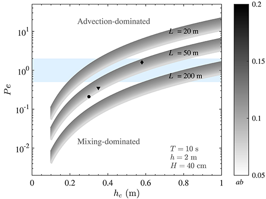
Figure 3. Variation of the Péclet number with canopy height (h_c) and dimensionless frontal area (ab). Variables held constant are indicated in the figure. The blue band represents Pe ~ O(1). The Péclet number of real canopies span a wide range and a small variation in the canopy height can lead to significant changes in Pe. The black diamond, triangle, and circle markers represent estimated values of Pe of canopies shown in Figures 2A–C, respectively, highlighting that real canopies can fall within the Pe < 1, Pe > 1, or Pe ~ O(1) regimes.

A summary of the framework developed here is presented as a flowchart in Figure 4. The key input values include canopy (i.e., L_D) and wave (h, H, and T) properties, with which ΔU (from Lowe et al., 2005) and ξ_T (using Equation 5) can be calculated. We can then estimate T_mix and T_adv and ultimately Pe through Equations (1) to (8). When Pe ≫ 1, T_res ≈ T_adv and Equation (7) can be used for calculating residence time. When Pe ≪ 1, T_res ≈ T_mix and Equation (6) can be used for calculating residence time. When Pe ~ O(1), T_mix is the same order of magnitude of T_adv, and either diffusion or advection time scale can be used as an approximation of the residence time of the system (within one order of magnitude estimate). This is examined in the following section, where variations of T_res with ranges of wave (H and h) and canopy (ab and h_c) parameters are depicted.

FIGURE 4

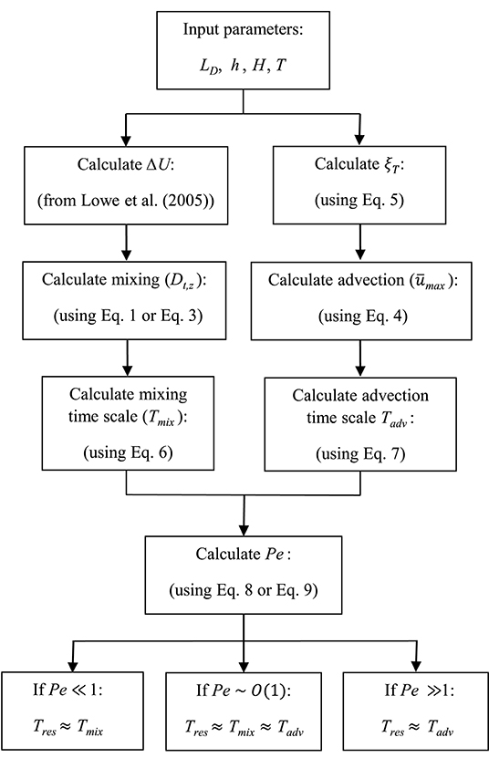
Figure 4. Flowchart representing the framework developed here for estimating residence time in coastal canopies. The input values include wave (h, H, and T) and canopy (L_D) properties. Using the model developed in Lowe et al. (2005) (to calculate ΔU) and Equations (1) to (8), this framework represents predictive estimation of residence time in submerged canopies under wave-dominated flows.

3. Results

For all calculations here, typical ranges of wave and canopy properties were selected. For a given canopy height and for conditions examined in each particular analysis in Figures 5A–C, a short canopy with L < 20 m always falls within the advection-dominated regime, a long canopy with L > 200 m falls within the mixing-dominated regime, and a medium-sized canopy with 20 < L < 200 falls in between the two (results not shown). Thus, L = 20 m and L = 200 m were chosen as representatives of advection- and mixing-dominated regimes, respectively. A medium canopy with L = 50 m was chosen in Figure 5D as the representative of conditions where a canopy experiences the transitional regime. The selection of these canopy lengths would also avoid overlapping of residence time values for mixing- and advection-dominated environments in each plot, providing more clarity and a better visual judgement of the results for each particular case. Constant values employed for calculations in each panel are indicated in the legends.

FIGURE 5

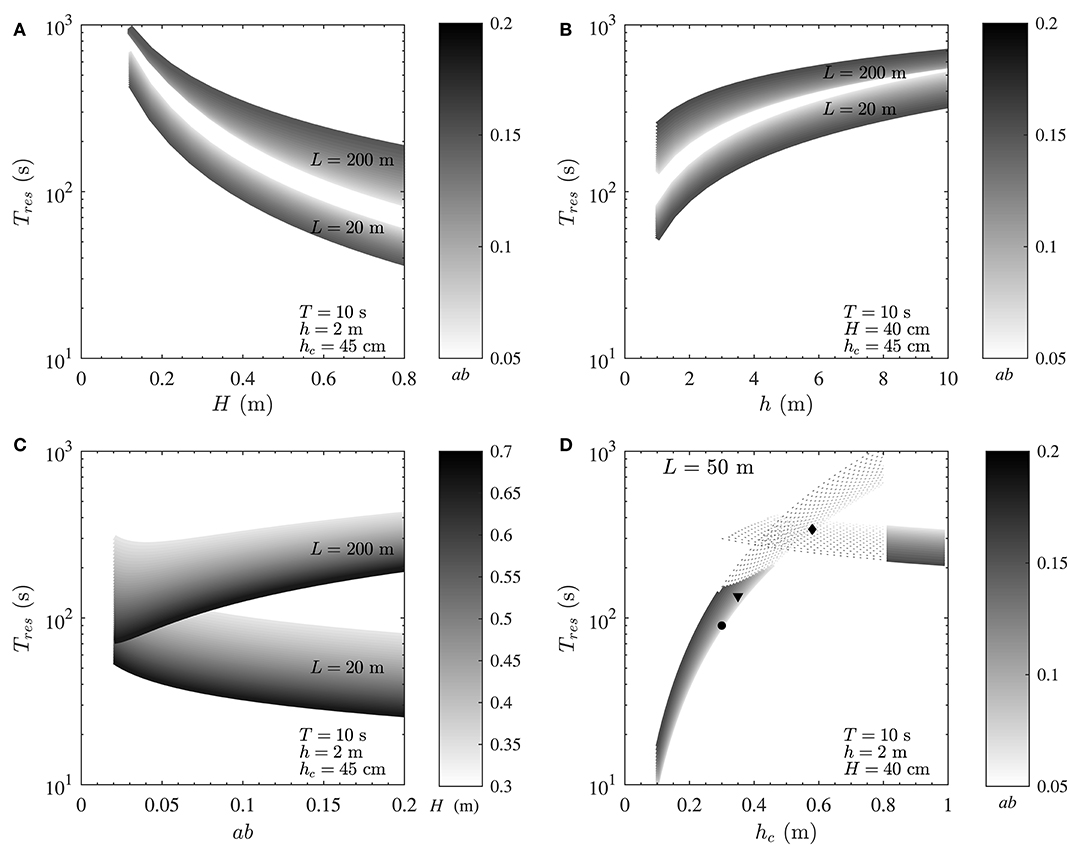
Figure 5. Variation of residence time with wave and canopy properties for a typical seagrass meadow. (A) Residence time decreases with increasing wave height (H), and (B) increases with water depth (h) (in both mixing- and advection-dominated canopies). (C) While residence time decreases with canopy density (ab) in short, mixing-dominated canopies, it increases in long, advection-dominated canopies. (D) Increasing canopy height enhances residence time until reaching a threshold value after which T_res decreases with increasing canopy height (h_c). The black diamond, triangle, and circle represent values of T_res in the canopies shown in Figures 2A–C, respectively. Constant variables for calculations of each plot are indicated in the figure.

3.1. Variation of Residence Time With Wave Height

First, consider the variation of residence time with wave height (Figure 5A); residence time decreases simply with increasing wave height, in both mixing- and advection-dominated canopies. This reduction, which can be as high as an order of magnitude, is due to the enhancement of both mixing and advection with wave height and ultimately wave orbital velocity as can be inferred from Equations (3) and (4). The significant impact of the canopy length is also noteworthy; a shorter canopy will invariably have a lower residence time compared to a longer canopy, irrespective of the wave height and canopy density.

3.2. Variation of Residence Time With Water Depth

Now consider situations where the wave height is constant (Figure 5B); based on linear wave theory, the magnitude of wave velocity decreases with increasing water depth ($U_{\infty }\approx 0.5\text{H}\sqrt{(g/h)}$), with g being gravitational acceleration), resulting in diminished vertical mixing (Equations 1, 3) and horizontal flushing (Equation 4). This ultimately impacts positively on the magnitude of T_res such that residence time increases with water depth in both mixing- and advection-dominated environments. Consistent with Figure 5A, increasing canopy density (ab) decreases residence time in short, advection-dominated canopies and increases residence time in long, mixing-dominated canopies. This is further investigated in the following section.

3.3. Variation of Residence Time With Canopy Density

In contrast to wave height and water depth, residence time does not vary simply with changes in canopy density (represented here by ab) in mixing- and advection-dominated environments (Figure 5C). In particular, in mixing-dominated canopies (L ≥ 200 m), residence time increases monotonically with ab for constant water depth and wave period. This is due to the reduction of both wake- and shear-driven mixing in dense canopies (due to the diminished in-canopy velocity, see Abdolahpour et al., 2017a). In small patches, where advection is dominant (≤ 20 m), T_res decreases with increasing canopy density, due to the enhancement of canopy drag and ultimately ${\overline{u}}_{max}$ (Equation 4).

3.4. Variation of Residence Time With Canopy Height

As shown in Figure 3, a small variation in canopy height can have a significant impact on the transport regime. To demonstrate how changes in canopy height would impact residence time, a medium size canopy with L = 50 m (with Pe ~ O(1), which would also experience the transitional regime) was chosen (Figure 5D). In this example, for shorter canopy heights (h_c ≲ 40 cm), the flow is mixing-dominated (Pe ≪ 1, Figure 3) and for taller canopies (h_c≳80 cm), the flow is advection-dominated (Pe≫1, Figure 3). For canopies with 40 cm ≲ h_c ≲ 80 cm, Pe ~ O(1) and both mixing and advection can be equally important. The dashed lines in Figure 5D show the magnitude of T_mix and T_adv within the transitional regime. As seen, advective and diffusive timescales are of the same order in this regime, and either T_adv or T_mix can be used for a first order estimate of residence time, depending on the availability of key canopy and wave parameters. Moreover, predicted values of residence time for canopies shown in Figure 2 are also shown in Figure 5D (black diamond, triangle and circle, respectively). It is noteworthy that canopy residence time is so strongly governed by canopy properties that slight morphological changes in these canopies lead to a significant variation (by a factor of 3) of the residence time.

While the results presented here nicely demonstrate how residence time varies in a typical coastal canopy, the method described in section 2 (also, summarized in Figure 4) must be followed for residence time estimation for specific wave and canopy conditions.

Here, we present an analytic framework to estimate the dominant residence timescale in coastal canopies across a wide range of wave and canopy properties. The sensitivity of the health and function of a given system to the residence time within the canopy depends entirely on the ecological and biogeochemical processes of interest. For applications requiring an accuracy of seconds or smaller, a highly sophisticated numerical model will be needed to predict a precise residence time.

4. Discussion

The framework developed here allows predictive estimation of the canopy residence time, relevant to many significant ecological processes, under a wide range of wave and canopy conditions. Table 2 presents values of residence time inside a canopy of Sargassum fusiforme (Harvey) Setchell exposed to high energy wave conditions (data from Nishihara et al., 2011) along with predicted values of residence time in the same canopy, using the model developed here. As seen, the predicted values are in excellent agreement (in order of magnitude terms) with those observed in the real coastal canopies. To the best of our knowledge, this is the only available field measurement of residence time in coastal, and thus, wave-dominated canopies. There have been a limited number of previous studies where material residence time has been measured directly within submerged and emergent macrophyte canopies under current-dominated environments. Table 2 summarizes key system characteristics and residence times observed in these studies. Although a direct comparison between our model predictions (developed for wave-dominated environments) and residence times measured in current-dominated canopies is not straightforward, canopy residence timescales predicted here are quite comparable [i.e., O(100 s)] to available field estimates in such systems. An essentially-important next step is to assess model predictions in real systems, where a wider range of canopy and hydrodynamic complexities are present.

TABLE 2

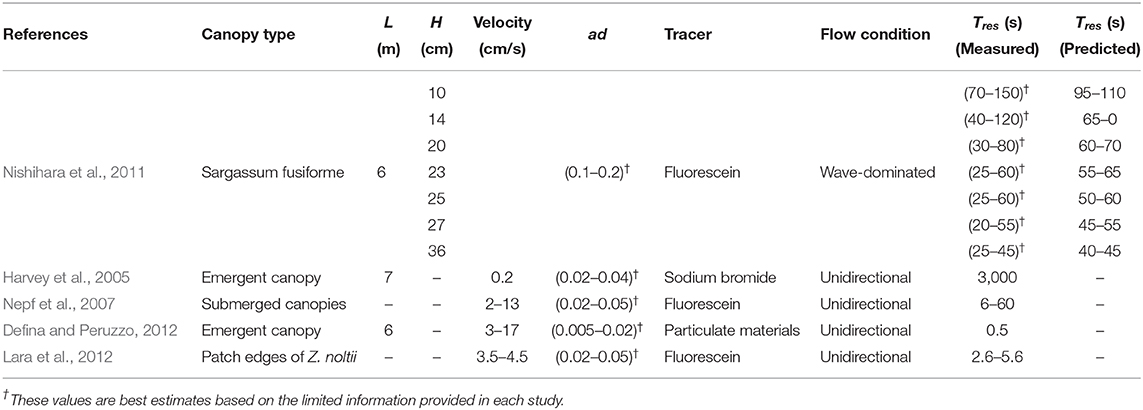
Table 2. Available field measurements of canopy residence time.

While direct field measurements of canopy residence time and its impact on biological and biogeochemical processes inside the canopy are extremely limited, there is a large number of studies from which an indirect impact of residence time on such processes can be inferred. For example, it has been shown that the morphological characteristics of the canopy (branch spacing, shapes, intra-canopy complexity, etc.) can have a profound impact on the rate of food intake in suspension-feeders (Riisgård et al., 2007; Brun et al., 2009), mass flux (Helmuth et al., 1997), and macroinvertebrate density inside the canopy (Gartner et al., 2013). This can plausibly be explained by the indirect effects of the variation of the canopy residence time (due to the presence of canopies or changes in their structural properties) on such biological and ecological processes. Moreover, there are a number of studies that have investigated the relative importance of turbulent mixing and advection on important ecological processes and their indirect impact on canopy morphology. These studies suggest that the dominant transport mechanism (whether it is mixing or advection), can also have a non-negligible impact on structural adaptations of the canopy. For example, the morphological characteristics of aggregates in stony corals drastically change with the Péclet number (Kaandorp et al., 1996). In particular, stony corals have more compact cluster shapes when Pe ≫ 1 (or advection-dominated environments) and more branching shapes when Pe ≪ 1 (or diffusion-dominated environments). This morphological adaptation was related to the variation of residence time and thus nutrient availability in each transport regime, further highlighting the importance of being able to predict canopy residence times for understanding biogeochemical cycling within the canopy.

Results obtained here also revealed that residence time in real coastal canopies may vary significantly, from orders of seconds to hours. This variation is strongly related to wave and canopy properties such that a slight change in the canopy morphology may result in a significant alteration in the residence time (see e.g., Figure 5C). This has considerable ecological implications for marine habitats through the direct impact on a range of ecological and environmental processes within the canopy. In particular, a longer residence time provides a longer exposure time and therefore greater material availability for active surfaces. Previous studies have employed the Damköhler number (Da), a dimensionless parameter that represents the ratio of exposure and processing timescales to characterize the dynamics of the system. When Da ≪ 1, the exposure timescale (which is equivalent to T_res) is much less than the processing timescale and the material does not have sufficient time to react during the transport (i.e., a conservative system). For filter feeding organisms living in a canopy this would mean that there is not sufficient time for the organism to filter the particles out of the water before they are advected (or diffused) out of the system. Similarly, for seagrasses, there is insufficient time to take up dissolved nutrients through the leaf surface. In contrast, values of Da ≫ 1 indicate that the exposure timescale is longer than the processing timescale, and filter feeders and seagrasses would have adequate time to remove particles or nutrients from the water column (i.e., a reactive system). When Da ~ O(1), the system is considered highly dynamic and the balance between being conservative or reactive, is greatly sensitive to changes in wave and canopy conditions (Oldham et al., 2013).

To demonstrate how changes in residence time may impact ecological and biogeological processes inside the canopy, values of Da from a range of studies are presented as a function of the Keulegan-Carpenter number (KC) in Figure 6. The Keulegan-Carpenter number is a dimensionless parameter that represents the relative magnitude of wave horizontal excursion (A_∞) to drag length scale (L_D) and can be calculated as:

$\begin{array}{ll}KC=\frac{U_{\infty }^{rms}T}{L_D}& (10)\end{array}$

Since this parameter encompasses both wave and canopy properties, it can conveniently be used as a generalized parameter to represent canopy-wave interactions of each system. In particular, KC controls the in-canopy oscillatory flow and, when small, is indicative of rapidly reversing flow and, when very large, is more dynamically similar to unidirectional flow. Thus, it is an ideal (and relevant) parameter to investigate the variation of Da with wave and canopy properties. Here, we present Da for the process of nutrient uptake in a wide range of canopies, including corals (Atkinson et al., 2001), seagrass meadows (Thomas and Cornelisen, 2003), and macroalgae (Weitzman et al., 2013). The processing time scales for nutrient uptake in each canopy have been calculated using the uptake rate constant and the method developed by Pujol et al. (2019). Values of residence time for each canopy and wave condition have also been predicted using the model developed here.

FIGURE 6

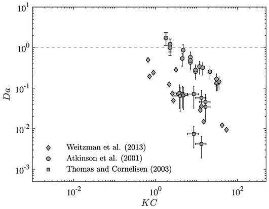
Figure 6. Variation of Damköhler number (Da) with Keulegan-Carpenter number (KC). Values of Da calculated for nutrient uptake in canopies of corals (Atkinson et al., 2001), seagrasses (Weitzman et al., 2013), and macroalgae (Thomas and Cornelisen, 2003). Changes in wave and canopy properties (represented here by KC) lead to variation of nutrient uptake from dynamic to conservative environment. Vertical bars represent the standard deviation of Da estimates.

As seen in Figure 6, Da in the canopies examined here can span a wide range [Da ~ O(0.01−1)]. Moreover, any variation in wave and canopy conditions (represented here by KC) may have a significant impact on the canopy uptake rate such that changes in KC can lead a canopy to transition between conservative and reactive states. Note, these results only represent the range of uptake rate for the canopies examined here. Real coastal canopies may experience a wider range of uptake rate (or Da) when wave and canopy properties vary from season to season or location to location.

Finally, it is important to note that the efficiency of mixing processes and, therefore, the overall residence time is tightly controlled by numerous factors and complexities present in natural systems such as particle characteristics (e.g., seeds, pollen, larvae, and sediment) and canopy intra-diversities. Further, this study examines flow and mixing in canopies exposed to (idealized) monochromatic sinusoidal waves. Thus, although the framework developed here allows predictive estimation of the canopy residence timescales for a wide and realistic range of wave and canopy properties, a fundamentally-important next step is testing the framework developed here in the complexity of a real multi-specific coastal canopy across a wider range of wave conditions.

5. Conclusion

Quantification of the Péclet number (Pe), the ratio of diffusive to advective time scales, simplifies the prediction of residence time in typical coastal canopies. This can be done through classification of coastal canopies into three distinct environments; i.e., (a) mixing-dominated exchange (Pe ≪ 1), (b) advection-dominated exchange (Pe ≫ 1), and (c) a transitional regime [Pe ~ O(1)]. The framework developed here has enabled predictions of dominant residence timescales in all three regimes. Further, the results obtained here revealed that canopy residence time depends heavily on wave and canopy properties and may vary significantly (from orders of seconds to hours) from season to season or location to location. Finally, while there is reasonably good agreement between model predictions and available field measurements, testing of the model presented here for a wide range of field conditions is a critically important next step.

Data Availability Statement

The datasets analyzed for this study can be obtained by sending a written request to the corresponding author at maryam.abdolahpour@uwa.edu.au.

Author Contributions

MA undertook the literature review, model development, data analysis, and manuscript writing. MG provided advice on model development, data analysis, and interpretation as well as manuscript writing. PL and KM provided input into research design and assisted with interpretation of results for ecological and biological implications. All authors contributed to the article and approved the submitted version.

Funding

This research was supported by the Australian Government through the Australian Research Council's Discovery Projects funding scheme (project DP170100802) and a grant from the Australian Department of Innovation, Industry, Science, and Research's Collaborative Research Network Scheme (Grant CRN2011:05).

Conflict of Interest

The authors declare that the research was conducted in the absence of any commercial or financial relationships that could be construed as a potential conflict of interest.

References

Abdolahpour, M. (2017). Residence time in coastal canopies (Ph.D. thesis). Perth: The University of Western Australia; Edith Cowan University.

Google Scholar

Abdolahpour, M., Ghisalberti, M., Lavery, P., and McMahon, K. (2017a). Vertical mixing in coastal canopies. Limnol. Oceanogr. 62, 26–42. doi: 10.1002/lno.10368

CrossRef Full Text | Google Scholar

Abdolahpour, M., Ghisalberti, M., McMahon, K., and Lavery, P. (2018). The impact of flexibility on flow, turbulence and vertical mixing in coastal canopies. Limnol. Oceanogr. 63, 2777–2792. doi: 10.1002/lno.11008

CrossRef Full Text | Google Scholar

Abdolahpour, M., Hambleton, M., and Ghisalberti, M. (2017b). The wave-driven current in coastal canopies. J. Geophys. Res. Ocean 122, 3660–3674. doi: 10.1002/2016JC012446

CrossRef Full Text | Google Scholar

Ackerman, J. D. (2002). Diffusivity in a marine macrophyte canopy: implications for submarine pollination and dispersal. Am. J. Bot. 89, 1119–1127. doi: 10.3732/ajb.89.7.1119

PubMed Abstract | CrossRef Full Text | Google Scholar

Atkinson, M., Falter, J., and Hearn, C. (2001). Nutrient dynamics in the biosphere 2 coral reef mesocosm: water velocity controls NH 4 and PO 4 uptake. Coral Reefs 20, 341–346. doi: 10.1007/s00338-001-0184-7

CrossRef Full Text | Google Scholar

Brun, F. G., Zetten, E., Cacabelos, E., and Bouma, T. J. (2009). Role of two contrasting ecosystem engineers (Zostera noltii and Cymodocea nodosa) on the food intake rate of Cerastoderma edule. Helgoland. Mar. Res. 63:19. doi: 10.1007/s10152-008-0134-7

CrossRef Full Text | Google Scholar

Bulthuis, D. A., and Woelkerling, W. M. (1983). Seasonal variation in standing crop, density and leaf growth rate of the Seagrass, heterozostera tasmanica, in western port and port Phillip Bay, Victoria, Australia. Aquat. Bot. 16, 111–136. doi: 10.1016/0304-3770(83)90088-8

CrossRef Full Text | Google Scholar

Cambridge, M. L., and Kuo, J. (1979). Two new species of Seagrasses from Australia, Posidonia sinuosa and P. angustifolia (posidoniaceae). Aquat. Bot. 6, 307–328. doi: 10.1016/0304-3770(79)90071-8

CrossRef Full Text | Google Scholar

Collier, C. J., Lavery, P. S., Masini, R. J., and Ralph, P. J. (2007). Morphological, growth and meadow characteristics of the seagrass Posidonia sinuosa along a depth-related gradient of light availability. Mar. Ecol. Prog. Ser. 337, 103–115. doi: 10.3354/meps337103

CrossRef Full Text | Google Scholar

Collier, C. J., Lavery, P. S., Ralph, P. J., and Masini, R. J. (2009). Shade-induced response and recovery of the seagrass Posidonia sinuosa. J. Exp. Mar. Biol. Ecol. 370, 89–103. doi: 10.1016/j.jembe.2008.12.003

CrossRef Full Text | Google Scholar

Connolly, R. M., Hindell, J. S., and Gorman, D. (2005). Seagrass and epiphytic algae support nutrition of a fisheries species, Sillago schomburgkii, in adjacent intertidal habitats. Mar. Ecol. Prog. Ser. 286, 69–79. doi: 10.3354/meps286069

CrossRef Full Text | Google Scholar

Dean, R., and Dalrymple, R. (1991). Water Wave Mechanics for Scientists and Engineers. Advanced Series in Ocean Engineering. Hackensack, NJ: World Sci. Publ.

Google Scholar

Defina, A., and Peruzzo, P. (2012). Diffusion of floating particles in flow through emergent vegetation: further experimental investigation. Water. Resour. Res. 48, 1–11. doi: 10.1029/2011WR011147

CrossRef Full Text | Google Scholar

Duarte, C. M. (2002). The future of seagrass meadows. Environ. Conserv. 29, 192–206. doi: 10.1017/S0376892902000127

CrossRef Full Text | Google Scholar

Falter, J. L., Atkinson, M. J., and Merrifield, M. A. (2004). Mass-transfer limitation of nutrient uptake by a wave-dominated reef flat community. Limnol. Oceanogr. 49, 1820–1831. doi: 10.4319/lo.2004.49.5.1820

CrossRef Full Text | Google Scholar

Fonseca, M. S., and Cahalan, J. A. (1992). A preliminary evaluation of wave attenuation by four species of seagrass. Estuar. Coast. Shelf. Sci. 35, 565–576. doi: 10.1016/S0272-7714(05)80039-3

CrossRef Full Text | Google Scholar

Fonseca, M. S., Kenworthy, W. J., and Thayer, G. W. (1992). “Seagrass beds: nursery for coastal species,” in Stemming the Tide of Coastal Fish Habitat Loss. Marine Recreational Fisheries Symposium (Baltimore, MD), 141–147.

Google Scholar

Gacia, E., Duarte, C. M., and Middelburg, J. J. (2002). Carbon and nutrient deposition in a Mediterranean Seagrass (Posidonia oceanica) meadow. Limnol. Oceanogr. 47, 23–32. doi: 10.4319/lo.2002.47.1.0023

CrossRef Full Text | Google Scholar

Gacia, E., Granata, T., and Duarte, C. (1999). An approach to measurement of particle flux and sediment retention within Seagrass (Posidonia oceanica) meadows. Aquat. Bot. 65, 255–268. doi: 10.1016/S0304-3770(99)00044-3

CrossRef Full Text | Google Scholar

Gambi, M. C., Nowell, A. R., and Jumars, P. (1990). Flume observations on flow dynamics in Zostera marina (eelgrass) beds. Mar. Ecol. Prog. Ser. Oldendorf 61, 159–169. doi: 10.3354/meps061159

CrossRef Full Text | Google Scholar

Gartner, A., Tuya, F., Lavery, P. S., and McMahon, K. (2013). Habitat preferences of macroinvertebrate fauna among seagrasses with varying structural forms. J. Exp. Mar. Biol. Ecol. 439, 143–151. doi: 10.1016/j.jembe.2012.11.009

CrossRef Full Text | Google Scholar

Ghisalberti, M., and Nepf, H. (2005). Mass transport in vegetated shear flows. Environ. Fluid Mech. 5, 527–551. doi: 10.1007/s10652-005-0419-1

CrossRef Full Text | Google Scholar

Ghisalberti, M., and Schlosser, T. (2013). Vortex generation in oscillatory canopy flow. J. Geophys. Res. Ocean 118, 1534–1542. doi: 10.1002/jgrc.20073

CrossRef Full Text | Google Scholar

Granata, T., Serra, T., Colomer, J., Casamitjana, X., Duarte, C., Gacia, E., et al. (2001). Flow and particle distributions in a nearshore seagrass meadow before and after a storm. Mar. Ecol. Prog. Ser. 218, 95–106. doi: 10.3354/meps218095

CrossRef Full Text | Google Scholar

Harvey, J. W., Conklin, M. H., and Koelsch, R. S. (2003). Predicting changes in hydrologic retention in an evolving semi-arid alluvial stream. Adv. Water. Resour. 26, 939–950. doi: 10.1016/S0309-1708(03)00085-X

CrossRef Full Text | Google Scholar

Harvey, J. W., Saiers, J. E., and Newlin, J. T. (2005). Solute transport and storage mechanisms in wetlands of the everglades, South Florida. Water. Resour. Res. 41, 1–14. doi: 10.1029/2004WR003507

CrossRef Full Text | Google Scholar

Helmuth, B., and Sebens, K. (1993). The influence of colony morphology and orientation to flow on particle capture by the scleractinian coral agaricia agaricites (linnaeus). J. Exp. Mar. Biol. Ecol. 165, 251–278. doi: 10.1016/0022-0981(93)90109-2

CrossRef Full Text | Google Scholar

Helmuth, B. S., Sebens, K. P., and Daniel, T. L. (1997). Morphological variation in coral aggregations: branch spacing and mass flux to coral tissues. J. Exp. Mar. Biol. Ecol. 209, 233–259. doi: 10.1016/S0022-0981(96)02687-1

CrossRef Full Text | Google Scholar

Infantes, E., Terrados, J., Orfila, A., Ca nellas, B., and Álvarez-Ellacuria, A. (2009). Wave energy and the upper depth limit distribution of posidonia oceanica. Bot. Mar. 52, 419–427. doi: 10.1515/BOT.2009.050

CrossRef Full Text | Google Scholar

Kaandorp, J. A., Lowe, C. P., Frenkel, D., and Sloot, P. M. (1996). Effect of nutrient diffusion and flow on coral morphology. Phys. Rev. Lett. 77:2328. doi: 10.1103/PhysRevLett.77.2328

PubMed Abstract | CrossRef Full Text | Google Scholar

Kendrick, G. A., Duarte, C. M., and Marbà, N. (2005). Clonality in seagrasses, emergent properties and seagrass landscapes. Mar. Ecol. Prog. Ser. 290, 291–296. doi: 10.3354/meps290291

CrossRef Full Text | Google Scholar

Kobayashi, N., Raichle, A. W., and Asano, T. (1993). Wave attenuation by vegetation. J. Waterw. Port Coast. Ocean Eng. 119, 30–48. doi: 10.1061/(ASCE)0733-950X(1993)119:1(30)

CrossRef Full Text | Google Scholar

Koch, E. W., Sanford, L. P., Chen, S.-N., Shafer, D. J., and Smith, J. M. (2006). Waves in Seagrass Systems: Review and Technical Recommendations. Technical report, DTIC Document.

Google Scholar

Lara, M., Peralta, G., Alonso, J., Morris, E. P., González-Ortiz, V., Rueda-Márquez, J., et al. (2012). Effects of intertidal seagrass habitat fragmentation on turbulent diffusion and retention time of solutes. Mar. Pollut. Bull. 64, 2471–2479. doi: 10.1016/j.marpolbul.2012.07.044

PubMed Abstract | CrossRef Full Text | Google Scholar

Larkum, A., Orth, R. J., and Duarte, C. M. (2006). Seagrasses: Biology, Ecology and Conservation. Springers; Dordrecht.

Google Scholar

Lowe, R. J., Koseff, J. R., and Monismith, S. G. (2005). Oscillatory flow through submerged canopies: 1. velocity structure. J. Geophys. Res. Ocean 110, 1–17. doi: 10.1029/2004JC002788

CrossRef Full Text | Google Scholar

Luhar, M., Coutu, S., Infantes, E., Fox, S., and Nepf, H. (2010). Wave-induced velocities inside a model seagrass bed. J. Geophys. Res. Ocean. 115, 1–15. doi: 10.1029/2010JC006345

CrossRef Full Text | Google Scholar

Luhar, M., Infantes, E., Orfila, A., Terrados, J., and Nepf, H. M. (2013). Field observations of wave-induced streaming through a submerged seagrass (Posidonia oceanica) meadow. J. Geophys. Res. Ocean 118, 1955–1968. doi: 10.1002/jgrc.20162

CrossRef Full Text | Google Scholar

Mohring, M., and Rule, M. (2014). A Survey of Selected Seagrass Meadows in Cockburn Sound, Owen Anchorage and Warnbro Sound. Data Report prepared for Cockburn Sound Management Council, 1–49.

Google Scholar

Moore, K. A. (2004). Influence of seagrasses on water quality in shallow regions of the lower Chesapeake Bay. J. Coast. Res. 10045, 162–178. doi: 10.2112/SI45-162.1

CrossRef Full Text | Google Scholar

Morris, E. P., Peralta, G., Brun, F. G., Van Duren, L., Bouma, T. J., and Perez-Llorens, J. L. (2008). Interaction between hydrodynamics and seagrass canopy structure: spatially explicit effects on ammonium uptake rates. Limnol. Oceanogr. 53, 1531–1539. doi: 10.4319/lo.2008.53.4.1531

CrossRef Full Text | Google Scholar

Nepf, H., Ghisalberti, M., White, B., and Murphy, E. (2007). Retention time and dispersion associated with submerged aquatic canopies. Water Resour. Res. 43, 1–10. doi: 10.1029/2006WR005362

CrossRef Full Text | Google Scholar

Nishihara, G. N., Terada, R., and Shimabukuro, H. (2011). Effects of wave energy on the residence times of a fluorescent tracer in the canopy of the intertidal marine macroalgae, Sargassum fusiforme (Phaeophyceae). Phycol. Res. 59, 24–33. doi: 10.1111/j.1440-1835.2010.00595.x

CrossRef Full Text | Google Scholar

Oldham, C., Farrow, D., and Peiffer, S. (2013). A generalized damköhler number for classifying material processing in hydrological systems. Hydrol. Earth Syst. Sci. 17, 1133–1148. doi: 10.5194/hess-17-1133-2013

CrossRef Full Text | Google Scholar

Oreska, M. P., McGlathery, K. J., and Porter, J. H. (2017). Seagrass blue carbon spatial patterns at the meadow-scale. PLoS ONE 12:e0176630. doi: 10.1371/journal.pone.0176630

PubMed Abstract | CrossRef Full Text | Google Scholar

Orth, R. J., Luckenbach, M., and Moore, K. A. (1994). Seed dispersal in a marine macrophyte: implications for colonization and restoration. Ecology 75, 1927–1939. doi: 10.2307/1941597

CrossRef Full Text | Google Scholar

Pujol, D., Abdolahpour, M., Lavery, P. S., McMahon, K., and Oldham, C. (2019). Flow velocity and nutrient uptake in marine canopies. Mar. Ecol. Prog. Ser. 622, 17–30. doi: 10.3354/meps12987

CrossRef Full Text | Google Scholar

Pujol, D., Serra, T., Colomer, J., and Casamitjana, X. (2013). Flow structure in canopy models dominated by progressive waves. J. Hydrol. 486, 281–292. doi: 10.1016/j.jhydrol.2013.01.024

CrossRef Full Text | Google Scholar

Reidenbach, M. A., Koseff, J. R., and Monismith, S. G. (2007). Laboratory experiments of fine-scale mixing and mass transport within a coral canopy. Phys. Fluids 19:075107. doi: 10.1063/1.2752189

CrossRef Full Text | Google Scholar

Riisgård, H. U., Lassen, J., Kortegaard, M., Møller, L. F., Friedrichs, M., Jensen, M. H., and Larsen, P. S. (2007). Interplay between filter-feeding zoobenthos and hydrodynamics in the shallow Odense fjord (Denmark)-earlier and recent studies, perspectives and modelling. Estuar. Coast. Shelf. Sci. 75, 281–295. doi: 10.1016/j.ecss.2007.04.032

CrossRef Full Text | Google Scholar

Rosman, J. H., Koseff, J. R., Monismith, S. G., and Grover, J. (2007). A field investigation into the effects of a kelp forest (Macrocystis pyrifera) on coastal hydrodynamics and transport. J. Geophys. Res. Ocean 112, 1–16. doi: 10.1029/2005JC003430

CrossRef Full Text | Google Scholar

Scott, L. C., Boland, J. W., Edyvane, K. S., and Jones, G. (2000). Development of a seagrass-fish habitat model-I: a seagrass residency index for economically important species. Environmetrics 11, 541–552. doi: 10.1002/1099-095X(200009/10)11:5<541::AID-ENV416>3.0.CO;2-A

CrossRef Full Text | Google Scholar

Sebens, K. P., Witting, J., and Helmuth, B. (1997). Effects of water flow and branch spacing on particle capture by the reef coral madracis mirabilis (duchassaing and michelotti). J. Exp. Mar. Biol. Ecol. 211, 1–28. doi: 10.1016/S0022-0981(96)02636-6

CrossRef Full Text | Google Scholar

Thomas, F. I., and Cornelisen, C. D. (2003). Ammonium uptake by seagrass communities: effects of oscillatory versus unidirectional flow. Mar. Ecol. Prog. Ser. 247, 51–57. doi: 10.3354/meps247051

CrossRef Full Text | Google Scholar

van Rooijen, A., Lowe, R., Rijnsdorp, D., Ghisalberti, M., Jacobsen, N. G., and McCall, R. (2020). Wave-driven mean flow dynamics in submerged canopies. J. Geophys. Res. 125, 1–21. doi: 10.1029/2019JC015935

CrossRef Full Text | Google Scholar

Weitzman, J., Aveni-Deforge, K., Koseff, J., and Thomas, F. (2013). Uptake of dissolved inorganic nitrogen by shallow seagrass communities exposed to wave-driven unsteady flow. Mar. Ecol. Prog. Ser. 475, 65–83. doi: 10.3354/meps09965

CrossRef Full Text | Google Scholar

Worcester, S. (1995). Effects of eelgrass beds on advection and turbulent mixing in low current and low shoot density environments. Mar. Ecol. Prog. Ser. 126, 223–232. doi: 10.3354/meps126223

CrossRef Full Text | Google Scholar

Zarnetske, J. P., Haggerty, R., Wondzell, S. M., and Baker, M. A. (2011). Dynamics of nitrate production and removal as a function of residence time in the hyporheic zone. J. Geophys. Res. Biogeosci. 116, 1–12. doi: 10.1029/2010JG001356

CrossRef Full Text | Google Scholar