Quantifying Marine Sedimentary Carbon: A New Spatial Analysis Approach Using Seafloor Acoustics, Imagery, and Ground-Truthing Data in Scotland

Hunt, Corallie; Demšar, Urška; Dove, Dayton; Smeaton, Craig; Cooper, Rhys; Austin, William E. N.

doi:10.3389/fmars.2020.00588

ORIGINAL RESEARCH article

Front. Mar. Sci., 28 July 2020

Sec. Coastal Ocean Processes

Volume 7 - 2020 | https://doi.org/10.3389/fmars.2020.00588

Quantifying Marine Sedimentary Carbon: A New Spatial Analysis Approach Using Seafloor Acoustics, Imagery, and Ground-Truthing Data in Scotland

$\r\nCorallie Hunt*$ Corallie Hunt^1*

Urška Demšar¹

Dayton Dove²

Craig Smeaton¹

Rhys Cooper²

William E. N. Austin^1,3

¹School of Geography and Sustainable Development, University of St Andrews, St Andrews, United Kingdom
²The Lyell Centre, British Geological Survey, Edinburgh, United Kingdom
³Scottish Association for Marine Science, Scottish Marine Institute, Oban, United Kingdom

Marine sediments are important repositories of organic matter, effectively burying organic carbon (OC) over geological timescales thus providing a climate regulation service. However, the spatial distribution of this marine sedimentary OC store is not well constrained. In this study we leverage a high resolution multibeam echosounder (MBES) survey taken at Loch Creran, a model fjordic site on the west coast of Scotland, to develop a new methodology for predicting the distribution of OC in surface sediments. Using an integrated approach, we use MBES survey, video imagery and ground-truthing data to produce a high-resolution (2 × 2 m) map of surficial carbon and calculate a 10 cm stock. We find that the backscatter survey reliably uncovers a heterogeneous seabed and that OC correlates strongly with the MBES backscatter signal as a function of sediment composition. We estimate that there are approximately 12,346 ± 2,677 t of OC held within the top 10 cm of mixed sediments across the MBES survey area (7.96 km²; 60% of the total area), upscaled to 20,577 ± 4,462 t of OC across Loch Creran (13.27 km²). Normalised by area, we find that fine sediments with small fractions of sand and gravel hold more OC than homogenous fine sediments. This initial work proposes a novel methodological approach to using high resolution MBES surveys to improve the spatial mapping of sedimentary carbon (C) and identification of C hotspots, enabling consideration of this resource in sedimentary carbon accounting, seabed management and climate mitigation strategies.

Introduction

The continental shelf is a net sink for carbon dioxide (CO₂) with substantial long-term stores of C found in seabed sediments (Bauer et al., 2013). The shelf C store is composed of carbonate material together with significant amounts of OC. For instance, the North-West European continental shelf is predicted to store 476 Mt of OC in surficial sediments, however, there are large uncertainties within this estimate (ranging between 230 and 882 Mt) (Diesing et al., 2017). Reducing uncertainties is necessary to improve assessments of the marine contribution to national C stock estimates (Avelar et al., 2017). Recent first-order marine C inventories for Scotland, United Kingdom, highlight that the inshore sediments of the Scottish continental shelf, contain much larger OC stocks than the biological components, such as intertidal macroalgae and saltmarshes (Burrows et al., 2014, 2017). Several key areas for further investigation were recommended, one of which advocated for the development of methods to understand the spatial distribution of the sedimentary C store. While terrestrial C stores, such as forests, have been well-mapped and also have robust protocols for C stock assessments and accounting (Gibbs et al., 2007), relatively little of the seabed has been adequately mapped (Diesing et al., 2016). Currently, within Europe, the production of seabed substrate and habitat maps is being driven by international and national directives such as the EU Marine Strategy Framework Directive (MSFD) (Council Directive 2008/56/EC, 2008) and the EU Habitats Directive (Council Directive 92/43/EEC, 1992), and coordinated initiatives such as the European Commissions’ European Marine Observation and Data network (EMODnet) Geology project. However, there is currently limited research dedicated to the accurate mapping of the sedimentary C store. With a growing understanding of the role of the shelf seas in carbon storage (Kröger et al., 2018), sediment maps detailing OC have the potential to inform marine management strategies for the preservation of sedimentary C, which is vulnerable to disturbance, natural or otherwise (Almroth-Rosell et al., 2012; Van De Velde et al., 2018). Recent large-scale sedimentary OC maps are modelled from physical sample data via interpolation or machine learning approaches and provide a generalised picture of OC based on the predominant sediment types (Wilson et al., 2018). Associated uncertainty estimates are thus high over such large scales due to the low-density ground-truth data, for instance within the northern North Sea (Diesing et al., 2017).

Modern-day seabed mapping as incorporated into marine ecosystem characterisation increasingly relies on acoustic data. Through providing a spatially continuous, high-resolution measure of bathymetry (i.e., water depth) over potentially large geographic areas, multibeam echosounder surveys (MBES) are effective tools for resolving significant seabed features (e.g., Dove et al., 2016; Micallef et al., 2018). Perhaps more important for characterising seabed substrate however, analysis of the concomitant MBES backscatter (intensity of acoustic return) allows for predictions of seabed sediment composition, relying on the relationship between acoustic backscatter properties and sediment particle size (Brown et al., 2011; Lurton and Lamarche, 2015). Nevertheless, ground-truthing via physical sampling (Collier and Brown, 2005; Brown et al., 2019) or towed video systems (Brown and Collier, 2008; Che Hasan et al., 2014; Calvert et al., 2015) is still a necessary component of the process to validate and calibrate the acoustic data. As yet, there is no standardised calibration of backscatter data directly to sediment type and it is still an evolving area of research (Lamarche and Lurton, 2018).

The aim of this study is to explore the application of multibeam backscatter data to map the OC distributed within surface seabed sediments. Organic matter (OM) has an affinity for muddy, fine-grained sediments (Keil et al., 1994). Our method is based on the principle that seabed substrates can be predicted from backscatter data based on acoustic return, therefore the same principle could be applied to predicting soft, carbon-rich sediments. We use a standard seabed mapping technique to produce an innovative and detailed picture of surface C stocks. Our study leverages data from a high resolution MBES survey conducted in a sea loch on the west coast of Scotland. These fjordic inshore environments are known to be global hotspots for the burial and storage of OC (Smith et al., 2015; Smeaton et al., 2016). The confined nature of fjords (Howe et al., 2010; Bianchi et al., 2020) provides a more controlled environment to allow the development and testing of this novel approach to mapping sedimentary OC that could be applied to the wider marine environment. We use the results from a sampling campaign to elucidate the relationships between sediment grain size, acoustic backscatter and OC. We have produced a high-resolution sedimentary C map from backscatter that could offer the basis for development of more robust stock calculations for sedimentary C and inform marine management strategies for the protection of this natural capital resource (Luisetti et al., 2013).

Regional Setting

Study Area

Our study site is Loch Creran, a fjordic inlet on the west coast of Scotland (Figure 1). Loch Creran is connected to the larger Loch Linnhe via a constricted entrance at the Lynn of Lorn. Loch Creran exhibits typical fjordic characteristics whereby its length of 12.8 km is more than double its width, it has a restricted geomorphology and past glacial erosion has created over-deepened conditions (Smeaton et al., 2017). The average depth is 13.4 m reaching a maximum depth of 49 m in the lower basin. Although presently ice-free, Loch Creran is characterised by four basins which are separated by shallow underwater sills (between 3 and 15 m deep at low water) (Black et al., 2000), remnants of past glacial retreat and associated depositional processes (Howe et al., 2010; Bianchi et al., 2020). Sills are important topographic constraints influencing circulation within fjords and therefore the volume and speed of flow (Inall and Gillibrand, 2010). The river Creran flows into the head of the loch at the north-east corner providing an average freshwater supply of 286.3 × 10⁶ m³ yr^–1 and associated sediment loads from the catchment (Almroth-Rosell et al., 2012). Deposition of fluvial sediments is influenced by the bathymetric and hydrographic regimes operating within the loch and due to its relatively sheltered exposure to wave action, Loch Creran experiences high sedimentation rates and is a net sink for OM (Loh et al., 2010). Loch Creran is typically well-mixed (Black et al., 2000). Exchange with the coastal waters of Loch Linnhe occurs at the mouth of Loch Creran to the west with a flushing time of approximately 3 days (Almroth-Rosell et al., 2012), which prevents hypoxic conditions from developing within the loch (Gillibrand et al., 2006). Loch Creran has several marine features protected under European and national marine conservation designations, namely for biogenic and bedrock reef and flame shell beds. These features are highlighted to show restricted sampling locations within our site; see Figure 1 for further details.

FIGURE 1

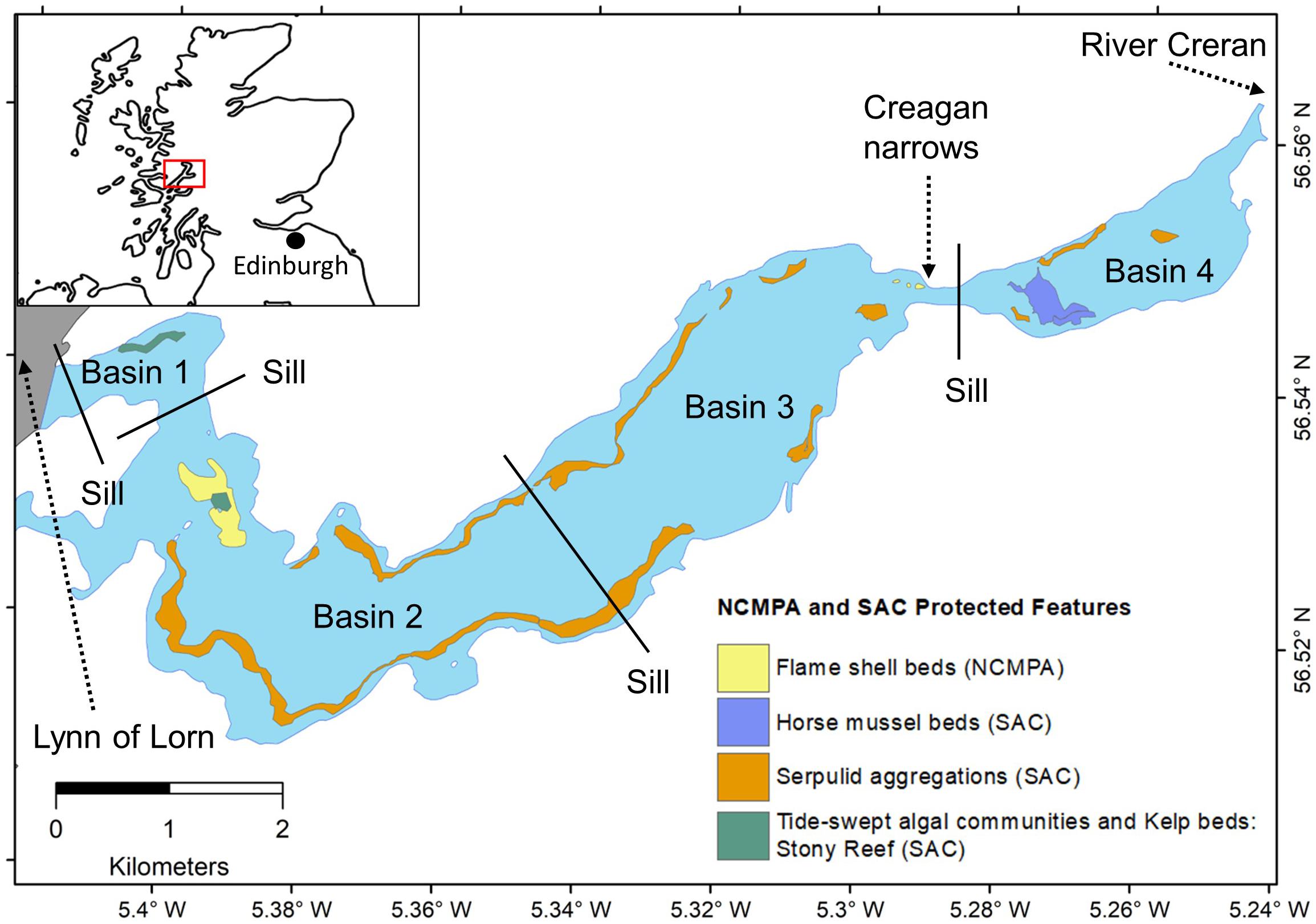
Figure 1. Location map for the study area. Loch Creran, on the west coast of Scotland, is highlighted in the red box (inset); The four basins and sill locations are indicated. Priority marine features protected under the EC Habitats Directive Special Area of Conservation (SAC EU Code: UK0030190) and Scottish Waters Nature Conservation Marine Protected Area (Loch Creran NCMPA) are highlighted to show the areas that were avoided during grab sampling. Map adapted from Black et al. (2000).

Materials and Methods

The following sections describe the suite of data that were used to develop a methodology that allows the spatial mapping of sedimentary OC within Loch Creran. Both qualitative and quantitative methods were used in this exploratory investigation.

Multi-Beam Echosounder Survey (MBES)

Acoustic data were collected by the British Geological Survey (BGS) in July 2017 in Loch Creran from the Research Vessel ‘White Ribbon’ using a vessel-mounted Kongsberg EM3002D dual-headed multibeam system logging 508 beams in the 300 kHz frequency range. The survey was undertaken at an average speed of 4–5 knots. Vessel positioning was achieved using a Trimble SPS461 with precise DGPS corrections provided via a Fugro MarineStar licence giving approximately 0.1 m navigational accuracy in the horizontal and 0.15 cm in the vertical planes. A Kongsberg Seatex Seapath 33 provided motion data. Sound velocity observations were recorded using a Valeport miniSVP probe and ranged between 1497 and 1501 m/s during the survey. Tidal data were corrected to the Vertical Offshore Reference Frame (VORF). The data were processed at the BGS in accordance with the standard UK Hydrographic Office (UKHO) Standard Operating Procedure (SOP) for Kongsberg Maritime multibeam data using CARIS HIPS v9.1 software. Data were automatically processed using the Combined Uncertainty and Bathymetry Estimator (CUBE) algorithm, with a cube surface at 1 m resolution produced for the entire survey area. Final bathymetric products were output using Fledermaus and ArcGIS including bathymetry, slope and rugosity grids. Backscatter data were imported into the Fledermaus FMGT and a normalised backscatter mosaic tile for each area was created. Backscatter, bathymetry, and derivative data were output at a horizontal resolution of 1 m. Following bathymetric data processing, we merged the upper and lower basin raster datasets into a single surface and resampled the data to a horizontal resolution of 2 m to further remove noise. Prior to clustering and classification [see section “Pre-sampling: Classification of MBES Data (Sampling Strategy)”], we normalised our input variables – backscatter bathymetry, slope and rugosity – to a common scale of 0 and 1, to ensure equal weighting was assigned to each (e.g., Jain, 2010).

Video Survey

Nine underwater video transects were taken in the lower basin of Loch Creran by the BGS over two days in November 2017. These surveys were part of equipment trials and transect locations were chosen at random. A benthic towfish, BTV100, developed in-house by the BGS, was deployed as a drop camera using a manual lowering system to keep the instrument suspended approximately 1 m above the seabed. The BTV100 houses two camera systems, a 1080p HD nosecone video camera downward-facing at 45 degrees and a downward-facing stills Sony camera. White LEDS provided lighting for the video and a xenon strobe used for the still images. A dual laser spaced at 10 cm was used for scaling. The instrument was towed behind the vessel drifting at an average towing speed of 0.5 m/s. The transect start and end position were recorded using the vessel’s GPS system. Locations of the towfish were not recorded during the transect. An assumption has therefore been made that the BTV100 followed a straight line between the start and end points. Despite the positional uncertainty, the data nevertheless provide an opportunity for sense-checking the MBES backscatter data to give some visual interpretation of the seabed.

Sediment Folk Classification

We analysed the still images using ExifPro¹, an application that allows the user to undertake image-processing and tag images with descriptive metadata. A qualitative visual assessment of each seabed image was carried out using the BGS simplified Folk Scheme [as described in Long (2006)] to classify the approximate sediment type based on the observed proportions of the dominant sediment type/s. We consider that this approach has value in the identification of relative differences in the seabed along and between transect locations. Up to seven sediment types were characterised via this method – further descriptive information can be found in Supplementary Table 3. Because the video surveys were taken as part of another study and did not fully cover MBES survey area, this process was primarily used to understand the seabed characteristics and to help support the unsupervised Iso Clustering algorithm used to classify the MBES data which is fully described in Section “Pre-sampling: Classification of MBES Data (Sampling Strategy).”

Ground-Truth Survey

Pre-sampling: Classification of MBES Data (Sampling Strategy)

We conducted a ground-truthing survey to collect physical samples for sediment grain size and elemental analyses. First, we performed an unsupervised classification of the MBES data to stratify the seabed and inform a representative sampling campaign. Stratification is a process by which a heterogeneous environment is broken down into similar discrete areas to allow more resource-efficient sampling.

The unsupervised classification was conducted using the ArcGIS v10.1 Unsupervised Iso-cluster (UIC) and Maximum-Likelihood Classification (MLC) tools. The input raster features used to perform the clustering and unsupervised classification were backscatter, bathymetry, and two bathymetric derivatives, slope and rugosity (Figure 2). Acoustic backscatter is a good predictor of sediment grain size and is used in substrate classification routines (Collier and Brown, 2005; Diesing et al., 2016). Variations in depth, slope, and seabed roughness (rugosity) are useful factors in examining substrate heterogeneity, depositional processes and current velocity effects shown through bedform formations (Borgeld et al., 1999; Lucieer et al., 2013).

FIGURE 2

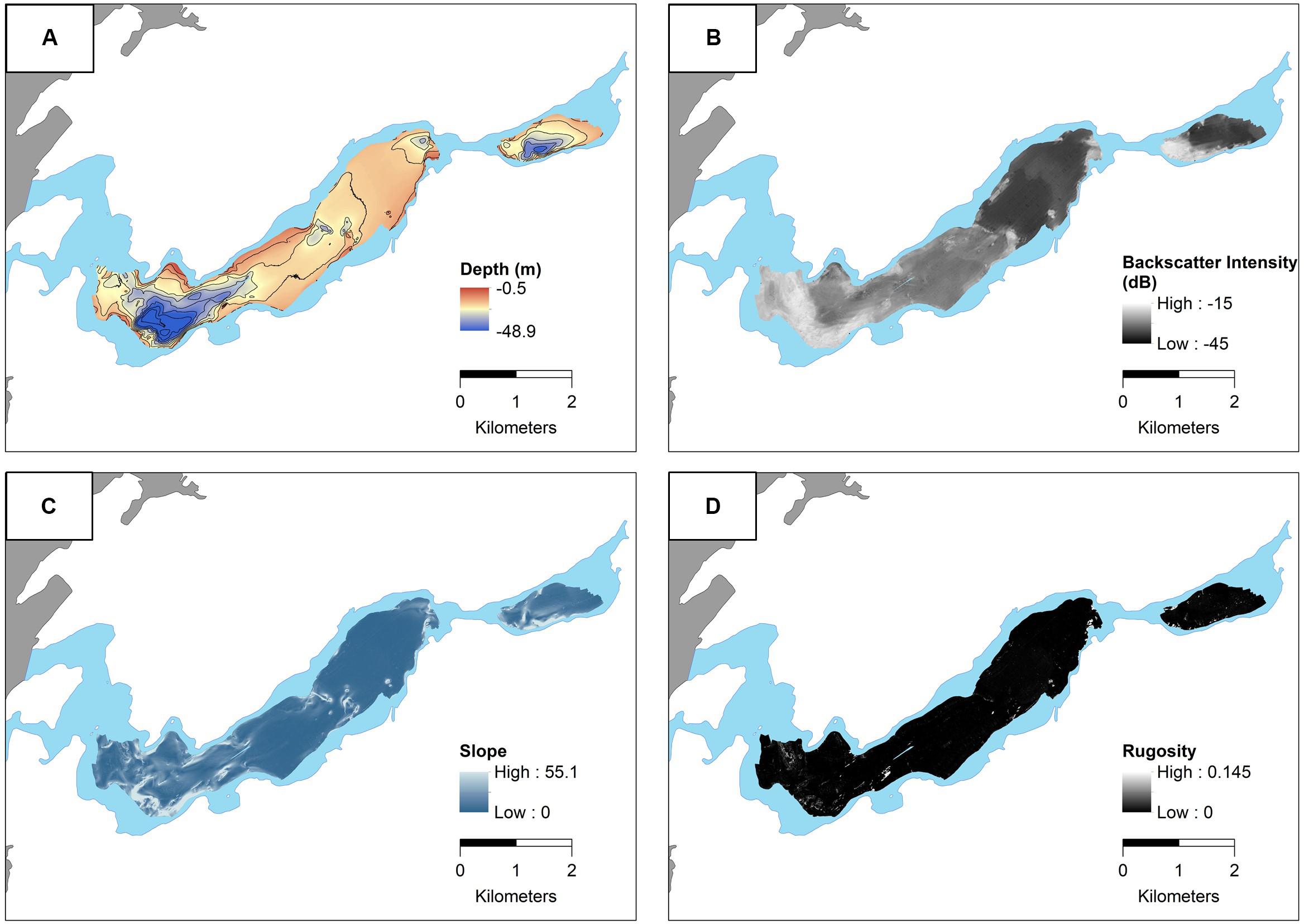
Figure 2. Results from the 2017 Kongsberg EM3002D MBES survey of Loch Creran showing (A) bathymetry data (corrected to Lowest Astronomical Tide), and (B) backscatter intensity (dB); (C) slope and (D) rugosity were derived from the bathymetry data during data processing. The rasters shown have been merged and resampled to 2 m resolution. Prior to classification using Iso-cluster, the data were normalised to a scale between 0 and 1.

Classifying MBES data using clustering algorithms is a common technique used in benthic habitat mapping, however, there is presently no standardised method for this process (Calvert et al., 2015; Diesing and Stephens, 2015). A true UIC approach segregates groups of shared spatial properties between the unlabelled input variables into an optimised number of classes, and does not require prior knowledge of the seabed (Jain, 2010). However, the tool we used required a user-defined number to produce a signature file. Selecting the optimum number of classes is subject to uncertainty and can involve complex processing, decision-making (Ahmed and Demšar, 2013), and a good understanding of the study area. To aid this decision, the number of user-defined classes was thus optimised using the MLC Confidence output from the ArcGIS tool (Dove et al., 2014) in combination with the results from the classification of video survey images. The UIC tool is a clustering algorithm that arranges the input data and identifies the most likely clusters based on the user-defined number to produce a signature file. The MLC confidence output calculates the number of cells that have a probability of being correctly assigned to a class over 14 confidence levels. Level 1 has a 100% probability of the cells being assigned correctly. This output was tested for five different user-defined classes ranging from 5 to 9, using the output from the image classification to provide a sensible starting point. The number of classes with the highest number of cells at 100% confidence was 7 (see Supplementary Table 1). This agreed with the estimated number of sediment types observed during the classification of video survey images (see section “Sediment Folk Classification”).

Grab Sampling

We used the resulting classification from “Pre-sampling: Classification of MBES Data (Sampling Strategy)” to determine the spatial locations for the ground-truthing samples. The goal was to collect grab material from every class whilst avoiding the protected features (Figure 1). We collected 28 grab samples over two research cruises, in May 2018 and August 2018 (Figure 3 and Supplementary Table 2); consent was granted by Scottish Natural Heritage for sampling within a Marine Protected Area (MPA). Sediment samples were collected using a hand-held Van Veen grab (0.01 m²), penetrating up to 10 cm depth. The GPS position and depth of samples were recorded from the research vessel, RV Morwena, at the point of contact with the seabed. The grab was emptied into a collection box and a representative scoop (approximately 300 g) across the full depth of the bulk sediment was collected. Samples were refrigerated at 4°C on return to the lab, pending analysis.

FIGURE 3

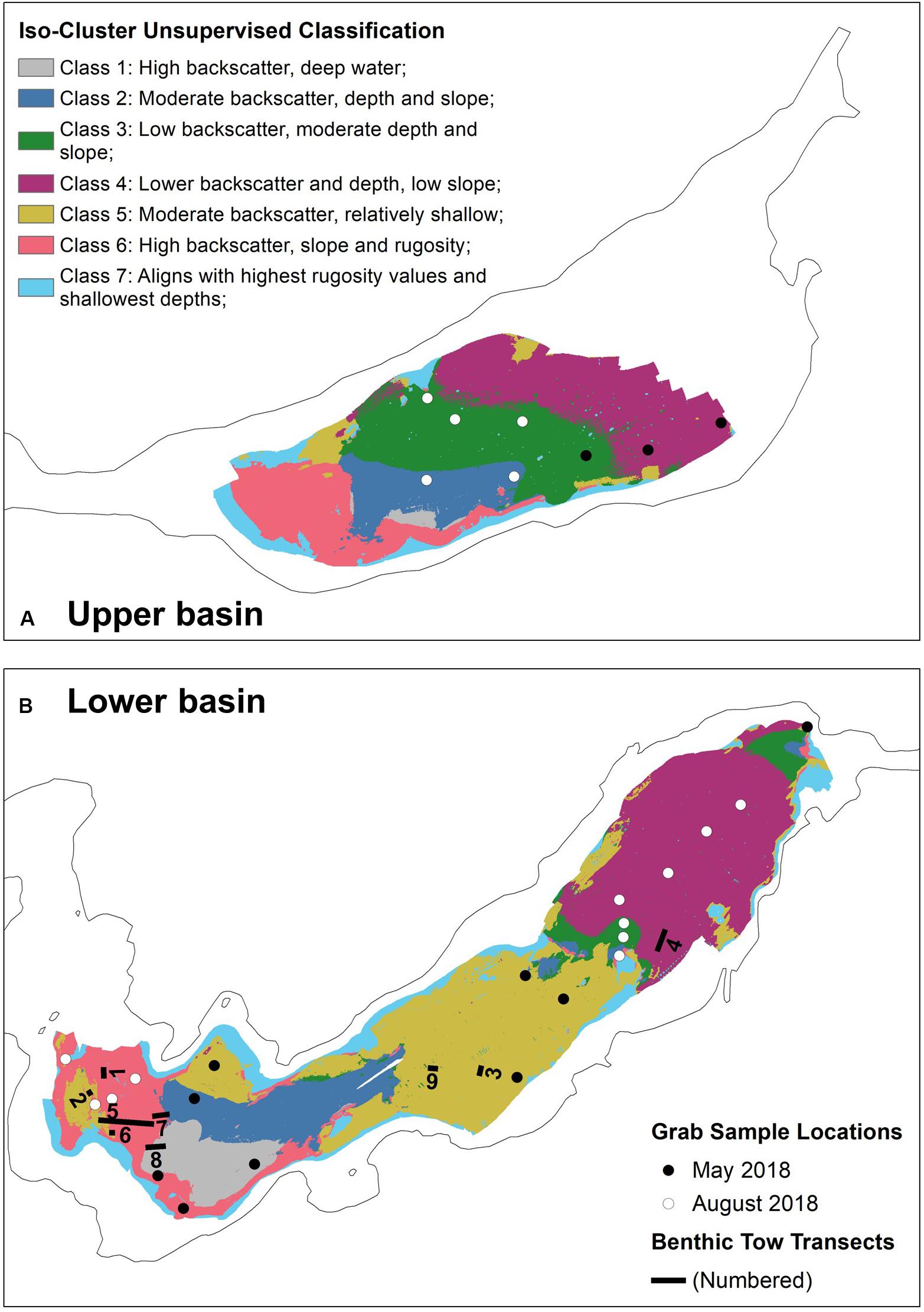
Figure 3. Classified maps of Loch Creran split into (A) Upper basin and (B) Lower basin, using Unsupervised Iso-Cluster tool, showing the ground-truth sample locations collected in May 2018 (black circles) and August 2018 (white circles). The benthic tow transects carried out in the Lower basin are shown as numbered solid black lines.

At each grab sample location, a corresponding value for each of the raster inputs (bathymetry, backscatter, rugosity and slope) was extracted using Focal Statistics (circular nearest neighbour approach, 3 × 3). A qualitative description was generated for each of the classes based on characteristics of the MBES raster data (Figure 4).

FIGURE 4

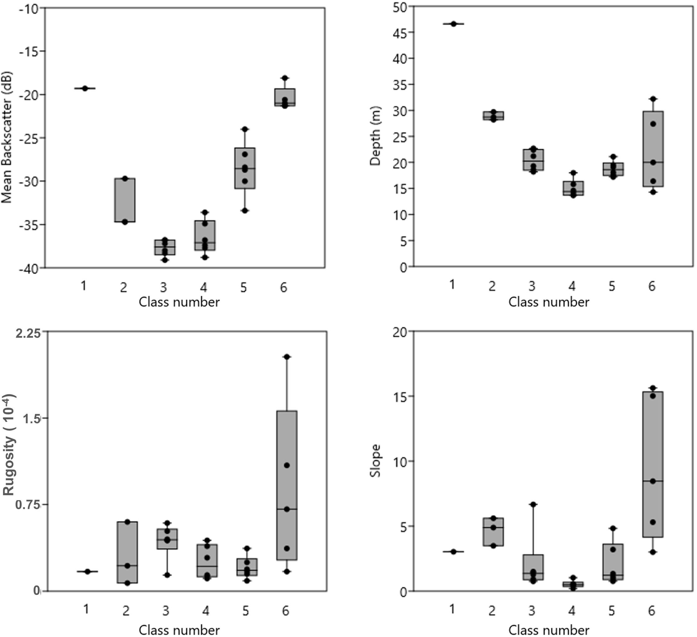
Figure 4. Boxplots showing the pre-normalised values of the MBES parameters used in the Unsupervised Iso-cluster Classification. Individual grab samples have been grouped by class.

Sediment Properties Analyses

We analysed the physical and geochemical properties of the sediment from each grab sample as described in the following sub-sections. The results are summarised in Tables 1, 2.

TABLE 1

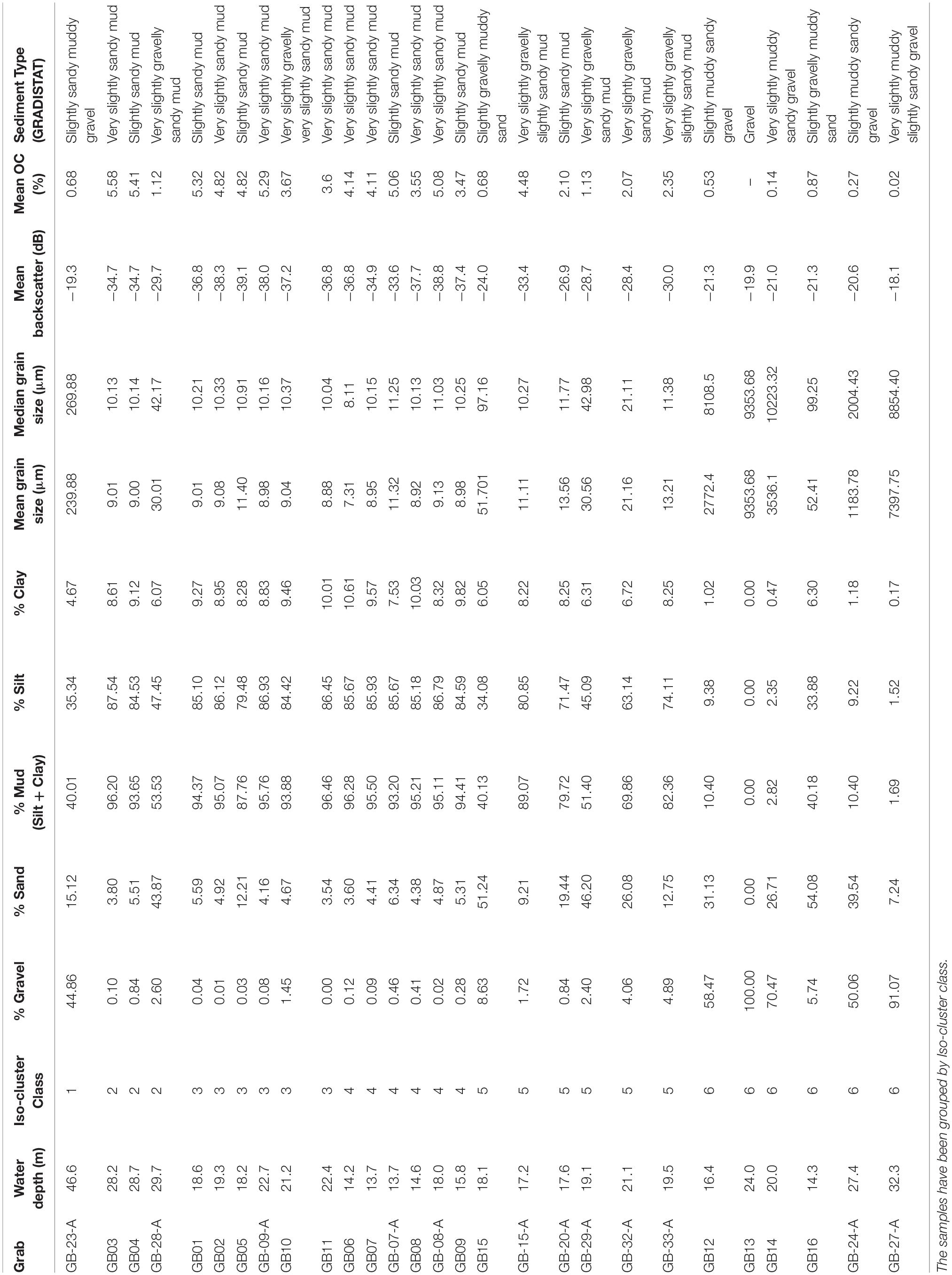
Table 1. Loch Creran sediment composition and grain size statistics for each grab sample as calculated by GRADISTAT; mean backscatter intensity (dB) and OC% values are also included for each sample.

TABLE 2

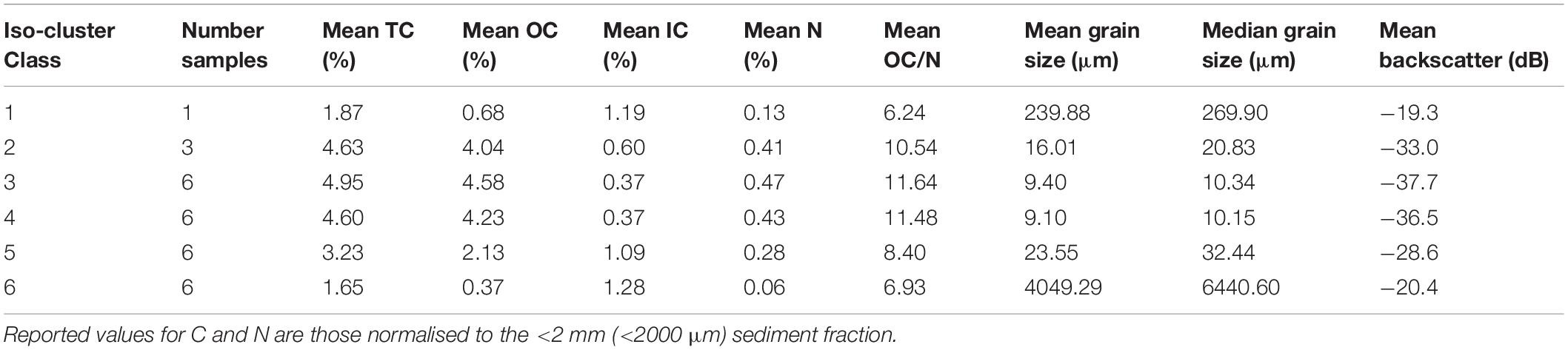
Table 2. Summary of elemental and physical properties for each class from Loch Creran derived by averaging the results from all grab samples within each class.

Carbon and Nitrogen Analysis

Approximately 40 g of material was removed from the homogenised bulk sediment and freeze-dried. The sedimentary OC, total C, and total nitrogen (N) content was measured using an ‘Elementar EL Vario’ Elemental Analyzer. Based on the method from Verardo et al. (1990), all samples were milled into a homogenous powder, except for the contents of grab GB13 which were too coarse for elemental analysis. 10 ± 0.1 mg was subsampled from the fine matrix (<2000 μm) and measured into tin capsules for analysis of total carbon (TC) and N. For OC, another 10 ± 0.1 mg of sample was measured into silver capsules and subsequently acidified with 10% HCl to remove the carbonate material. These capsules were dried overnight at 60°C prior to analysis. The inorganic carbon (IC) content was derived as the difference between TC and OC. The analytical precision of the method was calculated through repeat measurements of a standard reference material, B2178 (Medium Organic Content Standard; Elemental Microanalysis, United Kingdom) which yielded results for C = 0.06% and N = 0.05% (n = 18). The OC/N ratios presented have been normalized to the molar mass (C = 12 g/mol; N = 14 g/mol) using the unacidified nitrogen values (Kennedy et al., 2005), i.e., total N. The resulting OC values were normalised to the <2000 μm sediment fraction following the particle sizing to represent the sediment fraction that was analyzed for OC content and allow for better comparison across the mixed sediments.

Particle Size Distribution

To characterise the sediment composition for each grab sample, a method adapted from Blott et al. (2004) was used to analyse the fine fractions, before merging with the coarse fraction (Mason, 2011) into a full particle size distribution.

Fine fraction (<2000 μm) volumetric analysis

Laser granulometry (Coulter-Beckman LS230) was used to measure the volumetric proportion of the fractions between 0.3 μm – 2000 μm. Due to the high levels of OM within fjordic sediments we compared the particle size results from samples that had been pre-treated with 30% hydrogen peroxide (H₂O₂) and 10% hydrochloric acid (HCl) to remove the OM and carbonate material, against untreated samples. We found that the high levels of OM in the untreated samples masked the presence of sands (clearly visible in some samples) within the sediment and generated misleading results by skewing toward the fine fractions only (Hayton et al., 2001). We have thus consciously chosen to use the pre-treated laser results which give a better representation of the <2000 μm sediment fraction for these samples.

Coarse (>2000 μm) and fine fraction (<2000 μm) weight analysis

The remaining sample, typically between 200 g and 300 g of sediment, was wet-sieved at 2 mm to separate the coarse and fine fractions. The remaining coarse fraction was washed into a container and dried until constant temperature at 60°C. Samples were then dry-sieved for 10 min through sieves at 1/2 phi intervals: 8, 5.4, 4, and 2 mm. The material collected on each sieve was weighed to 0.1 g. The fine fraction was left to fully settle in the collecting beaker before the overlying water was syphoned off. The settled material was dried at 60°C until constant weight.

Full particle size distribution

Volumetric proportions measured by the laser granulometer were converted to an equivalent weight-percentage using the total weight of the <2 mm fraction collected during sieving prior to merging with the sieve data (Mason, 2011). We grouped the millimetre-scale size data into phi classes using size class boundaries according to Blott and Pye (2001) (see Supplementary Table 4). Statistical parameters were calculated for each sample using the GRADISTAT software (Blott and Pye, 2001) (Table 1). We use the mean grain size of the samples to compare with the backscatter and geochemical data. Occasionally, terrestrial OM with a high surface area (e.g., leaf, root or woody material) was caught at the large sieve fraction, however, weighed very little. This is reflected in the full particle size distribution results where a gravel-size component is shown to be present, but with negligible weight (e.g., samples within class 2, 3, and 4).

Organic Carbon Spatial Prediction and Quantification

The basis for the spatial prediction for OC by backscatter was built on the evidence for empirical relationships between sediment grain size and OC (Hedges and Keil, 1995; Flemming and Delafontaine, 2000; Burdige, 2005; McBreen et al., 2008) and acoustic backscatter correlation with grain size (Goff et al., 2000; Collier and Brown, 2005; Serpetti et al., 2011). To enable a spatial prediction of OC content across the backscatter survey area, we performed a linear squares regression (Equation 1) (Python V3.2 ‘scipy.optimize.curve_fit function’) correlating the mean backscatter value for each grab sample location (see section “Grab Sampling”) and the normalised OC% value derived from elemental analysis. A comparison was made with a 2nd order polynomial regression (Equation 2) which yielded similar r² results (Table 3); thus, the simpler linear model was adopted. The equations for the line of best fit (Equation 1) and associated 95% confidence intervals (Equation 3) were applied to the backscatter raster using the ArcGIS Raster Calculator to spatially model OC% and its associated uncertainty for each backscatter value.

TABLE 3

Table 3. Comparison of linear regression results for mean backscatter (dB) and OC% data from Loch Creran surface sediments where y = OC%, x = backscatter intensity (dB).

To quantify the mass of OC within the surface sediment (top 10 cm), class-specific stocks based on volumetric and mass calculations were made following Burrows et al. (2017). Representative dry bulk density (DBD) values were calculated using core data collected from Loch Creran in 2016 and subsequently archived at the University of St Andrews. The cores were spatially correlated with our raster class areas and the DBD was derived by averaging the values from the top 10 cm pre-dried and weighed core slices (each slice = 1 cm). The DBD, which was related to the sediment type based on the output from GRADISTAT, was applied to the whole class area (Table 1). For those classes where there were no spatially co-located cores, typical DBD values for sediment types were obtained from the literature based on the GRADISAT classification for the relevant samples (Supplementary Table 5).

The total area of each class was calculated within ArcGIS. To derive a single mean percentage for OC and associated uncertainty for each class, we used the ArcGIS Zonal Statistics tool. OC stocks were determined assuming a standard depth of 0.1 m, using the steps shown in Supplementary Table 6.

Results

Loch Creran Physiography

The bathymetry data show good agreement with the general understanding of the topographic nature of Loch Creran (Black et al., 2000). There are two ‘deeps’, one in each basin located toward the south-western sides (Figure 2). The backscatter data show large-scale variation across Loch Creran implying sediment heterogeneity with the range of intensity falling mostly between −39 dB and −14 dB. Within each basin, similar transitional gradients are seen from the head (far east) to the mouth (far west), from large areas of dark, low intensity values, implying homogenous soft sediments, to higher intensity backscatter values representing higher variability from mixed substrate. The rugosity values show little variability within Loch Creran, although higher values implying seabed complexity are aligned with steeper slopes in the lower basin and on the periphery of the survey area in shallower waters. These areas correlate spatially with the Serpulid aggregations and Flame shell beds and previous side scan sonar work within Loch Creran has been shown to successfully identify these reef structures (Fournier et al., 2010).

MBES Iso-Cluster Classification and Ground-Truthing

The map of the MBES Iso-cluster classification is shown in Figure 3. As noted, seven classes were selected for having the highest number of cells predicted with 100% confidence from the Maximum Likelihood classification output (Supplementary Table 1); however, no sample data exist for class 7 due to proximity to protected features. The mean values of each input parameter, backscatter, bathymetry, rugosity, and slope, for each grab sample location indicate different characteristics associated with each class (Figure 4). Class 6 exhibits the highest backscatter values alongside large ranges for depth, rugosity and slope values potentially indicating an influence of different seabed characteristics on the backscatter signal.

Twenty eight grab samples (Table 1) were collected within classes 1–6; only one grab was collected successfully within class 1. Samples were not, however, collected from class 7 due to the proximity of these areas to protected features (Figure 1). Samples are grouped by classes for subsequent analyses to help identify whether our unsupervised classification method was able to discriminate different sediment types. This tells us whether the ground truth samples collected are generally representative of the sediment types found within Loch Creran. However, it is important to clarify that the individual sample data independent of the classification groupings are considered because one aim of this study is to investigate the relationships between sediment grainsize, backscatter and OC content. There was good agreement between bathymetric depths derived from the MBES survey and those recorded by the sampling vessel’s echosounder at each grab sample location, with mean divergence of 1.5 m and standard deviation divergence also of 1.5 m for 28 sample pair differences. Possible sources of difference may have resulted from boat drift, tidal range, and/or currents within the sea-loch moving the grab assembly while lowered below the vessel.

Sediment Folk Classification

In total, 980 seabed sediment images were visually classified using a simplified Folk Scheme (described in Long, 2006). The images showed clear heterogeneity of sediment types within Loch Creran (Figure 5). We used the images to relate the backscatter signal to a predicted sediment type. As predicted, the transects taken over ‘darker’ (i.e., lower values) areas on the backscatter map (T9 and T3) are characterised by homogenous muddy sediments, with little observed macro-benthos. Transects appearing to cross substrate transition zones show the highest heterogeneity in sediment type, with a higher gravel component (larger clasts were identified using the 10 cm laser for scale), implying higher energy environments. Using this method, we identified up to seven possible sediment types and used these to inform the required user-input of classes (see Supplementary Table 1) for UIC. While the video transects do not overlap directly with our ground-truthing locations (Figure 3), we believe that the images provide a useful ground-truthing component for interpreting the MBES backscatter results prior to sampling. Video transects have the advantage of covering large areas of seabed compared to grab samples within the same survey period.

FIGURE 5

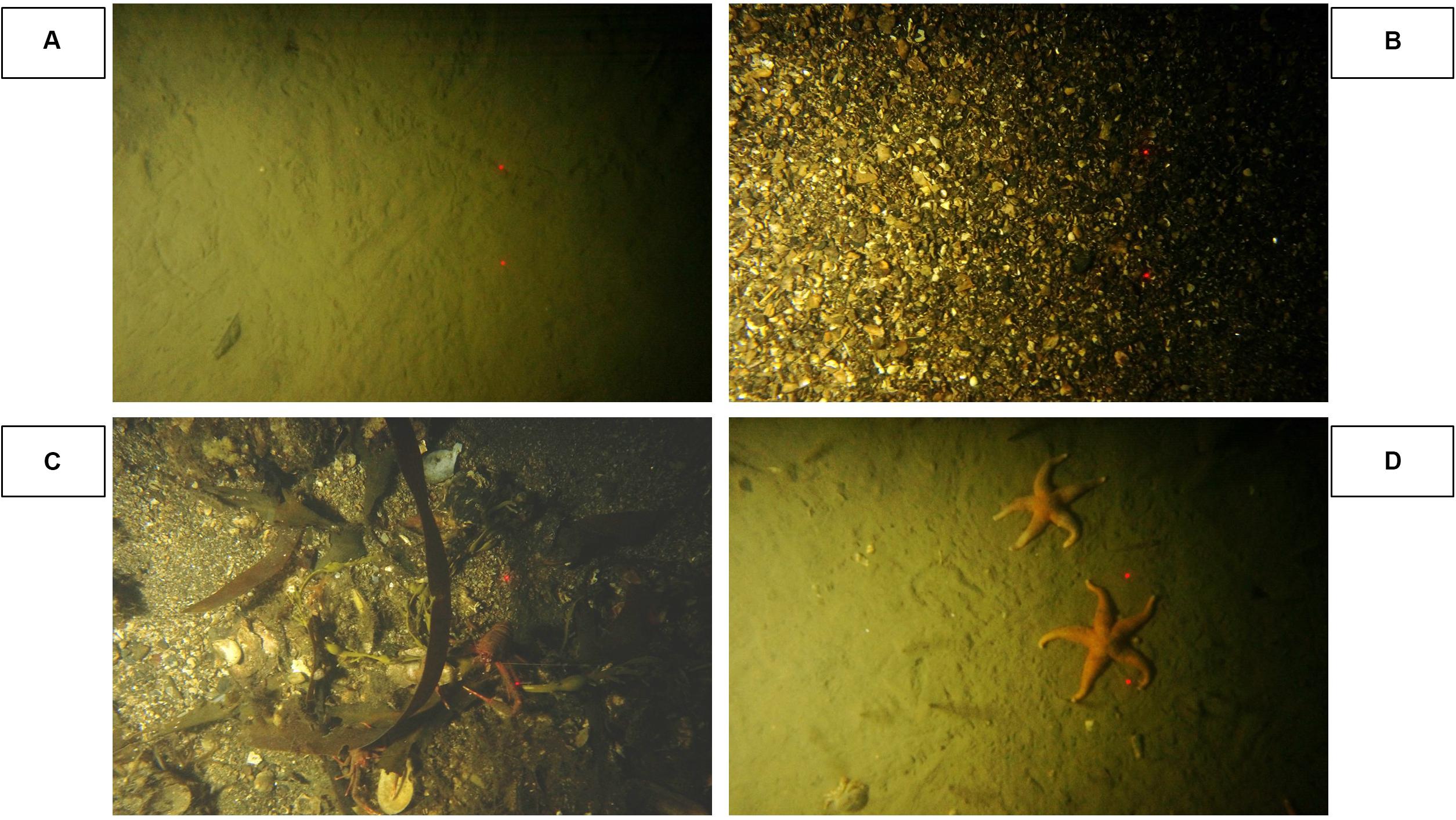
Figure 5. (A–D) Example Loch Creran seabed images collected by the BGS benthic tow fish. Sediment types were classified using a simplified Folk Scheme, thus: (A) T4 – Mud (M); (B) T6 – Gravel (G); (C) T1 – gravelly Sand (gS); (D) T3 – sandy Mud (sM). Spatial locations of the benthic tow transects (T1–T9) are shown in Figure 3B. Red dots represent 10 cm laser spot separation for scale.

Particle Size Distribution

We analysed the combined particle size data using GRADISTAT (Blott and Pye, 2001) to derive grain size statistics for each sample (Table 1). The GRADISTAT results demonstrate spatial variation in the mean and median grain sizes of sediment supporting the acoustic and video evidence of a heterogeneous seabed within Loch Creran. A Pearson correlation (r = 0.6) and corresponding p-value (0.0012) indicate a statistically significant correlation between mean backscatter and grainsize within our samples. Specifically, areas of low backscatter intensity (∼−35 dB) are characterised by low mean sediment grain sizes (∼10 μm) with high proportions of silt (Table 1). These sediments are described texturally as variants of ‘Slightly Gravelly Mud’ (Folk, 1954) with gravel contents < 1%, apart from GB10 and GB-28-A which have a slightly higher gravel content at 1.45 and 2.60% respectively. High backscatter areas (>−25 dB) are characterised by highly variable mean grainsizes that range from as low as ∼50 μm up to the maximum observed mean value of 9.4 mm.

To assess the effectiveness of the unsupervised clustering routine in differentiating sediment types, we plotted the bulk sediment compositions from grab samples on a ternary diagram (Blott and Pye, 2012) (Figure 6). The samples were grouped by iso-cluster class to identify patterns and/or variability within each class. Three broad sediment groups are illustrated: mud to muddy sand (classes 2, 3, 4, and 5); muddy gravel (class 1) and a coarser sandy gravel to gravel (class 6). There are two class outliers; the first is sample GB-28-A in class 2 which has a rugosity value (7 × 10^–6) an order of magnitude smaller than GB03 and GB04 (2.2 × 10^–5 and 6 × 10^–5 respectively) but a higher backscatter value of −29.7 dB compared to −34.7 dB. The increase in backscatter intensity could be explained by the higher proportion of coarse material (2.6% gravel and 43.9% sand) compared to GB03 and GB04. The second outlier from class 6, GB16, is characterised as a slightly muddy gravelly sand. The sample falls very close to the class 5/class 6 boundary to the furthest western side of the MBES survey area and has a similar sediment composition to the other samples from class 5; however, the sample exhibits a backscatter, rugosity and slope value similar to those samples in class 6 (Figure 4). Sediments in classes 2, 3, and 4 exhibit a gradual shift from mud to sandy mud. There is greater variability in the sediment textures of samples in classes 5 and 6 which are composed of the coarser sediment types. It is interesting to note that those coarser samples with a higher mud content (combined particles within the clay and silt fractions) exhibit higher OC contents; GB-15-A and GB-33-A have a mud content and OC content of 89.1% and 4.55% and 82.3% and 2.47% respectively (Table 1 and Supplementary Table 7). The variability within these classes implies that there will be higher uncertainty in any C values associated with these areas due to greater sample heterogeneity.

FIGURE 6

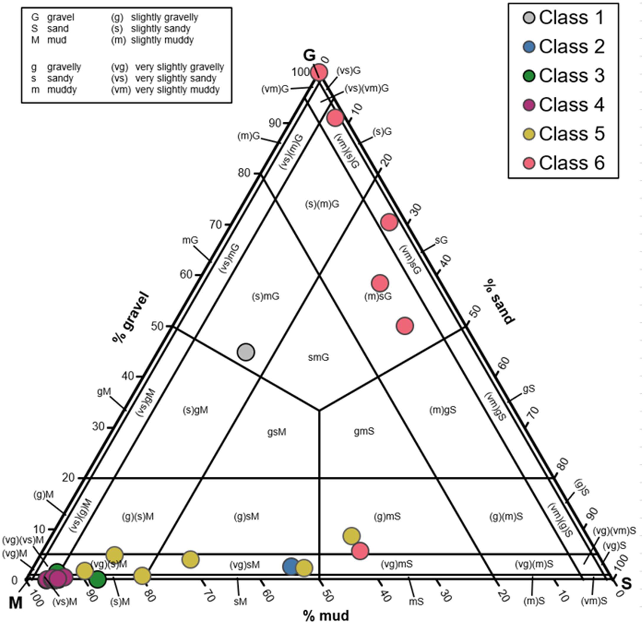
Figure 6. Loch Creran particle size results plotted on a ternary diagram based on the proportion of gravel, sand and mud fractions (Blott and Pye, 2012). Individual samples are grouped by colour into classes based on the Unsupervised Iso-cluster Classification.

To investigate the particle size distributions between grabs, sediments were grouped into major fractions (Figure 7) following suggested size boundaries by Blott and Pye (2001) (Supplementary Table 4). Grain size frequency histograms of the samples show variability in the sediment composition between the classes. Classes 1 and 6 have considerably different mean grainsize distribution patterns from the other classes. Meanwhile, classes 2, 3, and 4 exhibit similar mean composite patterns, although there is greater variability between individual grabs within class 2. This may be due to the fact there are fewer samples within this class, one of which has a higher proportion of sand and is an outlier (GB-28-A), mentioned previously. Classes 3 and 4 are very similar displaying low variability between individual samples. This suggests that the sediments found within these classes are homogenous in composition; the difference in depth between these classes is the likely reason that they cluster separately (Figures 2A, 4).

FIGURE 7

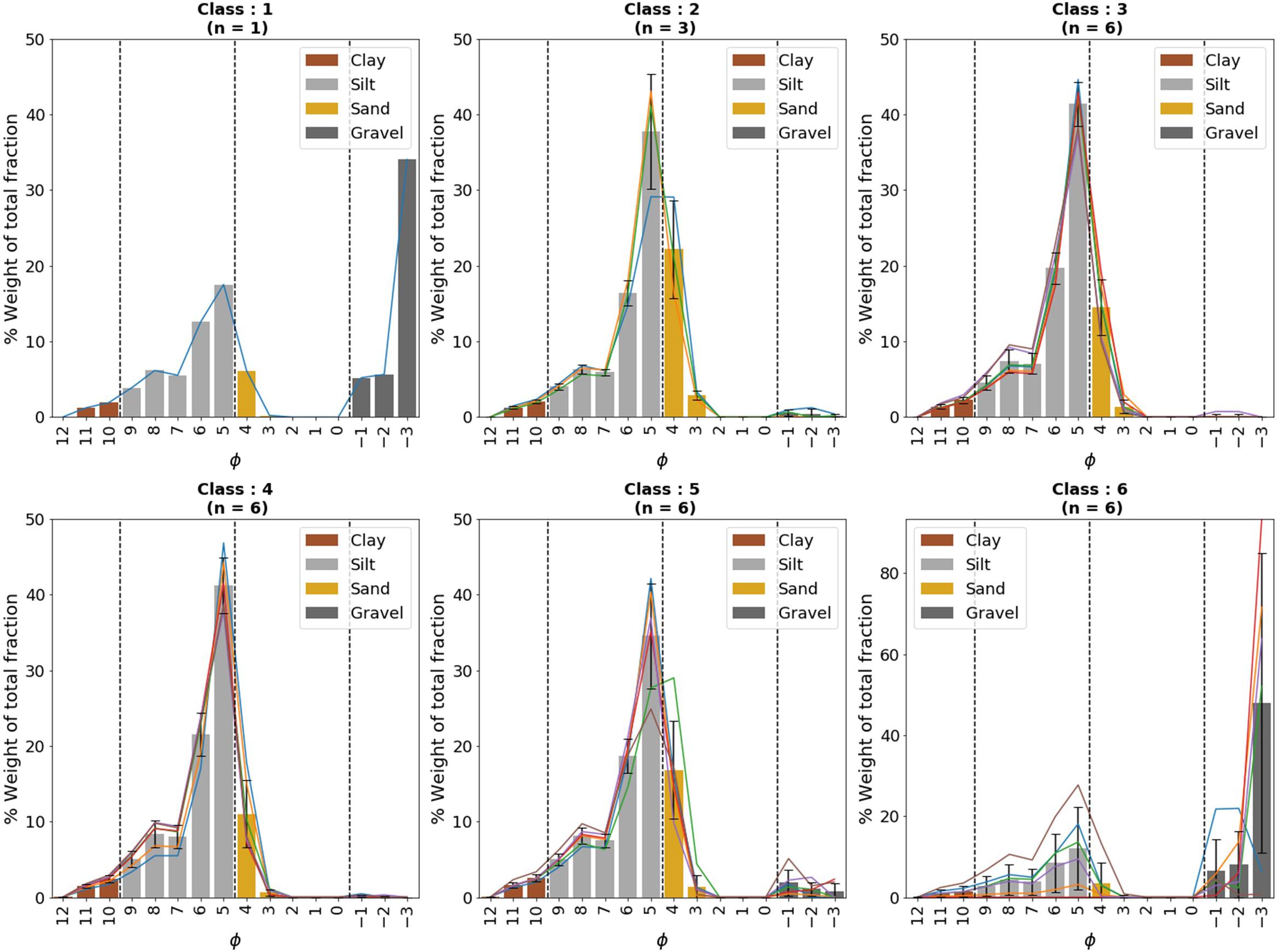
Figure 7. Loch Creran sediment particle size distributions converted to phi scale for each class output from the Unsupervised Iso-cluster Classification. For each class, the continuous lines show the grain size results for individual samples and the frequency histograms show the composite mean results at the individual size fractions for the combined number of grab samples (n). Error bars show the standard deviation at each size fraction to highlight variability. Bar colours and dashed vertical lines differentiate the proportions of clay (>9 φ) or (<2 μm), silt (8 φ – 5 φ) or (2 μm – 63 μm), sand (4 φ – 0 φ) or (63 μm – 2000 μm) and gravel (<0 φ) or (>2000 μm). Note that the φ scale has been inverted and larger grain size plot to the right. Class 6 has a different scale on the y-axis.

The sole sample from class 1 is made up of an even proportion of clay, silt, sand (combined < 20%) and a large gravel component. Considering the coarseness of this sample (mean grain size of 240 μm), a relatively high OC content of 1.23% is reported, suggesting that the proportion of fine particles may control the presence of OC. Classes 2, 3, 4, and 5 are largely composed of silt fractions, with higher fractions of sand seen in classes 2 and 5. Class 6 sediments are shown to be generally coarse with samples having over 50% of the sediment > 2 mm and very small fractions of clay, silt and OC.

Carbon and Nitrogen Analysis

Results are shown grouped by class in Table 2; individual sample results can be found in the Supplementary Table 7. Our results show a spatial distinction in the characteristics of the bulk C and N values held in Loch Creran’s surface sediments and between the different classes. The highest values of OC are found within the fine-grained sediments toward the head of the fjord. A decline is seen seawards with the lowest OC values in areas of coarse sediments closer to the mouth. Sample OC% values range from 5.58% (class 3, upper basin) to 0.02% (class 6, lower basin). Classes 2, 3, and 4 are enriched in OC (>4%) compared to classes 1, 5, and 6 which have mean OC% values (<2%) below the sample mean value of 2.98%. Total nitrogen (N)% content and OC/N ratios of the samples follow a similar pattern so that OC rich sediments are also relatively enriched in nitrogen. A strong correlation between N and OC is seen (r² = 0.92) which can be indicative of a common (organic) source (Goñi et al., 2013; Faust and Knies, 2019). N% ranges from 0.66% to 0.01% with a mean value of 0.32%. OC/N ratios can be used to infer the source of OM, although must be interpreted cautiously in isolation because degradation processes can alter the ratios from that of the source material (Thornton and McManus, 1994; Bianchi and Canuel, 2011). Nonetheless, we see spatial heterogeneity in the OC/N ratios of our samples. The average OC/N for samples is 9.69; the values range from 6.24 to 13.72 indicating a mixture of sources potentially similar to those identified in Smeaton and Austin’s study (Smeaton and Austin, 2017) from a nearby fjord (e.g., phytoplankton, macroalgae and terrestrial soils/leaf matter). A spatial analysis of the OC/N values indicates sediments at the seaward end of the loch receive marine-dominated sources of organic material compared to the inner regions (Smeaton and Austin, 2017). Relatively lower OC/N values are seen in samples with relatively higher proportions of IC (Table 2 and Supplementary Table 7).

Combined Physical and Geochemical Properties

As expected, based on empirical relationships between backscatter, mean grainsize, and OC, we observe trends between these variables (Figure 8). Overall, there is a stronger correlation for both OC and backscatter at grain sizes up to 100 μm, after which the predictive power of the model decreases with larger mean grain size (see correlation equations and associated r² values in the caption of Figure 8).

FIGURE 8

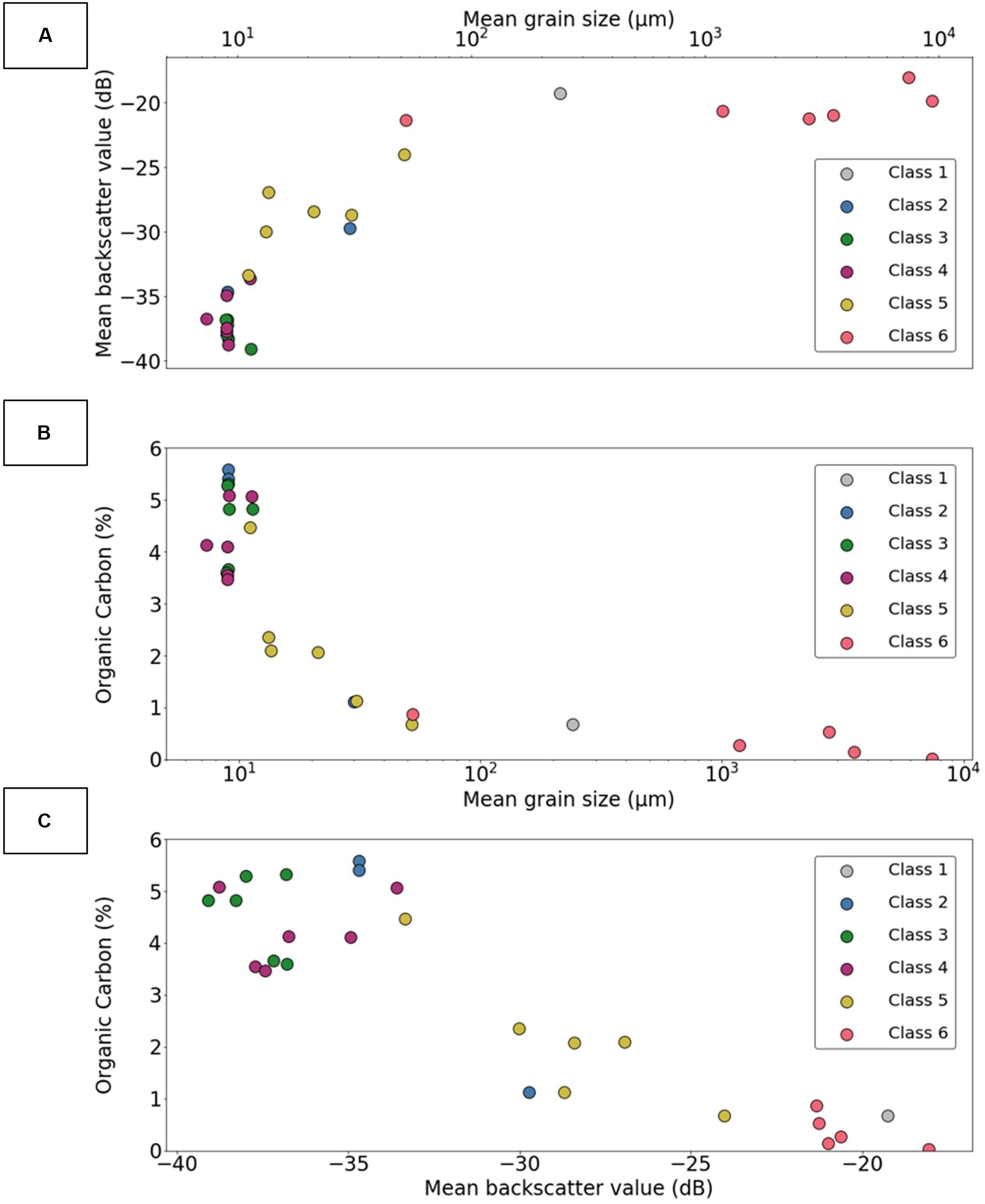
Figure 8. Scatterplots showing the relationships between (A) mean grain size, x (μm) and mean backscatter intensity, y (dB) [logarithmic; y=2.68 ln(x); r² = 0.74], (B) mean grain size, x (μm) and organic carbon content, y (%) (power; y=15.02x^{– 0.6}; r² = 0.87) and (C) organic carbon content, y (%) and mean backscatter intensity, x (dB) (linear; –y = –0.2506x–4.797; r² = 0.82) for each grab sample from Loch Creran.

A positive correlation is observed between mean grain size and backscatter intensity (r² = 0.74) (Figure 8A). A cluster of samples from classes 2, 3, and 4 have a similar mean grain size of 10 μm but have considerable backscatter variation (a range of ∼5 dB) suggesting that small differences in surface sediment composition can have a large impact on scatter. The highest backscatter values (>−22 dB) are seen for sediments with a larger mean grain size (10² – 10⁴ μm). There is a negative correlation between the mean grain size and the OC content of the sediment (Figure 8B). The clustering pattern, seen in Figure 8A for mean grain sizes of approximately 10 μm, is again observed, with variability in the amounts of OC. Fine sediments (<10² μm) are relatively enriched with OC as we might expect and a strong exponential relationship is seen specifically between OC% and % mud fraction (r² = 0.88) from our samples (Supplementary Table 7). Finally, a negative, linear correlation (r² = 0.82) is observed between OC content and backscatter intensity (Figures 8C, 9). Based on the observations above, finer-grained sediments exert a stronger control on OC% and have a relatively lower backscatter intensity. As grainsize increases, so does backscatter intensity, however, due to the disproportionate effect of gravel on backscatter (Goff et al., 2000), the ability to predict OC% diminishes. Nonetheless, these relationships enable us to use backscatter intensity as a means for identifying spatial distributions in surficial OM on the seabed.

FIGURE 9

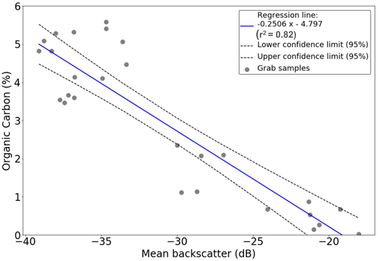
Figure 9. Results of linear regression correlating mean backscatter with OC for each grab sample from Loch Creran; 95% confidence intervals are displayed.

Organic Carbon Spatial Assessment and Quantification

As described in Section “Organic Carbon Spatial Prediction and Quantification” regression models were performed to describe the relationship between backscatter intensity and OC% and are shown in Table 3. The linear model (Figure 9) was selected for its simplicity over the 2nd order polynomial fit, which does not provide additional explanatory power. The coefficients of the linear regression were applied to the backscatter raster (merged, and re-sampled to 2 m) using the ArcGIS Raster Calculator to generate spatially explicit predicted values for OC% for each backscatter value (Figure 10); spatially predicted 95% confidence limits for each backscatter value were also generated using the following equation (Equation 3):

FIGURE 10

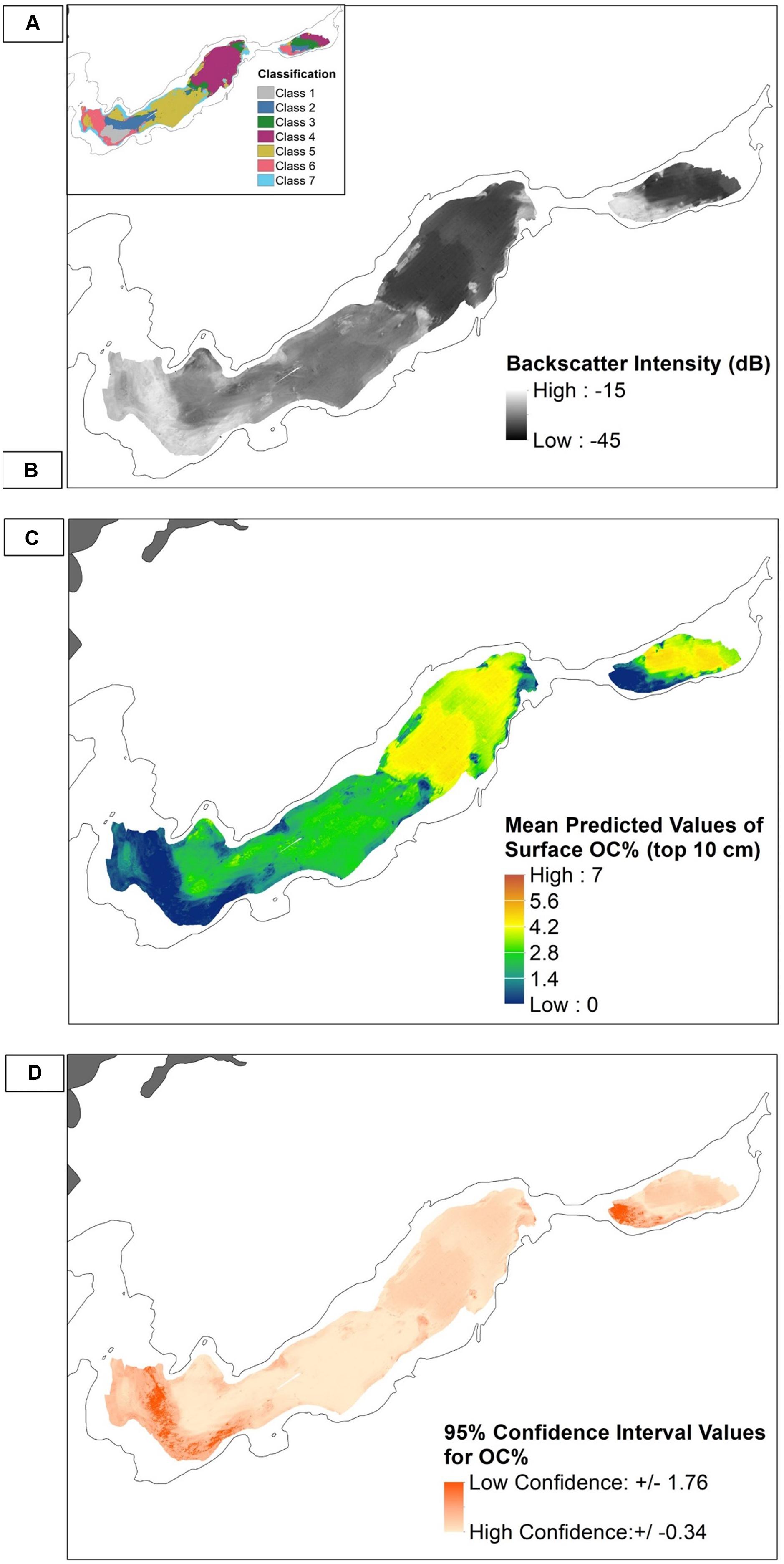
Figure 10. Loch Creran surface sediments; (A) Iso-cluster Classified areas; (B) Backscatter (dB) results from MBES survey, (C) Spatially predicted map of OC% based on the linear regression correlation found between backscatter and OC% and (D) Spatial map of confidence intervals for predicted OC% values.

95 % c o n f i d e n c e i n t e r v a l = t \times \sqrt{\frac{S_{e r r}}{n - 2} \times \frac{1}{n} + (\frac{{(x - m e a n_{d f})}^{2}}{\sum (d f^{2}) - n \times (m e a n_{d f}^{2})})}

where t is the standard t value for a two-tailed test, n is the number of grab samples, S_err is the sum of the square of the residuals, mean_df is the mean backscatter value from the grab samples, $\sum (d f^{2})$ is sum of backscatter values squared, and x is the backscatter pixel value. Using these results, spatially predicted OC% values across the MBES survey area with upper and lower confidence intervals were derived. The modeled spatial pattern for the OC% content within Loch Creran follows that of the acoustic backscatter data. The highest predicted OC values, those >4%, are seen within classes 3 and 4, coincident with the lower intensity backscatter values and finer sediments. The 95% confidence intervals range from 0.3% to 0.5% throughout Loch Creran, however, higher values ∼ >1.0% are seen in small regions of class 6, concurrent with the lowest predicted levels of OC and coarsest sediments. Surface stocks of OC were calculated for both the MBES survey area (60% of area) and total seabed area of Loch Creran as detailed in Section “Organic Carbon Spatial Prediction and Quantification” with results shown in Table 4; for the total seabed area of Loch Creran, we estimate a total surface (10 cm) stock of 20,577 ± 4,462 t. To assess the robustness of this estimate we compared our result against that of Smeaton et al. (2017), who estimated a total volumetric mass of 3.0 ± 0.5 Mt of OC for Loch Creran, based on a seismically modeled mean post-glacial sediment depth of 13 m. When directly scaled down to a 10 cm depth, this yields an estimated stock of 23,077 ± 3,846 t OC. This comparison assumes an even distribution of OC throughout the total sediment column which is a more likely scenario below an average burial depth of 30 – 50 cm (Johannessen and Macdonald, 2016), but we recognise that surface sedimentary OC is actively cycled due to the likes of resuspension events (Almroth-Rosell et al., 2012) and remineralisation by benthic organisms and therefore likely to be much more variable. Nevertheless, our estimate including uncertainty compares very reasonably with Smeaton et al. (2017) despite the different approaches.

TABLE 4

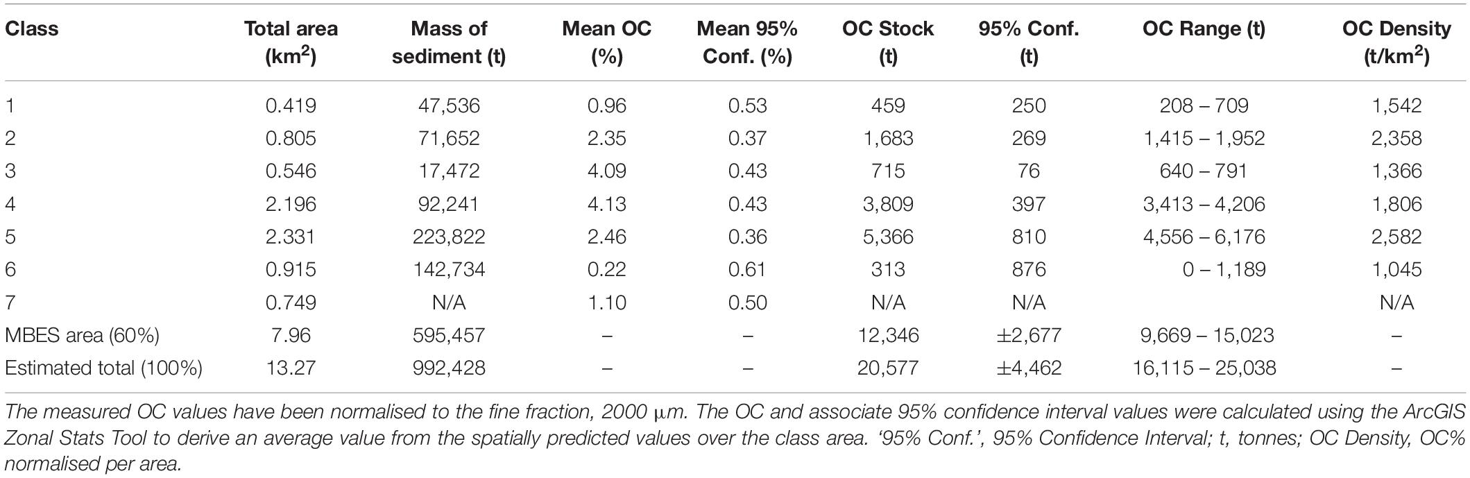
Table 4. Mass of sediment and the calculated mass of OC held within each class for the top 10 cm from Loch Creran using sediment specific DBD values.

Despite having lower average OC values, class 5 sediments hold the most OC through virtue of covering the largest area. However, to understand the effect of sediment type on the OC density, we have normalised the class stocks of OC by area (Table 4). We find that classes 3 and 4, composed of homogenous fine muddy sediments have a lower OC density than the mixed sediment classes, comprised of coarser silts and fine sands. This ‘phenomenon’ whereby the sediments hosting larger proportions of OC do not contribute to the highest OC stocks by area, results from the inclusion of bulk density values in the stock calculation (Flemming and Delafontaine, 2000; Burrows et al., 2017).

Discussion: a Novel Method for Mapping Sedimentary OC

The main aims of this study were two-fold; firstly, to assess the potential use of backscatter data as a proxy for OC and in doing so, to develop a novel methodology using MBES data to improve the spatial mapping of the OC component of surficial seabed sediments. Given the general paucity of high resolution data for sedimentary OC, this method could be used to supplement physical sediment samples and work toward improving national marine C accounting frameworks, for maritime nations (Avelar et al., 2017). Additionally, there is potential to overlay C-rich sediment maps with areas of human activities, for instance aggregate dredging, cable laying and benthic trawling, to assess the threat of disturbance to these carbon stores (Van De Velde et al., 2018).

Using Backscatter and Sediment Type as a Proxy for Organic Carbon in Loch Creran

Our study area is well-suited to test our hypothesis that acoustic backscatter data (highlighting a range of sediment types) may be used as a proxy for OC. The restricted geomorphology and relatively small area limiting the variability of inputs and flows within the system, OC-enriched sediments (Loh et al., 2008, 2010) and ease of sampling access has allowed us to test these relationships. Our results show a strong negative linear correlation (r² = 0.82) between mean backscatter and OC based on surficial sediments collected from the fjord. Using this relationship, we have produced a high-resolution spatial map of sedimentary OC with a bin size of 2 × 2 m. In addition, using spatially representative dry bulk densities, we estimate the surface standing stock of OC over the MBES area to be 12,346 ± 2,677 tones OC for the top 10 cm. While the integration of MBES, video and ground-truth data is commonly used within benthic habitat mapping studies (De Falco et al., 2010; Haris et al., 2012; Brown et al., 2019) here we extend this idea to develop a novel methodology to map the spatial variability of OC.

This study is complimentary to research carried out by Serpetti et al. (2012), who used a single beam echosounder device to map OM in a shelf environment on the east coast of Scotland. Their work first highlighted the potential of the application of acoustic reflectance data for mapping OC. Since, the development of acoustic technologies to the more commonly used MBES systems for seabed mapping and arguably a need for improved C-stock assessments, provides the rationale for developing this approach. Our results are in broad agreement with those of the previous study; we predict the highest values of OC to be in areas with low (relative) backscatter, coincident with homogenous fine-grained sediments. Our predicted uncertainty values are generally consistent (∼ ± 20% of the predicted OC value) across the survey area, however, these increase considerably in small areas characterised by high backscatter and coarse sediments, as seen by the weaker relationships with grain size >10² μm (Figure 8). We thus have lower confidence in the predicted OC values in these areas where the range of error is greater than the estimated value. However, values of OC are likely to be low in very coarse substrates as demonstrated by our results (Table 1). These localities experience high current flow (bed shear stress) as water is channelled through narrow passageways between the upper and lower basins and out into Loch Linnhe (Figure 1) and we would expect minimal deposition here (Black et al., 2000).

There are several factors to consider when interpreting backscatter data. Our results show a linear negative correlation between backscatter and OC (Figure 9) which is intrinsically linked to sediment grain size, although we do not see an entirely like-for-like relationship when compared to that of grain size and backscatter (Figure 8A). This may be due to the lower number of samples that were collected from coarser sediments or the volume of sediment collected for these more variable sediment types. Through the breakdown of sediment samples into their particle size distributions (Figure 7), we see that backscatter could be affected disproportionately by small amounts of coarse material (Goff et al., 2000; Diesing et al., 2014) – for example, grab samples from classes 2 and 5 have relatively low percentages of gravel although this translates into increased variability within each size fraction (see error bars within Figure 7) and a higher average backscatter signal for the class (Table 2). This effect is also seen within fine, well-sorted sediments having small percentages of sand such as those found within classes 3 and 4, whereby we see scatter variability for samples with the same mean grain size of ∼10 μm (Figure 8A). Acoustic discrimination of very fine sediments presents a challenge within current backscatter methods although use of a Bayesian statistical approach to unsupervised classifications has shown success in discriminating between homogenous areas (Alevizos et al., 2015). Processing developments in MBES data therefore provide opportunities for improved characterisation of the seabed.

As noted, we have observed clustering of samples for both backscatter intensity and OC% at a mean grain size of 10 μm. Ten μm is a notable size fraction in sedimentary science with sediments below this size demonstrating increasing cohesivity and reduced sensitivity to hydrodynamic sorting (McCave et al., 1995), which could explain this scattering effect. Above 10 μm, we can see the effect of increasing grain size more clearly on backscatter. The cohesive nature of fine silty sediments may help to explain why we see organic enrichment in sediments within Loch Creran despite regular flushing creating well-oxygenated waters (Black et al., 2000), combined with higher inputs of terrestrial material understood to be more refractory (Bianchi, 2011; Smeaton and Austin, 2017). Sedimentation rate may also have a control on OC content and burial rate at our site. Loch Creran experiences higher mass accumulation rates calculated from sediment trap data in the upper basin (11.11 g m² d) than the lower basin (4.42 g m² d) (Loh et al., 2010), which manifests in higher OC values in the upper basin samples for similar sediment types (Supplementary Table 7). Reduced supplies of sediment and particulate OM with distance from the riverine input and other factors affecting degradation of OM will influence OC content in sediments (Arndt et al., 2013) independently of grain size. Understanding the physical environment is an important factor in understanding the likely sediment structure, source and composition of OM which also affects the properties and long-term fate of OC.

We also see scatter effects that could be attributed to the enrichment of OM in muddy sediments which has the effect of reducing bulk density (Supplementary Table 5). This allows for greater penetration of acoustic waves below the surface (Borgeld et al., 1999). Fjordic sediments are understood to have relatively low bulk densities for marine sediments (Smeaton et al., 2016). Topographical features of underlying sediments, such as sand ripples, since covered in mud have been observed to induce unexpected scattering effects (Borgeld et al., 1999); the presence of gas can also affect surface scattering in fine sediments or indeed seismic surveys at depth (Fournier et al., 2010), although we did not visibly notice any gas in our surface samples.

Thus, variability in backscatter can be attributed to several factors as a function of sediment type and it is therefore necessary to calibrate with physical samples (Goff et al., 2000). It is for the aforementioned reasons that we chose to use digested sediment samples in the laser sizer to reveal the grain size distribution. We found that high levels of OM caused artifacts within the particle size results, by masking the presence of sand grains (Supplementary Figure 1), which could be responsible for the scattering we see in the fine-grained sediments. Despite this inconsistency, the correlation between OC and backscatter and final spatial map is independent of grain size results. This study raises some interesting questions about the relative influence of OM versus grainsize on MBES scatter given the potential for greater penetration of acoustic waves into low density substrates (Brown et al., 2019).

Method Development and Protocol for Sediment OC Mapping

Our application of MBES data to predict the spatial distribution of OC, has resulted in the development of a methodology. Our proposed method provides a basis for further opportunities for instance mapping within other (non-fjordic) marine environments. We suggest that the availability of MBES survey data on the UK shelf, driven by maritime safety-at-sea requirements (UKHO) and habitat mapping initiatives (MSFD) could be used to produce regional spatial maps of sedimentary OC using this method. Optimising MBES surveys for backscatter would allow multi-purpose usage of the survey data, maximising potential evidence for the sedimentary C store for consideration in MPA designation or marine spatial planning, for example. Figure 11 summarises the framework for our methodology, which could be applied and/or further adapted in other studies. The following paragraphs discuss each of the main elements.

FIGURE 11

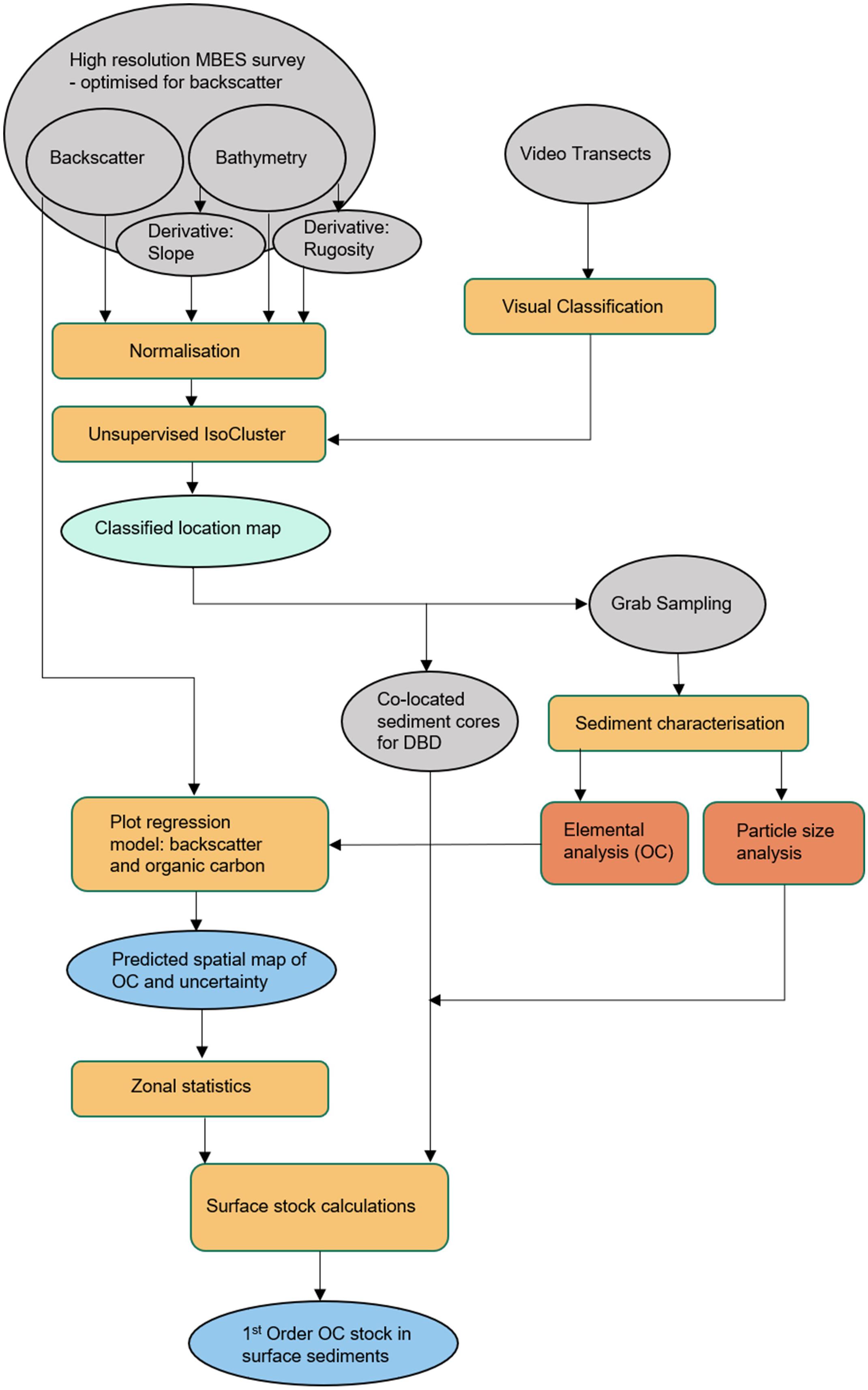
Figure 11. Schematic of our applied methodology which adapts existing benthic mapping tools to produce high spatial resolution maps for organic carbon within surface sediments. Key: Grey – sample collection; Yellow – processing step; Green – intermediary output; Orange – sediment characterisation; Blue – primary output.

MBES Classification

Our unsupervised classification used a combined input of backscatter, bathymetry, and bathymetry derivatives, slope and rugosity. Choosing the optimum number of clusters in an unsupervised approach can be a subjective process; we took the confidence results from a ML classification and the qualitative analysis of benthic tow video footage of the seabed to select 7 classes. Despite the results being based on a relatively small sample-set, we do see differences in sedimentary physical and geochemical properties between these classes and believe this to be a useful approach to informing a representative sampling campaign. To assess the influence of backscatter, bathymetry, and derivatives rugosity and slope for predicting OC, we ran ordinary least-squares regression models on each component individually in addition to combining all four as a multivariate regression. The only correlation we found was between backscatter and OC. Although bathymetry has been identified as an important factor in accurately discriminating classification exercises (Che Hasan et al., 2014; Calvert et al., 2015) and the other variables (slope, rugosity) have been used successfully in other studies (Lucieer et al., 2013; Diesing et al., 2016), they do not appear significant for predicting OC within our study area.

Benthic Video Application

Video as a ground-truthing tool has the advantage of increased coverage to understand sediment variability and in validating the acoustic signal. This type of ground-truthing is already used regularly for benthic habitat mapping and can be used to classify habitats based on observations of substrate and species to a European Nature Information System (EUNIS)-level classification (Lucieer et al., 2013; Calvert et al., 2015). It presents an opportunity for interdisciplinary studies relating substrate, habitat, and sedimentary OC data to maximise efficiency of resources for marine sampling. Ideally the benthic tows would be coincident with grab sampling to better understand how representative the grab sampler had been. Analysis of images improves confidence in the representativeness of the co-located, recovered grab material. Our visual assessment potentially over-estimated the number of discrete sediment types within Loch Creran; nonetheless it proved a useful exercise in planning a sampling campaign and we would recommend the use of images to bolster information from physical samples where available.

Mapping Sediment OC Using MBES

Recent examples of spatial sedimentary OC products have been generated over large areas of the shelf (over scales of hundreds of kilometres) using a combination of interpolated low-density sample data and spatial modelling which have large predictive uncertainties (Wilson et al., 2018). Our methodology uses a combination of tools to construct a high-resolution spatial map of OC and has the potential to leverage existing MBES surveys to improve regional shelf mapping through calibration of sediment properties. In the same way that acoustic data are now considered a useful proxy for seabed substrates, this novel application of backscatter presents an exciting opportunity toward improved and focussed OC mapping with appropriate ground-truthing and geochemical analyses (Lamarche and Lurton, 2018).

Surface Carbon Stocks

The definition of a ‘blue C’ stock is defined by Howard et al. (2014) as ‘the total amount of OC stored in a blue C ecosystem of a known size.’; a blue C ecosystem further classified as C stored specifically in either mangrove, saltmarsh or seagrass meadow habitats. This definition does not account for the contribution made by sediments not associated with vegetation in long-term OC storage. However, a national blue C inventory for Scotland does recognise this contribution as a ‘geological blue C stock’ (Burrows et al., 2017) and increased research into sedimentary OC is improving our understanding of its value (Luisetti et al., 2019). We have developed a method to calculate a surficial C stock for our survey area which could be used to support marine C accounting estimates. Surface sediments in marine environments generally receive highly labile forms of marine-sourced OM from the water column which are remineralised quickly with enhanced loss through natural processes such as bioturbation and re-suspension (Arndt et al., 2013; Bauer et al., 2013). Seasonal cycles will also impact the amount of OM available for deposition and the rates of remineralisation at the sediment surface (Cathalot et al., 2012). Nonetheless, despite surface OC stocks being vulnerable to change, this method could play a role in the identification of surface ‘hotspots’ toward understanding the most efficient sedimentary carbon sinks. Our stock estimates are based on well-constrained bulk-density values which are generally lacking for marine sediments. Our results show that while fine muddy sediments have the highest proportion of OC within their matrix, mixed sediments containing some coarser material contribute more significantly to OC stocks. This is a similar finding to other studies of particulate OC and sediment composition (Flemming and Delafontaine, 2000; Diesing et al., 2017). Understanding the content of OC within surface sediments of varying environmental settings is therefore an important aspect of further research, potentially allowing the increasing availability of spatial sediment composition data to be used for more accurate OC predictions and stock assessments (Mitchell et al., 2019).

Conclusion

We have developed a novel methodology using acoustic backscatter data to produce a continuous high-resolution (2 × 2 m) spatial map of sedimentary OC within a Scottish fjord. We find that OC correlates with backscatter as a function of sediment composition and that fine, muddy sediments are enriched in OC within our coastal study. It is possible using representative bulk density values to calculate surface stocks using our spatial predictions of OC allowing the possibility of incorporating estimates for C-stock accounting for marine sediments (Scottish Government, 2018). This methodology could be adopted into marine spatial planning using existing frameworks to aid setting mapping priorities at local, regional and national scales through increased collaborative partnerships to leverage existing opportunities and resources (e.g., Kendall et al., 2018).

Data Availability Statement

All datasets generated for this study are included in the article/Supplementary Material.

Author Contributions

WA led the conception of the study with subsequent design led by CH. RC collected and provided the processed MBES data and benthic tow imagery. CH undertook the research, laboratory and data analysis, and wrote the first draft of the manuscript as part of her Ph.D. at the University of St Andrews under the supervision of WA, UD, and DD. UD, DD, CS, and WA provided the technical assistance with sampling, laboratory equipment and software. All authors contributed to the manuscript revisions and approved the submitted version.

Funding

This work received joint funding from the University of St Andrews and the MASTS pooling initiative (The Marine Alliance for Science and Technology for Scotland) and their support is gratefully acknowledged. MASTS is funded by the Scottish Funding Council (grant reference HR09011) and contributing institutions. Additionally this work was funded via a grant to WA from the Natural Environment Research Council/Biotechnology and Biological Sciences Research Council (NERC/BBSRC) (grant number BB/M026620/1).

Conflict of Interest

The authors declare that the research was conducted in the absence of any commercial or financial relationships that could be construed as a potential conflict of interest.

Acknowledgments

We would like to thank the Scottish Blue Carbon Forum in their support of this research. We wish to thank the British Geological Survey for acquiring and processing the MBES dataset and the benthic tow surveys collected aboard the RV White Ribbon with credit to crew members, Sam Faithfull and William Lewis. The help of Scottish Natural Heritage for processing our application for sampling within Loch Creran and those involved in the sediment sample collection aboard RV Morwena, namely Elena Lo Giudice Cappelli and Kirsty Black is greatly appreciated. The operators at Creran Marine were particularly accommodating during our sampling efforts. We wish to acknowledge and thank this support of our work. Finally, with thanks to Carys McCulloch for her contribution toward the image classification work.

Supplementary Material

The Supplementary Material for this article can be found online at: https://www.frontiersin.org/articles/10.3389/fmars.2020.00588/full#supplementary-material

Footnotes

^ http://www.exifpro.com/index.html

References

Ahmed, K. I., and Demšar, U. (2013). Improving seabed classification from Multi-Beam Echo Sounder (MBES) backscatter data with visual data mining. J. Coast. Conserv. 17, 559–577. doi: 10.1007/s11852-013-0254-3