 Janaka Bamunawala1,2*Ali Dastgheib2Roshanka Ranasinghe1,2,3Ad van der Spek4,5
 Shreedhar Maskey2A. Brad Murray6Patrick L. Barnard7Trang Minh Duong1,2,3T. A. J. G. Sirisena1,2
- 1Department of Water Engineering & Management, University of Twente, Enschede, Netherlands
- 2IHE Delft Institute for Water Education, Delft, Netherlands
- 3Harbour, Coastal and Offshore Engineering, Deltares, Delft, Netherlands
- 4Applied Morphodynamics, Deltares, Delft, Netherlands
- 5Department of Physical Geography, Faculty of Geosciences, Utrecht University, Utrecht, Netherlands
- 6Division of Earth and Ocean Sciences, Nicholas School of the Environment, Center for Nonlinear and Complex Systems, Duke University, Durham, NC, United States
- 7United States Geological Survey, Pacific Coastal and Marine Science Center, Santa Cruz, CA, United States
Inlet-interrupted sandy coasts are dynamic and complex coastal systems with continuously evolving geomorphological behaviors under the influences of both climate change and human activities. These coastal systems are of great importance to society (e.g., providing habitats, navigation, and recreational activities) and are affected by both oceanic and terrestrial processes. Therefore, the evolution of these inlet-interrupted coasts is better assessed by considering the entirety of the Catchment-Estuary-Coastal (CEC) systems, under plausible future scenarios for climate change and increasing pressures due to population growth and human activities. Such a holistic assessment of the long-term evolution of CEC systems can be achieved via reduced-complexity modeling techniques, which are also ably quantifying the uncertainties associated with the projections due to their lower simulation times. Here, we develop a novel probabilistic modeling framework to quantify the input-driven uncertainties associated with the evolution of CEC systems over the 21st century. In this new approach, probabilistic assessment of the evolution of inlet-interrupted coasts is achieved by (1) probabilistically computing the exchange sediment volume between the inlet-estuary system and its adjacent coast, and (2) distributing the computed sediment volumes along the inlet-interrupted coast. The model is applied at three case study sites: Alsea estuary (United States), Dyfi estuary (United Kingdom), and Kalutara inlet (Sri Lanka). Model results indicate that there are significant uncertainties in projected volume exchange at all the CEC systems (min-max range of 2.0 million cubic meters in 2100 for RCP 8.5), and the uncertainties in these projected volumes illustrate the need for probabilistic modeling approaches to evaluate the long-term evolution of CEC systems. A comparison of 50th percentile probabilistic projections with deterministic estimates shows that the deterministic approach overestimates the sediment volume exchange in 2100 by 15–30% at Alsea and Kalutara estuary systems. Projections of coastline change obtained for the case study sites show that accounting for all key processes governing coastline change along inlet-interrupted coasts in computing coastline change results in projections that are between 20 and 134% greater than the projections that would be obtained if only the Bruun effect were taken into account, underlining the inaccuracies associated with using the Bruun rule at inlet-interrupted coasts.
Introduction
The coastal zone is the dynamic link that connects the land and oceans and has always attracted human settlement because of its multiple uses, rich bio-diversity and resources. Due to the many activities that are of great importance to society [e.g., navigation and access, defense and military, tourism, use of various marine/ecosystem resources and services, waste disposal, development of various coastal infrastructures, research, art, and recreational activities (McGranahan et al., 2007; Wong et al., 2014; Neumann et al., 2015)], the Low Elevation Coastal Zone (LECZ) is heavily urbanized and comprises approximately 10% of the world’s population (Vafeidis et al., 2011). Due to predicted population growth, economic development and urbanization, human pressures on coasts and coastal ecosystems will very likely increase significantly over the 21st century, with over 1 billion people expected to live in the coastal zone by 2050 (Hugo, 2011; Wong et al., 2014; Merkens et al., 2016). Apart from human-induced pressures, physical (environmental) forcing also places stresses on this environment, where projected climate-change driven variations in mean sea level, wave conditions, intensity and frequency of storm surges, and river flow will affect the coastal zone in many ways (FitzGerald et al., 2008; Syvitski and Kettner, 2008; Ranasinghe and Stive, 2009; Syvitski et al., 2009; Woodruff et al., 2013; Brown et al., 2014; Wong et al., 2014; Ranasinghe, 2016; Spencer et al., 2016). Rising sea level is likely to inundate many low-lying communities (Neumann et al., 2015; Ranasinghe, 2016). In conjunction with rising sea level, regional changes in wave and storm conditions and increased river flows will likely result in more frequent and intense episodic coastal flooding (Ranasinghe, 2016). Future changes in river flow will also directly control the amount of sediment received by coasts and subsequently transported onto beaches. Changes in fluvial sediment supply to the coast will affect flooding and erosion of low-lying coastal areas as beaches are the first line of defense for coastal hazards (Syvitski et al., 2009; Dunn et al., 2018, 2019; Besset et al., 2019). The potential socio-economic impacts of climate-driven flooding and beach losses are likely to be enormous. For example, forced migration due to sea-level rise driven coastline recession over this century is expected to cost about 1 trillion USD (Hinkel et al., 2013) while the potential economic losses in coastal cities due to flooding are expected cost more than 1 trillion USD by 2050 (Hallegatte et al., 2013) if the appropriate adaptation strategies are not implemented. Some other studies have shown that, under extreme emission and sea-level rise scenarios, average annual damage due to coastal flooding in Europe may also cost about 1.5 billion euros while affecting millions of people by the end of the 21st century if no new adaptation measures are taken in future (Bosello et al., 2012; Prahl et al., 2018; Vousdoukas et al., 2018, 2020a; Kirezci et al., 2020).
Coasts are highly varied and complex systems, and although the variety of coastal classifications is large, there is a societal need to focus on increasing our understanding of systems with pronounced anthropogenic influences and hazard risk. Here, we focus on sandy coasts, which comprise about one-third of the world’s coastlines (Luijendijk et al., 2018). Sandy coasts are considered to be one of the most complex coastal systems because the physical forcing acting on them and their geomorphic response are continually changing due to the influences of both natural and anthropogenic drivers (Ranasinghe, 2016; Toimil et al., 2017). The majority of these sandy coasts is interrupted by inlets (Aubrey and Weishar, 1988; Davis and Fitzgerald, 2003; Woodruff et al., 2013; FitzGerald et al., 2015; Duong et al., 2016; McSweeney et al., 2017). It should be noted that all the inlet-interrupted coasts are not necessarily connected with estuaries. Here, we focus on inlet-interrupted mainland coasts that are attached to estuaries receiving non-trivial river flows. These inlet-interrupted coasts are highly dynamic due to being governed by the interplay of oceanic and terrestrial processes (Stive, 2004; Ranasinghe et al., 2013; Anthony et al., 2015; Ranasinghe, 2016; Besset et al., 2019). Furthermore, as discussed above, climate change and anthropogenic activities in the coastal zone are likely to exert substantial changes to the complex and dynamic behavior of inlet-interrupted coasts. Such changes along inlet-interrupted coasts could lead even direr socio-economic impacts on this type of coasts compared to uninterrupted coasts, making a bad situation worse. Therefore, it is important to understand the physical responses of inlet-interrupted coasts under the plausible range of future variations in environmental forcing and anthropogenic activities.
Potential climate-change impacts on inlet-interrupted coasts can vary widely both on spatial and temporal scales. Climate-change impacts on sandy coasts are generally classified as short-term (hours to days), medium-term (years to decadal), and long-term (decades to century) with changes in sea level, wave conditions and storm surges, and river flow patterns being the primary climate-related impact drivers (Ranasinghe, 2016). Owing to the slow nature of rising sea level, coastal responses driven by sea-level rise will also be relatively slow. Under the Bruun effect, the coast will retreat as sediment shifts in the cross-shore direction across the nearshore seabed (Bruun, 1962) and potentially across subaerial portions of the coastal landscape [e.g., Wolinsky and Murray (2009), Dean and Houston (2016), Murray and Moore (2018)]. Additionally, inlet-interrupted coasts will undergo further coastal recession due to sea-level rise driven basin infilling as well (Stive et al., 1990, 1998; Stive, 2004; Ranasinghe et al., 2013). Along with these influences, future changes in temperature, precipitation and anthropogenic activities at catchment scale will alter the fluvial sediment supply received by the coasts (Syvitski and Milliman, 2007; Overeem and Syvitski, 2009; Syvitski et al., 2009; Ranasinghe et al., 2019), which in turn would affect sedimentation patterns, including beach behavior on inlet-interrupted coasts (Bamunawala et al., 2018a, 2020).
There are significant uncertainties in future climate change and anthropogenic driven impacts that could affect shoreline changes along sandy coasts (Ranasinghe, 2016, 2020; Le Cozannet et al., 2017). As a result, in addition to the uncertainties associated with the modeling techniques (i.e., model uncertainties), model-derived projections of future changes along inlet-interrupted coastlines will inherit the uncertainties related to the climate-related impact drivers and anthropogenic activities (i.e., input uncertainties) considered. Therefore, it is necessary to quantify the uncertainties associated with the shoreline change projections to better inform adaptation measures to manage the impacts of future climate change and anthropogenic activities, including potential socio-economic losses. Such measures will avoid unnecessary restrictions that are usually associated with conventional deterministic estimates of future coastline changes, thus enabling optimum utilization of the highly valuable land areas along coasts (Jongejan et al., 2016; Dastgheib et al., 2018). The added value of risk-informed coastal zone planning and management strategies (e.g., economically optimal setback lines) is amply illustrated by Jongejan et al. (2016) and Dastgheib et al. (2018), where the Probabilistic Coastal Recession (PCR) model (Ranasinghe et al., 2012) was applied to determine economically optimal coastal setback lines at the Narrabeen Beach, Sydney, Australia, and along the eastern coast of Sri Lanka, respectively.
Here, we develop a probabilistic modeling framework that can quantify the input uncertainties in the long-term evolution of CEC systems. Probabilistic estimates of coastline change along inlet-interrupted coasts under climate-change impacts and anthropogenic activities require multiple realizations using stochastic model inputs (i.e., Monte Carlo simulations). Hypothetically, if unlimited computational resources were available, such probabilistic modeling applications could be undertaken with coupled, highly detailed (i.e., hydrodynamics resolving) coastal and catchment models for the entire period considered so that the episodic (e.g., storms, surges, extreme river flows), medium-term (e.g., changes in river flow/mean wave conditions) and long-term impacts (e.g., sea-level rise, changes in fluvial sediment supply and longshore sediment transport capacity) due to climate change are deterministically accounted for in assessing the changes along inlet-interrupted coasts. However, the use of such highly detailed modeling techniques for ∼100-year simulations is impractical due to computational restrictions, or necessarily accurate, due to the potential cascade of model imperfections through temporal and spatial upscaling (Murray, 2007), as well as the accumulation of numerical errors within the computational domain during long-term simulations, which in turn may lead to morphological instabilities (Duong et al., 2016; Ranasinghe, 2016, 2020). Even if such a multi-scale highly detailed modeling technique were developed, the computational demand and the simulation time per each model realization would likely to make it impractical to be used in a probabilistic framework to estimate the coastline changes along inlet-interrupted coasts (Ranasinghe, 2016, 2020). These drawbacks can be overcome via the use of reduced-complexity models, which have proven to be very useful in obtaining insights into long-term coastal zone evolution at regional scales at low computational cost (Ranasinghe, 2016, 2020; van Maanen et al., 2016; Bamunawala et al., 2020). Due to their computational efficiency (compared to highly detailed models), reduced complexity models can be easily applied within a probabilistic framework to quantify the uncertainties in future changes along inlet-interrupted coastlines.
Here, a novel probabilistic modeling framework is presented to quantify the input uncertainties associated with projections derived from the reduced complexity model developed and demonstrated (albeit in deterministic mode) by Bamunawala et al. (2020). To enable a direct comparison of the two modeling approaches (i.e., deterministic vs. probabilistic), the probabilistic approach presented here is applied to the same coastal systems used by Bamunawala et al. (2020).
Materials and Methods
The reduced complexity model used here is described in detail by Bamunawala et al. (2020), and therefore, only a summary is presented below. In this model (G-SMIC), which is based on the SMIC model originally presented by Ranasinghe et al. (2013), the long-term evolution of inlet-interrupted coasts is represented by combining two major components: (1) coastline change due to the variation in total sediment volume exchanged (ΔVT) between the estuary and the adjacent inlet-interrupted coast, (2) sea-level rise-driven landward movement of the coastline (i.e., the Bruun effect).
Determining Changes in Total Sediment Volume Exchange Between an Estuary and the Adjacent Inlet-Interrupted Coast
Assuming that the coastal-estuary system is in dynamic equilibrium, the variation in total sediment volume exchanged (ΔVT) between the estuary system and its adjacent inlet-interrupted coast is calculated as a summation of three processes (Ranasinghe et al., 2013), given by the following equation.
where ΔVT is the cumulative change in the total sediment volume exchange between the estuary and its adjacent coast, ΔVBI is the sediment demand of the basin due to sea-level rise-driven change in basin volume (i.e., basin infilling volume), ΔVBV is the change in basin volume due to variation in river discharge, and ΔVFS is the change in fluvial sediment supply due to combined effects of climate change and anthropogenic activities, with all volumes in m3. A brief description of the three sediment volume components of equation [1] is given below [for detailed derivations, please see Ranasinghe et al. (2013) and Bamunawala et al. (2020)].
Basin Infilling Volume Due to Sea-Level Rise-Induced Increase in Accommodation Space
Rising sea level creates an additional volume within the basin. This additional volume (i.e., accommodation space) results in an extra sediment volume demand by the basin (ΔVBI), which can be computed as:
where Ab is the basin surface area (m2), “fac” (0 < fac < 1) accounts for the morphological response lag that exists between the hydrodynamic forcing (i.e., sea-level rise) and resulting morphological response of the basin [i.e., basin infilling volume (ΔVBI)]. In this study, the value of “fac” is set as 0.5 for all the simulations [adopted from Ranasinghe et al. (2013)].
Basin Volume Change Due to Variation in River Flow
The ebb-tidal flow volume of estuaries may change due to variations in future river flow. Such a change in the ebb-flow volume induces variations in estuarine and inlet flow velocities. In the process of striving to achieve its initial equilibrium flow velocity, an inlet-estuary system will therefore undergo changes in its channel cross-section and bed level. Such variations in the inlet-estuary system are associated with a specific volume of sediment (ΔVBV) exchanged between the inlet-estuary system and the adjacent inlet-interrupted coast, which can be calculated as:
where QR is the present river flow into the basin during ebb, ΔQR is the climate change-driven variation in river flow during ebb, VB is the present basin volume, and P is the mean equilibrium ebb-tidal prism, all volumes in m3.
Change in Fluvial Sediment Supply
Future changes in climate and anthropogenic activities at the catchment scale will result in changing the annual fluvial sediment supply received by an inlet-estuary system (Vörösmarty et al., 2003; Syvitski, 2005; Palmer et al., 2008; Ranasinghe et al., 2019). This change in fluvial sediment supply [ΔVFS (m3)] over the t (years) period considered can be calculated as:
where ΔQS is the change in annual fluvial sediment supply (m3).
Bamunawala et al. (2018a) and Bamunawala et al. (2020) have demonstrated that the empirical model presented by Syvitski and Milliman (2007) can be used to calculate the annual fluvial sediment throughput at the catchment scale.
where ω is a coefficient equal to 0.02 or 0.0006 for the annual fluvial sediment supply (QS) expressed in kg/s or MT/year at catchments, in which mean annual temperature is greater than 2°C, Q is the annual cumulative river discharge (km3), A is the river catchment area (km2), R is the catchment relief (km), and T is the catchment-wide mean annual temperature (°C). Note that equation [5] does not automatically account for any limitation in catchment-wide sediment volume generation. Therefore, in catchments with known limits to sediment generation, an appropriate threshold should be considered to limit the catchment-wide sediment production.
The catchment sediment production capacity is represented by the term “B” of the above equation, which is expressed as the following equation.
where L is the lithology factor that represents the catchment’s soil type and erodibility, ΔVT is the catchment-wide reservoir trapping efficiency factor, and Eh is catchment’s human-induced erosion factor.
The term I of the above equation [6] is the glacial erosion factor, which can be calculated according to the following equation.
where Ag is the ice cover percentage within the catchment area.
Syvitski and Milliman (2007) have suggested a range of factors for the human-induced erosion factor (0.2 ≤ Eh ≤ 2.0) by considering the population density of the country and its Gross National Production (per capita). However, this human-induced erosion factor (Eh) can be better approximated by the use of high-resolution Human FootPrint Index (HFPI) spatial data (Balthazar et al., 2013; Bamunawala et al., 2018a, 2020).
G-SMIC utilizes four main drivers to compute the change in total sediment volume exchange (ΔVT) between the estuary and the adjacent inlet-interrupted coast: annual mean temperature (T), annual cumulative river discharge (Q), change in regional relative sea-level (ΔRSL), and human-induced erosion factor (Eh). The climatic inputs (i.e., T and Q) are obtained from the Coupled Model Intercomparison Project Phase 5 (i.e., CMIP5) General Circulation Models (i.e., GCMs) (Taylor et al., 2011). There are unavoidable uncertainties associated with GCM projections. Similarly, the values obtained from different GCMs for the same Representative Concentration Pathway (RCP) also vary. Despite the inherent uncertainties among different GCM projections, many climate-change impact assessment studies use GCM outputs to drive future impact models. Projections of sea-level change also contain uncertainties. Human activities that may exert changes to the natural environment also vary along various dimensions (e.g., population growth, urbanization, and economic development). The probabilistic approach developed in this study quantifies the uncertainty in ΔVT arising from these input-uncertainties through stochastic treatment of the input variables.
In this study, the modeling period is defined as 2020–2100. Similar to the method adopted in Bamunawala et al. (2020), catchment-estuary-coastal (CEC) system conditions in 2019 were used as the reference condition in all the simulations. The climatic conditions over the last decade (i.e., 2010–2019) were used to determine the baseline values of T and Q (from CMIP5 GCMs) in all the model applications, to avoid the potentially biased representation of reference climatic conditions that would arise if only 2019 T and Q values were used.
Probabilistic Assessment of Change in Total Sediment Volume Exchange at an Estuary-Inlet System
The logical sequence of the probabilistic modeling approach adopted here is presented in Figure 1, followed by a description of the different computational steps involved.
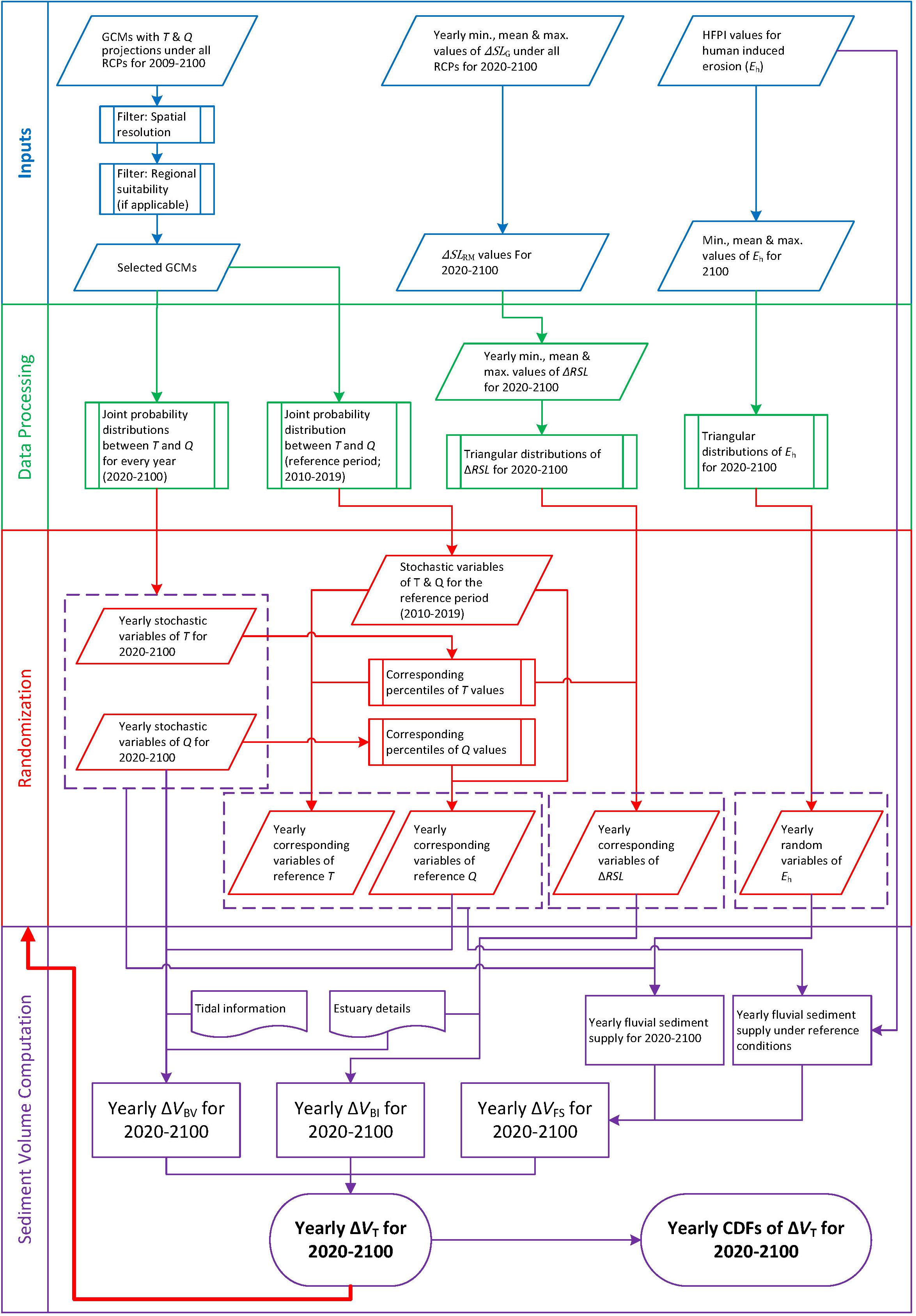
Figure 1. Flowchart of the modeling approach adopted to probabilistically determine the change in total sediment volume exchange between an estuary system and its adjacent inlet-interrupted coast.
Input Data
Temperature and runoff data for the 2009–2100 period (including the 2010–2019 reference period) were obtained from the General Circulation Models (GCMs) from the Coupled Model Intercomparison Project Phase 5 (CMIP5 data portal; Earth System Grid-Centre for Enabling Technologies (ESG-CET); available at http://pcmdi9.llnl.gov/). Projected values of temperature and surface runoff were obtained for all four RCPs of selected GCMs based on parameter output availability. Initially, GCMs with both temperature and surface runoff projections for four RCPs over the 2020–2100 period were considered as data sources. Out of these, GCMs with spatial resolution finer than 2.5° were selected to obtain the necessary climate inputs (T and Q). Further, where possible, the suitability of the above-selected data sources was assessed regionally, by considering published regional guidelines on model selection [e.g., CSIRO, and Bureau of Meteorology (2015) for Australia]. Based on these criteria, four GCMs (i.e., GFDL-CM3, GFDL-ESM2G, and GFDL-ESM2M from NOAA, United States, IPSL-CM5A-MR from IPSL) were selected to obtain the required T and Q values. These four GCMs were also the source of T and Q values used for deterministic G-SMIC projections presented in Bamunawala et al. (2020).
The regional relative sea-level change (ΔRSL) values at the respective case study locations were calculated according to the following equation (Nicholls et al., 2011):
where ΔRSL is the change in relative sea level, ΔSLG is the change in global mean sea level, ΔSLRM is the regional variation in sea level from the global mean due to meteo-oceanographic factors, ΔSLRG is the regional variation in sea level due to changes in the earth’s gravitational field, and ΔSLVLM is the change in sea level due to vertical land movement, all values are in m.
IPCC projections of ΔRSL at a given location by 2100 can be determined from Figure TS. 23 of Stocker et al. (2013a) and the corresponding ΔSLG values were obtained from Table SPM. 2 of Stocker et al. (2013b). The difference between these two sets of values provides the cumulative contribution of ΔSLRM, ΔSLRG, and ΔSLVLM for 2100. The temporal variation of the above three components was assumed to vary linearly from 2000 to 2100 (Mehvar et al., 2016) to enable the computation of these SLR components at yearly time steps as required by G-SMIC.
Yearly minimum, mean, and maximum values of global sea-level change (ΔSLG) were calculated according to the following equation (Nicholls et al., 2011).
where ΔSLG is the change in global sea level (m) since 2000, “t” is the number of years since 2000, a1 is the trend in sea level change (m/yr), and a2 is the change in the rate of sea-level change trend (m/yr2). The a1 and a2 coefficient values were obtained from published literature (Mehvar et al., 2016).
The human-induced erosion factor (Eh), which contributes to catchment scale sediment generation is here represented via the Human FootPrint Index (HFPI). HFPI values within the catchment were rescaled linearly to fit the optimum scale of Eh suggested in the literature (Syvitski and Milliman, 2007). These rescaled HFPI values were then averaged over the catchment to determine a representative factor for human-induced erosion (Eh). Given the contemporary rate of population growth and urbanization, it is safe to assume that Eh will have increased by 2100. Owing to numerous uncertainties associated in such projections [e.g., Veerbeek (2017)], the increment of Eh by 2100 was assumed to follow a triangular distribution with a mean, minimum and maximum of respectively 15, 10, and 20 percent of its present-day value.
Data Processing
The next step of the proposed modeling framework involves data preparation (green box in Figure 1). Here, annual cumulative distribution functions (CDFs) of the four model input parameters [viz., mean annual temperature (T), annual cumulative river discharge (Q), regional relative sea-level change (ΔRSL), and human-induced erosion factor (Eh)] were developed, so that the required stochastic model inputs could be generated.
Precipitation, evapotranspiration, runoff, and groundwater flow are the main components of the total water budget at catchment scales, with temperature, evapotranspiration, and precipitation being closely correlated parameters (Trenberth et al., 2007; Hegerl et al., 2015). Since T and Q values are inter-related, it is necessary to consider their dependencies when generating the stochastic model inputs. In order to capture the correlation between T and Q, joint probability distributions were generated for every year between 2020 and 2100 to determine the annual mean temperature and cumulative river discharge values at the catchment scale. Joint probability distributions for the 2020–2100 period were created by using ensembles of T and Q values obtained from the selected GCMs. A joint probability distribution of T and Q for the reference conditions was also generated by the use of annual mean temperature and cumulative river discharge values for the 2010–2019 period, using the output of the selected GCMs for this period.
The yearly values of ΔRSL (obtained as described above) were used to fit triangular distributions to represent ΔRSL for each year (2020–2100). For the human-induced erosion factor (Eh), the above-adopted minimum, mean, and maximum increments by 2100 were assumed to be reached via a linear increase from 2020, and triangular distributions were fitted to represent yearly Eh values for the 2020–2100 period.
Generating Stochastic Model Inputs
The third stage of the proposed probabilistic modeling framework is devoted to generating the stochastic model input for temperature, river discharge, regional relative sea-level change, and the human-induced erosion factor (i.e., randomization; red box in Figure 1). The fitted joint probability distributions for temperature and river discharge were here used to generate stochastic model inputs for T and Q for each year (100,000 randomly pairs of T and Q per year) for the future period (2020–2100) and the reference period (2010–2019). For all the future T and Q between 2020 and 2100, reference values with the same probability of occurrences were selected (i.e., reference T and Q with the same percentiles as the future values).
The two main causes of global sea-level rise are thermal expansion (i.e., steric effect) caused by warming of the oceans and increased melting of land-based ice, such as glaciers and ice sheets (Stocker et al., 2013b). Both of these factors are directly related to increasing temperature. Therefore, in all the model applications, a direct relationship was assumed between annual mean temperatures (T) and change in regional relative sea-level (ΔRSL) (Rahmstorf, 2007). In order to achieve this direct relationship, percentiles of each annual mean temperature (T) value obtained through the fitted joint probability models (as described above) were calculated. The ΔRSL values with the same percentiles as T were selected from the fitted triangular distributions that represent the regional relative sea-level change (ΔRSL) for each year between 2020 and 2100 (100,000 values per year).
Fitted triangular distributions that represent the human-induced erosion factor (Eh) were used to generate stochastic variables of Eh for 2020–2100 (100,000 random values per each year).
Computing Sediment Exchange Volumes
All the above computed stochastic model inputs were then used in the final phase of the probabilistic modeling framework to determine the change in total sediment volume exchange (ΔVT) between a given estuary system and the adjacent inlet-interrupted coast (i.e., sediment volume computation; purple box in Figure 1). The above-computed Q values were used together with estuarine and tidal information to calculate the variations in sediment volume due to changes in basin volume (ΔVBV) during 2020–2100. Generated ΔRSL values were used together with estuarine information to determine the sediment volume demands due to basin infilling (ΔVBI) for 2020–2100. Changes in fluvial sediment supply (ΔVFS) were computed using the stochastically generated future and reference T and Q values, human-induced erosion factor values, and other required river catchment information. These three sediment volume components were then used to compute the total change in sediment volume exchange (ΔVT) (100,000 values per year), and empirical cumulative distributions of ΔVT were developed for each year over the 2020–2100 projection period.
Simplified One-Line Coastline Change Model
The simplified one-line coastline change model used here is also described in detail by Bamunawala et al. (2020), and hence only a summary of that modeling approach is presented below. This simplified approach assumes uniform coastline orientation and lack of any coastal structures along up- and down-drift coasts. It also adopts time-invariant longshore sediment transport rate and depth of closure value for all future coastline change projections. The maximum extent of inlet-affected coastline length is considered to be ∼25 km from an inlet. Otherwise, this distance from an inlet is constrained by the presence of rock outcrops, headlands, noticeable change in mean shoreline orientation or inlets. If there are no gradients in annual longshore sediment transport rates along up- and down-drift coasts, the coastal cell considered is assumed to be in equilibrium at annual time scales.
A selected percentile value of the above computed ΔVT can be used to determine the subsequent changes along the adjacent inlet-interrupted coast. Here, the 50th percentile values of ΔVT were used to determine the changes along the inlet-interrupted coasts. Since the ΔVT is computed annually, it is first divided into a number of equal fragments (nv). This volume fragment (Vfr) is then distributed along the adjacent coastline. Volume fragment (Vfr) is calculated using the following equation.
All or a part of this sediment volume fragment will be transported along the coast. This is closely related to the equivalent longshore sediment transport capacity at the vicinity (). Based on the assumption of a balanced sediment budget within the coastal cell, sediment volume that gets transported to the farthermost section of the down-drift coast will contribute to progradate that coastline. For eroding coastlines, computation is started from the section nearest to the inlet. If Vfr is larger than ΔQLST, the surplus sediment volume (ΔV = Vfr−ΔQLST) will result in prograding the shoreline (Δy) within the longshore distance considered (Δx) (Please refer to Supplementary Figure 1 for a schematic illustration of a hypothetical equilibrium cross-shore profile).
The magnitude of seaward translation (Δy) of the longshore distance (Δx) can be computed using the following equation when the shoreline is assumed to move cross-shore parallel to itself while maintaining the initial equilibrium profile.
where D is the depth of closure.
The above procedure is repeated within subsequent longshore distances (Δx) until a sediment volume fragment (Vfr) is distributed. Then the procedure is repeated nv times, so that the ΔVT is fully distributed within the coastal cell. These computations are closely related with an expression for longshore sediment transport rate (QLST), which can be expressed as the following equation.
where Q0 is the amplitude of the longshore sediment transport rate (m3/yr), and αb is the breaking wave angle, measured between the wave crest lines and coastline. This angle can be calculated using the following equation.
where α0 is the angle of breaking wave crests, measured relative to the coastline.
The coastline position (Δy) would be updated locally with the longshore distribution of every volume fragment (Vfr). Hence, the breaking wave angle (αb) and longshore sediment transport rate (QLST) are also update accordingly after the distribution of Vfr. Once the ΔVT is fully distributed, the final coastline position can be obtained by superimposing the coastline recession due to the Bruun effect (Bruun, 1962).
Case Study Sites and Stochastic Model Inputs
The above-presented modeling technique was applied to the case study locations considered in Bamunawala et al. (2020) (i.e., Alsea estuary, Oregon, United States, Dyfi estuary, Wales, United Kingdom, and Kalutara inlet, Sri Lanka; Supplementary Figure 2). Table 1 summarizes the key properties of the selected three systems [for more details, please see Bamunawala et al. (2020)].
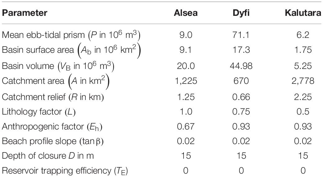
Table 1. Properties of the selected case study CEC systems [after Bamunawala et al. (2020)].
Figures 2–4 show the GCM derived projected variations of annual mean temperature (T) and the annual cumulative river discharge (Q) of the Alsea, Dyfi, and Kalu River catchments, respectively over the three decadal periods considered (2021–2030, 2056–2065, and 2091–2100). Figure 5 shows the projected variations in the mean, minimum, and maximum regional relative sea-level changes (ΔVT) in the vicinity of the Alsea, Dyfi, and Kalutara inlets over the 21st century.
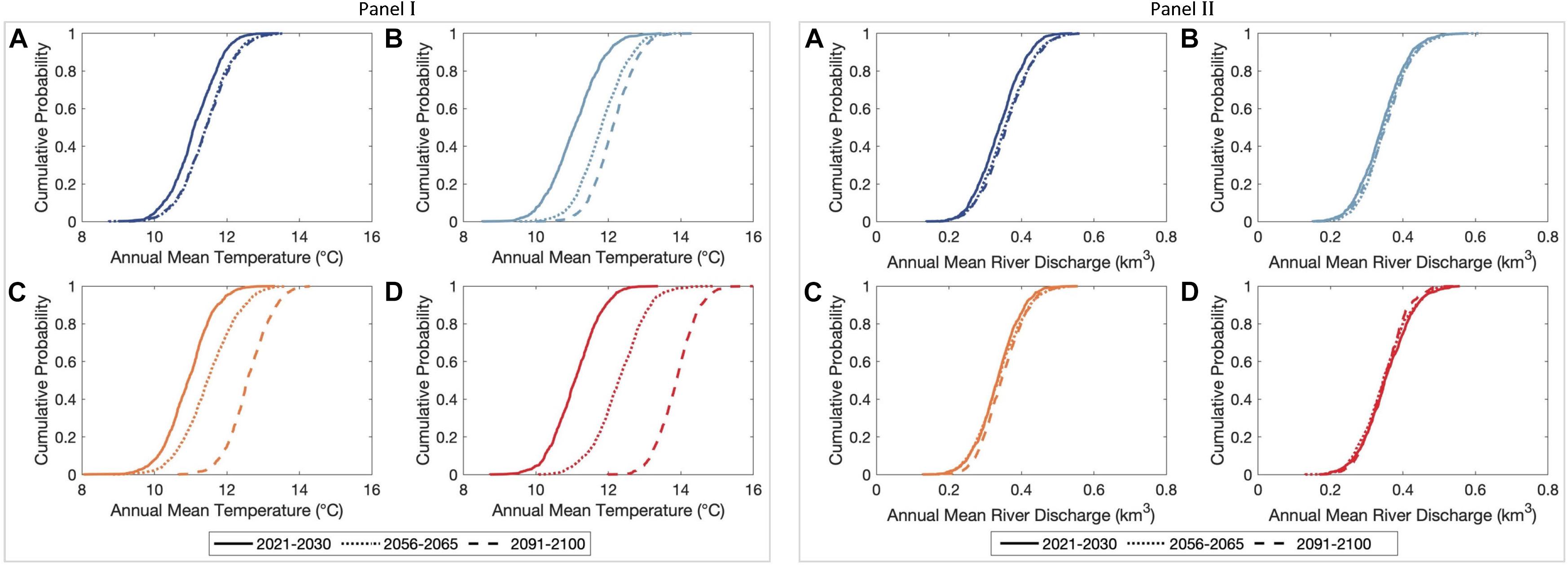
Figure 2. Empirical cumulative distributions of averaged annual mean temperature (Panel I) and the annual cumulative river discharge (Panel II) in the Alsea River catchment, Oregon, the United States over the three decadal periods considered. Subplots (A), (B), (C), and (D) are for the RCPs 2.6, 4.5, 6.0, and 8.5, respectively.
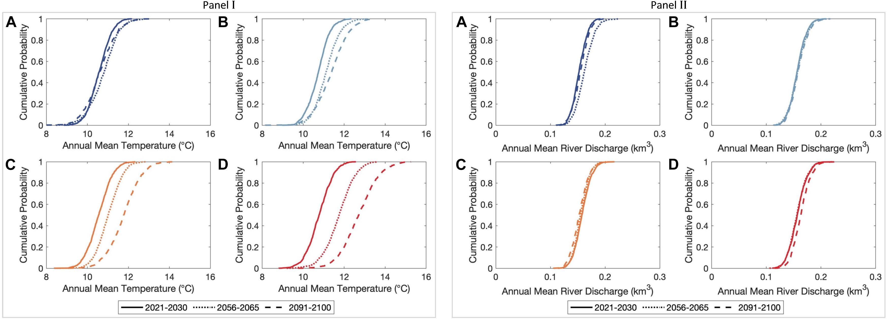
Figure 3. Empirical cumulative distributions of averaged annual mean temperature (Panel I) and the annual cumulative river discharge (Panel II) in the Dyfi River catchment, Wales, the United Kingdom over the three decadal periods considered. Subplots (A), (B), (C), and (D) are for the RCPs 2.6, 4.5, 6.0, and 8.5, respectively.
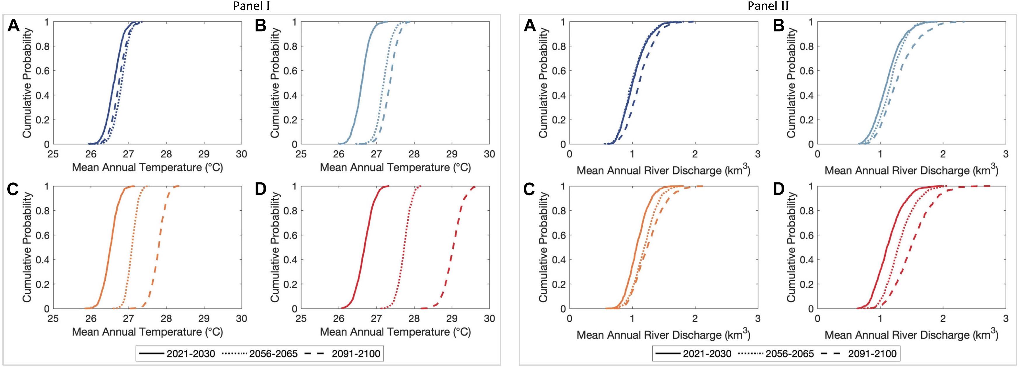
Figure 4. Empirical cumulative distributions of averaged annual mean temperature (Panel I) and the annual cumulative river discharge (Panel II) in the Kalu River catchment, Sri Lanka over the three decadal periods considered. Subplots (A), (B), (C), and (D) are for the RCPs 2.6, 4.5, 6.0, and 8.5, respectively.
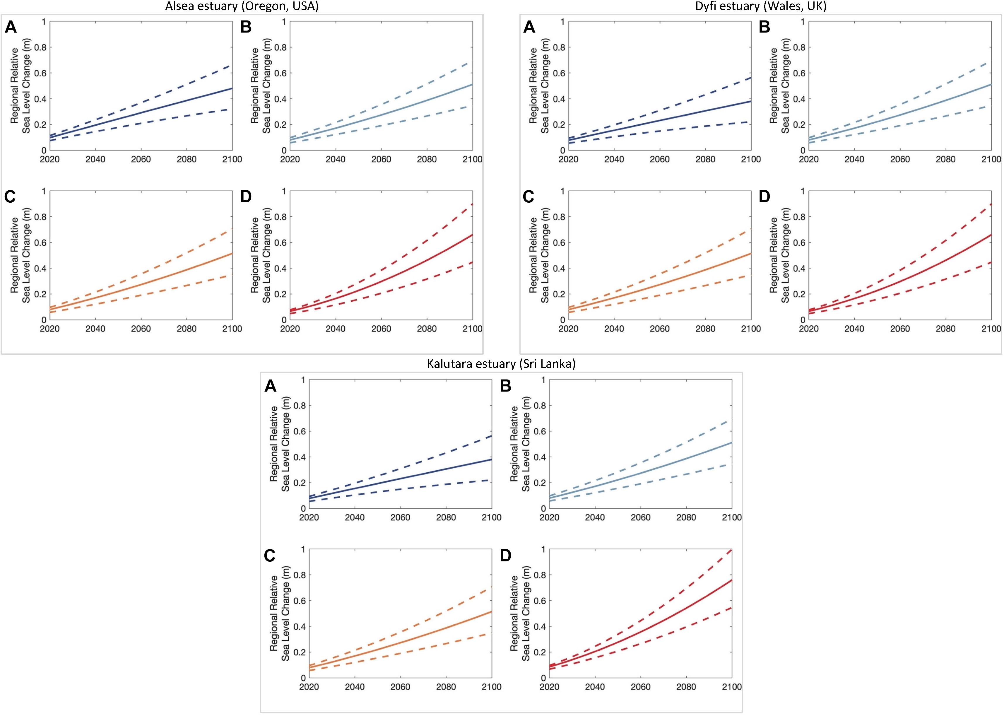
Figure 5. Projected changes in regional relative sea level in the vicinities of the three case study CEC systems. The solid line indicates the mean change, while the two dashed lines indicate the computed maximum and minimum values of ΔRSL. Subplots (A), (B), (C), and (D) are for the RCPs 2.6, 4.5, 6.0, and 8.5, respectively.
Similar to the globally averaged temperature variation published by Stocker et al. (2013b), the 50th percentile T values in Alsea river catchment show hardly any change during mid- and end-century periods for RCP 2.6 [Figure 2, Panel I, subplot (a)]. The projected maximum and minimum increments of the 50th percentile T values by 2100 are 3.0°C and 0.5°C for RCP 8.5 and 2.6, respectively. The projected variations in Q values of the Alsea River catchment indicate only minor variations over the 21st century for all RCPs (Figure 2, Panel II). Except for RCP 8.5, projected Q values are slightly increased by 2100 [relative to the early-century (2021–2030) period], where the maximum and minimum increments in the 50th percentile magnitudes are 0.2 km3/yr and <0.1 km3/yr for RCP 2.6 and 4.5, respectively. The projected 50th percentile Q value by 2100 is marginally decreased (<0.1 km3/yr) for RCP 8.5.
Unlike the globally averaged temperature variation published by Stocker et al. (2013b), the 50th percentile T values in the Dyfi River catchment show differences during mid- and end-century periods for RCP 2.6, in which the projections for the latter period (i.e., 2091–2100) are approximately 0.5°C warmer than the former duration [Figure 3, Panel I, subplot (a)]. The projected maximum and minimum increments of the 50th percentile T values by 2100 are 2.5°C and 0.5°C for RCP 8.5 and 2.6, respectively. The projected variations in Q values of the Dyfi River catchment indicate minor variations over the 21st century for all RCPs (Figure 3, Panel II). Except for RCP 6.0, the projected Q values are slightly increased by 2100 (relative to the early-century period). However, all these projected variations (i.e., both reductions and increments) are quite trivial, and thus only result in minor variations of Q (<0.05 km3/yr) in the Dyfi River catchment over the 21st century.
The 50th percentile T values in the Kalu River catchment also show differences during mid- and end-century periods for RCP 2.6, in which the latter period (i.e., 2091–2100) projection is approximately 0.25°C warmer than the former [Figure 4, Panel I, subplot (a)]. The projected maximum and minimum increments of the 50th percentile T values by 2100 are 2.5°C and <0.5°C for RCP 8.5 and 2.6, respectively. The projected variations in Q values in the Kalu River catchment indicate increased river discharge over the 21st century for all RCPs (Figure 4, Panel II). Except for RCP 2.6, the projected Q values are increased by 2050 as well (relative to early-century period). The projected maximum and minimum increments in the 50th percentile Q values by 2100 are 0.75 km3/yr and 0.25 km3/yr for RCP 8.5 and 2.6, respectively. The projections for RCP 8.5 indicated a small likelihood (∼1% probability of exceedance) of extreme discharges (about 3.0 km3/yr) over the latter part of the 21st century [Figure 4, Panel II, subplot (d)], which is about twice the magnitude of the 50th percentile Q values over the same period.
Figure 5 indicates that the projected mean change of ΔRSL by 2100 is largest in the vicinity of the Kalutara inlet system (Sri Lanka), whereas the minimum change by 2100 is projected for the Alsea estuary (Oregon, United States). However, the largest range (min-max) of projected ΔVBV by 2100 is projected in the vicinity of the Dyfi estuary (Wales, United Kingdom).
It should be noted that river sand mining activities are carried out along the Kalu River (Bamunawala et al., 2018b). The annual volume of this sand extraction is about 423,060 m3/yr, which is assumed to be linearly increased by 20% over the 2020–2100 simulation period.
Results
The results obtained by applying the above-described modeling approach to the three case study sites are presented in two steps: (1) probabilistic estimates of projected variations in the total sediment volume exchange (ΔVT) between the inlet-estuary systems and their adjacent coasts and (2) projected evolution of the inlet-interrupted coasts at the study sites.
Projected Variations of Total Sediment Volume Exchange (ΔVT) (2020–2100)
Alsea Estuary System
Figure 6 shows that, at Alsea estuary, both RCP 2.6 and 8.5 result in similar ranges of uncertainty and 50th percentile values of ΔVT during 2020–2050 [−0.5 Million Cubic Meters (MCM) by 2050]. From that point onward, the projected uncertainty ranges and the 50th percentile values of ΔVT under RCP 8.5 tend to deviate from those under RCP 2.6 and result in a much greater 50th percentile value by 2100 (−1.7 MCM). The projected uncertainties of ΔVT in 2100 are quite similar for all but RCP 8.5. The results also highlight that the deterministic projections of ΔVT for RCP 8.5 presented in Bamunawala et al. (2020) are consistently greater than the 50th percentile values of the probabilistic projections, by as much as 0.5 MCM (∼30%) by 2100.
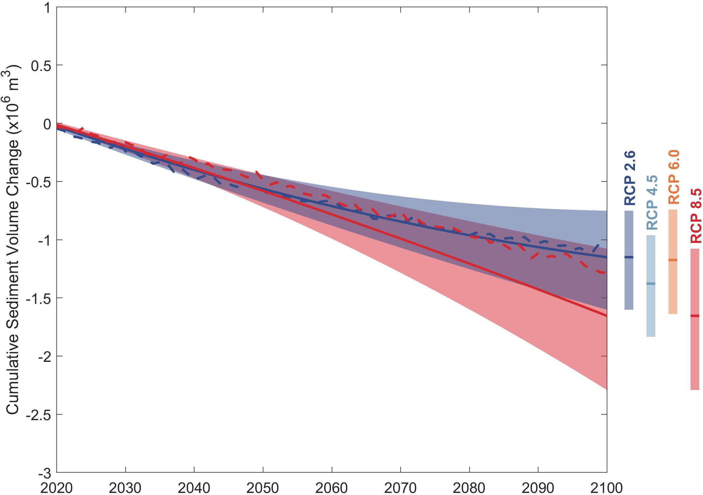
Figure 6. Projected variation of change in total sediment volume exchange (ΔVT) between the Alsea estuary and the adjacent coast over the 21st century. The projected ranges between 10th and 90th percentile are shown as shaded bands with the variation of the 50th percentile values indicated by the solid lines for RCP 2.6 (blue) and RCP 8.5 (red). The negative volumes indicate that the estuary traps more sediment at the expense of the open coast. Deterministic projections of ΔVT presented in Bamunawala et al. (2020) for RCP 2.6 (blue) and RCP 8.5 (red) are indicated by the dashed lines. Vertical bars indicate the projected ranges between the 10th and 90th percentiles in 2100 for all RCPs with the 50th percentile values indicated as horizontal lines.
The empirical CDF plots in Figure 7-Panel I indicate the total uncertainties associated with the projected ΔVT at the Alsea estuary system (in contrast to the selected range between 10th and 90th percentiles presented in Figure 6). During the first decadal period, there is very little uncertainty in the ΔVT projections under all four RCPs, as evidenced by almost vertical CDFs. These uncertainties increase slightly over the mid-century period for all RCPs (<0.25 MCM), increasing to considerable uncertainties by the end-century period, in which the least (0.75 MCM) and the most (1.0 MCM) variations by 2100 are projected for RCP 4.5 and 8.5, respectively. The results presented in Figure 7-Panel II indicate that the future evolution of ΔVT at Alsea estuary system will be governed by the basin infilling volume (ΔVBI). The results also indicate that the projected variations of ΔVBV have negligible impacts on ΔVT for all RCPs, because of the trivial changes in the projected annual cumulative river discharge values of this river catchment (Figure 2-Panel II).
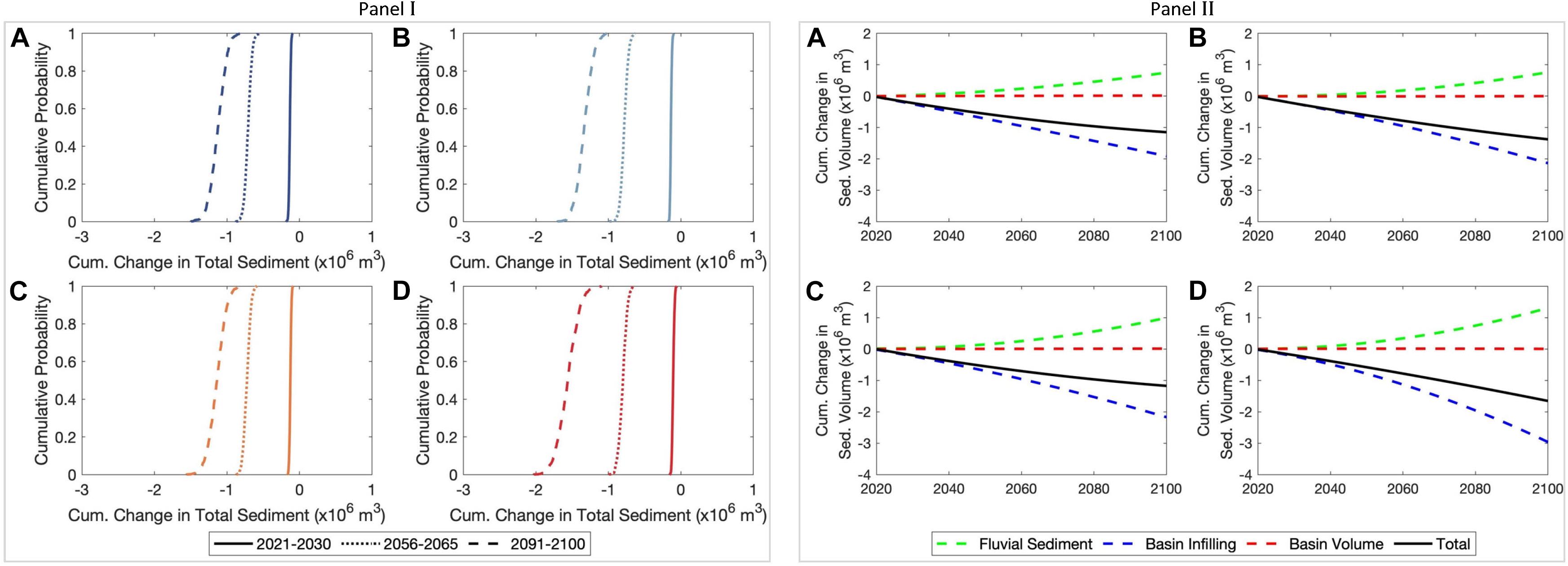
Figure 7. Empirical cumulative distributions of the projected change in total sediment volume exchange (ΔVT) between the Alsea estuary and the adjacent coast over the three decadal periods considered (Panel I). The empirical cumulative distributions were developed by averaging the projected ΔVT values over the three decadal periods considered. (Panel II) shows the computed variations of the projected 50th percentile values of change in total sediment volume exchange (ΔVT) and contributions from different processes to ΔVT at the Alsea estuary over the 21st century. Negative volumes indicate that the estuary traps more sediment at the expense of the open coast (i.e., sediment importing estuary). Subplots (A), (B), (C), and (D) are for the RCPs 2.6, 4.5, 6.0, and 8.5, respectively.
The sediment demand due to basin infilling (ΔVBI) is projected to increase rapidly during the late 21st century under RCP 8.5 [due to projected acceleration in ΔRSL under this scenario as shown in Figure 5-Alsea estuary (Oregon, United States)], thus resulting in the largest 50th percentile cumulative estuary sediment volume demand by 2100 (3.0 MCM). Projected changes in mean annual temperature (Figure 2-Panel I), and the human-induced erosion factor (Eh) contribute positively to the sediment balance by leading to increases in fluvial sediment supply (ΔVFS) toward the latter part of 2100 (i.e., after 2080) for all RCPs. The increase in fluvial sediment supply offsets the sea-level-rise-driven basin infilling volume demand. Therefore, the largest projected 50th percentile value of ΔVT in the Alsea estuary system by 2100 is −1.5 MCM under RCP 8.5.
Dyfi Estuary System
Figure 8 shows that, both RCP 2.6 and 8.5 result in similar ranges of uncertainties of ΔVT at the Dyfi estuary system during the 2020–2050 period. However, the magnitude of the 50th percentile value of ΔVT for RCP 8.5 (−1.5 MCM) is 50% larger than that for RCP 2.6 (−1.0 MCM) by 2050. From that point onward, projected uncertainty ranges and the 50th percentile values of ΔVT under RCP 8.5 tend to deviate from those under RCP 2.6 and result in 100% larger median value by 2100 (−5.0 MCM under RCP 8.5 compared to −2.5 MCM under RCP 2.6). The deterministic model results presented in Bamunawala et al. (2020) are similar to the 50th percentile values of ΔVT of the probabilistic projections.
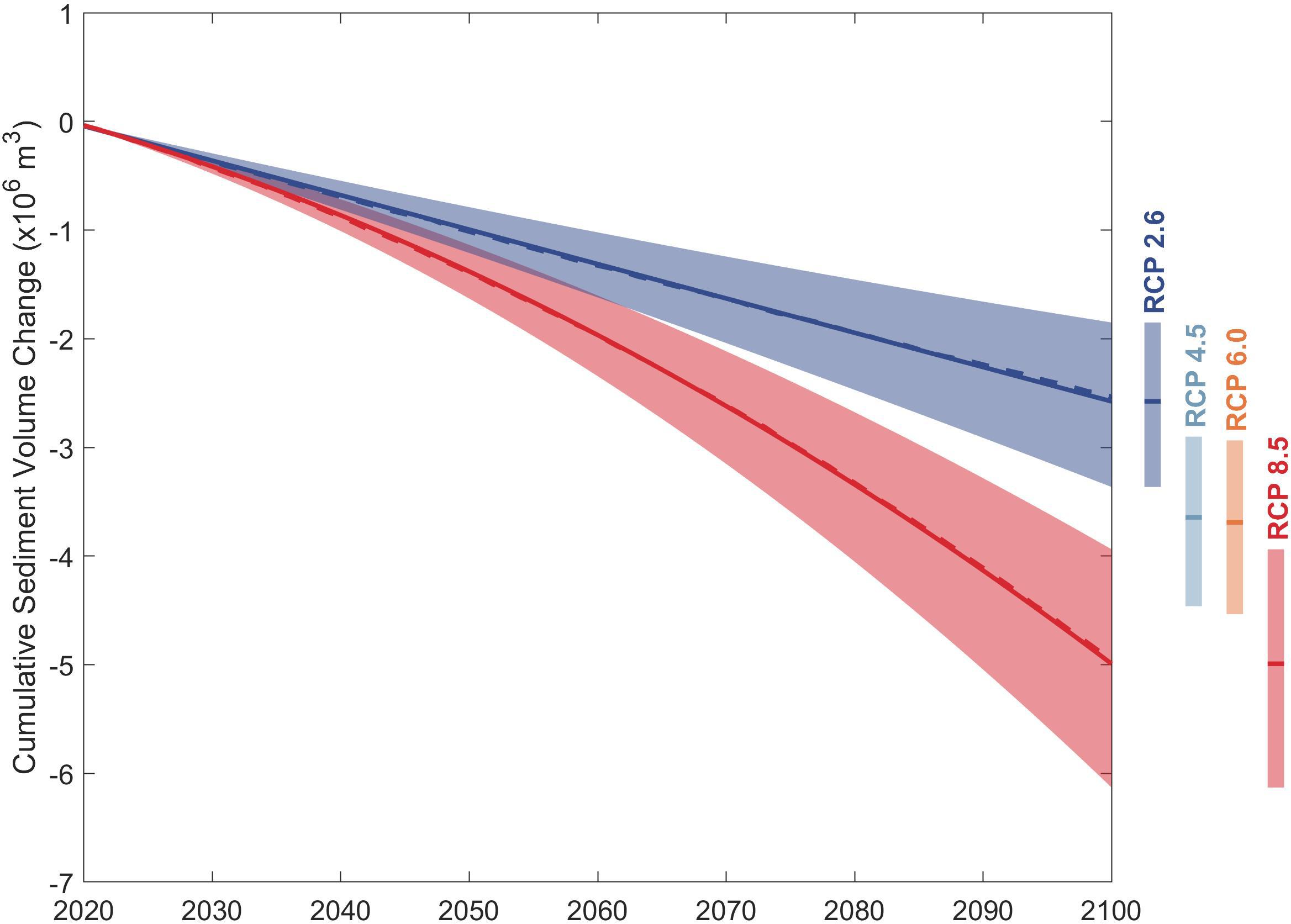
Figure 8. Projected variation of change in total sediment volume exchange (ΔVT) between the Dyfi estuary and the adjacent coast over the 21st century. The projected ranges between 10th and 90th percentile are shown as shaded bands with the variation of the 50th percentile values indicated by the solid lines for RCP 2.6 (blue) and RCP 8.5 (red). The negative volumes indicate that the estuary traps more sediment at the expense of the open coast. Deterministic projections of ΔVT presented in Bamunawala et al. (2020) for RCP 2.6 (blue) and RCP 8.5 (red) are indicated by the dashed lines. Vertical bars indicate the projected ranges between the 10th and 90th percentiles in 2100 for all RCPs with the 50th percentile values indicated as horizontal lines.
The empirical CDFs presented in Figure 9-Panel I indicate that the projections of ΔVT at the Dyfi estuary system show very little uncertainty under all four RCPs during the first decadal period (i.e., 2021–2030). These uncertainties increase slightly over the mid-century period (i.e., 2056–2065) for all RCPs (0.5 MCM), increasing to considerable uncertainties by the end-century period (i.e., 2091–2100), in which the largest (1.5 MCM) variations by 2100 are projected for RCP 8.5. The results presented in Figure 9-Panel II indicate that ΔVT at Dyfi estuary system is governed by basin infilling volume (ΔVBI) for all RCPs, and ΔVBV and ΔVFS have trivial impacts on projected ΔVT regardless of the RCP.
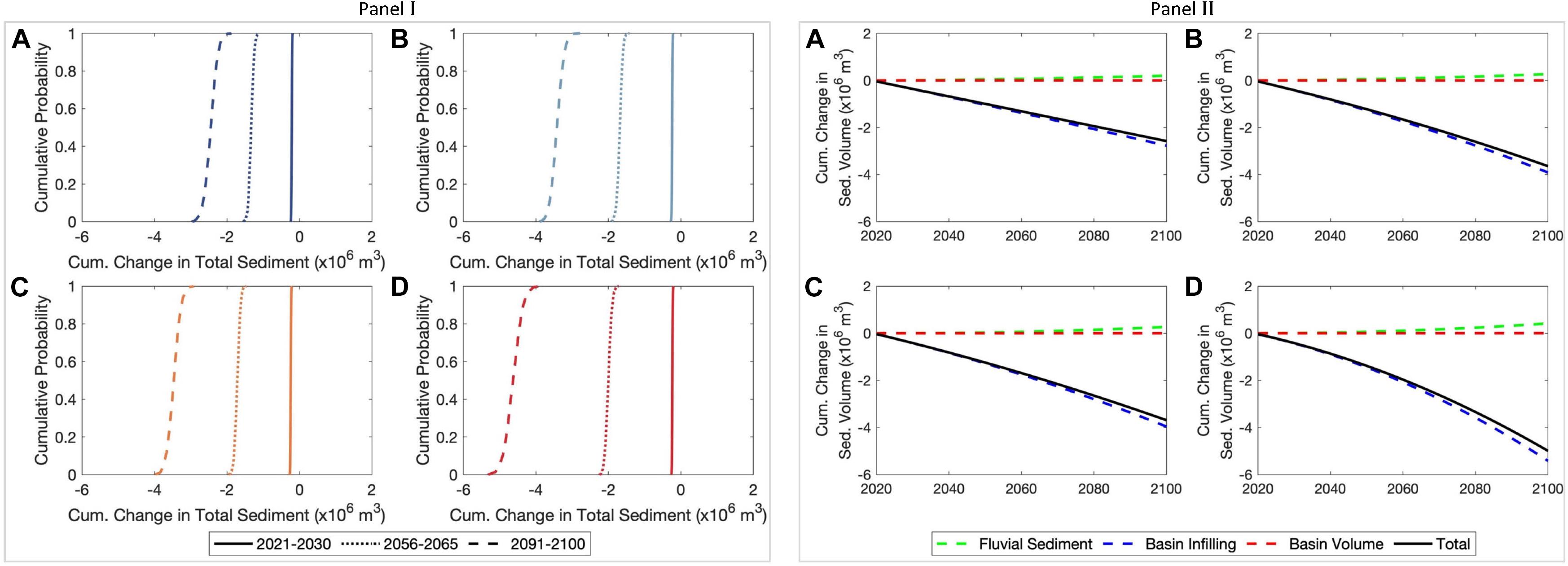
Figure 9. Empirical cumulative distributions of the projected change in total sediment volume exchange (ΔVT) between the Dyfi estuary and the adjacent coast over the three decadal periods considered (Panel I). The empirical cumulative distributions were developed by averaging the projected ΔVT values over the three decadal periods considered. (Panel II) shows the computed variations of the projected 50th percentile values of change in total sediment volume exchange (ΔVT) and contributions from different processes to ΔVT at the Dyfi estuary over the 21st century. Negative volumes indicate that the estuary traps more sediment at the expense of the open coast (i.e., sediment importing estuary). Subplots (A), (B), (C), and (D) are for the RCPs 2.6, 4.5, 6.0, and 8.5, respectively.
The relative contribution from ΔVBV is negligible because the projected changes in the annual cumulative river discharge values of the river catchment are trivial (Figure 3-Panel II). Despite the projected increments in mean annual temperature (Figure 3-Panel I) and the human-induced erosion (Eh), the projected increases in fluvial sediment throughput of the small Dyfi River catchment is not sufficient to noticeably offset the estuarine sediment demand due to the basin infilling process. The sediment demand due to basin infilling (ΔVBI) is projected to increase rapidly under RCP 8.5, especially during the late 21st century [due to the projected acceleration in ΔRSL under RCP 8.5; Figure 5-Dyfi estuary (Wales, United Kingdom)], thus resulting in the largest 50th percentile cumulative sediment volume demand by the estuary (5.5 MCM by 2100). The projected maximum and minimum 50th percentile values of ΔVT at Dyfi estuary system by 2100 are −2.5 MCM and −5.0 MCM for RCP 2.6 and 8.5, respectively.
Kalutara Inlet System
Figure 10 indicates that the 50th percentile value and the uncertainty in projected ΔVT at the Kalutara estuary system will increase gradually over the 21st century. Interestingly, however, the 50th percentile ΔVT under RCP 8.5 decreases until the mid-century and then increases toward the end-century period. The largest and the smallest magnitudes of the projected 50th percentile value of ΔVT by 2100 are 7.5 MCM and 3.5 MCM for RCP 2.6 and 8.5, respectively. The deterministic projections of ΔVT for RCP 2.6 presented in Bamunawala et al. (2020) is about 15% larger than the 50th percentile values of the probabilistic projections by the end of the 21st century.
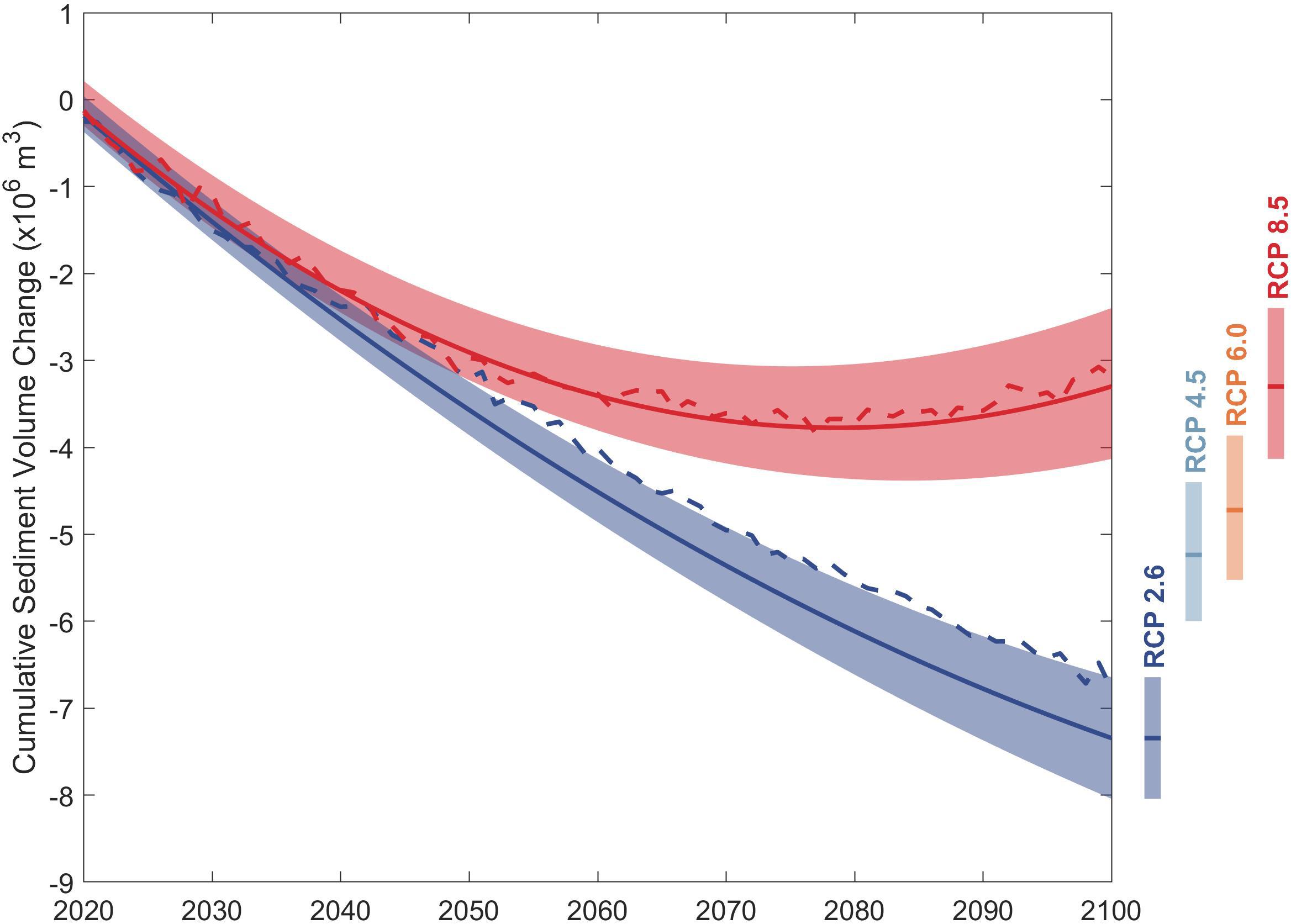
Figure 10. Projected variation of change in total sediment volume exchange (ΔVT) between the Kalutara estuary and the adjacent coast over the 21st century. The projected ranges between 10th and 90th percentile are shown as shaded bands with the variation of the 50th percentile values indicated by the solid lines for RCP 2.6 (blue) and RCP 8.5 (red). The negative volumes indicate that the estuary traps more sediment at the expense of the open coast. Deterministic projections of ΔVT presented in Bamunawala et al. (2020) for RCP 2.6 (blue) and RCP 8.5 (red) are indicated by the dashed lines. Vertical bars indicate the projected ranges between the 10th and 90th percentiles in 2100 for all RCPs with the 50th percentile values indicated as horizontal lines.
During the first decadal period (i.e., 2021–2030), ΔVT at the Kalutara inlet-estuary system shows very little uncertainty under all four RCPs (Figure 11-Panel I). These uncertainties increase slightly over the mid-century period (i.e., 2056–2065) for all RCPs (1.0 MCM), increasing to considerable uncertainties by the end-century period (i.e., 2091–2100), with the largest (5.0 MCM) uncertainty under RCP 8.5. Figure 11-Panel II indicate that ΔVT at the Kalutara estuary system is governed by the fluvial sediment supply (ΔVFS) under all RCPs and the projected variations of ΔVBV and ΔVBI have trivial impact on ΔVT regardless of the RCP.
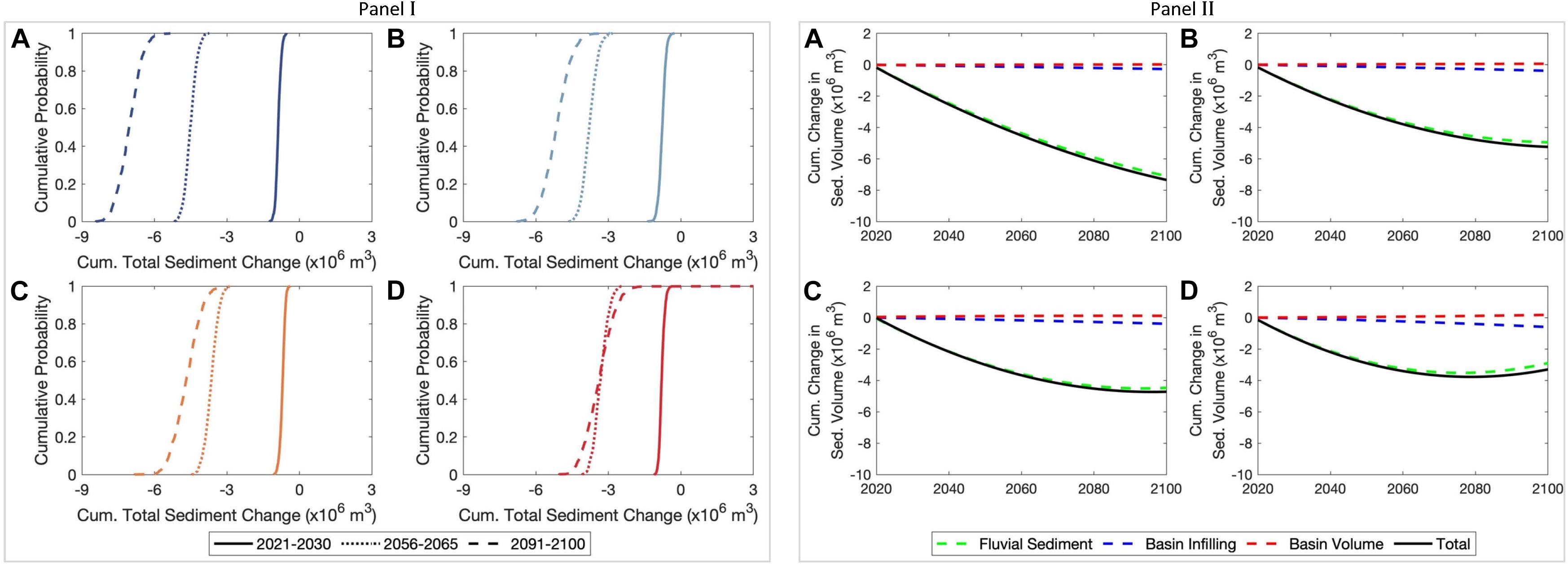
Figure 11. Empirical cumulative distributions of the projected change in total sediment volume exchange (ΔVT) between the Kalutara estuary and the adjacent coast over the three decadal periods considered (Panel I). The empirical cumulative distributions were developed by averaging the projected ΔVT values over the three decadal periods considered. (Panel II) shows the computed variations of the projected 50th percentile values of change in total sediment volume exchange (ΔVT) and contributions from different processes to ΔVT at the Kalutara estuary over the 21st century. Negative volumes indicate that the estuary traps more sediment at the expense of the open coast (i.e., sediment importing estuary). Subplots (A), (B), (C), and (D) are for the RCPs 2.6, 4.5, 6.0, and 8.5, respectively.
The largest projected 50th percentile cumulative sediment volume demand by the Kalutara estuary in 2100 is 7.0 MCM for RCP 2.6. This is due to the reduction in fluvial sediment supply as a result of river sand mining in this system. In this case, the projected increases in fluvial sediment supply due to increased T (Figure 4, Panel I), and Q (Figure 4, Panel II) under RCP 2.6 are unable to compensate for river sand mining at any time in the 21st century. Despite the same reduction in fluvial sediment due to river sand mining, fluvial sediment supply under RCP 8.5 is projected to increase rapidly toward the end of this century, resulting in a ΔVT of −3.5 MCM by 2100 (relative to 2020), which is about 12% less than the largest estuarine sediment demand of 4.0 MCM reached in 2075.
Projections of Coastline Change
The above-computed variation in total sediment volume exchange (ΔVT) were used to determine the future evolution of inlet-interrupted coasts at the case study sites. Here, the simplified one-line coastline change model (see section “Simplified One-Line Coastline Change Model”) presented in Bamunawala et al. (2020) is used to obtain first-order approximations of the evolution of the selected inlet-interrupted coasts. In this study, the 50th percentile values of the above projected ΔVT values were used to obtain projections of coastline change. The coastline recession due to the Bruun effect was calculated for the same percentile of ΔRSL at the respective locations. Figure 12 shows thus obtained projected variations of the inlet-interrupted coasts at the three case study CEC systems.
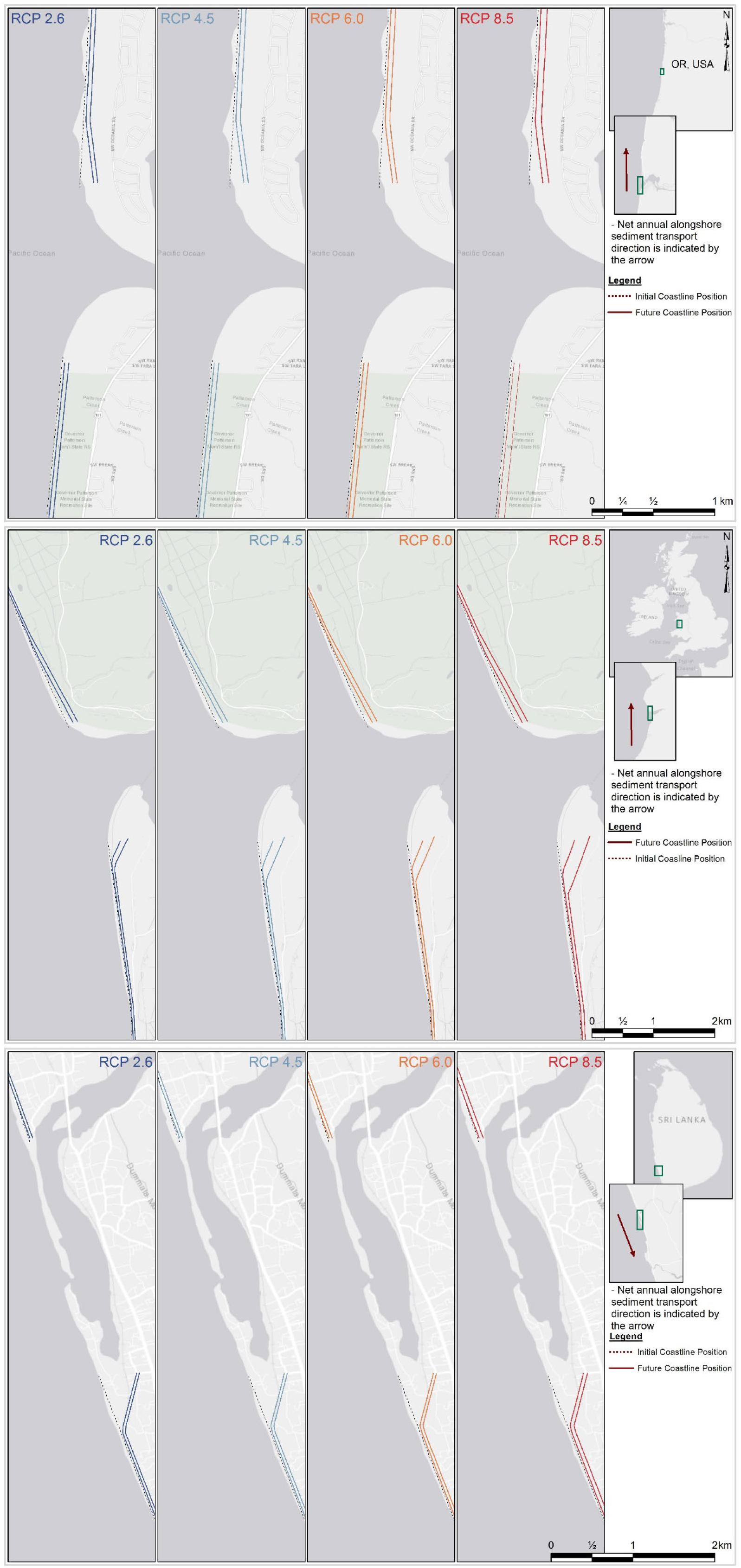
Figure 12. Projected changes of the inlet-affected coastline at the Alsea estuary (top), Dyfi estuary (middle), and Kalutara estuary (bottom). The two solid lines in each subplot represent the final coastline position by 2060 and 2100 (in the same order, moving landward from the most seaward line). The dotted line in each subplot represents the initial (reference) coastline position.
At the Alsea estuary system, the sediment demand of the basin (ΔVT) acts as a sediment sink. Therefore, the estuary imports sediment from the adjacent coast. The magnitude of the sediment demand of the estuary (ΔVT) is smaller than that of the ambient longshore sediment transport capacity at the Alsea estuary system. Therefore, the down-drift coast at the Alsea estuary system will be subjected to an additional coastline recession due to the variation in ΔVT, on top of recession due to the Bruun effect. Figure 12 (top) shows that the coastal recession along the down-drift coast of the Alsea estuary may vary between 67 m (RCP 2.6) and 86 m (RCP 8.5) by 2100. The up-drift coast is only affected by the coastal recession due to Bruun effect and hence projected to be move landward by between 54 m (RCP 2.6) and 72 m (RCP 8.5) by 2100.
At the Dyfi estuary system also, ΔVT acts as a sediment sink, and hence sediment will be imported into the estuary from the adjacent coast. The magnitude of the sediment demand of the estuary (ΔVT) is larger than that of the ambient longshore sediment transport capacity at the Dyfi estuary system. Therefore, both the up- and down-drift coasts at the Dyfi estuary system will be subjected to additional coastline recessions (on top of that due to the Bruun effect) to satisfy the estuarine sediment demand. The extent of the additional down-drift coastal recession is constrained by the magnitude of LST. The additional up-drift coastal recession is equivalent to the magnitudinal difference between the estuarine sediment demand (i.e., ΔVT) and the LST capacity. The model results shown in Figure 12 (middle) indicate that the down-drift coast at the Dyfi estuary may move landward by between 75 m (RCP 2.6) and 92 m (RCP 8.5) by 2100. The recession along the up-drift coast is larger and projected to be between 95 m (RCP 2.6) and 152 m (RCP 8.5) by 2100.
The Kalutara estuary system is also projected to import sediment from its adjacent coast and hence acts as a sediment sink for all but the end-century period under RCP 8.5. The magnitude of the sediment demand from the estuary is less than the current longshore sediment transport capacity at the inlet. Therefore, the down-drift coast will experience additional coastal recession driven by ΔVT, on top of that due to the Bruun effect. Under RCP 8.5, the fluvial sediment supply to the estuary increases during the 2080−2100 period, which results in a net positive ΔVT during this period. Thus, the Kalutara estuary system acts as a sediment source during this period under RCP 8.5. Therefore, the down-drift coast at Kalutara estuary is projected to prograde after 2080 under RCP 8.5 as sediment is exported by the estuary to the coast. However, this coastline progradation is less than the projected coastline recession due to the Bruun effect over the same period. Consequently, the cumulative effect of these two opposing contributions results in a net coastline recession along the down-drift coast. The up-drift coast is only affected by the coastline recession due to the Bruun effect. The model results [Figure 12 (bottom)] indicate that the down-drift coast at the Kalutara inlet may erode by between 92 m (RCP 2.6) to 105 m (RCP 8.5) by 2100. The up-drift coast is projected to erode by between 50 m (RCP 2.6) to 67 m (RCP 8.5) by 2100.
To scrutinize the contribution of river catchments and estuarine processes to the projected coastline changes along the inlet-interrupted coasts, the maximum and minimum shoreline change projections obtained from G-SMIC is compared with the coastline recessions due to the Bruun rule only. This comparison (Table 2) illustrates that the Bruun rule only is always underestimating the potential shoreline recessions at the three case study locations. The minimum projections of G-SMIC at Alsea estuary system is about 24% larger than projections obtained from the Bruun rule only. The same comparison at Dyfi and Kalutara estuary shows that G-SMIC projections area 84% larger than coastal recession due to the Bruun rule only. The maximum shoreline change projections obtained by G-SMIC at the Alsea and Kalutara estuary systems are respectively 20 and 57% larger than the Bruun rule only projections. The maximum shoreline change projection obtained by G-SMIC at the Dyfi estuary systems is 134% larger than the Bruun rule only projections of shoreline change. These numbers illustrates the significance of incorporating catchment and estuarine processes when simulating the evolution of inlet-interrupted coasts.
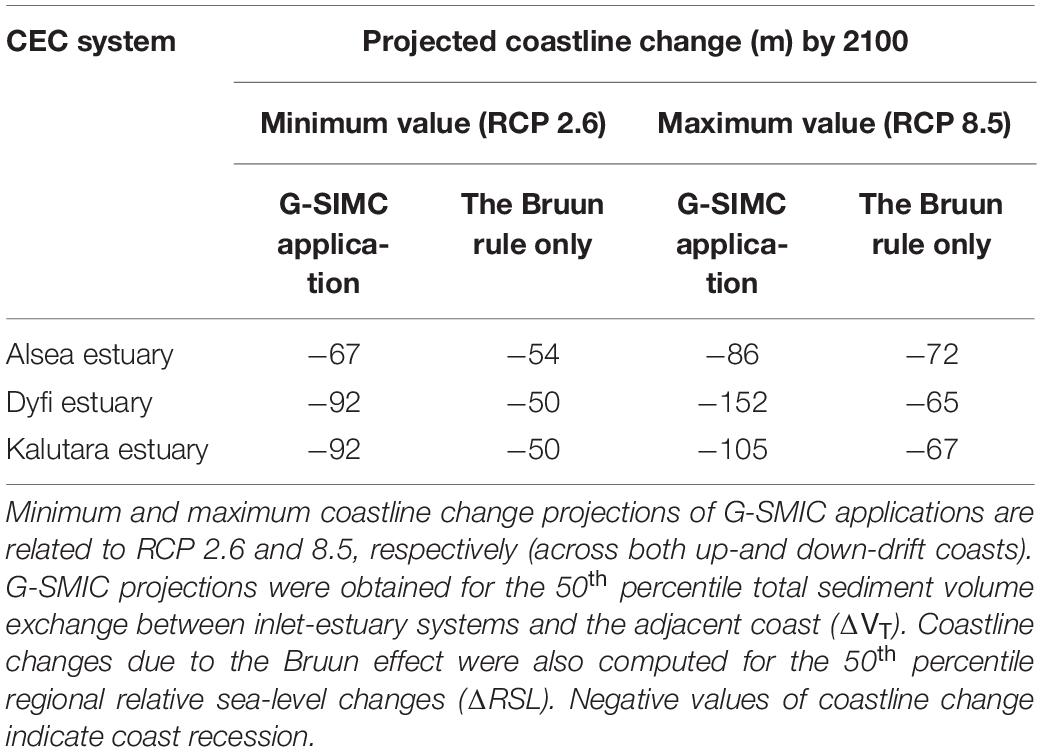
Table 2. Comparison of maximum and minimum coastline changes by 2100, obtained from G-SMIC applications and the Bruun rule only.
Discussion
The results of this study indicate that the variability in model inputs result in substantial uncertainties of the projected ΔVT by 2100. Results also show that future variation in total sediment volume exchange at tidal inlets (i.e., ΔVT) would be governed by one or two of its contributing components [i.e., basin infilling (ΔVBI), basin volume (ΔVBV), and fluvial sediment supply (ΔVFS)]. In this study, the focus was limited to quantifying the uncertainties associated with model inputs (i.e., only input uncertainties not model uncertainties). Specifically, this study takes into account the uncertainties in projections of temperature (T), river discharge (Q), regional relative sea-level change (ΔRSL), and human-induced erosion factor (Eh). Given that all GCM projections of T, Q and SLR are based on the Representative Concentration Pathways (RCPs) adopted by the IPCC, this study quantifies the differences in model projections obtained for the four IPCC RCPs.
However, it should be noted that the uncertainties quantified here are those associated with the single reduced-complexity model used. To quantify “model uncertainty” it would be necessary to derive projections from several different coastline change models (i.e., a multi-model ensemble). The result of such a multi-model ensemble is required to determine the likelihood ranges as adopted by the IPCC, which, as a precursor needs a high level of confidence (Cubasch et al., 2013). Therefore, the 10–90% ranges presented in the results only correspond to the output variability due to the model input uncertainties, and cannot be taken as an indication of likelihoods of the projections. As the results of the model are probabilistic, another interesting analysis that would be possible is the evaluation of the contribution of each input variable to the total variance of the projected coastline change. This could be achieved via the global sensitivity analysis approach (Sobol’, 2001). One application of this method with respect to coastline projection is presented by Le Cozannet et al. (2019).
Scrutinizing the projected model inputs indicate that annual mean temperature and cumulative river discharge have more significant uncertainties that the regional relative sea-level change projections. Therefore, variabilities associated with projections of T and Q are the major sources of model input uncertainties in this application. These are reflected in the projected uncertainties of ΔVT at the case study systems, as discussed in more detail below.
Projected sea-level rise has substantial implications on the behavior of all but the Kalutara inlet system, which has a relatively small estuary surface area. The overall variation of ΔVT at Kalutara estuary is governed by the change in fluvial sediment supply. Due to the uncertainties in key climatic model inputs (i.e., T and Q), the projected ΔVT at the Kalutara estuary system shows substantial variations, especially for RCP 8.5 during the end-century period. The deterministic projections of ΔVT for RCP 2.6 presented in Bamunawala et al. (2020) deviates (by about 15%) from the 50th percentile values of ΔVT of the probabilistic projections presented here. This deviation is due to the uncertainties associated with the model inputs (i.e., T and Q). The averaged ensemble values of T and Q used in the deterministic application of G-SMIC presented in Bamunawala et al. (2020) do not adequately account for the uncertainties associated with the GCM projections.
In addition to the estuarine sediment demand due to basin infilling, the Alsea estuary system is also significantly affected by the fluvial sediment supply. As a result, the projected ΔVT values at the Alsea estuary show considerable uncertainties for all RCPs, especially toward the end-century period (min-max range of 1.0 MCM for RCP 8.5). These uncertainties also arise from the variations associated with the model inputs (i.e., T and Q projections). However, due to the dominance of sea-level rise driven basin infilling in this case, these uncertainties are not as prominent as at the Kalutara estuary system. The deterministic projections of ΔVT for RCP 8.5 presented in Bamunawala et al. (2020) deviates (by about 30%) from the 50th percentile values of ΔVT of the probabilistic projections presented here. This deviation is due to the uncertainties associated with the model inputs (i.e., T and Q).
The Dyfi estuary system is dominated by the sea-level rise driven basin infilling. Therefore, the projected 50th percentile values of ΔVT at the Dyfi estuary system shows the best agreement with the deterministic model results presented by Bamunawala et al. (2020). This agreement illustrates the impact of the uncertainties associated with the climatic model inputs (i.e., T and Q) have on the projected ΔVTat CEC systems. The uncertainties of the projected ΔVT values at the Dyfi estuary follow the variability of ΔRSL and hence increases rapidly toward the end-century period for RCP 8.5.
The projected coastline changes at the case study sites by 2100 are compared with the model results presented in a global assessment of coastline change by Vousdoukas et al. (2020b) (Table 3). Here, only the projections made under RCP 8.5 are considered in this comparison. It should, however, be noted that the global assessment of sandy coastline variation presented by Vousdoukas et al. (2020b) does not consider the estuarine and watershed effects and incorporates a correction factor for Bruun effect-driven coastline recession. Therefore, the coastline change projections presented in this study will, by necessity, differ from the results presented in the global assessment of sandy shorelines by Vousdoukas et al. (2020b).
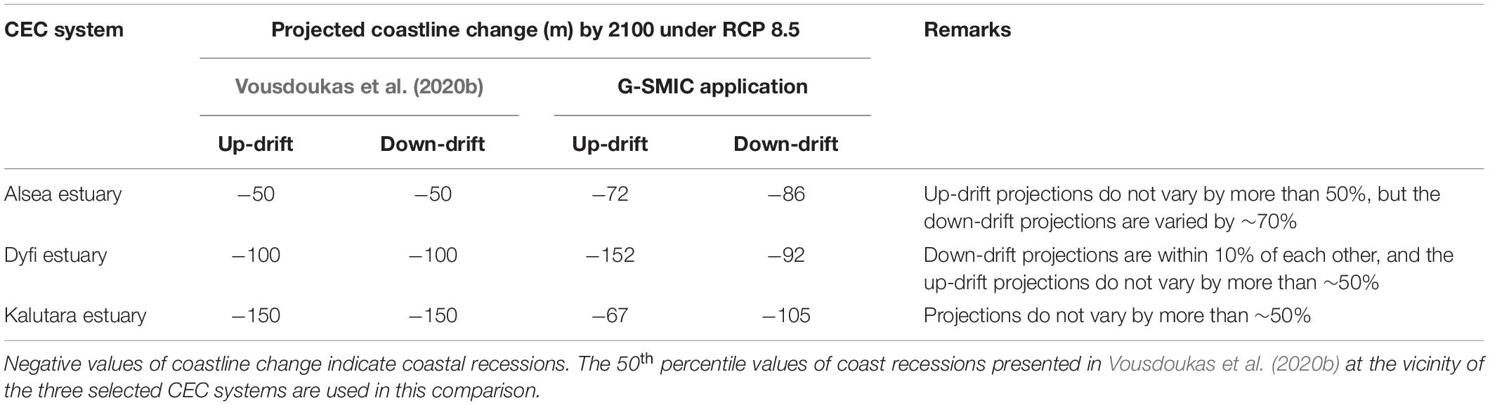
Table 3. Comparison of projected coastline change by 2100 with the results presented in Vousdoukas et al. (2020b) (for RCP 8.5).
It should be noted that because the shoreline changes presented here and by Bamunawala et al. (2020) are based on deviations from present (reference) river discharge and sediment input rates (and on SLR rates that are greater than present). These shoreline change rates are best interpreted as representing future deviations from present (reference) rates of shoreline change. For CEC systems with present rates of shoreline change that have a magnitude similar to the projected rates of shoreline change, based on the analysis presented here, final shoreline positions over the future time slices should be derived by superimposing the projected and reference rates of coastline change. For CEC systems in which projected rates of change based on this analysis are much larger than those under reference conditions, final shoreline positions will result mainly from the deviations from the present rates. The model hindcasts presented by Bamunawala et al. (2020) indicate that, for all the case study sites considered in this study, rates of projected coastline changes are of the same order of magnitude as the hindcast values. Therefore, in this study, all future coastline positions should be obtained by superimposing the hindcast rates of coastline changes presented by Bamunawala et al. (2020) with projected coastline changes shown in section “Projections of Coastline Change” and Figure 12.
It should also be noted that the coastline change projections presented here were obtained using the simplified one-line model presented in Bamunawala et al. (2020). This simplified coastline change model does not account for possible changes in longshore sediment transport rates and gradients therein due to future changes in wave conditions, local variations in coastline orientation (i.e., straight shoreline segments are assumed) or the presence of any coastal structures. The model also does not contain a built-in facility to apply any known limits to eroding sand from up- and down-drift coasts to fulfill estuarine sediment demand. Therefore, when applied along coasts with known limits for sand erodibility, an appropriate threshold should be considered. The model also does not consider the role that the deltas (when present) could play in distributing the exchange sediment volume (ΔVT). In general, in an inlet-estuary system containing significant ebb deltas with sediment that can be mobilized, part of the sediment demand from the estuary will be supplied from the ebb delta [e.g., Dissanayake et al. (2009, 2012)]. In such cases, these simplified model projections will overestimate coastline recession (i.e., pessimistic estimates). For a sediment exporting estuary system, a part of sediment received by the coast will contribute to the development of ebb delta. In such circumstances, model projections made by this simplified approach can be considered as optimistic projections (i.e., over-projection of coastline progradation). Therefore, these coastline change projections only provide first-order approximations of the long-term evolution of the coastline at the case study sites. Coupling the projected sediment volumes with a coastline change model that provides a more realistic representation of the shape and orientation of coastlines, such as the Coastline Evolution Model (CEM) (Ashton and Murray, 2006), the Coastal One-line Vector Evolution Model (COVE) (Hurst et al., 2015), or ShorelineS (Roelvink et al., 2020) will significantly enhance the quality of coastline change projections.
Conclusion
This manuscript presents the development and application of a reduced-complexity modeling technique that can probabilistically assess climate change-driven evolution of inlet-interrupted coasts at time scales of 50 to 100 years while taking into account the contributions from CEC systems in a holistic manner. The model represents the main physical processes that govern the variations of total sediment volume exchange between the estuary system (ΔVT) and the adjacent coast under the influence of climate change and anthropogenic activities. The probabilistic framework within which the model is applied here enabled the quantification of the uncertainties associated with the projected change in sediment volume exchange between the inlet-estuary systems and the adjacent coast and consequent coastline changes, arising from model input uncertainties. The model was applied to three case-study: the Alsea estuary (Oregon, United States), Dyfi estuary (Wales, United Kingdom), and Kalutara inlet (Sri Lanka) over the period 2020–2100.
Results obtained for the three case study sites showed that future variation in total sediment volume exchange at tidal inlets (i.e., ΔVT) could be governed by any of the contributing components [i.e., basin infilling (ΔVBI), basin volume (ΔVBV), and fluvial sediment supply (ΔVFS)] or combinations thereof. As such, the results of this study underlines the importance of taking into account all these processes when investigating future variations in the sediment budget at CEC systems.
Model projections showed that there are significant uncertainties associated with the sediment volume exchange between the estuary system (ΔVT) and inlet-interrupted coasts, especially for RCP 8.5 and toward the end-century period (2091–2100). These uncertainties arise mainly due to the intra-annual variabilities in projections of climatic variables (i.e., T and Q), and variations among the General Circulation Model (GCM) projections. Compared to the uncertainties in projections of T and Q, projections of regional relative sea-level change (ΔRSL) contain less variability over the 21st century. Inter-site differences between the projected 50th percentile values and the deterministic estimates of ΔVT illustrate the importance of adopting probabilistic modeling techniques to evaluate the long-term evolution of CEC systems.
Projections of coastline change at the three case study sites obtained with the 50th percentile projections of total sediment exchange volume (ΔVT) showed that accounting for basin infilling (ΔVBI), basin volume (ΔVBV), and fluvial sediment supply (ΔVFS) in computing coastline change at these inlet-interrupted coasts results in projections that are between 20% - 134% greater than the projections that would be obtained if only the Bruun effect were taken into account. This further emphasizes the need to consider the CEC systems in a holistic fashion when investigating coastline change along inlet-interrupted coasts.
Data Availability Statement
The raw data supporting the conclusions of this article will be made available by the authors, without undue reservation.
Author Contributions
JB, AD, AS, and RR conceived and designed the study. JB developed the model, carried out all model applications, and wrote the first draft of the manuscript. SM provided specific guidance on the catchment hydrology aspects of the study. TD provided specific guidance on the SMIC model adaptation and QA’d the new code. TS assisted with GCM data collection and catchment delineation. All authors provided feedback on the manuscript and contributed text.
Funding
This study is part of JB’s Ph.D. research which is supported by the Deltares Research Programme ‘Understanding System Dynamics; from River Basin to Coastal Zone’ and the AXA Research Fund. RR was supported by the AXA Research Fund and the Deltares Strategic Research Programme ‘Coastal and Offshore Engineering’.
Conflict of Interest
The authors declare that the research was conducted in the absence of any commercial or financial relationships that could be construed as a potential conflict of interest.
The reviewer AD’A declared a past co-authorship with one of the authors AM to the handling editor.
Acknowledgments
Last of the Wild Project, Global Human Footprint, Version 2 data were developed by the Wildlife Conservation Society – WCS and the Center for International Earth Science Information Network (CIESIN), Columbia University and were obtained from the NASA Socioeconomic Data and Applications Center (SEDAC) at http://dx.doi.org/10.7927/H4M61H5F. Accessed 1 October 2015. Any use of trade, firm, or product names is for descriptive purposes only and does not imply endorsement by the United States Government.
Supplementary Material
The Supplementary Material for this article can be found online at: https://www.frontiersin.org/articles/10.3389/fmars.2020.579203/full#supplementary-material
References
Anthony, E. J., Brunier, G., Besset, M., Goichot, M., Dussouillez, P., and Nguyen, V. L. (2015). Linking rapid erosion of the Mekong River delta to human activities. Sci. Rep. 5:14745. doi: 10.1038/srep14745
Ashton, A. D., and Murray, A. B. (2006). High-angle wave instability and emergent shoreline shapes: 1. Modeling of sand waves, flying spits, and capes. J. Geophys. Res. Earth Surf. 111:F04011. doi: 10.1029/2005JF000422
Aubrey, D. G., and Weishar, L. (eds) (1988). Hydrodynamics and Sediment Dynamics of Tidal Inlets. New York, NY: Springer, doi: 10.1007/978-1-4757-4057-8
Balthazar, V., Vanacker, V., Girma, A., Poesen, J., and Golla, S. (2013). Human impact on sediment fluxes within the blue nile and atbara river basins. Geomorphology 180–181, 231–241. doi: 10.1016/j.geomorph.2012.10.013
Bamunawala, J., Dastgheib, A., Ranasinghe, R., van der Spek, A., Maskey, S., Murray, A. B., et al. (2020). A holistic modeling approach to project the evolution of inlet-interrupted coastlines over the 21st century. Front. Mar. Sci. 7:542. doi: 10.3389/fmars.2020.00542
Bamunawala, J., Maskey, S., Duong, T., and van der Spek, A. (2018a). Significance of fluvial sediment supply in coastline modelling at tidal inlets. J. Mar. Sci. Eng. 6:79. doi: 10.3390/jmse6030079
Bamunawala, J., Ranasinghe, R., van der Spek, A., Maskey, S., and Udo, K. (2018b). Assessing future coastline change in the vicinity of tidal inlets via reduced complexity modelling. J. Coast. Res. 85, 636–640. doi: 10.2112/SI85-128.1
Besset, M., Anthony, E. J., and Bouchette, F. (2019). Multi-decadal variations in delta shorelines and their relationship to river sediment supply: an assessment and review. Earth Sci. Rev. 193, 199–219. doi: 10.1016/j.earscirev.2019.04.018
Bosello, F., Nicholls, R. J., Richards, J., Roson, R., and Tol, R. S. J. (2012). Economic impacts of climate change in Europe: sea-level rise. Clim. Change 112, 63–81. doi: 10.1007/s10584-011-0340-1
Brown, S., Nicholls, R. J., Hanson, S., Brundrit, G., Dearing, J. A., Dickson, M. E., et al. (2014). Shifting perspectives on coastal impacts and adaptation. Nat. Clim. Chang. 4, 752–755. doi: 10.1038/nclimate2344
CSIRO, and Bureau of Meteorology (2015). Climate Change in Australia Information for Australia’s Natural Resource Management Regions: Technical Report. Australia: CSIRO and Bureau of Meteorology.
Cubasch, U., Wuebbles, D., Chen, D., Facchini, M. C., Frame, D., Mahowald, N., et al. (2013). “‘Introduction’,” in Climate Change 2013: The Physical Science Basis. Contribution of Working Group I to the Fifth Assessment Report of the Intergovernmental Panel on Climate Change, eds T. F. Stocker, D. Qin, G.-K. Plattner, M. Tignor, S. K. Allen, J. Boschung, et al. (Cambridge: Cambridge University Press).
Dastgheib, A., Jongejan, R., Wickramanayake, M., and Ranasinghe, R. (2018). Regional scale risk-informed land-use planning using probabilistic coastline recession modelling and economical optimisation: east coast of Sri Lanka. J. Mar. Sci. Eng. 6:120. doi: 10.3390/jmse6040120
Dean, R. G. G., and Houston, J. R. R. (2016). Determining shoreline response to sea level rise. Coast. Eng. 114, 1–8. doi: 10.1016/j.coastaleng.2016.03.009
Dissanayake, D. M. P. K., Ranasinghe, R., and Roelvink, J. A. (2012). The morphological response of large tidal inlet/basin systems to relative sea level rise. Clim. Change 113, 253–276. doi: 10.1007/s10584-012-0402-z
Dissanayake, D. M. P. K., Roelvink, J. A., and van der Wegen, M. (2009). Modelled channel patterns in a schematized tidal inlet. Coast. Eng. 56, 1069–1083. doi: 10.1016/j.coastaleng.2009.08.008
Dunn, F. E., Darby, S. E., Nicholls, R. J., Cohen, S., Zarfl, C., and Fekete, B. M. (2019). Projections of declining fluvial sediment delivery to major deltas worldwide in response to climate change and anthropogenic stress. Environ. Res. Lett. 14:84034. doi: 10.1088/1748-9326/ab304e
Dunn, F. E., Nicholls, R. J., Darby, S. E., Cohen, S., Zarfl, C., and Fekete, B. M. (2018). Projections of historical and 21st century fluvial sediment delivery to the Ganges-Brahmaputra-Meghna, Mahanadi, and Volta deltas. Sci. Total Environ. 642, 105–116. doi: 10.1016/j.scitotenv.2018.06.006
Duong, T. M., Ranasinghe, R., Walstra, D., and Roelvink, D. (2016). Assessing climate change impacts on the stability of small tidal inlet systems: why and how? Earth Sci. Rev. 154, 369–380. doi: 10.1016/j.earscirev.2015.12.001
FitzGerald, D. M., Fenster, M. S., Argow, B. A., and Buynevich, I. V. (2008). Coastal impacts due to sea-level rise. Annu. Rev. Earth Planet. Sci. 36, 601–647. doi: 10.1146/annurev.earth.35.031306.140139
FitzGerald, D. M., Georgiou, I., and Miner, M. (2015). “‘Estuaries and tidal inlets’,” in Coastal Environments and Global Change, eds G. Masselink and R. Gehrels (Chichester: John Wiley & Sons Ltd), 268–298. doi: 10.1002/9781119117261.ch12
Hallegatte, S., Green, C., Nicholls, R. J., and Corfee-Morlot, J. (2013). Future flood losses in major coastal cities. Nat. Clim. Chang. 3:802. doi: 10.1038/nclimate1979
Hegerl, G. C., Black, E., Allan, R. P., Ingram, W. J., Polson, D., Trenberth, K. E., et al. (2015). Challenges in quantifying changes in the global water cycle. Bull. Am. Meteorol. Soc. 96, 1097–1115. doi: 10.1175/BAMS-D-13-00212.1
Hinkel, J., Nicholls, R. J., Tol, R. S. J., Wang, Z. B., Hamilton, J. M., Boot, G., et al. (2013). A global analysis of erosion of sandy beaches and sea-level rise: an application of DIVA. Glob. Planet. Change 111, 150–158. doi: 10.1016/j.gloplacha.2013.09.002
Hugo, G. (2011). Future demographic change and its interactions with migration and climate change. Glob. Environ. Chang. 21, S21–S33. doi: 10.1016/j.gloenvcha.2011.09.008
Hurst, M. D., Barkwith, A., Ellis, M. A., Thomas, C. W., and Murray, A. B. (2015). Exploring the sensitivities of crenulate bay shorelines to wave climates using a new vector-based one-line model. J. Geophys. Res. Earth Surf. 120, 2586–2608. doi: 10.1002/2015JF003704
Jongejan, R., Ranasinghe, R., Wainwright, D., Callaghan, D. P., and Reyns, J. (2016). Drawing the line on coastline recession risk. Ocean Coast. Manag. 122, 87–94. doi: 10.1016/j.ocecoaman.2016.01.006
Kirezci, E., Young, I. R., Ranasinghe, R., Muis, S., Nicholls, R. J., Lincke, D., et al. (2020). Projections of global-scale extreme sea levels and resulting episodic coastal flooding over the 21st Century. Sci. Rep. 10:11629.
Le Cozannet, G., Bulteau, T., Castelle, B., Ranasinghe, R., Wöppelmann, G., Rohmer, J., et al. (2019). Quantifying uncertainties of sandy shoreline change projections as sea level rises. Sci. Rep. 9:42. doi: 10.1038/s41598-018-37017-4
Le Cozannet, G., Nicholls, J. R., Hinkel, J., Sweet, V. W., McInnes, L. K., Van de Wal, S. W. R., et al. (2017). Sea level change and coastal climate services: the way forward. J. Mar. Sci. Eng. 5:49. doi: 10.3390/jmse5040049
Luijendijk, A., Hagenaars, G., Ranasinghe, R., Baart, F., Donchyts, G., and Aarninkhof, S. (2018). The State of the World’s Beaches. Sci. Rep. 8:6641. doi: 10.1038/s41598-018-24630-6
McGranahan, G., Balk, D., and Anderson, B. (2007). The rising tide: assessing the risks of climate change and human settlements in low elevation coastal zones. Environ. Urban. 19, 17–37. doi: 10.1177/0956247807076960
McSweeney, S. L., Kennedy, D. M., Rutherfurd, I. D., and Stout, J. C. (2017). Intermittently Closed/Open lakes and lagoons: their global distribution and boundary conditions. Geomorphology 292, 142–152. doi: 10.1016/j.geomorph.2017.04.022
Mehvar, A., Dastgheib, A., and Ranasinghe, R. (2016). Relative Sea Level Rise Scenarios: Central Coast of Bangladesh. Delft: Delft University of Technology.
Merkens, J.-L., Reimann, L., Hinkel, J., and Vafeidis, A. T. (2016). Gridded population projections for the coastal zone under the shared socioeconomic pathways. Glob. Planet. Change 145, 57–66. doi: 10.1016/j.gloplacha.2016.08.009
Murray, A. B. (2007). Reducing model complexity for explanation and prediction. Geomorphology 90, 178–191. doi: 10.1016/j.geomorph.2006.10.020
Murray, A. B., and Moore, L. J. (2018). “‘Geometric constraints on long-term barrier migration: from simple to surprising BT’,” in Barrier Dynamics and Response to Changing Climate, eds L. J. Moore and A. B. Murray (Cham: Springer International Publishing), 211–241. doi: 10.1007/978-3-319-68086-6_7
Neumann, B., Vafeidis, A. T., Zimmermann, J., and Nicholls, R. J. (2015). Future coastal population growth and exposure to sea-level rise and coastal flooding - a global assessment. PLoS One 10:e0118571. doi: 10.1371/journal.pone.0118571
Nicholls, R. J., Hanson, S. E., Lowe, J. A., Warrick, R. A., Lu, X., Long, A. J., et al. (2011). Constructing Sea-Level Scenarios for Impact and Adaptation Assessment of Coastal Area: A Guidance Document. Supporting Material, Intergovernmental Panel on Climate Change Task Group on Data and Scenario Support for Impact and Climate Analysis. Geneva: IPCC.
Overeem, I., and Syvitski, J. P. M. (2009). Dynamics and Vulnerability of Delta Systems. LOICZ Reports & Studies No. 35. Geesthacht: GKSS Research Center.
Palmer, M. A., Liermann, C. A. R., Nilsson, C., Flörke, M., Alcamo, J., Lake, P. S., et al. (2008). Climate change and the world’s river basins: anticipating management Options. Front. Ecol. Environ. 6:81–89. doi: 10.1890/060148
Prahl, B. F., Boettle, M., Costa, L., Kropp, J. P., and Rybski, D. (2018). Damage and protection cost curves for coastal floods within the 600 largest European cities. Sci. Data 5:180034. doi: 10.1038/sdata.2018.34
Rahmstorf, S. (2007). A semi-empirical approach to projecting future sea-level rise. Science 315, 368–370. doi: 10.1126/science.1135456
Ranasinghe, R. (2016). Assessing climate change impacts on open sandy coasts: a review. Earth-Science Rev. 160, 320–332. doi: 10.1016/j.earscirev.2016.07.011
Ranasinghe, R. (2020). On the need for a new generation of coastal change models for the 21st century. Sci. Rep. 10:2010. doi: 10.1038/s41598-020-58376-x
Ranasinghe, R., Callaghan, D., and Stive, M. J. F. (2012). Estimating coastal recession due to sea level rise: beyond the Bruun rule. Clim. Change 110, 561–574. doi: 10.1007/s10584-011-0107-8
Ranasinghe, R., Duong, T. M., Uhlenbrook, S., Roelvink, D., and Stive, M. (2013). Climate-change impact assessment for inlet-interrupted coastlines. Nat. Clim. Chang. 3, 83–87. doi: 10.1038/nclimate1664
Ranasinghe, R., and Stive, M. J. F. (2009). Rising seas and retreating coastlines. Clim. Change 97:465. doi: 10.1007/s10584-009-9593-3
Ranasinghe, R., Wu, C. S., Conallin, J., Duong, T. M., and Anthony, E. J. (2019). Disentangling the relative impacts of climate change and human activities on fluvial sediment supply to the coast by the world’s large rivers: Pearl River Basin. China. Sci. Rep. 9:9236. doi: 10.1038/s41598-019-45442-2
Roelvink, D., Huisman, B., Elghandour, A., Ghonim, M., and Reyns, J. (2020). Efficient modeling of complex sandy coastal evolution at monthly to century time scales. Front. Mar. Sci. 7:535. doi: 10.3389/fmars.2020.00535
Sobol’, I. M. (2001). Global sensitivity indices for nonlinear mathematical models and their Monte Carlo estimates. Math. Comput. Simul. 55, 271–280. doi: 10.1016/S0378-4754(00)00270-6
Spencer, T., Schuerch, M., Nicholls, R. J., Hinkel, J., Lincke, D., Vafeidis, A. T., et al. (2016). Global coastal wetland change under sea-level rise and related stresses: the DIVA wetland change model. Glob. Planet. Change 139, 15–30. doi: 10.1016/j.gloplacha.2015.12.018
Stive, M. J. F. (2004). How important is global warming for coastal erosion? Clim. Change 64, 27–39. doi: 10.1023/B:CLIM.0000024785.91858.1d
Stive, M. J. F., Capobianco, M., Wang, Z. B., Ruol, P., and Buijsman, M. C. (1998). “‘Morphodynamics of a tidal lagoon and the adjacent Coast’,” in Physics of Estuaries and Coastal Seas, eds J. Dronkers and M. Scheffers (Rotterdam: A. A. Balkema), 397–407.
Stive, M. J. F., Roelvink, J. A., and de Vriend, H. J. (1990). “Large-scale coastal evolution concept,” in Proceedings of the 22nd International Conference on Coastal Engineering, (Delft: Delft University), 1962–1974. doi: 10.1061/9780872627765.150
Stocker, T. F., Qin, D., Plattner, G.-K., Alexander, L. V., Allen, S. K., Bindoff, N. L., et al. (2013a). “‘Technical summary’,” in Climate Change 2013: The Physical Science Basis. Contribution of Working Group I to the Fifth Assessment Report of the Intergovernmental Panel on Climate Change, eds T. F. Stocker, D. Qin, G.-K. Plattner, M. Tignor, S. K. Allen, J. Boschung, et al. (Cambridge: Cambridge University Press).
Stocker, T. F., Qin, D., Plattner, G.-K., Tignor, M., Allen, S. K., and Boschung, J., et al. (eds) (2013b). “IPCC, 2013: summary for policymakers,” in Climate Change 2013: The Physical Science Basis. Contribution of Working Group I to the 5th Assessment Report of the Intergovernmental Panel on Climate Change, (Cambridge: Cambridge University Press).
Syvitski, J. P. M. (2005). Impact of humans on the flux of terrestrial sediment to the global coastal Ocean. Science 308, 376–380. doi: 10.1126/science.1109454
Syvitski, J. P. M., and Kettner, A. J. (2008). “Scaling sediment flux across landscapes,” in Sediment Dynamics in Changing Environments, eds J. Schmidt, T. Cochrane, C. Phillips, S. Elliot, T. Davies, and L. Basher (Christchurch: IAHS Publications), 149–156.
Syvitski, J. P. M., Kettner, A. J., Overeem, I., Hutton, E. W. H., Hannon, M. T., Brakenridge, G. R., et al. (2009). Sinking deltas due to human activities. Nat. Geosci. 2, 681–686. doi: 10.1038/ngeo629
Syvitski, J. P. M., and Milliman, J. D. (2007). Geology, geography, and humans battle for dominance over the delivery of fluvial sediment to the Coastal Ocean. J. Geol. 115, 1–19. doi: 10.1086/509246
Taylor, K., Ronald, S., and Meehl, G. (2011). An overview of CMIP5 and the experiment design. Bull. Am. Meteorol. Soc. 93, 485–498. doi: 10.1175/BAMS-D-11-00094.1
Toimil, A., Losada, I. J., Camus, P., and Díaz-Simal, P. (2017). Managing coastal erosion under climate change at the regional scale. Coast. Eng. 128, 106–122. doi: 10.1016/j.coastaleng.2017.08.004
Trenberth, K. E., Smith, L., Qian, T., Dai, A., and Fasullo, J. (2007). Estimates of the global water budget and its annual cycle using observational and model Data. J. Hydrometeorol. 8, 758–769. doi: 10.1175/JHM600.1
Vafeidis, A., Neumann, B., Zimmermann, J., and Nicholls, R. J. (2011). MR9: Analysis of Land Area and Population in the Low-Elevation Coastal Zone (LECZ). London: The Government Office for Science, 172.
van Maanen, B., Nicholls, R. J., French, J. R., Barkwith, A., Bonaldo, D., Burningham, H., et al. (2016). Simulating mesoscale coastal evolution for decadal coastal management: a new framework integrating multiple, complementary modelling approaches. Geomorphology 256, 68–80. doi: 10.1016/j.geomorph.2015.10.026
Veerbeek, W. (2017). Estimating the Impacts of Urban Growth on Future Flood Risk: A Comparative Study. Leiden: CRC Press/Balkema – Taylor & Francis Group. doi: 10.1016/j.geomorph.2015.10.026
Vörösmarty, C. J., Meybeck, M., Fekete, B., Sharma, K., Green, P., and Syvitski, J. P. M. (2003). Anthropogenic sediment retention: major global impact from registered river impoundments. Glob. Planet. Change 39, 169–190. doi: 10.1016/S0921-8181(03)00023-27
Vousdoukas, M. I., Mentaschi, L., Hinkel, J., Ward, P. J., Mongelli, I., Ciscar, J.-C., et al. (2020a). Economic motivation for raising coastal flood defenses in Europe. Nat. Commun. 11:2119. doi: 10.1038/s41467-020-15665-3
Vousdoukas, M. I., Ranasinghe, R., Mentaschi, L., Plomaritis, T. A., Athanasiou, P., Luijendijk, A., et al. (2020b). Sandy coastlines under threat of erosion. Nat. Clim. Chang. 10, 260–263. doi: 10.1038/s41558-020-0697-0
Vousdoukas, M. I., Mentaschi, L., Voukouvalas, E., Bianchi, A., Dottori, F., and Feyen, L. (2018). Climatic and socioeconomic controls of future coastal flood risk in Europe. Nat. Clim. Chang. 8, 776–780. doi: 10.1038/s41558-018-0260-4
Wolinsky, M. A., and Murray, A. B. (2009). A unifying framework for shoreline migration: 2. Application to wave-dominated coasts. J. Geophys. Res. Earth Surf. 114:F01009. doi: 10.1029/2007JF000856
Wong, P. P., Losada, I. J., Gattuso, J.-P., Hinkel, J., Khattabi, A., McInnes, K. L., et al. (2014). “‘Coastal systems and low-lying areas’,” in Climate Change 2014: Impacts, Adaptation, and Vulnerability. Part A: Global and Sectoral Aspects. Contribution of Working Group II to the Fifth Assessment Report of the Intergovernmental Panel on Climate Change, eds C. B. Field, V. R. Barros, D. J. Dokken, K. J. Mach, M. D. Mastrandrea, T. E. Bilir, et al. (Cambridge: Cambridge University Press), 361–409.
Keywords: catchment-estuary-coastal systems, climate change, inlet-interrupted coasts, input uncertainties, probabilistic model
Citation: Bamunawala J, Dastgheib A, Ranasinghe R, van der Spek A, Maskey S, Murray AB, Barnard PL, Duong TM and Sirisena TAJG (2020) Probabilistic Application of an Integrated Catchment-Estuary-Coastal System Model to Assess the Evolution of Inlet-Interrupted Coasts Over the 21st Century. Front. Mar. Sci. 7:579203. doi: 10.3389/fmars.2020.579203
Received: 01 July 2020; Accepted: 23 November 2020;
Published: 16 December 2020.
Edited by:
Zeng Zhou, Hohai University, ChinaReviewed by:
Pushpa Dissanayake, University of Kiel, GermanyAndrea D’Alpaos, University of Padua, Italy
Copyright © 2020 Bamunawala, Dastgheib, Ranasinghe, van der Spek, Maskey, Murray, Barnard, Duong and Sirisena. This is an open-access article distributed under the terms of the Creative Commons Attribution License (CC BY). The use, distribution or reproduction in other forums is permitted, provided the original author(s) and the copyright owner(s) are credited and that the original publication in this journal is cited, in accordance with accepted academic practice. No use, distribution or reproduction is permitted which does not comply with these terms.
*Correspondence: Janaka Bamunawala, ai5iYW11bmF3YWxhQGdtYWlsLmNvbQ==