Acoustic Detection of Krill Scattering Layer in the Terra Nova Bay Polynya, Antarctica

Krill play a crucial role in the transfer of energy in the marine food web, connecting primary producers and the upper trophic levels in the Terra Nova Bay polynya (TNBP), which is part of the Ross Sea marine protected area. Despite the substantial ecological importance of krill, there are few studies on their distribution and abundance in the TNBP. An acoustic survey was conducted on 7–14 January 2019 in the TNBP, Ross Sea, using a Simrad EK60 echosounder (38 and 120 kHz) aboard the icebreaker RV Araon. The most commonly used range of the difference of the mean volume backscattering strength (MVBS) (2–16 dB) was applied to distinguish krill. The acoustic data (120 kHz) were extracted to examine the krill distribution characteristics. The study area was divided into low-value areas and high-value areas based on the third quartile of the nautical area scattering coefficient. The results showed that the krill aggregations were distributed in three layers at depths of 0–30 m, 70–110 m, and 270–300 m. The interpolated environmental parameters associated with the backscattering strength were compared. High-value areas of krill coincided with relatively low temperature, low salinity, and high chlorophyll, although very weak correlations were found. The primary goal of this study was to understand the vertical and horizontal distributions of krill acoustic biomass and to relate the observed patterns to the dominant environmental conditions.

Introduction

Krill (euphausiids) are considered keystone species in the Southern Ocean marine ecosystem (Atkinson et al., 2004) and in commercial fisheries (Nicol et al., 2012). They also play an important role in the biogeochemical carbon cycle (Belcher et al., 2017; Cavan et al., 2019). Krill research has been intensively conducted in the pelagic and slope waters of the Southern Ocean (Nicol, 2006). However, our understanding of the krill distribution on the Antarctic continental shelf is much more limited than that in the open ocean because sea ice restricts accessibility.

The Ross Sea continental shelf is the most productive region in the Southern Ocean (Arrigo et al., 2008; Smith et al., 2014) and produces massive plankton and krill blooms that support huge numbers of fish, seals, penguins, birds, and whales (Ainley, 2010; Ballard et al., 2011). The prevalence of mid- to high-tropic levels in the Ross Sea habitat can result in extraordinarily high primary production, amounting to approximately 28% of the total primary production of the Southern Ocean (Arrigo et al., 1998, 2008; Ballard et al., 2011). In 2017, the Ross Sea became the world’s largest marine protected area. As a result, marine life resources in this region will be protected from heavy fishing and shipping pressure for the next 35 years. The Convention for the Conservation of Antarctic Marine Living Resources (CCAMLR) has strongly encouraged scientific research to protect and assess the Ross Sea marine ecosystem now and in the future.

Coastal polynyas are controlled by physical processes, such as wind, glaciers, and heat (Zwally et al., 1985; Van Woert et al., 2001; Arrigo and Van Dijken, 2003; Rusciano et al., 2013). Such areas enhance phytoplankton biomass growth (Gradinger and Baumann, 1991; Von Quillfeldt, 1997; Arrigo et al., 2000), primary production (Arrigo et al., 2000), and the rates of particle flux (Cooper et al., 2002) by fecal pellet production and aggregation during phytoplankton blooms. As a result of their persistent high productivity, coastal polynyas are also a critical habitat for microzooplankton (Li et al., 2001), copepods (Hosie and Cochran, 1994; Li et al., 2001), krill (Pakhomov et al., 2002; La et al., 2015b), and salps (Li et al., 2001; Pakhomov et al., 2002). A high density of krill has been found in coastal polynyas (La et al., 2015b). Thus, coastal polynyas are ideal sites to examine how a coastal marine ecosystem responds to environmental variations in the Southern Ocean (La et al., 2019).

The Terra Nova Bay polynya (TNBP) is a part of both the marine protected area and the Antarctic Special Protected Area (n.161) in the western Ross Sea (Mangoni et al., 2019). The TNBP is governed by katabatic winds that drive older sea ice offshore, allowing the development of new frazil ice (Van Woert et al., 2001; Arrigo and Van Dijken, 2003) and the presence of glacier ice that redirects sea ice away from the coast (Massom et al., 2001). This region persists during wintertime (Bromwich and Kurtz, 1984). The TNBP habitat in late spring and summer is often dominated by diatoms associated with a highly stratified water column due to the melting of a large amount of sea ice (Arrigo and Van Dijken, 2003), while Phaeocystis antarctica dominates more well-mixed waters (Wright and van den Enden, 2000). Diatoms and P. antarctica, two dominant phytoplankton species, coexist little on spatial and temporal scales after a bloom commences, representing competitive exclusion (Arrigo et al., 2000). The variation in phytoplankton community structures could affect the distribution pattern of dominant krill species because krill can have different biochemical compositions, diets, and habitat preferences (Bottino, 1974; Azzali et al., 2006).

Antarctic krill (Euphausia superba) and ice krill (E. crystallorophias) are two dominant species that connect primary producers to the upper trophic levels in the Ross Sea (Ainley et al., 2006; Smith et al., 2007; Pinkerton and Bradford-Grieve, 2014; Davis et al., 2017). Antarctic krill are dominant in the northern and northwestern areas of the Ross Sea. They are concentrated along the northwestern shelf break, and their habitat is characterized by deep (> 1,000 m) bottom depths, warm water, decreased sea ice, and proximity to the shelf break (Davis et al., 2017). Ice krill replace Antarctic krill in the southern high-latitude coastal zones (Sala et al., 2002; Azzali et al., 2006) and are predominant in southwestern locations, in proximity to the coast, and in cold water in the Ross Sea (Davis et al., 2017). Ice krill are known as the principal food source for many vertebrates in the high-latitude Antarctic food web (Whitehead et al., 1990; Pakhomov and Perissinotto, 1996). Recent studies have shown that high densities of ice krill are found in high-latitude coastal polynyas, such as those in Prydz Bay and the Amundsen Sea (La et al., 2015b). High densities of ice krill have been observed during summer within the Amundsen Sea coastal polynya, which is known to be one of the most productive regions in the Southern Ocean (Arrigo and Van Dijken, 2003). Plentiful summer food and the open water area could be key factors for the presence of high ice krill densities within this coastal polynya. Despite the great ecological importance and abundance of both Antarctic krill and ice krill, their presence and distribution are not well known in the coastal region around the Antarctic continent. Surprisingly, little is known about the spatial distribution of krill biomass in the TNBP and their role in food web dynamics.

It is essential to observe and assess the current spatial distribution of krill because understanding their response to environmental change and energy transfer within the food web depends on knowledge of the krill distribution. Spatial and temporal information on krill biomass can be obtained from scientific surveys with nets or acoustics, predator studies, and data from commercial fisheries. Each method has its advantages and disadvantages, and the methods are generally complementary (Atkinson et al., 2012). Net sampling, which has been a traditional method since the 1920s, provides important snapshots of marine ecosystems, but it suffers from the issues of avoidance, differing catchability, distribution heterogeneity, and a limited ability to provide a broad context (Kasatkina et al., 2004). Acoustics have been widely used to investigate the distribution, stock estimates, and ecology of krill in the Southern Ocean (Fielding et al., 2014; La et al., 2015a,b), although such studies are unable to provide species identification and suffer from acoustic dead zones. Krill monitoring programs were initiated using net and acoustic methods in the late 1980s (Reiss et al., 2008; Fielding et al., 2014; Krafft et al., 2016). In the TNBP, a few studies have been conducted to understand the spatial distribution of krill biomass using either acoustic-based methods (Azzali and Kalinowski, 2000; Azzali et al., 2006; Leonori et al., 2017) or net sampling (Sala et al., 2002; Guglielmo et al., 2009; Smith et al., 2017).

Here, we present a recent survey of the spatial variability of krill distributions during the austral summer of 2019 in the TNBP. Krill biomass was determined by acoustic-based measurements of sound-scattering layers; this method has been used for a long time to monitor the spatial and temporal variability in krill acoustic biomass in the Southern Ocean (Foote and Stanton, 2000; Fielding et al., 2014; La et al., 2015a,b). The primary goal of this study was to understand the vertical and horizontal distribution of krill and to relate the observed patterns to the dominant environmental conditions.

Materials and Methods

Data Collection

Acoustic data were collected using a scientific echosounder (EK60 split beam, Simrad) with operating frequencies of 38 and 120 kHz aboard the icebreaker RV Araon. GPS data were input into the echosounder to provide position information (latitude and longitude). The 38- and 120-kHz transducers were calibrated under calm weather conditions at 74°41′S and 164°9′E off the Jangbogo research station according to standard procedures (Foote et al., 1987) on 12 January 2019 (Table 1). The survey was conducted on 7–14 January 2019 in the TNBP, Ross Sea, Antarctica (Figure 1). A coastal polynya was visible by the northern side of the Drygalski ice tongue and the margin of the Nansen ice sheet. While recording acoustic data, the water temperature and salinity were measured underway at a depth of 7 m using a thermosalinograph (SBE45), and the fluorescence was measured using a Turner Designs 10-AU at the same depth. In fact, the two systems were not calibrated. Acoustic data were recorded in the water column and analyzed up to a depth of 300 m. To examine the relationship between the acoustic data and the environmental attributes, environmental data were required up to 300 m. Thus, environmental data from the water surface to a depth of 300 m in the study area were retrieved from the Copernicus Marine Environment Monitoring Service (CMEMS; Copernicus Marine Service, 2020). For temperature and salinity data, the NEMO 3.1 model was employed with a spatial resolution of 0.083° × 0.083° using assimilated observations such as the CMEMS operational sea surface temperature and the ice analysis (OSTIA) and sea surface temperature (SST), the in situ profile from the CMEMS database, and others. The OSTIA SST is produced from satellite and in situ observation data. The in situ profile from CMEMS included Argo profiling floats, gliders, bathythermographs, and other sources. Detailed information on the NEMO model can be found in Madec et al. (1988). The observed temperature data were averaged hourly or daily or monthly based on the source of the observation system. The observed salinity data were averaged daily or monthly. The location for extracting the temperature and salinity data was set as 74–76°S and 160–170°E, and the time was from 7 to 14 January 2019, with a water depth range of 0–300 m. The temperature and salinity outputs were recorded daily with vertical resolution of 1–17.4 m from the water surface to 100 m and that of 36–52 m from 200 to 300 m. For chlorophyll (mg/m³), the Pelagic Interactions Scheme for Carbon and Ecosystem Studies (PISCES) biogeochemical model was used, with a spatial resolution of 0.25°× 0.25° and various sensors such as the sea-viewing wide field-of-view sensor (SeaWiFS), the medium resolution imaging spectrometer (MERIS), the moderate resolution imaging spectroradiometer (MODIS), the visible infrared imaging radiometer suite (VIIRS), and the Ocean and Land Colour Instrument (OLCI). The observed chlorophyll data were averaged daily. The chlorophyll output was recorded daily and had the same vertical resolution as that of the temperature. The environmental data were retrieved in the form of a Net-CDF file.

TABLE 1

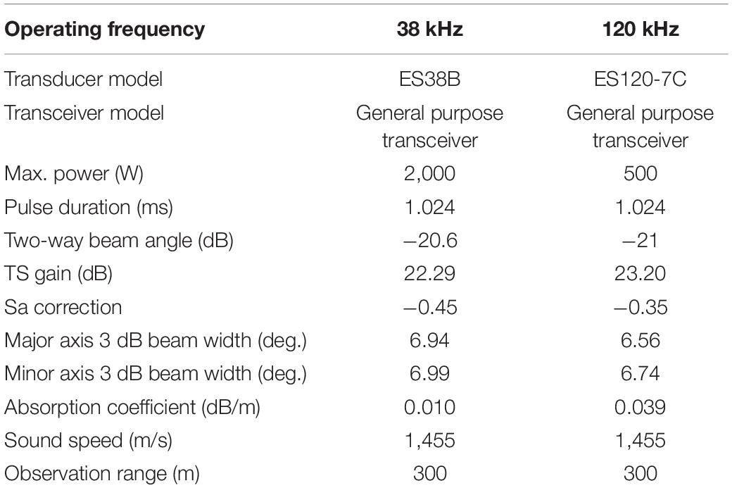
Table 1. The parameters of transceiver calibrated for the acoustic surveys.

FIGURE 1

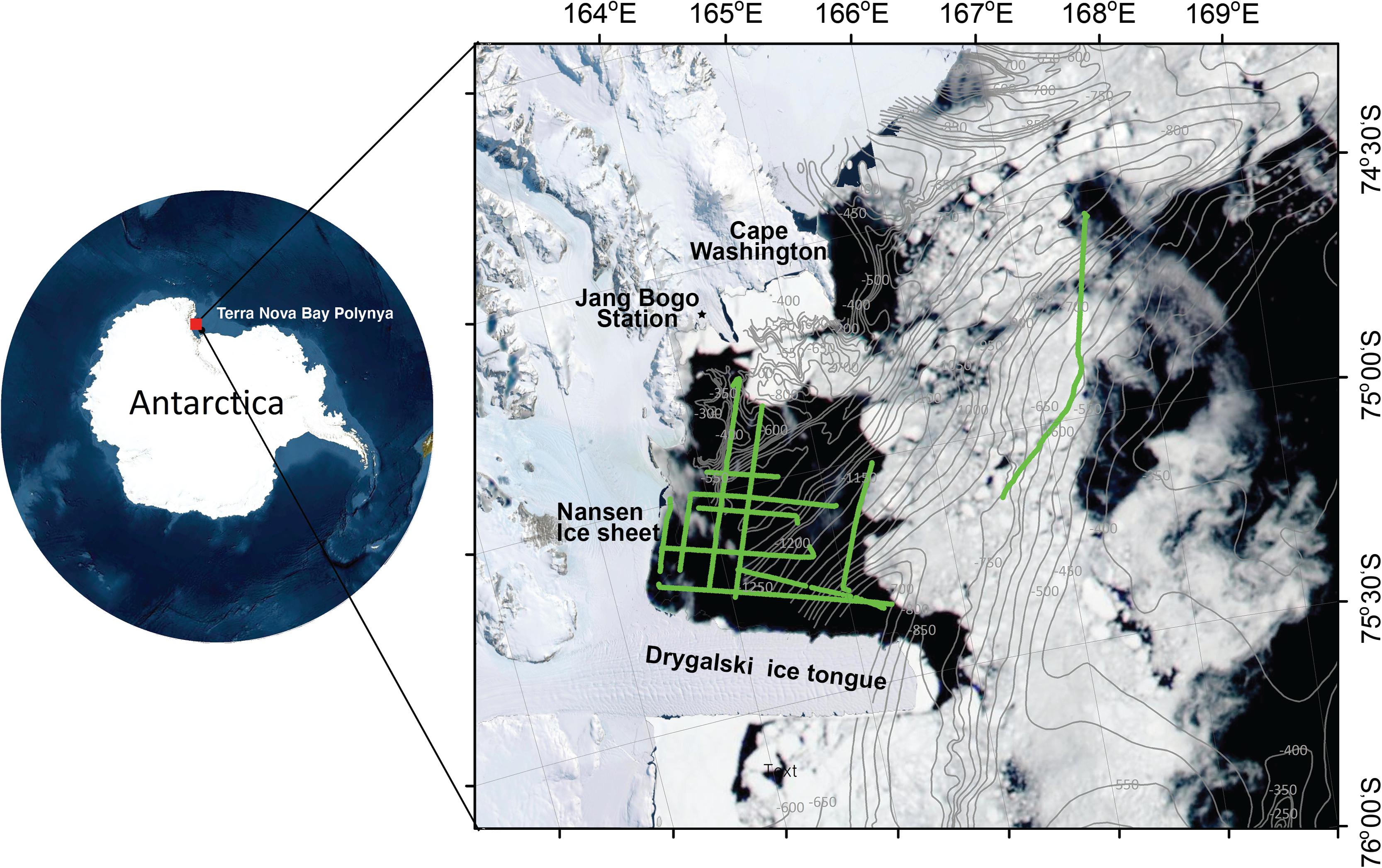
Figure 1. The study area off the Terra Nova Bay polynya, Ross Sea, Antarctica, conducted on 7–14 January 2019. The green line indicates the cruise track line. The gray line with numbers is the bathymetric contour (Davey, 2013). Sea ice distribution, which was from Moderate Resolution Imaging Spectroradiometer (MODIS) on NASA’s Aqua satellite on January 4, 2019, is overlapped.

Acoustic Data Analysis

The raw acoustic data at 38 and 120 kHz from the echosounder were analyzed using Echoview (ver. 10, Echoview Software Pty. Ltd.). The calibration parameters were applied in the raw data. This study was carried out on the icebreaker RV Araon with an EK60 sounder (38 and 120 kHz), an EM122 multibeam echosounder (12 kHz), and an acoustic Doppler current profiler (ADCP; 38 kHz) installed and operating at the same time. Due to the instability of the synchronization unit of these acoustic instruments, substantial interference noise occurred at 38 kHz in the EK60. In case of background noise, it was frequency dependent, and a higher level of background noise was observed in the 120 kHz data than in the other data. First, to remove the surface noise generated by ice and rough seas, data above 4 m were excluded from further analysis. The signal-to-noise ratio (SNR) was improved by applying several noise removal algorithms. The noise removal methods treated the volume backscattering strength (Sv, dB re 1 m²/m³) echogram as an array of values, and individual data points were identified by the vertical sample number and ping number. Second, background noise was estimated and eliminated by applying a background noise removal algorithm. This algorithm provides potentially accurate estimates of the background noise for each ping and subtracts it from each sample (De Robertis and Higginbottom, 2007; Echoview, 2020). Third, the impulse noise removal and transient noise removal algorithms introduced by Ryan et al. (2015) were used to eliminate the noise generated by wave-hull collisions and instrument interference. The combination of operators identified and adjusted the scattering values that are higher than other surrounding pings at the same depth (Perrot et al., 2018; Echoview, 2020). Some other noise spikes and missing pings often appeared on echograms and were manually defined as “bad data.” Lastly, visual scrutinization was used to ensure that krill-like echoes remained for the analysis and noises were excluded. In addition, echograms at different frequencies were examined at a common observation range, which was determined by the SNR as a function of the target parameters, echosounder parameters, acoustic propagation, and noise (Kang et al., 2002). In this study, the observation range was applied to a depth of 300 m.

Krill species identification was performed using the difference of the MVBS, also known as the dB difference method. The dB difference method relies on the frequency characteristics of sound scattering by marine organisms. Fluid-like zooplankton such as krill are characterized by fluctuations between low frequencies e.g., 38 kHz (the Rayleigh scattering region), and high frequencies, e.g., 120 kHz (the geometric scattering region; Kang et al., 2002; Korneliussen and Ona, 2003). Thus, the sound scattering difference between 38 and 120 kHz is large, providing a good method for species classification. The noise-filtered data of the 38 and 120 kHz echograms were resampled to a depth of 2 m using 300 m horizontal distance bins. The MVBS_120–38 dB window was used to identify krill echoes. Previous studies have applied wide MVBS_120–38 ranges for krill, i.e., 2–12 dB (Watkins and Brierley, 2002; Fielding et al., 2014), 2–16 dB (Demer, 2004; Jarvis et al., 2010; Krafft et al., 2015), 4–16 dB (Reiss et al., 2008), and 4.9–12 dB (Choi et al., 2018). The most commonly used MVBS_120–38 range (2–16 dB) was applied in this study because no biological sampling was performed. The krill echoes were selected using the data range bitmap algorithm, and the signals that were not selected as krill were masked out. The portions of the 120 kHz Sv echogram attributed to krill were integrated into a cell (300 m in the horizontal direction and 10 m in the vertical direction) until the entire observation range to examine the vertical distributions of krill. The nautical area scattering coefficient (NASC, m²/nm²) known as S_A is calculated as the integral of the Sv values from 10 to 300 m for the horizontal distributions of krill:

$$\text{NASC}=\underset{\text{z}2}{\overset{\text{z}1}{\int }}{s}_v\mathrm{dz}4\mathrm{\pi }{\mathrm{\hspace{0.33em}\hspace{0.33em}1852}}^2(1)$$

where z1 and z2 are given water depths. The NASC is calculated for a given cell or region of height T as

$$\text{NASC}={\mathrm{\hspace{0.33em}10}}^{\text{Sv}\mathrm{\_}\text{mean}/10}\times \mathrm{T}\times 4\mathrm{\pi }\times {1852}^2(2)$$

Spatial Distribution of Krill

The spatial distribution in the marine structure, including the krill distribution, is often described over a wide area (Guidetti et al., 2014) and is poorly understood at short-term seasonal time scales and local spatial scales (Mustamäki et al., 2015). This study examined a small region of the TNBP (<2,000 km²). The spatiotemporal distribution of krill aggregations and the associated environmental conditions were determined by comparing areas with low and high NASC values. Nast et al. (1988) reported that the separation of low- and high-value areas was related to the actual krill biomass varying from 10 to 50 g/1,000 m³ near Elephant Island in the Antarctic Peninsula. A number of studies have estimated the biomass and density of krill in the Ross Sea. The details are explained in section “Discussion.” Various values of the krill biomass and density in different units have been reported. It was nearly impossible to apply one value to determine low and high areas of the krill population because this study utilized the acoustic scattering strength (i.e., the NASC values). To show the Antarctic krill density in the Scotia Sea in different seasons such as spring 2006, summer 2008, and autumn 2009, Fielding et al. (2012) applied the 75th percentile of their densities. A low density of Antarctic krill off East Antarctica was widely distributed in the austral summer of 2006 and was defined to be lower than the 75th percentile of krill density (Jarvis et al., 2010). Accordingly, the study area was divided into low- and high-value areas on the basis of the third NASC quartile in this study. The areas with NASC values less than the third quartile were categorized as low-value areas, and the areas with NASC values greater than the third quartile were categorized as high-value areas.

Interpolation of Environmental Parameters

Marine environmental information, such as the water temperature, salinity, and chlorophyll, was analyzed using Ocean Data View (ODV, ver. 5.2.1, AWI). The data interpolating variational analysis (DIVA) gridding algorithm was implemented to analyze and spatially interpolate the environmental data in an optimal way by taking the coastlines and bathymetry features into account (Florou et al., 2014). This method is comparable to the optimal interpolation (OI) method, which is widely used to interpolate weather data and allows computation of the relative error variance of the analyzed field (Tandaeo et al., 2011). The DIVA gridding algorithm creates a finite element grid that provides high-resolution spatial variable values and a good representation of coastlines (Troupin et al., 2012). The variational inverse method was applied to estimate surrounding data points based on the distances between each point and their error values. The background fields at each data point were then subtracted from each data value and multiplied by the alpha weight and added together (Tandaeo et al., 2011). This gridding method was chosen because it is more computationally advanced and provides several more advantages than the other ODV weighted averaging methods (Jena et al., 2013). Additionally, the interpolated environmental data were extracted on the basis of the locations of the cruise track lines for statistical analysis with the acoustic data using ArcMap (ver. 10.2, Esri).

Statistical Analysis

Statistical analysis was performed to determine whether significant differences existed between low-value areas and high-value areas and to examine the relationship between the acoustic and environmental data. A non-parametric test (Mann–Whitney U test) was performed to examine the difference between the low-value and high-value areas. The dependent variables included in the analysis were temperature, salinity, and chlorophyll. Spearman’s rank order correlation was calculated between the NASC of krill and the environmental parameters (temperature, salinity, and chlorophyll) extracted from the location of the cruise track lines to verify the significance of the relationships. Thus, the geographic locations of the NASC and the environmental parameters were equal. The statistical analyses were performed in SPSS (ver. 25, IBM).

Results

The echograms, which were processed with various noise removal algorithms and krill identification techniques, indicated the presence of acoustic scattering layers composed of krill. The original Sv echogram and the krill identified echogram at 120 kHz on 07 January are shown in Figure 2 as examples. Horizontal layers appeared continuously throughout the cruise track lines below 4 m to a depth of 150 m in the water column (Figure 2B). The krill aggregations were evidently distributed in the epipelagic zone, mainly appearing at 50–100 m (Figures 2B,E). An expanded original Sv echogram showed vertically sharp noises and krill signals around 200 m (Figure 2C), and the same echogram displayed only krill signals when various noise removal algorithms were applied (Figure 2D). Another example of a noise-removed echogram shows dense krill signals around 50 m (Figure 2D). Note that the zoomed-out echograms (Figures 2A,B) do not present detailed echo signals.

FIGURE 2

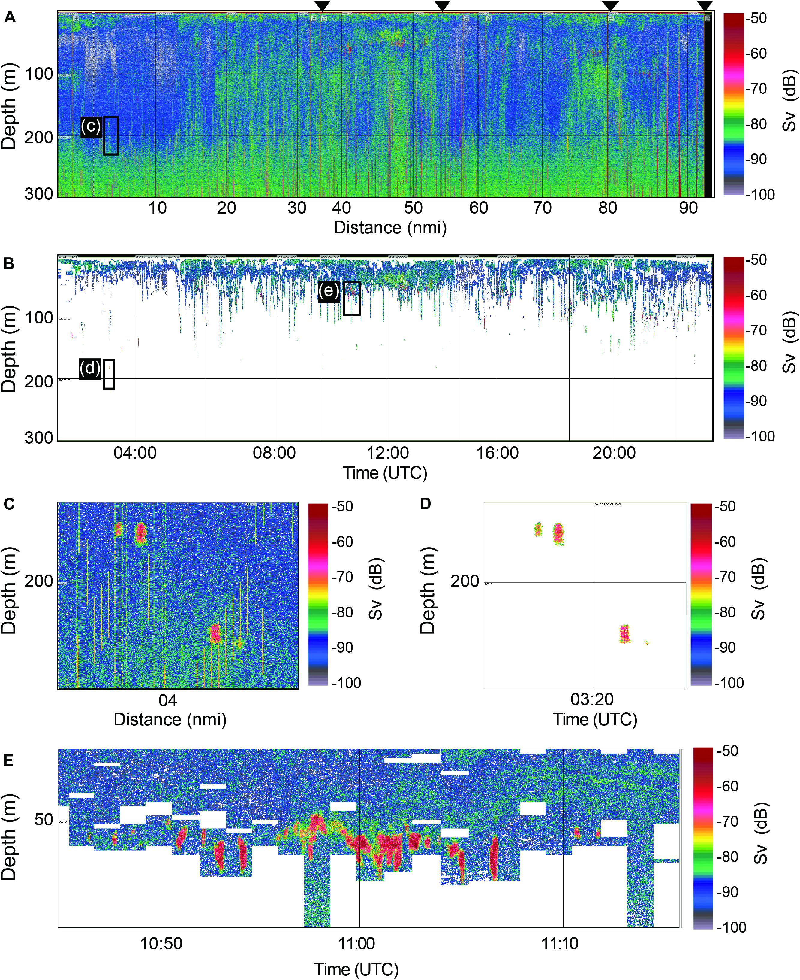
Figure 2. Example echograms. The original Sv echogram at 120 kHz on 7 January 2019 (A), the corresponding noise cleaned echogram (B), the expanded echogram from the black box in the Sv echogram around 200 m (C), the expanded echogram from the box in black in the noise cleaned echogram around 200 m (D), the expanded echogram from the black box in the noise cleaned echogram around 50 m (E). Black triangles indicate the cruise track line, which means that there were four cruise track lines on that day.

The vertical distribution of krill across the TNBP was described from the surface to 300 m, with intervals of 10 m (Figure 3). In regards to depth, the sum of the NASC values between 10 and 30 m accounted for 25.8 m²/nm² (31.7%), which was the highest proportion among the depth layers. The second NASC peak was between 270 and 300 m, with a value of 24.2 m²/nm² (29.8%), and the third peak was from 70 to 110 m with 18.9 m²/nm² (23.2%). The vertical NASC profile indicated that, overall, krill tended to dwell mostly up to 110 m, with some dwelling at depths of 270–300 m.

FIGURE 3

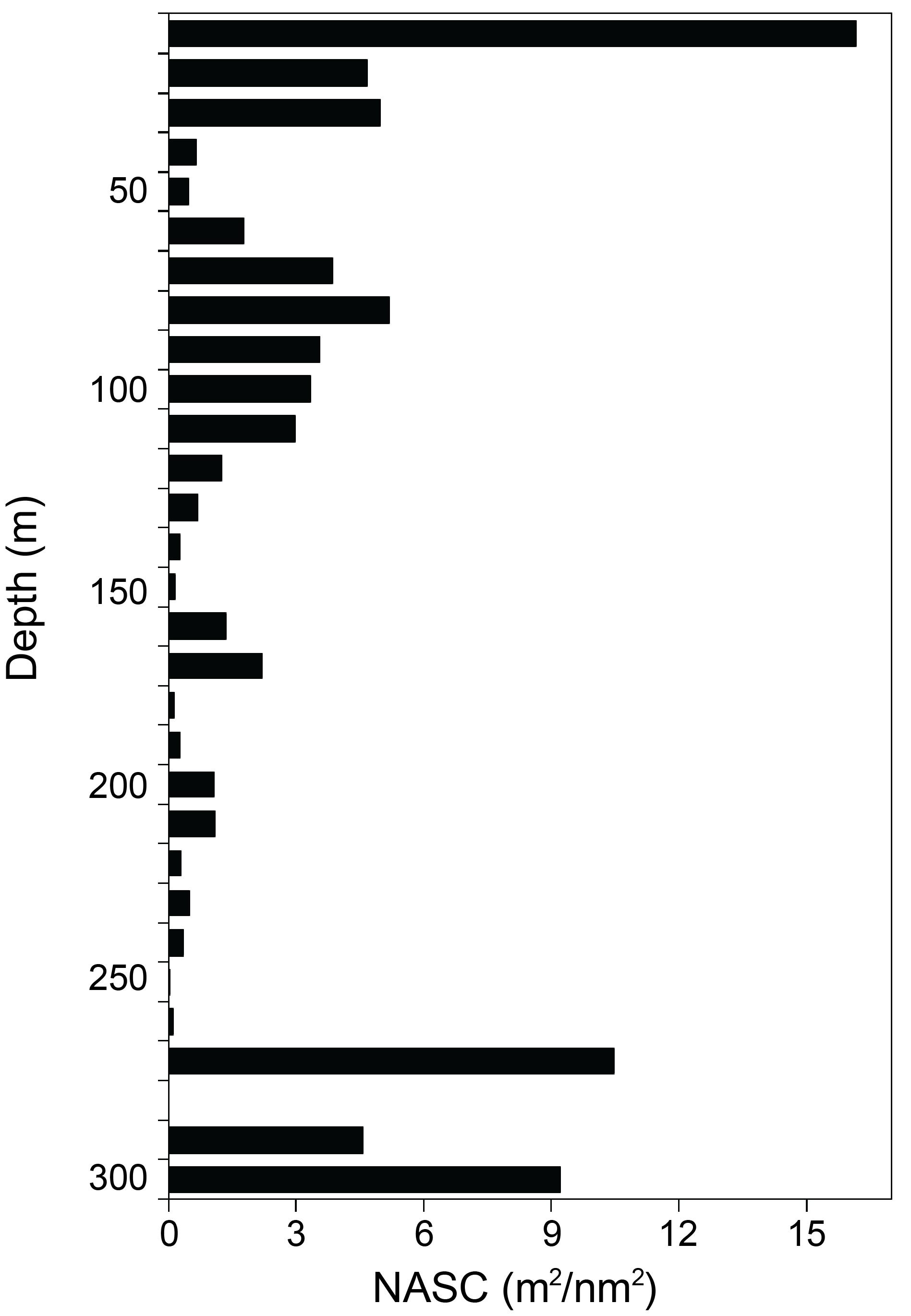
Figure 3. The vertical distribution of krill NASC values, averaging every 10 m using the exported NASC in 300 m in horizontal and 10 m in vertical on 7–14 January 2019.

The horizontal distribution of krill is exhibited in Figure 4. The NASC values were categorized to determine the low-value and high-value areas based on the third quartile values (19.4 m²/nm²). The smallest circle in black indicates the low-value areas. The highest NASC value (3,237.6 m²/nm²) occurred in the Drygalski Ice Tongue (75°12′S and 165°20′E). The cruise track line that was far from the other lines had a very low NASC value. The orange circles showing relatively high NASC values are located close to the coast, except for one (approximately 75°10′S and 165°E).

FIGURE 4

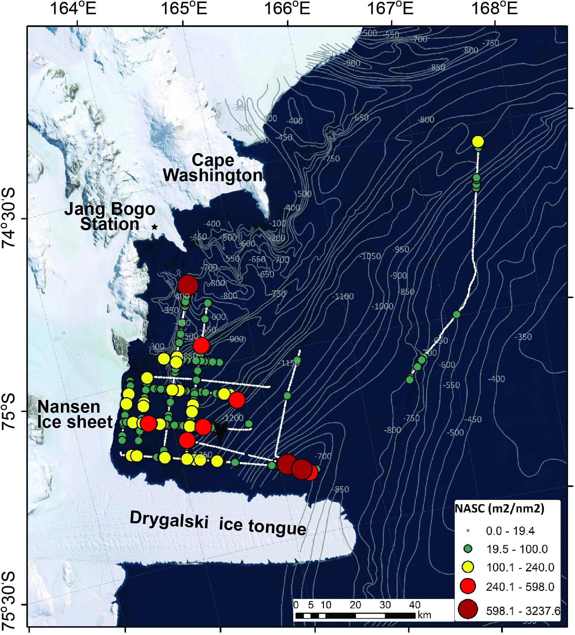
Figure 4. The horizontal distribution of krill NASC values, which were integral of Sv values from 10 m to 300 m, on 7–14 January 2019.

The interpolated environmental parameters along with the NASC values are presented in Figure 5. In the study area, the water temperature was relatively evenly distributed compared to the other two parameters. The salinity seemed to be relatively low along the coastline. The chlorophyll had roughly two different sections based on a longitude of approximately 165°E. During the survey time, the water temperature, which was selected in accordance with the locations of the cruise track lines, varied between 0.3 and 2.0°C [mean = 0.9, standard deviation (SD) = 0.4], the salinity ranged from 32.6 to 34.1 psu (mean = 33.1, SD = 0.4), and the chlorophyll ranged from 0.9 to 4.9 mg/m³ (mean = 3.4, SD = 1.1). Based on the spatial distribution with the interpolated environmental parameters, the low-value areas had relatively high temperatures, high salinities, and low chlorophyll, although the difference in the environmental parameters between the low-value and high-value areas was minor. The high-value areas had temperatures of 0.3–2.0°C (mean = 0.8, SD = 0.4), salinities of 32.6–33.9 psu (mean = 33.0, SD = 0.3), and chlorophylls of 0.9–4.9 mg/m³ (mean = 3.7, SD = 0.4). Meanwhile, the low-value areas had water temperatures ranging from 0.3 to 2.0°C (mean = 1.0, SD = 0.4), salinities of 32.6–34.1 psu (mean = 33.1, SD = 0.4), and chlorophylls of 0.9–4.9 mg/m³ (mean = 3.3, SD = 1.1). It was concluded that the water temperature was significantly higher in the low-value area than in the high-value area (U = 61,602.5, p < 0.01). The salinity was higher in the low-value area than in the high-value area, although the difference was not significant (U = 83,516.5, p = 0.602). The chlorophyll was significantly higher in the high-value area than in the low-value area (U = 64,109.5, p < 0.01).

FIGURE 5

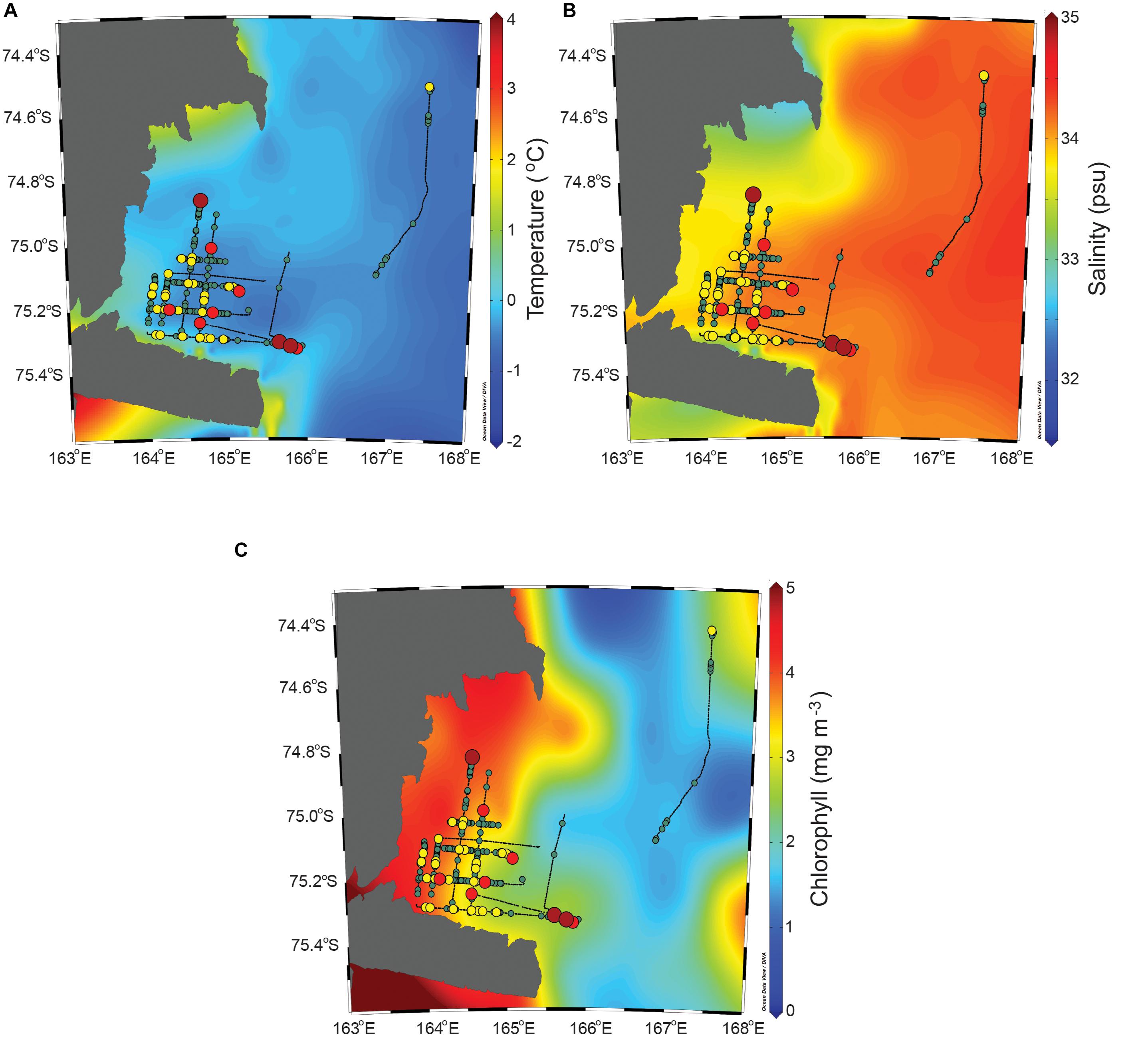
Figure 5. The interpolated water temperature, salinity, and chlorophyll along with the horizontal distribution of the krill NASC values. The legend of NASC is the same as that in Figure 4.

The Spearman’s rank order correlation was calculated between the NASC values and the environmental parameters. The relationship between the NASC values of the low-value areas and the environmental parameters extracted from the locations of the low-value areas and the relationship between the NASC values of the high-value areas and the environmental parameters extracted from the locations of the high-value areas were assessed. In the low-value areas, there was a weak negative correlation between the NASC value and the temperature (r_s = −0.227, n = 718, p < 0.01) and a very weak negative correlation between the NASC value and the salinity (r_s = −0.090, n = 718, p = 0.016). However, there was a very weak positive correlation between the NASC value and the chlorophyll content (r_s = 0.094, n = 717, p = 0.012). In the high-value areas, there was a very weak negative correlation between the NASC value and the salinity (r_s = −0.187, n = 238, p = 0.004), and there were no statistically significant correlations between the NASC value and the temperature (r_s = −0.107, n = 238, p = 0.098) and between the NASC value and the chlorophyll (r_s = 0.011, n = 238, p = 0.866).

Discussion

Utilization of Noise Removal Methods

Large-scale scientific research in the Southern Ocean has the potential to provide qualitative and quantitative information on the distribution of krill and other pelagic species. However, impediments such as a high level of noise restrict data utility and are typically due to the configuration of the various electric instruments aboard ships (Wang et al., 2016). Additionally, for echosounders, the transmitted sound backscattered to the transducer face includes both echo signals from the targets in the water column and noise, i.e., backscatter from unwanted targets (Kieser et al., 2005). Postprocessing methods have been utilized to filter out noise, including a 7 × 7 convolution filter for investigating krill swarms (Klevjer et al., 2010) and a two-sided comparison filter for handling the acoustic data collected from fishing vessels and research vessels (Anderson et al., 2005; Ryan et al., 2015). However, those methods were designed to evaluate low interference noise levels; therefore, the residual error might remain significant in poor-quality data, with a high level of interference noise. This study applied noise removal algorithms in Echoview (background noise removal, impulse noise removal, and transient noise removal) to eliminate the significant influence of noise. Optimal threshold selection and other settings should be applied to exclude the noise from target signals in consideration of the data quality. A high threshold is applicable for strong acoustic scatters with a high SNR; however, in the case of a lower SNR and weak deeply distributed scatters, a substantial portion may be deleted if a high threshold is applied, especially in low-density aggregations (De Robertis and Higginbottom, 2007). In this study, noise signals outside the threshold were identified and replaced by the mean value of adjacent pings. The final result shows that the background noise outside the krill aggregations was effectively removed, the interference noise was reduced, and the echograms of both frequencies were clearly improved. The threshold was visually determined by identifying a satisfactory discrimination between noise and krill echoes; inevitably, it is possible that some krill echoes overlapped with the noise and were, in turn, mistaken as noise and deleted. In fact, a large amount of time was consumed by scrutinizing the quality of the data in the final stage of data analysis.

Acoustic Method and MVBS_120–38 Window

Using the acoustic method has numerous advantages. For instance, a wide area can be covered in a relatively short time, and information on the distribution and abundance of aquatic organisms is attainable throughout the water column (Simmonds and MacLennan, 2005). Acoustic hardware produces high resolution data, and software can deal with vast volumes of data quickly and accurately. In this context, the CCAMLR adopted this method to monitor marine resources in the Southern Ocean (Hewitt et al., 2004), and the method has become a standard tool for targeting krill. Traditionally, echosounders operate within a frequency range of several dozen to several hundred kHz. The most common frequencies are 38 and 120 kHz, which can be called the de facto “standard” frequencies because 38 kHz represents a low frequency and 120 kHz represents a high frequency, with relatively large detection ranges. Numerous studies have adapted these two frequencies to identify krill species. In particular, the collaborative CCAMLR 2000 project used 38 and 120 kHz to identify krill species and assess the biomass of Antarctic krill across the Scotia Sea (Hewitt et al., 2004; Watkins et al., 2004). Therefore, 38 and 120 kHz were appropriate frequencies for identifying the krill species in this study.

One issue considered in this study was the range of the MVBS difference for krill identification. Previous studies in the Scotia Sea have shown that krill species can be visually identified by 120 kHz echograms via the MVBS difference technique at 38 and 120 kHz (Watkins and Brierley, 2002). In addition, a theoretical approach based on the target strength model confirmed that the range of 2–16 dB likely accounts for large assemblages of 10-60 mm krill (CCAMLR, 2005). In this study, the MVBS_120–38 range from 2 to 16 dB was considered based on the fact that a great number of Antarctic krill and ice krill inhabit the Ross Sea in the austral summer (Azzali and Kalinowski, 2000; Azzali et al., 2006; Guglielmo et al., 2009; Murase et al., 2013). Madureira et al. (1993) determined the MVBS differences that can be used to differentiate Antarctic krill (2–12 dB) from other Southern Ocean zooplankton species. Some studies have successfully distinguished ice krill using MVBS_120–38 ranges of >13.8 dB (Azzali et al., 2004) and 12.4–17.9 dB (La et al., 2016). Moreover, Chu and Wiebe (2005) found that the acoustic properties of ice krill were lower than those of Antarctic krill with similar body lengths. MVBS differences, namely the frequency response, are a function of the size, orientation, and physical properties of the target (Figure 1 of Korneliussen and Ona, 2003). The histogram of the range of the MVBS differences at 38 and 120 kHz in this study is moderately even, although it is not shown. Without consideration of the swimming orientation, small and large krill seemed to be evenly distributed in this study.

Distribution and Density of Krill in the Ross Sea

To date, a number of studies have reported the density or biomass of Antarctic krill and ice krill in the Ross Sea as well as their spatial distribution. The temporal results can be summarized as follows. From 4 January to 4 February 1988 and on 21 February 1988 in the Ross Sea, the mean numbers of adult, juvenile, and larval ice krill were assessed to be 20, 87, and, 14,764 ind/m², respectively. The high larval concentration occurred in the shelf region of Terra Nova Bay (74°45′S and 165°E), which is very similar to our study area (Guglielmo et al., 2009). In the early summer of 1989 and 1990, under the condition of ice-free waters, and in the late spring of 1994, under partial ice cover, the mean density of Antarctic krill was estimated to be approximately 33 t/nm² and 100–250 t/nm², respectively. In light of the spatial distribution, in the beginning of summer, a high level of Antarctic krill biomass occurred on the continental slope (between 71 and 73°S), and in the late spring, the krill were concentrated over the continental shelf (between 73 and 75°S). Meanwhile, ice krill were found to the southward (from 75°S up to the Ross Sea Ice Barrier) and west (from 75°S to 171°E toward Terra Nova Bay). As an example of net sampling, 79,881 ice krill individuals were caught at 74°45′S and 171°13′E on 14 December 1994 (Azzali and Kalinowski, 2000). In November 1994, December 1994, December 1997, and January 2000, the estimated mean density of ice krill was 1.8, 1.6, 1.4, and 0.7 t/km², respectively, and the biomass was 0.19, 0.21, 0.19, and 0.14 million tonnes, respectively. For Antarctic krill, the mean density was 21.9, 21.4, 16.3, and 11 t/km², respectively, the biomass was 2.3, 2.7, 2.2, and 1.2 million tonnes, respectively (Azzali et al., 2006). Two krill species occupied clearly separate regions. Most Antarctic krill were found on the border between the Ross Sea and the Southern Ocean, whereas ice krill dominated in the coastal area south of Coulman Island (between 73° and 74°S). From 9 January to 6 February 2000, ice krill were widely distributed in the Ross Sea and were mainly concentrated southward from 74°S, with a mean density of 19.1 ind./1,000 m³ (3.0 g/1,000 m³); Antarctic krill were mainly found from the area north of the continental shelf to the continental slope (71–73°S), with a mean density of 10.9 ind./1,000 m³ (9.3 g/1,000 m³; Sala et al., 2002). The study area in the above publications included this study area. From 26 December 2004 to 6 February 2005 in the Ross Sea under nearly completely ice-free conditions, ice krill were exclusively dominant on the continental shelf and abundant in the eastern basin area (72–80°S and 170°E–170°W); Antarctic krill were found in Terra Nova Bay (70–72°S, 170°E). The maximum densities (biomass) of ice krill and Antarctic krill were approximately 56 and 13 ind./m² (4 and 6 g/m²), respectively (Taki et al., 2008). In addition, thysanoessa spp. was widely distributed north of the continental slope in the waters adjacent to the Ross Sea (60–70°S and 170°E–180°). In a relatively wide area of the Ross Sea (170°E–160°W and 70–78°S) from 14 January to 15 February 2005, ice krill were found in the southwestern part of the study area, whereas Antarctic krill were found in the northeastern part. Their maximum densities were 13 and 57 g/m², respectively. Two krill species seemed to be diagonally separated in that area (Murase et al., 2013). On 23–25 January 2014, dense swarms of ice krill were found in the central coastal area of the western Ross Sea. The mean density of ice krill in 2014 was 72.4 t/nm². In particular, ice krill were found south of Coulman Island (73.5°S) off Terra Nova Bay and the Drygalski Ice Tongue (near 75°S), where the highest density of krill was found in this study. Antarctic krill were concentrated on the northern border of the Ross Sea (71.5–72.5°S and 172–175.5°E), with a mean density of 158.9 t/nm² (Leonori et al., 2017). Accordingly, the northern and northwestern areas of the Ross Sea seemed to be favorable for Antarctic krill, and the southern and southwestern areas seemed to be favorable for ice krill in January. The krill biomass varied based on the season and year. Scientific surveys have focused on the austral spring and summer (nearly ice-free times) due to the navigational constraints of ship-based measurements during other seasons. In this study, the acoustic krill identification was not verified using methods such as net sampling. However, a number of the aforementioned studies, in particular the studies performed by Italian scientists, support the existence of krill in the Ross Sea in January. The study areas are in and near Terra Nova Bay (74.4–75.4°S and 163–168°E). It can be assumed that the majority of the detected krill were ice krill, with some detected Antarctic kill, although this did not mean that krill were the only species observed in this study.

Vertical Distribution of Krill

Several studies on the vertical distribution pattern of krill around Antarctica have been reported. Near Deception Island in the Antarctic Peninsula, ice krill were diversely distributed in the depth layer of 10–120 m throughout the day based on eleven net hauls during a single 24-h period (Everson, 1987). On the west coast of the Antarctic Peninsula, ice krill occurred in the depth layer of 50–290 m during the winter, without a peak in the depth distribution (Nordhausen, 1994). In the Weddell Sea, a high Antarctic krill density was observed under ice between 1 and 13 km south of the ice edge using an autonomous underwater vehicle (AUV) in 63°S (Brierley et al., 2002). In the Ross Sea in the austral summer of 1987–1988, ice krill larvae were found mainly in the 0–50 m depth layer within 0–100 m, with a sharp decreasing trend down to 250 m, and then extremely low values were observed from 600 to 700 m. Juveniles were rather widely distributed, with a declining distribution in the upper 200 m, and 67% of total juveniles occurred in the first 100 m, whereas only 1% was found between 550 and 600 m. Adult were mainly found at 50–100 m (41%), with the distribution decreasing down to 600 m (Guglielmo et al., 2009). In the Ross Sea from 16 January to 7 February 2000, the maximum depth of the net was between 35 and 91 m to sample ice krill, indicating that the main target krill resided in relatively shallow water layers (Sala et al., 2002). In addition, in the Ross Sea from 26 December 2004 to 6 February 2005, adult and juvenile ice krill were found at 200–300 m in the colder water of the continental shelf from stratified tows at depths of up to 1,000 m. Overall, the peak biomass of ice krill occurred in the middle depth layers (100–400 m), and adult Antarctic krill were mainly found between 400 and 600 m (Taki et al., 2008). In the Scotia Sea in January–February 2000, most acoustically detected krill were found from 6 to 100 m, with a peak of 40 m that decreased sharply until 200 m (Kasatkina et al., 2004). In the Scotia Sea, the mean depth of Antarctic krill swarms was distributed in 100 m in spring 2006, 160 m in summer 2008, 150 m in autumn 2009. The 25–75th percentile of krill swarm depths was 20–100 m, 40–60 m, and 50–300 m, respectively (Fielding et al., 2012). In the East Antarctica (30–80°E), the majority of Antarctic krill were detected in the top 100 m of the water column, centered around 50 m, and there was a lack of evidence for krill below 250 m (Jarvis et al., 2010). In the Amundsen Sea coastal polynya, the major distributed depth of ice krill was from 20 to 250 m, with a nearly constant horizontal layer. The weighted mean depth of ice krill was 50–150 m (La et al., 2015b). In the north Lützow-Holm Bay (64–70°S and 34–43°E) in the Cosmonaut Sea, based on midwater tows in six different water layers between the surface and 2,000 m, Antarctic krill occurred mainly in the 0–50 m layer, followed by the 100–200 m layer; ice krill were very scarce in the 0–100 m and 200–500 m layers in January 2005, and Antarctic krill were abundant in the 0–50 m layer (Ono and Moteki, 2017). Accordingly, krill are diversely distributed from the surface to 600 m in various areas around Antarctica. However, one of the major distribution depths of krill seems to be in rather shallower water such as 100 m. In particular, juveniles seemed to prefer the upper layer, while adults occur in rather deeper layers of the water column in the Ross Sea (Taki et al., 2008; Guglielmo et al., 2009). The three peaks in the 10–30, 70–110, and 270–300 m layers from this study have been observed in previous studies conducted in the Ross Sea. In fact, a different methodology for obtaining information on the vertical distribution of krill might have yielded different results. Some fishing gear reaches depths of up to 1,000 m, and other equipment is targeted for shallow waters, for example, depths of 200 m. AUVs have obvious short detection ranges, although they have great mobility and accessibility. For the acoustic method, the detection range is limited by frequency. Therefore, it was difficult to acquire information on the vertical distribution of krill deeper than 300 m in this study.

Krill in Relation to Environmental Attributes

In the austral summer in the Ross Sea, the polynya (ice-free areas) become larger, resulting in a considerably wide canal between the Ross Sea and the South Ocean. In particular, when the ice edge retreats in early January in the Ross Sea, the spatial extent of the Antarctic krill extends beyond the Ross Sea, and some portion of them spread into the ocean waters, whereas the ice krill seem to be delimited to the Ross Sea (Azzali et al., 2006; Guglielmo et al., 2009; Leonori et al., 2017).

From November to January, as the polynya ice front progresses northward, the length of the ice edge along Terra Nova Bay and the Ross Sea increases as the amount of ice-free water exposed to sunlight increases. As a result of ice melting, the condition of the upper layers in the water column may affect the formation of phytoplankton and zooplankton blooms and the release of algae, which are the major food for krill (Hecq et al., 2000; Fonda Umani et al., 2005). Due to ice melting, low salinities appear to be connected with a high density of Antarctic krill (Murase et al., 2013) because high productivity levels provide a favorable environment for krill, and ice edges can play a role as refuges in early stages of development (Brierley et al., 2002; Nicol, 2006). In this study, the spatial distribution of krill seemed to be influenced by the polynya environment; in particular, the low salinity around the high-value areas seemed to be related to this aspect. Krill appear to be sensitive to salinity changes. In general, the increase in salinity close to the Ross Sea potentially induces modifications in krill recruitment and affects the decrease in krill abundance (Brierley et al., 2002; Nicol, 2006; Rusciano et al., 2013); inevitably, this might have influenced the variability of the NASC values in this study.

In the late austral summer in the Ross Sea, Antarctic krill showed no relationship with the water temperature, but ice krill were marginally more abundant under higher temperatures. The density of Antarctic krill and ice krill was inversely correlated with salinity. High densities of Antarctic krill were found regardless of the level of fluorescence, whereas the ice krill biomass was positively correlated with fluorescence, which was related to trophic factors (Leonori et al., 2017). The dietary pattern of ice krill changes from carnivorous to omnivorous at the beginning of the spring phytoplankton bloom (Pakhomov et al., 1998). Therefore, it is plausible for ice krill to be concentrated where primary production is high. For this reason, high-value areas had high chlorophyll in this study. Additionally, at the circumpolar scale, a high krill distribution can be observed in regions with moderate chlorophyll concentrations (Atkinson et al., 2008) and relatively warm temperatures (Nicol, 2006). In this study, relatively warm temperatures (0.9 ± 0.4°C) were observed, similar to a previous study that documented warm surface water (0.3–1.5°C) in coastal areas in Terra Nova Bay during the austral summer (Guglielmo et al., 2009). Long-term studies in the Southern Ocean have suggested that changes in the marine environment have contributed to the variability in the krill distribution (Fielding et al., 2014). However, the relationship between krill biomass and local environmental properties is highly variable (Santora et al., 2012; Siegel et al., 2013).

Data Availability Statement

All datasets used in this study are available upon request from the first author (mk@gnu.ac.kr) or the corresponding author (hsla@kopri.re.kr).

Author Contributions

HL conceived of the study. WS collected the acoustic data. MK and RF analyzed the acoustic and physical data. MK, RF, WS, HL, and J-HK contributed to the study design and data discussion. MK, RF, and HL wrote the manuscript. All authors contributed to the revision of the work.

Funding

This research was supported by the “Ecosystem Structure and Function of Marine Protected Area (MPA) in Antarctica” project (PM20060), funded by the Ministry of Oceans and Fisheries (20170336), Korea, and the National Research Foundation of Korea (NRF) grant funded by the Korea Government (MSIT) (No. NRF-2018R1A2B6005666). Additional data processing and analysis was supported by the Korea Polar Research Institute grant (PE20140).

Conflict of Interest

The authors declare that the research was conducted in the absence of any commercial or financial relationships that could be construed as a potential conflict of interest.

Acknowledgments

We acknowledge the support and dedication of the captain and crew of IBRV ARAON for completing the field work with positive energy. We thank our field teams who worked together under harsh conditions during the survey. We thank the referees for their valuable and insightful comments and suggestions, which improved this paper in many aspects.

References

Ainley, D. G. (2010). A history of the exploitation of the Ross Sea, Antarctica. Polar Rec. 46, 233–243. doi: 10.1017/S003224740999009X

CrossRef Full Text | Google Scholar

Ainley, D. G., Ballard, G., and Dugger, K. M. (2006). Competition among penguins and cetaceans reveals trophic cascades in the western Ross Sea, Antarctica. Ecology 87, 2080–2093.

Google Scholar

Anderson, C. I. H., Brierley, A. S., and Armstrong, F. (2005). Spatio–temporal variability in the distribution of epi- and meso-pelagic acoustic backscatter in the Irminger Sea, North Atlantic, with implications for predation on Calanus finmarchicus. Mar. Biol. 146, 1177–1188. doi: 10.1007/s00227-004-1510-8

CrossRef Full Text | Google Scholar

Arrigo, K. R., DiTullio, G. R., Dunbar, R. B., Lizotte, M. P., Robinson, D. H., Van Woert, M., et al. (2000). Phytoplankton taxonomic variability and nutrient utilization and primary production in the Ross Sea. J. Geophys. Res. 105, 8827–8846. doi: 10.1029/1998JC000289

CrossRef Full Text | Google Scholar

Arrigo, K. R., and Van Dijken, G. L. (2003). Phytoplankton dynamics within 37 Antarctic coastal polynya systems. J. Geophys. Res. 108:3271. doi: 10.1029/2002JC001739

CrossRef Full Text | Google Scholar

Arrigo, K. R., Van Dijken, G. L., and Bushinsky, S. (2008). Primary production in the Southern Ocean, 1997–2006. J. Geophys. Res. 113:C08004.

Google Scholar

Arrigo, K. R., Worthen, D., Schnell, A., and Lizotte, M. P. (1998). Primary production in Southern Ocean waters. J. Geophys. Res. 103, 15587–15600. doi: 10.1029/2007JC004551

CrossRef Full Text | Google Scholar

Atkinson, A., Nicol, S., Kawaguchi, S., Pakhomov, E. A., Quetin, L. B., Ross, R. M., et al. (2012). Fitting Euphausia superba into Southern Ocean food-web models: a review of data sources and their limitations. CCAMLR Sci. 19, 219–245.

Google Scholar

Atkinson, A., Siegel, V., Pakhomov, E., and Rothery, P. (2004). Long-term decline in krill stock and increase in salps within the Southern Ocean. Nature. 432, 100–103. doi: 10.1038/nature02996

PubMed Abstract | CrossRef Full Text | Google Scholar

Atkinson, A., Siegel, V., Pakhomov, E. A., Rothery, P., Loeb, V., Ross, R. M., et al. (2008). Oceanic circumpolar habitats of Antarctic krill. Mar. Ecol. Prog. Ser. 362, 1–23. doi: 10.3354/meps07498

CrossRef Full Text | Google Scholar

Azzali, M., and Kalinowski, J. (2000). “Spatial and temporal distribution of krill Euphausia superba biomass in the Ross Sea (1989-1990 and 1994),” In Ross Sea Ecology eds F. Faranda, L. Guglielmo, and A. Ianora (Berlin: Springer-Verlag), 434–455.

Google Scholar

Azzali, M., Leonori, I., De Felice, A., and Russo, A. (2006). Spatial-temporal relationships between two euphausiid species in the Ross Sea. Chem. Ecol. 22, S219–S233. doi: 10.1080/02757540600670836

CrossRef Full Text | Google Scholar

Azzali, M., Leonori, I., and Lanciani, G. (2004). A hybrid approach to acoustic classification and length estimation of krill. CCAMLR Sci. 11, 33–58.

Google Scholar

Ballard, G., Jongsomjit, D., Veloz, S. D., and Ainley, D. G. (2011). Coexistence of mesopredators in an intact polar ocean ecosystem: the basis for defining a Ross Sea marine protected area. Biol. Cons. 156, 78–82.

Google Scholar

Belcher, A., Tarling, G. A., Manno, C., Atkinson, A., Ward, P., Skaret, G., et al. (2017). The potential role of Antarctic krill faecal pellets in efficient carbon export at the marginal ice zone of the South Orkney Islands in spring. Polar Biol. 40, 2001–2013. doi: 10.1007/s00300-017-2118-z

PubMed Abstract | CrossRef Full Text | Google Scholar

Bottino, N. R. (1974). The fatty acids of Antarctic phytoplankton and euphausiids, Fatty acid exchange among levels of the Ross Sea. Mar. Biol. 27, 197–204. doi: 10.1007/BF00391944

CrossRef Full Text | Google Scholar

Brierley, A. S., Fernandes, P. G., Brandon, M. A., Armstrong, F., Millard, N. W., McPhail, S. D., et al. (2002). Antarctic krill under sea ice: elevated abundance in a narrow band just south of ice edge. Science 295, 1890–1892. doi: 10.1126/science.1068574

PubMed Abstract | CrossRef Full Text | Google Scholar

Bromwich, D. H., and Kurtz, D. D. (1984). Katabatic wind forcing of the Terra Nova Bay polynya. J. Geophys. Res. 89, 3561–3572. doi: 10.1029/JC089iC03p03561

CrossRef Full Text | Google Scholar

Cavan, E. L., Belcher, A., Atkinson, A., Hill, S. L., Kawaguchi, S., McCormack, S., et al. (2019). The importance of Antarctic krill in biogeochemical cycles. Nat. Commun. 10:4742. doi: 10.1038/s41467-019-12668-7

PubMed Abstract | CrossRef Full Text | Google Scholar

CCAMLR (2005). Report of the Twenty Fourth Meeting of the Scientific Committee. Hobart: CCAMLR.

Google Scholar

Choi, S. G., Yoon, E. A., An, D. H., Chung, S., Lee, J., and Lee, K. (2018). Characterization of frequency and aggregation of the Antarctic Krill using acoustic. Ocean Sci. J. 53, 667–677. doi: 10.1007/s12601-018-0043-x

CrossRef Full Text | Google Scholar

Chu, D., and Wiebe, P. H. (2005). Measurements of sound-speed and density contrasts of zooplankton in Antarctic waters. ICES J. Mar. Sci. 62, 818–831. doi: 10.1016/j.icesjms.2004.12.020

CrossRef Full Text | Google Scholar

Cooper, L. W., Grebmeier, J. M., Larsen, I. L., Egorov, V. G., Theodorakis, C., Kelly, H. P., et al. (2002). Seasonal variation in sedimentation of organic materials in the St. Lawrence Island polynya region, Bering Sea. Mar. Ecol. Prog. Ser. 226, 13–26. doi: 10.3354/meps226013

CrossRef Full Text | Google Scholar

Davey, F. (2013). Contours of Ross Sea Bathymetry (2004). Integrated Earth Data Applications (IEDA). doi: 10.1594/IEDA/100406

CrossRef Full Text | Google Scholar

Davis, L. B., Hofmann, E. E., Klinck, J. M., Piñones, A., and Dinniman, M. S. (2017). Distributions of krill and Antarctic silverfish and correlations with environmental variables in the western Ross Sea, Antarctica. Mar. Ecol. Prog. Ser. 584, 45–65. doi: 10.3354/meps12347

CrossRef Full Text | Google Scholar

De Robertis, A., and Higginbottom, I. (2007). A post-processing technique for estimation of signal-to-noise ratio and removal of echosounder background noise. ICES J. Mar. Sci. 64, 1282–1291. doi: 10.1093/icesjms/fsm112

CrossRef Full Text | Google Scholar

Demer, D. A. (2004). An estimate of error for the CCAMLR 2000 survey estimate of krill biomass. Deep Sea Res. II. 51, 1237–1251. doi: 10.1016/j.dsr2.2004.06.012

CrossRef Full Text | Google Scholar

Echoview (2020). Help File for Echoview. Available at: https://support.echoview.com/ (accessed April 10, 2020).

Google Scholar

Everson, I. (1987). Some aspects of the small scale distribution of Euphausia crystallorophias. Polar Biol. 8, 9–15. doi: 10.1007/BF00297158

CrossRef Full Text | Google Scholar

Fielding, S., Watkins, J. L., Collins, M. A., Enderlein, P., and Venables, H. J. (2012). Acoustic determination of the distribution of fish and krill across the Scotia Sea in spring 2006, summer 2008 and autumn 2009. Deep Sea Res. II. 59–60, 173–188. doi: 10.1016/j.dsr2.2011.08.002

CrossRef Full Text | Google Scholar

Fielding, S., Watkins, J. L., Trathan, P. N., Enderlein, P., Waluda, C. M., Stowasser, G., et al. (2014). Interannual variability in Antarctic krill (Euphausia superba) density at South Georgia, Southern Ocean: 1997–2013. ICES J. Mar. Sci. 71, 2578–2588. doi: 10.1093/icesjms/fsu104

CrossRef Full Text | Google Scholar

Florou, H., Sykioti, O., Evangeliou, N., Mavrokefalou, G., and Tzempelikou, E. (2014). “Remote radiological assessment in the marine environment: SMOS and MODIS observations combined to 137Cs activity concentrations in the Aegean Sea-Greece,” Proceedings of the ICRER 2014 – Third International Conference on Radioecology and Environmental Radioactivity, Barcelona. doi: 10.13140/2.1.2539.9685

CrossRef Full Text | Google Scholar

Fonda Umani, S., Monti, M., Bergamasco, A., Cabrini, M., De Vittor, C., Burba, N., et al. (2005). Plankton community structure and dynamics versus physical structure from Terra Nova Bay to Ross Ice Shelf (Antarctica). J. Mar. Syst. 55, 31–46. doi: 10.1016/j.jmarsys.2004.05.030

CrossRef Full Text | Google Scholar

Foote, K. G., Knudsen, H. P., Vestnes, G., MacLennan, D. N., and Simmonds, E. J. (1987). Calibration of acoustic instruments for fish density estimation: a practical guide. ICES Coop. Res. Rep. 144:69.

Google Scholar

Foote, K. G., and Stanton, T. K. (2000). “Acoustical Methods”, in ICES Zooplankton Methodology Manual, eds R. Harris, P. H. Wiebe, J. Lenz, H. R. Skjoldal, and M. Huntley (Cham: Academic Press) 223–258.

Google Scholar

Gradinger, R. R., and Baumann, M. E. M. (1991). Distribution of phytoplankton communities in relation to the large-scale hydrographical regime in the Fram Strait. Mar. Biol. 111, 311–321. doi: 10.1007/BF01319714

CrossRef Full Text | Google Scholar

Guglielmo, L., Donato, P., Zagami, G., and Granata, A. (2009). Spatio–temporal distribution and abundance of Euphausia crystallorophias in Terra Nova Bay (Ross Sea, Antarctica) during austral summer. Polar Biol. 32, 347–367. doi: 10.1007/s00300-008-0546-5

CrossRef Full Text | Google Scholar

Guidetti, P., Baiata, P., Ballesteros, E., Di Franco, A., Hereu, B., Macpherson, E., et al. (2014). Large-scale assessment of Mediterranean marine protected areas effects on fish assemblages. PLoS One 9:e91841. doi: 10.1371/journal.pone.0091841

PubMed Abstract | CrossRef Full Text | Google Scholar

Hecq, J. H., Guglielmo, L., Goffart, A., Catalano, G., and Goosse, H. (2000). A Modeling Approach to the Ross Sea Plankton Ecosystem: Ross Sea Ecology. Berlin: Springer.

Google Scholar

Hewitt, R. P., Watkins, J., Naganobu, M., Sushin, V., Brierley, A. S., Demer, D. A., et al. (2004). Biomass of Antarctic krill in the Scotia Sea in January/February 2000 and its use in revising an estimate of precautionary yield. Deep Sea Res. 51, 1215–1236. doi: 10.1016/s0967-0645(04)00076-1

CrossRef Full Text | Google Scholar

Hosie, G. W., and Cochran, T. G. (1994). Mesoscale distribution patterns of macro- zooplankton communities in Prydz Bay, Antarctica January to February 1991. Mar. Ecol. Prog. Ser. 106, 21–39. doi: 10.3354/meps106021

CrossRef Full Text | Google Scholar

Jarvis, T., Kelly, N., Kawaguchi, S., van Wijk, E., and Nicol, S. (2010). Acoustic characterization of the broad–scale distribution and abundance of Antarctic krill (Euphausia superba) off East Antarctica (30–80° E) in Jan–March 2006. Deep Sea Res. II. 57, 916–933. doi: 10.1016/j.dsr2.2008.06.013

CrossRef Full Text | Google Scholar

Jena, B., Sahu, S., Avinash, K., and Swain, D. (2013). Observation of oligotrophic gyre variability in the south Indian Ocean: environmental forcing and biological response. Deep Sea Res. I. 80, 1–10. doi: 10.1016/j.dsr.2013.06.002

CrossRef Full Text | Google Scholar

Kang, M., Furusawa, M., and Miyashita, K. (2002). Effective and accurate use of difference in mean volume backscattering strength to identify fish and plankton. ICES J. Mar. Sci. 59, 794–804. doi: 10.1006/jmsc.2002.1229

CrossRef Full Text | Google Scholar

Kasatkina, S. M., Goss, C., Emery, J. H., Takao, Y., Litvinov, F. F., Malyshko, A. P., et al. (2004). A comparison of net and acoustic estimates of krill density in the Scotia Sea during the CCAMLR 2000 Survey. Deep-Sea Res. II. 57, 1289–1300. doi: 10.1016/j.dsr2.2004.06.005

CrossRef Full Text | Google Scholar

Kieser, R., Reynisson, P., and Mulligan, T. J. (2005). Definition of signal-to-noise ratio and its critical role in split-beam measurements. ICES J. Mar. Sci. 62, 123–130. doi: 10.1016/j.icesjms.2004.09.006

CrossRef Full Text | Google Scholar

Klevjer, T. A., Tarling, G. A., and Fielding, S. (2010). Swarm characteristics of Antarctic krill Euphausia superba relative to the proximity of land during summer in the Scotia Sea. Mar. Ecol. Prog. Ser. 409, 157–170. doi: 10.3354/meps08602

CrossRef Full Text | Google Scholar

Korneliussen, R. J., and Ona, E. (2003). Synthetic echograms generated from the relative frequency response. ICES J. Mar. Sci. 60, 636–640. doi: 10.1016/S1054-3139(03)00035-3

CrossRef Full Text | Google Scholar

Krafft, B. A., Skaret, G., Krag, L. A., Rustand, T., and Pedersen, R. (2016). Antarctic krill and ecosystem monitoring survey at South Orkney Islands in 2016. Inst. Mar. Res. Rep. 20, 22.

Google Scholar

Krafft, B. A., Skaret, G., and Knutsen, T. (2015). An Antarctic krill (Euphausia superba) hotspot: population characteristics, abundance and vertical structure explored from a krill fishing vessel. Polar Biol. 38, 1687–1700. doi: 10.1007/s00300-015-1735-7

CrossRef Full Text | Google Scholar

La, H. S., Ha, H. K., Kang, C. Y., Wåhlin, A. K., and Shin, H. C. (2015a). Acoustic backscatter observations with implications for seasonal and vertical migrations of zooplankton and nekton in the Amundsen shelf (Antarctica). Estuar. Coast. Shelf Sci. 152, 124–133. doi: 10.1016/j.ecss.2014.11.020

CrossRef Full Text | Google Scholar

La, H. S., Lee, H., Fielding, S., Kang, D., Ha, H. K., Atkinson, A., et al. (2015b). High density of ice krill (Euphausia crystallorophias) in the Amundsen sea coastal polynya, Antarctica. Deep-Sea Res. I. 95, 75–84. doi: 10.1016/j.dsr.2014.09.002

CrossRef Full Text | Google Scholar

La, H. S., Lee, H., Kang, D., Lee, S. H., and Shin, H. C. (2016). Volume backscattering strength of ice krill (Euphausia crystallorophias) in the Amundsen Sea coastal polynya. Deep-Sea Res. II. 123, 86–91. doi: 10.1016/j.dsr2.2015.05.018

CrossRef Full Text | Google Scholar

La, H. S., Park, K., Wåhlin, A., Arrigo, K. R., Kim, D. S., Yang, E. J., et al. (2019). Zooplankton and micronekton respond to climate fluctuations in the Amundsen Sea polynya, Antarctica. Sci. Rep. 9:110087. doi: 10.1038/s41598-019-46423-1

PubMed Abstract | CrossRef Full Text | Google Scholar

Leonori, I., Andrea, D. F., Canduci, G., Costantini, I., Biagiotti, I., Giuliani, G., et al. (2017). Krill distribution in relation to environmental parameters in mesoscale structures in the Ross Sea. J. Marine Syst. 166, 159–171. doi: 10.1016/j.jmarsys.2016.11.003

CrossRef Full Text | Google Scholar

Li, C. L., Sun, S., Zhang, G. T., and Ji, P. (2001). Summer feeding activities of zooplankton in Prydz Bay, Antarctica. Polar Biol. 24, 892–900. doi: 10.1007/s003000100292

CrossRef Full Text | Google Scholar

Madec, G., Rahier, C., and Chartier, M. (1988). A comparison of two-dimensional elliptic solvers for the streamfunction in a multilevel ogcm. Ocean Model. 78, 1–6.

Google Scholar

Madureira, L. S. P., Ward, P., and Atkinson, A. (1993). Differences in backscattering strength determined at 120 and 38 kHz for three species of Antarctic macroplankton. Mar. Ecol. Prog. Ser. 93, 17–24. doi: 10.3354/meps093017

CrossRef Full Text | Google Scholar

Mangoni, O., Saggiomo, M., Bolinesi, F., Castellano, M., Povero, P., Saggiomo, V., et al. (2019). Phaeocystis antarctica unusual summer bloom in stratified antarctic coastal waters (Terra Nova Bay, Ross Sea). Mar. Environ. Res. 151:104733. doi: 10.1016/j.marenvres.2019.05.012

PubMed Abstract | CrossRef Full Text | Google Scholar

Massom, R. A., Hill, K. L., Lytle, V. I., Worby, A. P., Paget, M. J., and Allison, I. (2001). Effects of regional fast-ice and iceberg distributions on the behaviour of the Mertz Glacier polynya, East Antarctica. Ann. Glaciol. 33, 391–398. doi: 10.3189/172756401781818518

CrossRef Full Text | Google Scholar

Murase, H., Kitakado, T., Hakamada, T., Matsuoka, K., Nishiwaki, S., and Naganobu, M. (2013). Spatial distribution of Antarctic minke whales (Balaenoptera bonaerensis) in relation to spatial distributions of krill inthe Ross Sea, Antarctica. Fish. Oceanogr. 22, 154–173. doi: 10.1111/fog.12011

CrossRef Full Text | Google Scholar

Mustamäki, N., Jokinen, H., Scheinin, M., Bonsdorff, E., and Mattila, J. (2015). Seasonal small-scale variation in distribution among depth zones in a coastal Baltic Sea fish assemblage. ICES J. Mar. Sci. 72, 2374–2384. doi: 10.1093/icesjms/fsv068

CrossRef Full Text | Google Scholar

Nast, F., Kock, K.-H., Sahrhage, D., Stein, M., and Tiedtke, J. E. (1988). “Hydrography, krill and fish and their possible relationships around elephant island,” in Antarctic Ocean and Resources Variability, ed. D. Sahrhage (Berlin: Springer). doi: 10.1007/978-3-642-73724-4_15

CrossRef Full Text | Google Scholar

Nicol, S. (2006). Krill, currents and sea ice; the life cycle of Euphausia superba in relation to its changing environment. Bioscience. 56, 111–120. doi: 10.1641/0006-3568(2006)056[0111:kcasie]2.0.co;2

CrossRef Full Text | Google Scholar

Nicol, S., Foster, J., and Kawaguchi, S. (2012). The fishery for Antarctic krill–recent developments. Fish Fish. 13, 30–40. doi: 10.1111/j.1467-2979.2011.00406.x

CrossRef Full Text | Google Scholar

Nordhausen, W. (1994). Winter abundance and distribution of Euphausia superba, E. crystallorophias, and Thysanoessa macrura in Gerlache Strait and Crystal Sound, Antarctica. Mar. Ecol. Prog. Ser. 109, 131–142. doi: 10.3354/meps111131

CrossRef Full Text | Google Scholar

Ono, A., and Moteki, M. (2017). Spatial distribution of Salpa thompsoni in the high Antarctic area off Adélie Land, East Antarctica during the austral summer 2008. Polar Sci. 12, 69–78. doi: 10.1016/j.polar.2016.11.005

CrossRef Full Text | Google Scholar

Pakhomov, E. A., Froneman, P. W., and Perissinotto, R. (2002). Salp/krill interac- tions in the Southern Ocean: spatial segregation and implications for the carbon flux. Deep Sea Res. II. 49, 1881–1907. doi: 10.1016/S0967-0645(02)00017-6

CrossRef Full Text | Google Scholar

Pakhomov, E. A., and Perissinotto, R. (1996). Antarctic neritic krill Euphausia crystallorophias: spatio-temporal distribution, growth and grazing rates. Deep Sea Res. I. 43, 59–87. doi: 10.1016/0967-0637(95)00094-1

CrossRef Full Text | Google Scholar

Pakhomov, E. A., Perissinotto, R., and Froneman, P. W. (1998). Abundance and tropho-dynamics of Euphausia crystallorophias in the shelf region of the Lazarev Sea during austral spring and summer. J Marine Syst. 17, 313–324. doi: 10.1016/S0924-7963(98)00046-3

CrossRef Full Text | Google Scholar

Perrot, Y., Brehmer, P., Habasque, J., Roudaut, G., Behagle, N., Sarré, A., et al. (2018). Matecho: an open-source tool for processing fisheries acoustics data. Acoust. Aus. 46, 241–248. doi: 10.1007/s40857-018-0135-x

CrossRef Full Text | Google Scholar

Pinkerton, M. H., and Bradford-Grieve, J. M. (2014). Characterizing food web structure to identify potential ecosystem effects of fishing in the Ross Sea, Antarctica. ICES J. Mar. Sci. 71, 1542–1553. doi: 10.1093/icesjms/fst230

CrossRef Full Text | Google Scholar

Reiss, C. S., Cossio, A. M., Loeb, V., and Demer, D. A. (2008). Variations in the biomass of Antarctic krill (Euphausia superba) around the South Shetland Islands, 1996–2006. ICES J. Mar. Sci. 65, 497–508. doi: 10.1093/icesjms/fsn033

CrossRef Full Text | Google Scholar

Rusciano, E., Budillon, G., Fusco, G., and Spezie, G. (2013). Evidence of atmosphere sea ice ocean coupling in the Terra Nova Bay polynya (Ross Sea—Antarctica). Cont. Shelf Res. 61, 112–124. doi: 10.1016/j.csr.2013.04.002

CrossRef Full Text | Google Scholar

Ryan, T. E., Downie, R. A., Kloser, R. J., and Keith, G. (2015). Reducing bias due to noise and attenuation in open-ocean echo integration data. ICES J. Mar. Sci. 72, 2482–2493. doi: 10.1093/icesjms/fsv121

CrossRef Full Text | Google Scholar

Sala, A., Azzali, M., and Russo, A. (2002). Krill of the Ross Sea: distribution, abundance and demography of Euphausia superba and Euphausia crystallorophias during the Italian Antarctic Expedition (January–February 2000). Sci. Mar. 66, 123–133. doi: 10.3989/scimar.2002.66n2123

CrossRef Full Text | Google Scholar

Santora, J. A., Sydeman, W. J., Schroeder, I. D., Reiss, C. S., Wells, B. K., Field, J. C., et al. (2012). Krill space: a comparative assessment of mesoscale structuring in polar and temperate marine ecosystems. ICES J. Mar. Sci. 69, 1317–1327. doi: 10.1093/icesjms/fss048

CrossRef Full Text | Google Scholar

Siegel, V., Reiss, C. S., Dietrich, K. S., Haraldsson, M., and Rohardt, G. (2013). Distribution and abundance of Antarctic krill (Euphausia superba) along the Antarctic Peninsula. DeepSea Res. I. 77, 63–74. doi: 10.1016/j.dsr.2013.02.005

CrossRef Full Text | Google Scholar

Simmonds, E. J., and MacLennan, D. N. (2005). Fisheries Acoustics, 2nd edn. Oxford: Blackwell Science. 437.

Google Scholar

Smith, Jr, W. O., Ainley, D. G., Arrigo, K. R., and Dinniman, M. S. (2014). The oceanography and ecology of the Ross Sea. Ann. Rev. Mar. Sci. 6, 469–487. doi: 10.1146/annurev-marine-010213-135114

PubMed Abstract | CrossRef Full Text | Google Scholar

Smith, Jr. W. O., Ainley, D. G., and Cattaneo-Vietti, R. (2007). Trophic interactions within the Ross Sea continental shelf ecosys- tem. Philos. Trans. R. Soc. Lond. B Biol. Sci. 362, 95–111. doi: 10.1098/rstb.2006.1956

PubMed Abstract | CrossRef Full Text | Google Scholar

Smith, Jr, W. O., Delizo, L. M., Herbolsheimer, C., and Spencer, E. (2017). Distribution and abundance of mesozooplankton in the Ross Sea, Antarctica. Polar Biol. 40, 2351–2361. doi: 10.1007/s00300-017-2149-5

CrossRef Full Text | Google Scholar

Taki, K., Yabuki, T., Noiri, Y., Hayashi, T., and Naganobu, M. (2008). Horizontal and vertical distribution and demography of euphausiids in the Ross Sea and its adjacent waters in 2004/2005. Polar Biol. 31, 1343–1356.

Google Scholar

Tandaeo, P., Ailliot, P., and Autret, E. (2011). Linear Gaussian state–space model with irregular sampling: application to sea surface temperature. Stoch. Env. Res. Risk. A. 25, 793–804. doi: 10.1007/s00477-010-0442-8

CrossRef Full Text | Google Scholar

Troupin, C., Bartha, A., Sirjacobsc, D., Ouberdousa, M., Brankartd, J. M., Brasseurd, P., et al. (2012). Generation of analysis and consistent error fields using the data interpolating variational analysis (DIVA). Ocean Model. 52–53, 90–101. doi: 10.1016/j.ocemod.2012.05.002

CrossRef Full Text | Google Scholar

Van Woert, M. L., Meier, W. N., Zou, C. Z., Archer, A., Pellegrini, A., Grigioni, P., et al. (2001). Satellite observations of upper-ocean currents in Terra Nova Bay, Antarctica. Ann. Glaciol. 33, 407–412. doi: 10.3189/172756401781818879

CrossRef Full Text | Google Scholar

Von Quillfeldt, C. H. (1997). Distribution of diatoms in the Northeast Water Polynya, Greenland. J. Mar. Syst. 10, 211–240. doi: 10.1016/S0924-7963(96)00056-5

CrossRef Full Text | Google Scholar

Wang, X., Zhang, Z., and Zhao, X. (2016). A post-processing method to remove interference noise from acoustic data collected from Antarctic krill fishing vessels. CCAMLR Sci. 23, 17–30.

Google Scholar

Watkins, J. L., and Brierley, A. S. (2002). Verification of the acoustic techniques used to identify Antarctic krill. ICES J. Mar. Sci. 59, 1326–1336. doi: 10.1006/jmsc.2002.1309

CrossRef Full Text | Google Scholar

Watkins, J. L., Hewitt, R. P., Naganobu, M., and Sushin, V. A. (2004). The CCAMLR 2000 Survey: a multinational, multi-ship biological oceanography survey of the Atlantic sector of the Southern Ocean. Deep Sea Res. II, 51, 1205–1213. doi: 10.1016/j.dsr2.2004.06.010

CrossRef Full Text | Google Scholar

Whitehead, M. D., Johnstone, G. W., and Burton, H. R. (1990). “Annual fluctuations in productivity and breeding success of Adélie penguins and fulmarine petrels in Prydz Bay, East Antarctica”, in Antarctic ecosystems, eds K. R. Kerry and G. Hempel (Cham: Springer Publishing), 214–223. doi: 10.1007/978-3-642-84074-6_23

CrossRef Full Text | Google Scholar

Wright, S. W., and van den Enden, R. L. (2000). Phytoplankton community structure and stocks in the East Antarctic marginal ice zone (BROKE survey, January–March 1996) determined by CHEMTAX analysis of HPLC pigment signatures. Deep-Sea Res. II. 47, 2363–2400. doi: 10.1016/S0967-0645(00)00029-1

CrossRef Full Text | Google Scholar

Zwally, H. J., Comiso, J. C., and Gordon, A. L. (1985). Antarctic offshore leads and polynyas and oceanographic effects. Antarct. Res. Ser. 43, 203–226. doi: 10.1029/AR043p0203

CrossRef Full Text | Google Scholar