Abstract
Few studies have described the effects of physical disturbance and post-recovery of deep-sea benthic communities. Here, we explore the status of deep-sea sponge ground communities four years after being impacted by an experimental bottom trawl. The diversity and abundance of epibenthic megafauna of two distinct benthic communities in disturbed versus control areas were surveyed using a remotely operated vehicle on the Schulz Bank, Arctic Ocean. Four years after disturbance, megafaunal densities of the shallow (∼600 m depth) and deep (∼1,400 m depth) sites were significantly lower on the disturbed patches compared to the control areas. Multivariate analyses revealed a distinct separation between disturbed and control communities for both sites, with trawling causing 29–58% of the variation. Many epibenthic morphotypes were significantly impacted by the trawl, including ascidians, Geodia parva, Hexactinellida spp., Craniella infrequens, Lissodendoryx complicata, Haliclonia sp. Stylocordyla borealis, Gersemia rubiformis and Actiniaria sp. However, we found some smaller morphospecies to be equally abundant with control transects, including Polymastia thielei, Geodia hentscheli, and Stelletta rhaphidiophora, reflecting lower trawl impact for these morphotypes. Overall, our results suggest that these are fragile ecosystems that require much more time than four years to recover from physical disturbance typical of trawling activities.
Introduction
Under favorable environmental conditions, dense aggregations of large sponges form diverse structural habitats known as sponge grounds (Hogg et al., 2010). Sponge grounds are found globally at varying depths and physiographic features, like seamounts, oceanic ridges, continental slopes, and canyons (Howell et al., 2016; Maldonado et al., 2017; Roberts et al., 2018). It is poorly understood what drives the formation of these habitats, but it is known that their distribution relies on moderate water flow to supply nutrients and gases while inhibiting sedimentation (Vogel, 1974).
Sponge grounds serve many functional roles and can influence ecosystem functioning and community composition (Bell, 2008). In addition to being active filter feeders (Vogel, 1977; Yahel et al., 2007) and contributing to benthic-pelagic coupling (Maldonado et al., 2005; Pile and Young, 2006), sponges can alter their habitat and increase local biodiversity (Kenchington et al., 2013; Hawkes et al., 2019). Sponges with siliceous spicules, especially glass sponges (Hexactinellida spp.) which shed large amounts of spicules, alter the sediment by forming dense spicule mats that can influence the distribution and diversity of epibenthic fauna (Barthel, 1992; Bett and Rice, 1992). As a result, sponge grounds tend to have more abundant and diverse community assemblages than habitats without sponges (Beazley et al., 2013). Many animals are associated with sponge grounds; fishes and invertebrates use them as an indirect food source (Kunzmann, 1996), shelter from predators (Kunzmann, 1996; Cook et al., 2008), spawning, and nursery grounds (Freese and Wing, 2003; Amsler et al., 2009).
Deep-sea sponge aggregations are included in the list of vulnerable marine ecosystems (VMEs) (FAO, 2009) because of their overall low resilience to disturbance and because they are threatened by deep-sea fisheries (OSPAR Commission, 2008). Epibenthic animals known to form complex structures emerging from the seabed including sponges are particularly vulnerable to bottom-contact fishing practices through direct and indirect effects (Clark et al., 2015). Direct effects include the removal of individuals as bycatch but also the damage, dislodgement and crushing caused by the motion of the trawl (Clark et al., 2015). As a result, many studies have observed a reduction in the abundance of epibenthic invertebrates in highly trawled locations (Freese et al., 1999; Fosså et al., 2002; Clark and Rowden, 2009). Furthermore, the removal of habitat forming organisms or structural engineers can lead to long-term changes in community structure and composition (e.g., Sköld et al., 2018). Such shifts have been particularly well documented in shelf communities (Kaiser et al., 2000), whereas in the deep sea, studies are scarcer due to the difficulty in finding comparable untrawled conditions (Goode et al., 2020). In addition to direct physical impacts, sponges can be affected by increased suspended sediments caused by bottom trawlers, even when trawling activity is performed kilometers away (Martín et al., 2014). While certain sponges can tolerate high levels of sedimentation (Bell et al., 2015), some studies found that increased turbidity can reduce the filtering rates (Grant et al., 2019) and compromises the survival of juveniles (Tjensvoll et al., 2013).
The loss of dense sponge aggregations is a detrimental outcome of bottom trawling because it can lead to a loss of ecosystem functioning and decreased biodiversity (Bell, 2008; Pusceddu et al., 2014). The time it takes for a community to recover to its pre-disturbed state depends on the degree of disturbance, the life history characteristics of the fauna, and management practices in place (Lotze et al., 2011; Clark et al., 2019). Most deep-sea organisms have life history characteristics making them particularly vulnerable to anthropogenic disturbances. For example, some cold-water corals have growth rates <1 mm per year with life span exceeding 1,000 years (Roark et al., 2005, 2006, 2009; Carreiro-Silva et al., 2013). Therefore, recovery of deep-water assemblages from external disturbance events occurs extremely slowly and is predicted to take decades to centuries (Leys and Lauzon, 1998; Gatti, 2002; Young, 2003). Williams et al. (2010) studied benthic seamount communities in Australia and New Zealand and found that, due to the slow growth rates and high longevity of deep, structural invertebrates (notably the dominant cold-water corals), it would take decades (at least) for benthic community structure to return to a pre-disturbed state. Clark et al. (2019) also found that deep-sea benthic communities dominated by stony-corals on New Zealand seamounts were unable to recover from bottom trawling after 15 years.
Currently, there are no studies documenting recovery of deep-sea Arctic sponge grounds following disturbance. Information on the recovery of communities living in extreme environments are relevant for understanding the impacts of anthropogenic activities but also to increase our knowledge of the ecological processes of sponge communities. The Schulz Bank, an Arctic seamount, is an ideal case study because it is a pristine sponge-dominated community that remains untouched by direct human activities. Here, we used video surveys collected 4 years after experimental trawls on the summit and on a deeper area of the Schulz Bank to understand the recovery potential of this highly productive seamount after disturbance events. Specifically, we compare the taxonomic composition and abundance of sponges and associated fauna within disturbed areas to nearby control sites.
Materials and Methods
Study Area
This study was conducted on the Schulz Bank, a seamount on the Arctic Mid-Ocean Ridge (AMOR) located at the nominal junction between the Mohn and Knipovich Ridges, which separate the Greenland and Lofoten Basins (Figure 1). The summit of Schulz Bank is the richest area of the bank with a diverse and dense benthic community (Roberts et al., 2018; Meyer et al., 2019). As depth increases, species density and richness decreases (Roberts et al., 2018).
FIGURE 1
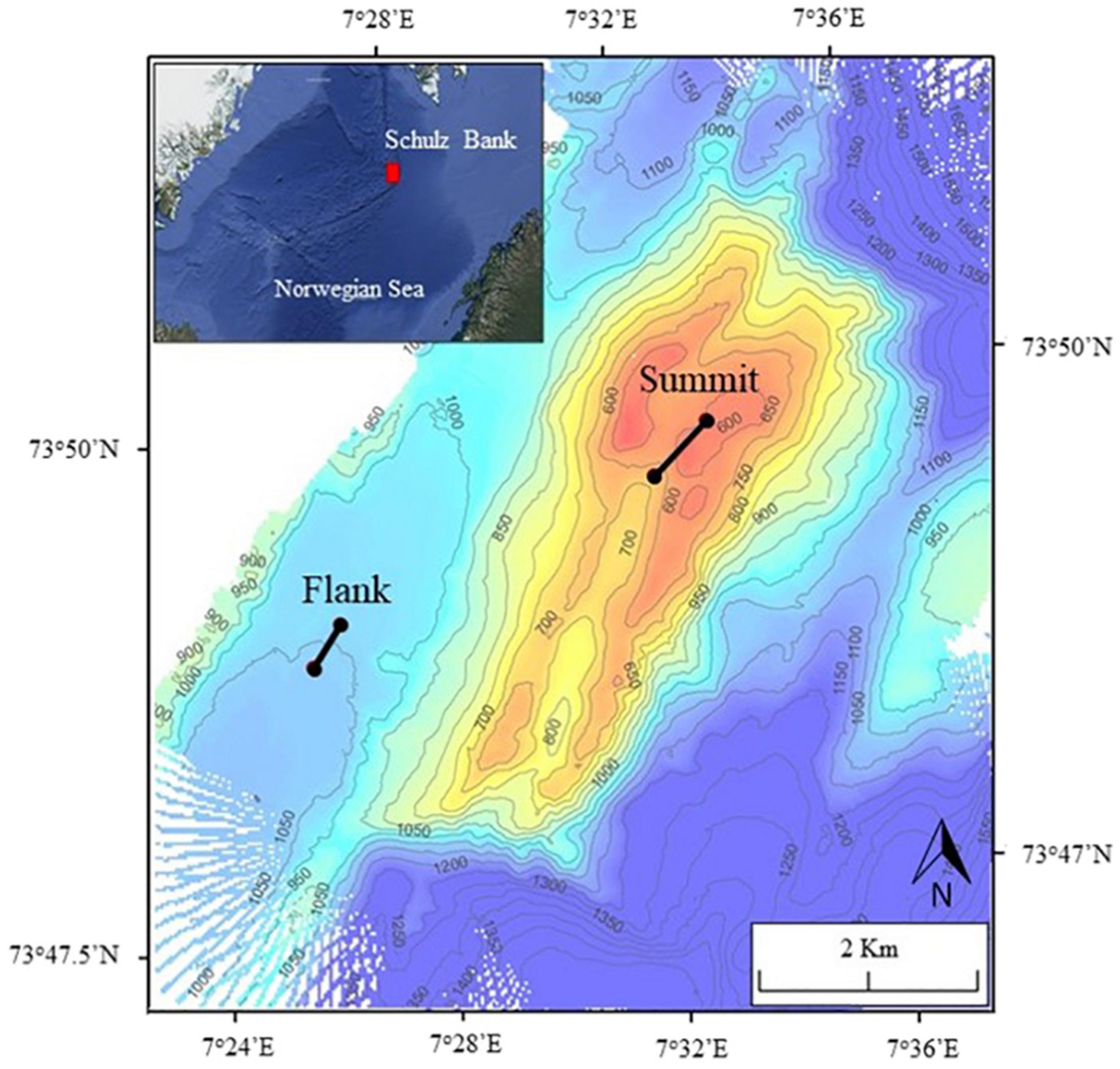
Map of Schulz Bank showing the two Agassiz trawl marks made in 2014. Control transects are located 50 m to the west and east of each trawl mark. The red box in the overview panel highlights the location of Schulz Bank.
Study Design and Data Collection
In 2014, two experimental Agassiz trawls were conducted on the Schulz Bank (Figure 1); one at the summit (568–670 m depth) and one on the southwestern flank (1,464 m depth). The 3-m-wide Agassiz trawl, with a 1 cm mesh size in the cod-end (Figure 2), was towed along the seafloor for 676 m on the summit and 441 m on the flank, resulting in a disturbed area of 2,028 and 1,323 m2, for the summit and flank, respectively. Towing speed was maintained at around 2 knots and the initial and final position were recorded.
FIGURE 2
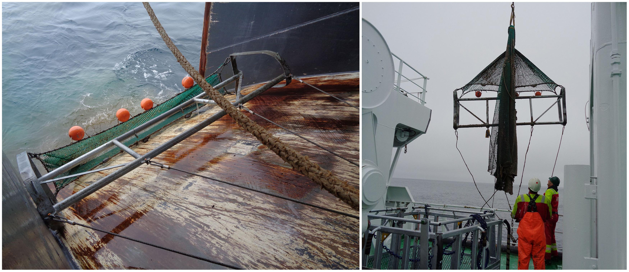
Agassiz trawl used to create physical disturbance on the Schulz Bank.
Although we do not have visual information on the communities inhabiting that specific patch prior to trawling, the densities estimated from the trawl catches suggested that most morphospecies were present in comparable densities compared to neighboring areas (Rapp, H.T, unpublished data). This is further corroborated by the study of Meyer et al. (2019) who found that the distribution of the benthic community in the area is sufficiently homogenous for our purposes.
In August 2018, the two trawl marks and four additional control transects (one on either side of the trawl mark) were surveyed while onboard the R/V G.O.Sars (Table 1). Video recordings were taken along the trawl marks and control transects with the ROV AEGIR6000. Control transects were located 50 m to the east and west of each trawl mark and were performed parallel to the mark. Prior to the collection of video footage, we performed various transects in order to carefully map the trawl marks using the high resolution multibeam mounted on the remotely operated vehicle (ROV). In addition, scrape marks were clearly visible on both sides of the Agassiz trawl transect line, which helped the ROV pilots maintaining the transects.
TABLE 1
| Transect | Start (°N/°E) End (°N/°E) | Avg. depth (m) | Transect area (m2) | Images used | Sampling units | Avg. sampling unit size (m2) | Total area covered (m2) | Transect coverage (%) |
| Summit (August 1, 2018) | ||||||||
| West | 73.8263/7.5376 | 609 (31) | 2082 | 72 | 18 | 16.0 (1.5) | 287 | 13.8% |
| 73.8304/7.5545 | ||||||||
| East | 73.8303/7.5555 | 590 (31) | 2043 | 27 | 8 | 14.3 (1.4) | 114 | 5.6% |
| 73.8261/7.5395 | ||||||||
| Trawl | 73.8262/7.5384 | 605 (31) | 2040 | 64 | 15 | 14.8 (1.5) | 223 | 10.9% |
| 73.8303/7.5547 | ||||||||
| Flank (August 4, 2018) | ||||||||
| West | 73.8159/7.4430 | 1464 (0.1) | 1477 | n/a | 10 | 150 (0.2) | 1477 | 100% |
| 73.8125/7.4340 | ||||||||
| East | 73.8125/7.4352 | 1464 (0.1) | 1417 | n/a | 9 | 150 (0.3) | 1417 | 100% |
| 73.8157/7.4437 | ||||||||
| Trawl | 73.8126/7.4349 | 1464 (0.1) | 1323 | n/a | 9 | 150 (0.3) | 1323 | 100% |
| 73.8158/7.4433 | ||||||||
Details of the 2018 imagery transects recorded on Schulz Bank.
“Images used” shows total numbers of photographs with acceptable quality and covering an area in the 1.5 to 6 m2 range for the summit. Standard deviations are shown in parentheses.
The ROV was equipped with two high-definition HD video cameras (Imenco Spinner Shark Camera HD-SDI camera, 1080p/720p). Only the downward looking camera was used for quantitative ecological data. Two parallel lasers were used as scale (16 cm apart). The ROV was equipped with both ultra-short baseline navigation to provide absolute global position (accuracy approximately ±10 m), and Doppler velocity log navigation (LINKQUEST Doppler log) to provide very accurate relative position (±0.1 m). During every transect the ROV was run in a straight line, on a set bearing, at a constant speed and at the same set altitude (2–3 m).
Image and Video Analysis
From the summit transects, we extracted 287 randomly selected, non-overlapping images (at least 5 m apart). Seafloor images were excluded if (1) the area of the image was less than 1.5 m2 or greater than 6 m2, (2) laser dots were not visible, or (3) the image was obscured by suspended sediment. From the summit, after excluding unusable images, a total of 163 images were used.
All discernable epibenthic megafauna (hereafter referred to as “morphospecies”) greater than 1 cm were counted and identified to the lowest possible taxonomic level in each frame. Fauna that could not be identified to genus or species level were grouped by their size. Unidentifiable demosponges smaller than 10 cm were grouped as “small demosponges,” those between 10 and 20 cm were grouped as “medium demosponges,” and those greater than 20 cm were grouped as “large demosponges.” Schaudinnia rosea, Trichasterina borealis, and Scyphidium septentrionale were grouped as “Hexactinellida spp.” (Meyer et al., 2019). Hexactinellids smaller than 10 cm were grouped as “small Hexactinellida spp.”
For each image, we also measured image area, percent coverage of different substrate types (soft substrate, hard substrate, and spicule mat), and percent coverage of Lissodendoryx complicata which could not be distinguished by individuals, using a grid in IMAGEJ software. Substrate types and fauna were counted in each grid cell and divided by the total number of cells and multiplied by 100 to get percent coverage. Percent coverage of Hexadella dedritifera, an encrusting sponge, was recorded as part of a subsample.
A subsample of 46 random frames taken from our summit samples was used to count highly abundant fauna (Ascidiacea sp. 1 and H. dedritifera), and to assess the sizes (cm2) of the five largest sponge morphospecies on the summit (Geodia parva, Stelletta rhaphidiophora, “large demosponges,” Hexactinellida spp. and Hemigellius sp.).
Single photographs do not represent adequate sampling units because the area of one image is too small to represent benthic communities (Durden et al., 2016). To better represent the community, we chose a desired area based on species accumulation curves (Figure 3) using the “Vegan” package in R statistical software (version 4.0.2; R Core Team, 2017). Data from multiple consecutive images were pooled into “sampling units” that covered segments of transect close to the desired area (ranging between 12.23 and 18.54 m2) (Table 1). In our analyses, “sampling units” have been treated as replicates.
FIGURE 3
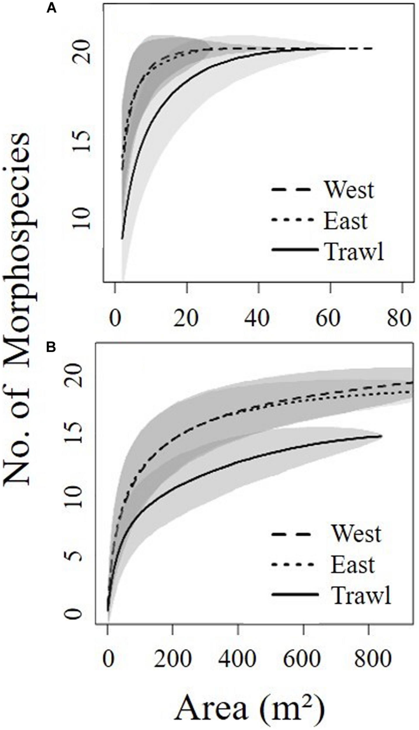
Species accumulation curves for each site determined from seafloor area coverage of the summit (A) and the flank (B) of Schulz Bank. Shaded areas represent 95% confidence intervals. Curves were made using the species accumulation “random” method in “Vegan” package in R statistical software.
The benthic community found in the deeper area was less dense and patchier, therefore we chose to do continuous annotation of the entire transects to quantify sponges and associated fauna to ensure appropriate coverage. We used OFOP software (Ocean Floor Observation Protocol 3.3.7e) (Huetten and Greinert, 2008) to annotate all observations from the three flank transects. Like the summit, all taxa greater than 1 cm were counted and identified to the lowest possible taxonomic level. Accumulation curves (Figure 3) suggested that the observations would be grouped into 28 replicate video segments covering 150 m2 “sampling units” (Table 1). In addition, a subsample of 142 random frames was taken to count ophiuroids, which were highly abundant.
Data Analysis
For each sampling unit, we computed total morphospecies density (individuals m–2) and individual morphospecies densities.
Fishes were excluded from analyses due to their high mobility and, to focus on more abundant and reliably sampled taxa, only data from morphospecies observed at least three times were included in analyses (excluding 20 morphospecies on the summit and 8 on the flank). On the summit 23 morphospecies were used. On the flank 19 morphospecies were used (Supplementary Table 1). Sponge morphospecies were designated as “structural” following ICES (2009) and Beazley et al. (2013). Non-structural sponges and other invertebrates were designated as “associated fauna.” These included sessile cnidarians, echinoderms, ascidians, and encrusting sponges.
To compare the diversity of morphospecies for each treatment (trawled and control transects), several diversity metrics were computed including number of different morphospecies present (S), Shannon diversity index (H’), Simpson’s reciprocal diversity index (1-D), and evenness (J’ and E) using the “Vegan” package in R software (Oksanen et al., 2013). We hypothesize that the communities on the trawled areas will have a lower number of morphospecies (S), Shannon diversity index (H’) and Simpson’s reciprocal diversity index (1-D). However, we expect that both measures of evenness (J’ and E) will be higher inside the trawled areas compared to the control transects (Table 6).
To evaluate if there were significant differences in morphospecies densities and diversity indices between the different transects, we used either a one-way ANOVA following assumptions of normality or Kruskal–Wallis matched pairs test if normality was not met. Normality was tested using the Anderson–Darling normality test. To identify which treatments differed for each site, post hoc tests were performed (Tukey HSD for parametric and Dunn for non-parametric). Significance at the 5% level was reported.
For multivariate community analyses, Bray–Curtis metric was chosen for its capability in handling a large proportion of zeros. Matrices were used in non-metric multidimensional scaling (nMDS) to visualize differences in community composition among transects. The similarity matrices were compared statistically using permutational ANOVA (PERMANOVA, 999 permutations) with pair-wise tests to see statistically significant variations in community composition between treatments. The morphospecies contributing most to dissimilarity between groups were identified using Similarity Percentage (SIMPER) analysis.
Differences in substrate types and in the sizes of the five largest structural sponges between the control and trawled transects were assessed with one-way Kruskal–Wallis tests. Statistical analyses were performed using the computing environment R (version 4.0.2; R Core Team, 2017).
Results
Epibenthic Megafaunal Density and Composition
The epibenthic megafaunal density and composition on the summit and flank of Schulz Bank were visually different (Figure 4). The average densities of morphospecies were significantly different between transects on both the summit and the flank (Summit: Kruskal–Wallis, chi-square = 24.76, df = 2, p < 0.001; Flank: Kruskal–Wallis, chi-square = 16.53, df = 2, p < 0.001). Pairwise comparisons using Dunn post hoc tests showed that the disturbed areas of both sites had significantly lower densities than both control areas (Figure 5).
FIGURE 4
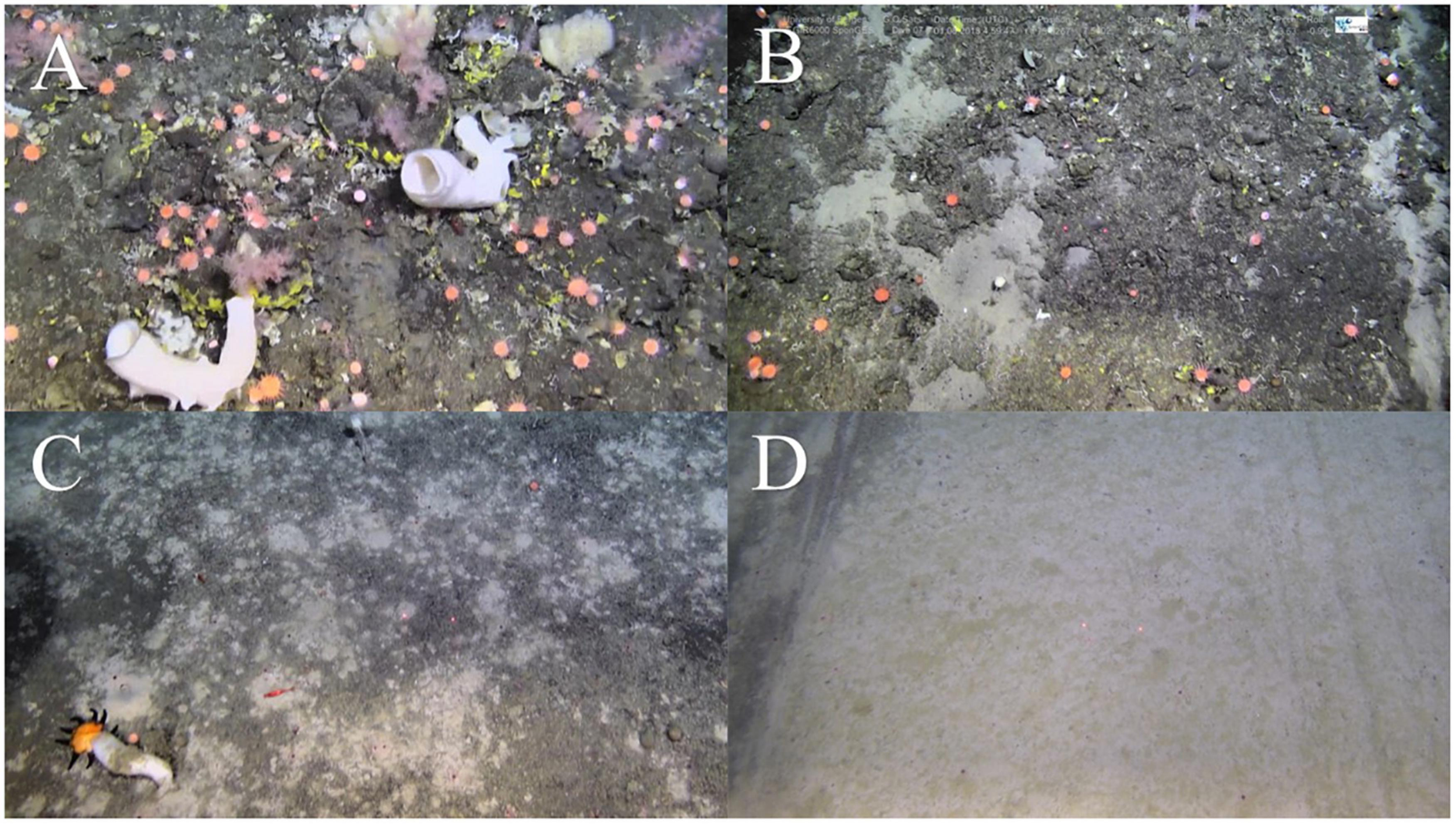
Stills of the epibenthic communities on Schulz Bank; (A) summit control, (B) summit trawl mark (note the exposed soft sediment), (C) flank control, and (D) flank trawl mark.
FIGURE 5
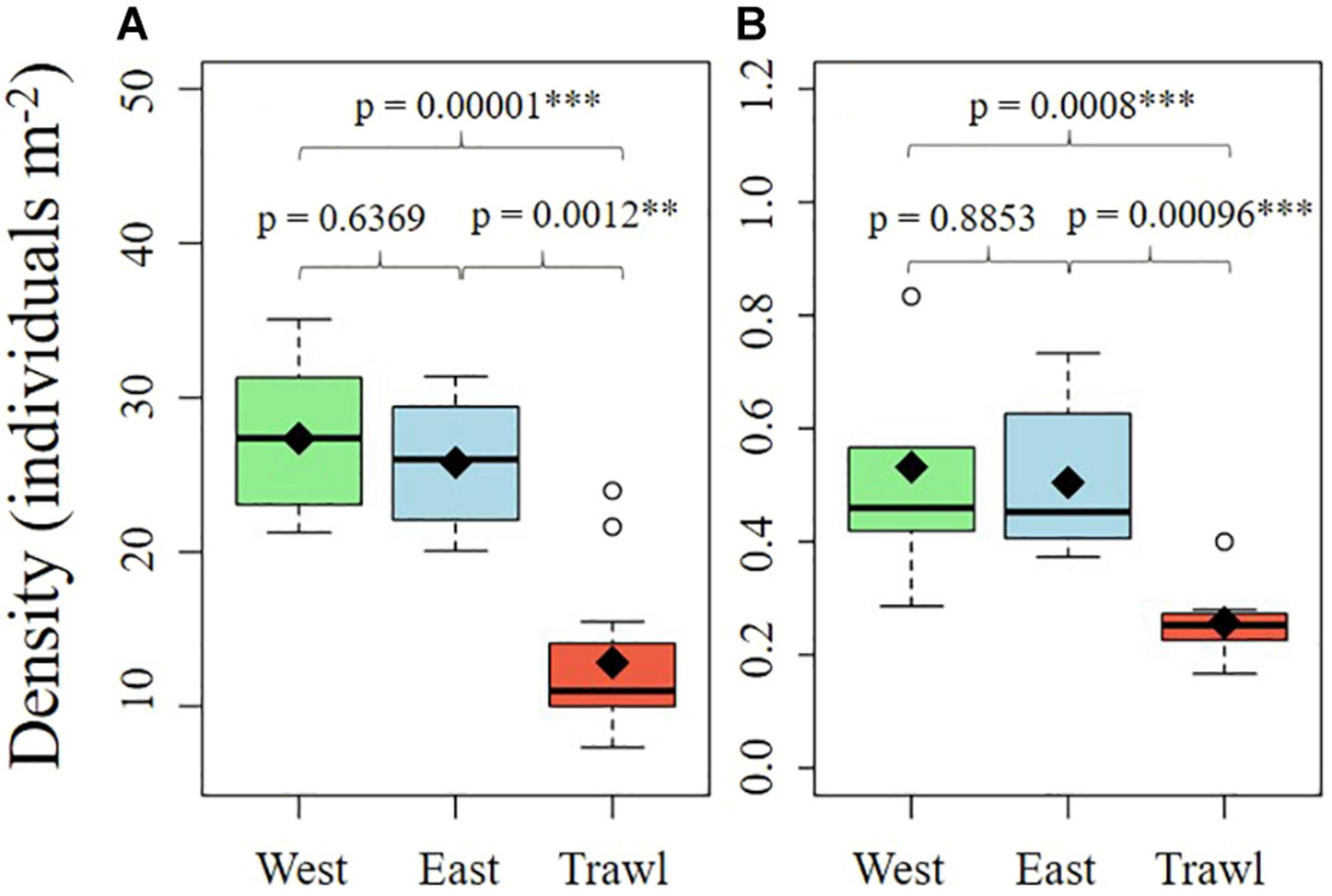
Boxplots of the density of all megafauna found on the summit (A) and the flank (B) of Schulz Bank. Means are noted by diamond shapes.
On the summit, the average density of morphospecies (±SE) on the disturbed site was 12.86 ± 1.19 individuals m–2, compared to 26.6 ± 1.27 in the control areas. On average (± SE), control sites had 6.90 ± 0.51 structural sponges m–2, while trawled areas had an average of 5.18 ± 0.58 structural sponges m–2. The most abundant structural sponges on the summit were “small demosponges” (40% of sponges), Craniella infrequens (24%), G. parva (6%), S. rhaphidiophora (5%), and Hexactinellida spp. (5%). Disturbed areas had significantly less Hexactinellida spp., C. infrequens, Lissodendoryx complicata (Figure 6), Haliclonia sp., and “unidentified demosponge 3” than both control areas (Table 2). For the associated fauna, on average (±SE), control areas had densities of 27.29 ± 1.33 individuals m–2, while trawled areas had an average (±SE) of 10.65 ± 0.99 individuals m–2. Trawled areas had significantly less “unknown demosponge 1,” G. rubiformis, Actiniaria sp., and ascidians than both control areas (Table 2). The encrusting sponge H. dedritifera covered an average of 2% of the area covered on Control West transect but covered significantly less on Control East and trawled transects (Figure 6).
FIGURE 6
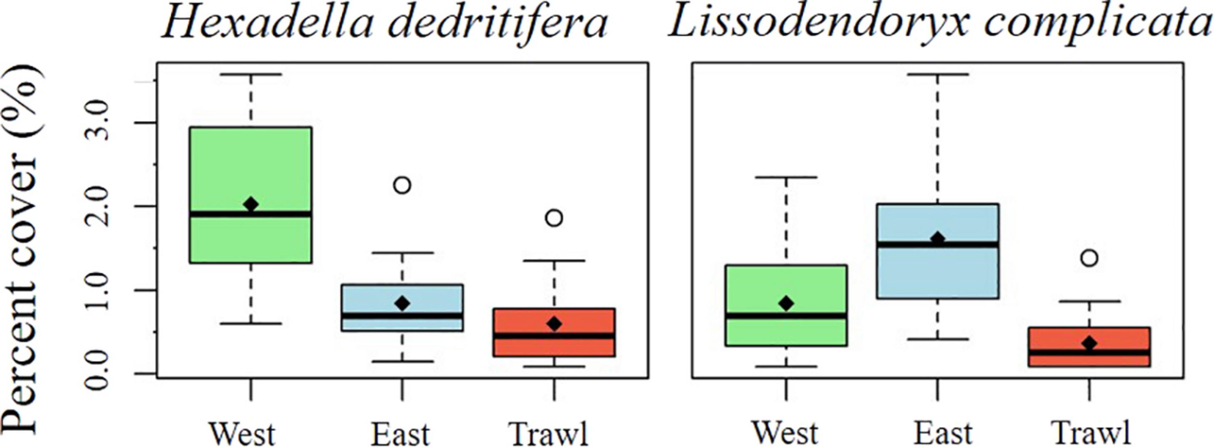
Mean percentage cover of H. dedritifera and L. complicata on the summit of Schulz Bank.
TABLE 2
| Summit densities (individuals m–2) | ||||
| Structural sponges | West | East | Trawl | significance |
| Small Hexactinellida spp. | 0.16 (0.03) | 0.18 (0.07) | 0.06 (0.02) | * |
| Hexactinellida spp. | 0.34 (0.06) | 0.64 (0.19) | 0.07 (0.03) | *** |
| Geodia parva | 0.59 (0.04) | 0.26 (0.05) | 0.12 (0.03) | *** |
| Craniella infrequens | 1.82 (0.09) | 2.31 (0.37) | 0.84 (0.11) | *** |
| Polymastia thielei | 0.06 (0.02) | 0.04 (0.03) | 0.02 (0.01) | • |
| Stylocordyla borealis | 0.07 (0.02) | 0.07 (0.04) | 0.03 (0.01) | • |
| Haliclona sp. | 0.05 (0.01) | 0.09 (0.02) | 0.01 (0.01) | *** |
| Hemigellius sp. | 0.14 (0.02) | 0.13 (0.05) | 0.03 (0.01) | ** |
| Stelletta rhaphidiophora | 0.45 (0.08) | 0.43 (0.09) | 0.21 (0.04) | • |
| Small demosponge | 2.19 (0.15) | 2.87 (0.32) | 3.04 (0.37) | • |
| Medium demosponge | 0.13 (0.03) | 0.15 (0.04) | 0.57 (0.14) | *** |
| Unidentified demosponge 3 | 0.14 (0.04) | 0.13 (0.03) | 0.01 (0.01) | *** |
| Large demosponge | 0.17 (0.03) | 0.25 (0.07) | 0.17 (0.03) | • |
| Total | 6.25 (0.24) | 7.54 (0.77) | 5.18 (0.58) | * |
| Associated fauna | ||||
| Unidentified demosponge 1 | 0.58 (0.06) | 0.41 (0.06) | 0.12 (0.04) | *** |
| Unidentified demosponge 2 | 0.17 (0.03) | 0.04 (0.02) | 0.03 (0.02) | *** |
| Gersemia rubiformis | 3.52 (0.43) | 3.40 (0.44) | 1.34 (0.17) | *** |
| Actiniaria sp. | 16.74 (0.79) | 14.16 (1.50) | 6.08 (0.90) | *** |
| Tylaster willei | 0.04 (0.01) | 0.11 (0.03) | 0.02 (0.01) | ** |
| Hymenaster sp. | 0.03 (0.01) | 0.01 (0.01) | 0.02 (0.01) | • |
| Strongylocentrotus test | 0.06 (0.02) | 0.15 (0.04) | 0.07 (0.01) | • |
| Ascidiacea sp. 1 | 6.91 (0.83) | 8.24 (0.95) | 2.97 (0.64) | *** |
| Total | 28.05 (0.96) | 26.52 (1.7) | 10.65 (0.99) | *** |
Schulz Bank summit mean individuals m–2 (SE) of morphospecies and significance of the difference between transects.
•p > 0.05. *p ≤ 0.05. **p ≤ 0.01. ***p ≤ 0.001.
On the flank, the average density of morphospecies (excluding ophiuroids) on the disturbed site was 0.26 ± 0.02 individuals m–2 (±SE), compared to 0.52 ± 0.06 individuals m–2 (±SE) in the control areas. On average (±SE), control areas contained 0.32 ± 0.05 structural sponges m–2, while trawled areas had an average (±SE) of 0.14 ± 0.02 structural sponges m–2. Trawled areas had significantly less S. borealis, “small demosponges,” and “large demosponges” than both control areas (Table 3). Control areas contained an average (±SE) of 8.91 ± 0.31 associated individuals m–2, while trawled areas had an average (±SE) of 7.46 ± 0.34 associated individuals m–2. The most abundant associated fauna was ophiuroids, which averaged 8.72 ± 0.30 individuals m–2 (±SE) in control areas and 7.35 ± 0.33 individuals m–2 (±SE) in trawled areas. Ophiuroids comprised 98% of all associated individuals, followed by Actiniaria sp. (1%). Trawled areas had significantly less Actiniaria sp. than both control areas (Table 3).
TABLE 3
| Flank densities (individuals m–2) |
||||
| Structural sponges | West | East | Trawl | significance |
| Hexactinellida spp. | 0.016 (0.006) | 0.010 (0.003) | 0.002 (0.002) | * |
| Geodia hentscheli | 0.003 (0.002) | 0.001 (0.001) | 0 | • |
| Craniella infrequens | 0.049 (0.012) | 0.041 (0.008) | 0.024 (0.007) | • |
| Stylocordyla borealis | 0.195 (0.055) | 0.181 (0.041) | 0.082 (0.016) | * |
| Lycopodina sp. | 0.014 (0.003) | 0.045 (0.009) | 0.030 (0.006) | ** |
| Haliclona sp. | 0.003 (0.001) | 0 | 0 | * |
| Small demosponge | 0.022 (0.004) | 0.039 (0.007) | 0.002 (0.002) | *** |
| Medium demosponge | 0.003 (0.002) | 0.008 (0.003) | 0.004 (0.004) | * |
| Large demosponge | 0.006 (0.002) | 0.007 (0.003) | 0 | * |
| Total | 0.311 (0.058) | 0.331 (0.051) | 0.144 (0.022) | ** |
| Associated fauna | ||||
| Actiniaria sp. | 0.105 (0.010) | 0.090 (0.011) | 0.033 (0.006) | *** |
| Umbellula sp. | 0.002 (0.001) | 0.001 (0.001) | 0.001 (0.001) | • |
| Bythocaris sp. | 0.017 (0.004) | 0.010 (0.002) | 0.010 (0.003) | • |
| Scalpellidae indet. | 0.012 (0.006) | 0.006 (0.003) | 0.004 (0.001) | • |
| Feather star | 0.001 (0.001) | 0.002 (0.001) | 0.001 (0.001) | • |
| Asteroidea sp. | 0.040 (0.005) | 0.027 (0.004) | 0.047 (0.009) | • |
| Solaster sp. | 0.002 (0.001) | 0.002 (0.001) | 0 | • |
| Ophiuroid | 7.905 (0.265) | 9.551 (0.332) | 7.352 (0.327) | *** |
| Ascidiacea sp. 1 | 0.009 (0.003) | 0.010 (0.003) | 0.002 (0.002) | • |
| Ascidiacea sp. 2 | 0.007 (0.004) | 0.006 (0.003) | 0.001 (0.001) | • |
| Total | 8.105 (0.265) | 9.706 (0.344) | 7.456 (0.337) | *** |
Schulz Bank flank mean individuals m–2 (SE) of morphospecies and significance of the difference between transects.
•p > 0.05. *p ≤ 0.05. **p ≤ 0.01. ***p ≤ 0.001.
Taxonomic Richness and Diversity
Summit
The number of different morphospecies present (S) significantly differed between summit transects (Kruska—Wallis; chi-square = 17.01, df = 2, p < 0.001). There were significantly less morphospecies in the trawled area. On the summit, the trawled area had an average (±SE) of 12.20 ± 0.52 morphospecies present, while control areas had an average (±SE) of 15.65 ± 0.54 morphospecies present. Simpson’s Diversity index (1-D) differed between summit transects (Kruskal–Wallis; chi-square = 12.61, df = 2, p < 0.01). In the trawl and Control East areas, there was a lower probability that two random individuals belonged to different morphospecies, indicating lower diversity than in the Control West area. Evenness (E) also differed between transects on the summit (Kruskal–Wallis; chi-square = 18.63, df = 2, p < 0.001). Trawling significantly increased the evenness of summit morphospecies (Table 4).
TABLE 4
| Site | Transect | Total average density (individuals m–2) | S mean (SE) | H′ mean (SE) | 1-D mean (SE) | J′ mean (SE) | E mean (SE) |
| Summit | West | 34.30 | 15.39 (0.49) | 1.42 (0.03) | 0.41 (0.01) | 0.52 (0.01) | 0.92 (0.03) |
| East | 34.06 | 15.88 (0.58) | 1.55 (0.07) | 0.35 (0.03) | 0.56 (0.02) | 1.10 (0.09) | |
| Trawl | 15.83 | 12.20 (0.52) | 1.52 (0.04) | 0.32 (0.02) | 0.61 (0.02) | 1.30 (0.06) | |
| Flank | West | 8.42 | 11.70 (0.52) | 1.84 (0.04) | 0.24 (0.03) | 0.75 (0.03) | 1.93 (0.21) |
| East | 10.04 | 11.67 (0.60) | 1.88 (0.08) | 0.23 (0.03) | 0.77 (0.03) | 1.99 (0.18) | |
| Trawl | 7.60 | 7.78 (0.40) | 1.70 (0.04) | 0.23 (0.01) | 0.83 (0.02) | 2.19 (0.10) |
Characteristics of transects on Schulz Bank.
For each transect: density of total epibenthic megafauna, number of morphospecies present (S), Shannon Weaver diversity index (H′), Simpson’s reciprocal index (1-D), Pielou’s evenness (J′), and evenness derived from 1/D (E).
Flank
The number of different morphospecies present (S) significantly differed between transects on the flank (Kruskal–Wallis; chi-square = 16.66, df = 2, p < 0.001). There were fewer morphospecies within trawled areas. Control transects had an average (±SE) of 11.69 ± 0.56 morphospecies present while the trawled area had an average (±SE) of 7.78 ± 0.40 morphospecies present. Simpson’s Diversity index (1-D) did not differ between flank transects (Kruskal–Wallis; chi-square = 1.07, df = 2, p > 0.5). Evenness (E) also did not differ between flank transects (Kruskal–Wallis; chi-square = 1.22, df = 2, p > 0.5). The morphospecies on the flank were more even than those on the summit (Table 4).
Multivariate Community Analyses
Summit
For the summit, the nMDS plot showed strong separation between megafaunal communities in trawled and control areas (Figure 7). Pairwise PERMANOVA tests revealed significant differences between the transects, with trawling explaining 42% of the variation between Control East and Trawl transects, and 58% of the variation between Control West and Trawl transects (Table 5). SIMPER results revealed that the dissimilarity in community composition between Control and Trawl transects was principally driven by Actiniaria sp., G. rubiformis, C. infrequens, “small demosponges,” and Hexactinellida spp. (Table 5).
FIGURE 7
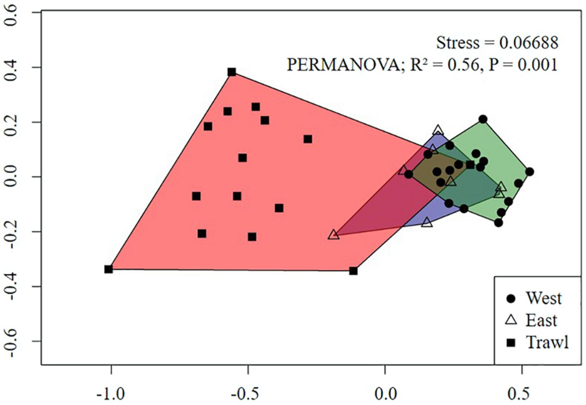
Non-metric Multidimensional Scaling (nMDS) of replicate sampling units for each summit transect on Schulz Bank using Bray-Curtis dissimilarity metric. Each point represents a sampling unit and each polygon represents a transect. Morphospecies abundance values were standardized to individuals m–2.
TABLE 5
| PERMANOVA | SIMPER (% contribution) | |||||
| Test | R2 (P-value) | #1 | #2 | #3 | #4 | #5 |
| Summit | ||||||
| Trawl vs. West | 0.58 (0.002) | Actiniaria sp. (27.4%) | G. rubiformis (5.5%) | Small demosponge (3.5%) | C. infrequens (2.6%) | Demosponge 1 (1.2%) |
| Trawl vs. East | 0.42 (0.002) | Actiniaria sp. (22.2%) | G. rubiformis (5.4%) | C. infrequens (4.1%) | Small demosponge (3.4%) | Hexactinellida spp. (1.6%) |
| Flank | ||||||
| Trawl vs. West | 0.29 (0.002) | S. borealis (14.3%) | Actiniaria sp. (10%) | C. infrequens (5%) | Asteroidea sp. (3.2%) | Small demosponge (2.9%) |
| Trawl vs. East | 0.31 (0.002) | S. borealis (14.1%) | Actiniaria sp. (8.7%) | Small demosponge (5%) | Lycopodina sp. (3.6%) | Asteroidea sp. (3.6%) |
Pairwise PERMANOVA and SIMPER results for densities on the Schulz Bank.
“SIMPER (% contribution)” are ordered by importance (#1 being the most important morphospecies driving differences between transects).
Flank
For the flank, the nMDS plot also showed a strong difference between megafaunal communities in trawled and control areas (Figure 8). Pairwise PERMANOVA tests revealed significant differences between transects, with trawling explaining about 30% of the variation between Control and Trawl transects (Table 5). On the flank, dissimilarity was driven by S. borealis, Actiniaria sp., C. infrequens, “small demosponges,” Lycopodina sp., and Asteroidea sp. (Table 5).
FIGURE 8
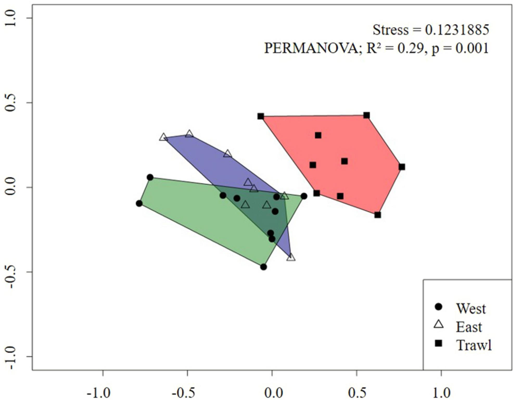
Non-metric Multidimensional Scaling (nMDS) of replicate sampling units for each flank transect on Schulz Bank using Bray-Curtis dissimilarity metric. Each point represents a sampling unit and each polygon represents a transect. Morphospecies abundance values were standardized to individuals m–2.
Size of Large Sponges
Overall, the sizes of the largest sponge morphospecies (G. parva, Hemigellius sp., Hexactinellida spp., “large demosponges,” and S. rhaphidiophora) did not differ between control and trawled transects on the summit. However, Dunn post hoc tests did reveal that G. parva in Control East were significantly larger than those within the trawl mark, and S. rhaphidiophora in Control East were larger than those in both Control West and the trawl mark.
Substrate Cover
On the summit, substrate cover was significantly different between control and disturbed transects (Kruskal–Wallis; chi-square = 26.04, df = 2, p < 0.001). On the control sites, spicule mat dominated the substrate (99.5 and 100% of substrate), but on the disturbed site, there was significantly higher coverage of soft sediment. On the other hand, the flank had no significant differences in substrate type between the disturbed and control areas, being all exclusively composed of soft sediment.
Discussion
This is the first study looking at recovery of Arctic sponge grounds following physical disturbance. Our results provide useful insight on how the diversity and megafaunal composition of sponge-dominated communities can be affected by anthropogenic activities like trawling. Overall, our results suggest that after four years, benthic communities within trawl marks have not returned to a pre-disturbed state (represented by the control transects) with overall densities of epibenthic morphospecies being significantly lower in the disturbed sites than in nearby control areas. One unavoidable limitation of this study was our lack of true replicates for both trawled areas, implying that are sampling units our essentially pseudo-replicates.
Although many structural sponge morphospecies found on the summit were significantly less abundant within the trawl mark than in control areas, we still observed some large sponges in the disturbed area (Table 6). It is likely that these individuals survived the Agassiz trawl in 2014 and are unlikely to be new growth since deep-sea sponges typically have slow growth rates (Leys and Lauzon, 1998; Fallon et al., 2010). Fallon et al. (2010) found that Antarctic deep-sea hexactinellid sponges have extremely long life expectancies (∼440 years). Similarly, Leys and Lauzon found longevities of another deep-sea hexactinellid (Rhabdocalyptus dawsoni, Lamb 1892) to be over 200 years old. Bottom trawls are not 100% selective and occasionally bounce off the seabed, explaining the presence of such large individuals within the trawled area. Moran and Stephenson (2000) studied the effects of otter trawling on macrobenthic invertebrates (>20 cm) and found that a single trawl pass reduced density by only 15.5%. In a similar study, Wassenberg et al. (2002) quantified the direct effects of experimental bottom trawls on sponges and found that selectivity varied based on sponge morphology and size. They found that 30% of large (>500 mm high) globular sponges and 60% of large branched sponges survived trawling. Sainsbury et al. (1992) found that a single trawl pass removed 90% of large sponges. Looking at these studies, the catchability of large sponges by bottom trawls is highly variable, so it is not surprising that we found occasional large sponges in the disturbed area even though Agassiz trawls are among the most efficient types of trawls for sampling benthic communities. Another explanation for the presence of large sponges in the disturbed area comes from video observations obtained from a benthic lander on a Scotian Shelf sponge ground during severe hydrodynamic ‘storm’ events revealing that large Hexactinellid sponges can be dislodged and transported by currents (Hanz et al., 2020). The Schulz Bank summit is made dynamic by strong internal waves at the water mass boundary (Roberts et al., 2018) perhaps capable of rolling sponges around.
TABLE 6
| Summit |
Flank |
||||
| Expected Change | Observed Change | Expected Change | Observed Change | ||
| Density | West v Trawl | Decrease | Decrease | Decrease | Decrease |
| East v Trawl | Decrease | Decrease | Decrease | Decrease | |
| Taxonomic Richness (S) | West v Trawl | Decrease | Decrease | Decrease | Decrease |
| East v Trawl | Decrease | Decrease | Decrease | Decrease | |
| Diversity | West v Trawl | Decrease | Decrease | Decrease | No change |
| East v Trawl | Decrease | No change | Decrease | No change | |
| Evenness | West v Trawl | Increase | Increase | Increase | No change |
| East v Trawl | Increase | Increase | Increase | No change | |
| PERMANOVA | West v Trawl | Strong separation | Strong separation | Strong separation | Strong separation |
| East v Trawl | Strong separation | Strong separation | Strong separation | Strong separation | |
| Sizes of large sponges | West v Trawl | Smaller size | No change | N/A | N/A |
| East v Trawl | Smaller size | No change | N/A | N/A | |
| Substrate cover | West v Trawl | Less spicule mat | Less spicule mat | N/A | N/A |
| East v Trawl | Less spicule mat | Less spicule mat | N/A | N/A | |
Expected versus observed changes on the Schulz Bank.
Changes are what we expected/observed to happen in trawl marks compared to the controls.
We observed a decrease in the density of many associated fauna in the disturbed area, either due to direct removal (Grassle, 1977; Clarke, 1982) or indirectly by the loss of biogenic habitat provided by the sponges (Klitgaard, 1995; Barrio Froján et al., 2012). Associated fauna have been demonstrated to be more abundant and diverse in and around large and structurally complex sponges compared to nearby areas without sponges (Wendt et al., 1985; Kunzmann, 1996). Sponges serve numerous functional roles which benefit other species (Bell, 2008; Buhl-Mortensen et al., 2010). Sessile invertebrates on the summit, which are abundant in control areas, like anthozoans and ascidians, were found in low abundances four years after disturbance, possibly due to the loss of preferred settlement substrate. On our summit trawl mark, where we found a significant reduction of spicule mat compared to control areas, a full recovery for many associated fauna and sponge species probably relies on sponge growth and formation of a dense spicule mat (Bett and Rice, 1992). Spicule mats likely take generations of sponges to accumulate and are known to influence macrofaunal community structure and diversity (Barrio Froján et al., 2012; Beazley et al., 2013). Roberts et al. (2018) suggested that the summit of Schulz Bank had provided suitable substrate for sponge settlement and, since initial recruitment, a 20 cm thick spicule mat has been deposited, which is also likely to be beneficial to the formation of a diverse benthic community. Because structure-forming sponges create important biogenic habitat, the loss of these large sponge species can lead to a decrease in biodiversity and changes in community structure (Tissot et al., 2006; Buhl-Mortensen et al., 2010; Beazley et al., 2013; Maldonado et al., 2017).
It is important to highlight that the observed differences in spicule mat cover between the disturbed site and control transects should also explain why we found some sponges at a higher or similar abundance inside the trawl mark compared to the control transects. Meyer et al. (2019) noted that demosponges within the spicule mat can appear hidden. Therefore, in such a dense community, it is likely that we were unable to detect all of the demosponges within the spicule mat, thus leading to underestimation of sponges in the control transects.
Overall, the flank has lower megafaunal density than the summit because as depth increases, the benefits brought by the water mass boundary and internal waves near the summit decrease (Roberts et al., 2018), however the effect of trawling was similar. Like the summit, four years after disturbance, epibenthic megafaunal densities on the flank were significantly lower within the trawl mark than in control areas. Compared to the summit, structural sponges on the flank seemed sparse, with only a few large sponges every 100 m2 of seafloor. A closer look showed that the flank is dotted with many small structural sponges (e.g., Stylocordyla borealis, C. infrequens, Lycopodina sp.). Although this habitat is clearly less diverse and dense, it supports sponge species not seen (or rarely seen) on the summit, like Lycopodina sp. and Geodia hentscheli. Trawling significantly reduced the overall abundance of structural sponges at this site, where they will likely take decades to recover due to their life history traits (Leys and Lauzon, 1998; Gatti, 2002; Fallon et al., 2010). The most abundant sponge, S. borealis, has relatively slow growth rates with average individuals being about 10 years old and the oldest individuals reaching 170 years (Gatti, 2002).
As for associated fauna, the flank was covered with thousands of ophiuroids and, in lower densities, other morphospecies rarely seen on the summit, such as Umbellula sp., Bythocaris sp., and feather stars. The overall abundance of associated fauna on the deep flank was significantly reduced by trawling. But individually, only Actiniaria sp. continued to be affected by trawling four years later. The rest of the associated fauna remained unaffected by the trawl mark, whether this was due to a full recovery or avoidance of the Agassiz trawl is unknown. Mobile epifaunal invertebrates like sea stars and ophiuroids are less affected by trawling, and we did not see any recolonization by organisms taking advantage of the empty space as is sometimes reported for areas once disturbed by bottom contact fishing gear (Engel and Kvitek, 1998; Hixon and Tissot, 2007).
The effect of disturbance on each morphospecies varies depending on their individual selectivity by the gear, their size, resilience, and life history characteristics (Thrush and Dayton, 2002; Williams et al., 2010; Clark et al., 2015). Five years after fishery closures on Tasmanian seamounts, Althaus et al. (2009) saw no recovery in deep coral fauna but found that some resilient species had higher abundances than on actively trawled seamounts. Certain traits, such as small size, flexibility, and mass colonization potentially make some species resilient to physical disturbance (Clark et al., 2010). For example, on the summit, S. borealis did not significantly differ between trawl and control transects. S. borealis is a relatively small, stalked, and flexible species. Although not every individual morphospecies is negatively affected in our study, we saw a clear difference between trawled and untrawled communities overall.
Few studies have investigated the recovery of large sponges after trawling. Van Dolah et al. (1987) found that one year after a single experimental trawl pass in a shallow, hard-bottom habitat, large sponges were able to recover greater than their pre-trawl densities. This is not the case in cold, deep-water systems; Malecha and Heifetz (2017) found that a single trawl pass continued to affect large sponges 13 years after disturbance in the Gulf of Alaska (200 m depth). Their trawled sites had 31.7% lower sponge densities and 58.8% higher rates of injury than in reference areas. Another study in Alaska by Rooper et al. (2011) used sponge catch data and logistic population models to estimate growth and recovery rates. They estimated that large deep-sea sponges would take between 13 and 36 years to recover 80% of their original biomass post trawling. These studies provide evidence for slow recovery of deep-sea sponge grounds following physical disturbance.
Our observations and the life history strategies typical of cold water, deep-sea fauna (Grassle and Sanders, 1973; Dayton, 1979; Clarke, 1980; Leys and Lauzon, 1998; Sarà et al., 2002; Young, 2003; Fallon et al., 2010) suggest that four years is not enough for a community on the Schulz Bank to recover from a trawling disturbance. Recovery of disturbed communities in these locations, especially on the summit, will likely take decades to centuries.
The amount and intensity of disturbance is an important factor influencing recovery. Multiple trawls through Schulz Bank sites would have likely caused greater damage to the communities, significantly delaying recovery, as seen in studies where the indirect effects of repeated trawling continue to influence deep benthic communities long after disturbance (Koslow et al., 2001; Althaus et al., 2009; Williams et al., 2010; Clark et al., 2019). In the present study, the small disturbed area benefited from a neighboring healthy benthic community, facilitating re-colonization, which is not the case for large fishing grounds, where pristine populations are located sometimes far away.
Overall, this study provides a quantitative snapshot of the status of a sponge-dominated community of the Arctic four years after being impacted by a bottom trawl and marks the beginning in following its recovery trajectory. This new information, which suggests a slow recovery rate, is important in promoting the conservation of this diverse and sensitive ecosystem. It also provides an evidence-based threat evaluation for a VME, of relevance for other sponge ground ecosystems of the deep sea. We encourage regular monitoring of the area to fully quantify and characterize complete recovery processes of this ecosystem. The remoteness and absence of direct human activities makes the area a perfect case-study for the understanding of recovery dynamics of deep-sea sponge ecosystems following impacts. Future studies would benefit from higher resolution cameras in combination with the collection of physical samples to enable the quantification of small, recently settled sponges.
Statements
Data availability statement
The original contributions presented in the study are included in the article/Supplementary Material, further inquiries can be directed to the corresponding author.
Author contributions
CP and KM conceived and carried out the study. HM, ER, and HR advised on identification of species and analysis methods. KM analyzed the data, wrote the manuscript, and prepared the figures. All authors revised drafts of the manuscript and gave final approval for publication.
Funding
The work leading to this publication has received funding from the European Union’s Horizon 2020 Research and Innovation Programme through the SponGES project (grant agreement No 679849). This document reflects only the authors’ view and the Executive Agency for Small and Medium-sized Enterprises (EASME) is not responsible for any use that may be made of the information it contains.
Acknowledgments
Thanks are due to the SponGES team for their guidance, advice on our study design, and help with epifaunal morphospecies identification in the image data. Thanks to the IMAR staff for providing office space and resources. And thanks to the G.O.Sars crew, AEGIR6000 crew, and science team that carried out the ROV surveys. Finally, we would like to dedicate this contribution to our friend and colleague Hans Tore Rapp.
Conflict of interest
The authors declare that the research was conducted in the absence of any commercial or financial relationships that could be construed as a potential conflict of interest.
Supplementary material
The Supplementary Material for this article can be found online at: https://www.frontiersin.org/articles/10.3389/fmars.2020.605281/full#supplementary-material
References
1
Althaus F. Williams A. Schlacher T. A. Kloser R. J. Green M. A. Barker B. A. et al (2009). Impacts of bottom trawling on deep-coral ecosystems of seamounts are long-lasting.Mar. Ecol. Prog. Ser.397279–294. 10.3354/meps08248
2
Amsler M. O. Mcclintock J. B. Amsler C. D. Angus R. A. Baker B. J. (2009). An evaluation of sponge-associated amphipods from the Antarctic Peninsula.Antarct. Sci.21579–589. 10.1017/s0954102009990356
3
Barrio Froján C. R. Bolam S. G. Eggleton J. D. Mason C. (2012). Large-scale faunal characterisation of marine benthic sedimentary habitats around the UK.J. Sea Res.6953–65. 10.1016/j.seares.2012.02.005
4
Barthel D. (1992). Do hexactinellids structure Antarctic sponge associations?Ophelia36111–118. 10.1080/00785326.1992.10430362
5
Beazley L. I. Kenchington E. L. Murillo F. J. Sacau M. D. M. (2013). Deep-sea sponge grounds enhance diversity and abundance of epibenthic megafauna in the Northwest Atlantic.ICES J. Mar. Sci.701471–1490. 10.1093/icesjms/fst124
6
Bell J. J. (2008). The functional roles of marine sponges.Estuar.Coast. Shelf Sci.79341–353. 10.1016/j.ecss.2008.05.002
7
Bell J. J. McGrath E. Biggerstaff A. Bates T. Bennett H. Marlow J. et al (2015). Sediment impacts on marine sponges.Mar. Pollut. Bull.945–13. 10.1016/j.marpolbul.2015.03.030
8
Bett B. J. Rice A. L. (1992). The influenceof hexactinellid sponge (Pheronema carpenteri) spicules on the patchy distribution of macrobenthos in the Porcupine seabight (bathyal ne atlantic).Ophelia36217–226. 10.1080/00785326.1992.10430372
9
Buhl-Mortensen L. Vanreusel A. Gooday A. J. Levin L. A. Priede I. G. Buhl-Mortensen P. et al (2010). Biological structures as a source of habitat heterogeneity and biodiversity on the deep ocean margins.Mar. Ecol.3121–50. 10.1111/j.1439-0485.2010.00359.x
10
Carreiro-Silva M. Andrews A. H. Braga-Henriques A. De Matos V. Porteiro F. M. Santos R. S. (2013). Variability in growth rates of long-lived black coral Leiopathes sp. from the Azores.Mar. Ecol. Prog. Ser.473189–199. 10.3354/meps10052
11
Clark M. R. Althaus F. Schlacher T. A. Williams A. Bowden D. A. Rowden A. A. (2015). The impacts of deep-sea fisheries on benthic communities: a review.ICES J. Mar. Sci.73(Suppl._1), i51–i69.
12
Clark M. R. Bowden D. A. Rowden A. A. Stewart R. (2019). Little evidence of benthic community resilience to bottom trawling on seamounts after 15 years.Front. Mar. Sci.6:63. 10.3389/fmars.2019.00063
13
Clark M. R. Rowden A. A. (2009). Effect of deepwater trawling on the macro-invertebrate assemblages of seamounts on the Chatham Rise, New Zealand.Deep Sea Res. Part I Oceanogr. Res. Pap.561540–1554. 10.1016/j.dsr.2009.04.015
14
Clark M. R. Rowden A. A. Schlacher T. Williams A. Consalvey M. Stocks K. I. et al (2010). The ecology of seamounts: structure, function, and human impacts.Annu. Rev. Mar. Sci.2253–278. 10.1146/annurev-marine-120308-081109
15
Clarke A. (1980). A reappraisal of the concept of metabolic cold adaptation in polar marine invertebrates.Biol. J. Linn. Soc.1477–92. 10.1111/j.1095-8312.1980.tb00099.x
16
Clarke A. (1982). Temperature and embryonic development in polar marine invertebrates.Int. J. Invertebr. Reprod.571–82. 10.1080/01651269.1982.10553456
17
Cook S. E. Conway K. W. Burd B. (2008). Status of the glass sponge reefs in the Georgia Basin.Mar. Environ. Res.66S80–S86.
18
Dayton P. K. (1979). Observations of growth, dispersal and population dynamics of some sponges in McMurdo Sound. Antarctica.Colloques Internationaux du CNRS291271–282.
19
Durden J. M. Schoening T. Althaus F. Friedman A. Garcia R. Glover A. G. et al (2016). Perspectives in visual imaging for marine biology and ecology: from acquisition to understanding.Oceanogr. Mar. Biol.541–72. 10.1201/9781315368597-2
20
Engel J. Kvitek R. (1998). Effects of otter trawling on a benthic community in Monterey Bay National Marine Sanctuary.Conserv. Biol.121204–1214. 10.1046/j.1523-1739.1998.0120061204.x
21
Fallon S. J. James K. Norman R. Kelly M. Ellwood M. J. (2010). A simple radiocarbon dating method for determining the age and growth rate of deep-sea sponges.Nuclear Instrum. Methods Phys. Res. Sect. B Beam Interact. Mater. Atoms2681241–1243. 10.1016/j.nimb.2009.10.143
22
FAO (2009). International Guidelines for the Management of Deep-Sea Fisheries in the High Seas.Rome: FAO.
23
Fosså J. H. Mortensen P. B. Furevik D. M. (2002). The deep-water coral Lophelia pertusa in Norwegian waters: distribution and fishery impacts.Hydrobiologia4711–12.
24
Freese J. L. Wing B. L. (2003). Juvenile red rockfish. Sebastes sp., associations with sponges in the Gulf of Alaska.Mar. Fish. Rev.6538–42.
25
Freese L. Auster P. J. Heifetz J. Wing B. L. (1999). Effects of trawling on seafloor habitat and associated invertebrate taxa in the Gulf of Alaska.Mar. Ecol. Prog. Ser.182119–126. 10.3354/meps182119
26
Gatti S. (2002). The rôle of sponges in high-Antarctic carbon and silicon cycling-a modelling approach= Die Rolle der Schwämme im hochantarktischen Kohlenstoff-und Silikatkreislauf-ein Modellierungsansatz.Berichte zur Polar Meeresforschung434:124.
27
Goode S. L. Rowden A. A. Bowden D. A. Clark M. R. (2020). Resilience of seamount benthic communities to trawling disturbance.Mar. Environ. Res.161:105086. 10.1016/j.marenvres.2020.105086
28
Grant N. Matveev E. Kahn A. S. Archer S. K. Dunham A. Bannister R. J. et al (2019). Effect of suspended sediments on the pumping rates of three species of glass sponge in situ.Mar. Ecol. Prog. Ser.61579–100. 10.3354/meps12939
29
Grassle J. F. (1977). Slow recolonisation of deep-sea sediment.Nature265618–619. 10.1038/265618a0
30
Grassle J. F. Sanders H. L. (1973). Life histories and the role of disturbance.Deep Sea Res. Oceanogr. Abstracts20643–659. 10.1016/0011-7471(73)90032-6
31
Hanz U. Beazley L. I. Kenchington E. Duineveld G. Rapp H. T. Mienis F. (2020). Seasonal variability in near-bed environmental conditions in the Vazella pourtalesii glass sponge grounds of the Scotian Shelf.Front. Marine Sci.
32
Hawkes N. Korabik M. Beazley L. Rapp H. T. Xavier J. R. Kenchington E. (2019). Glass sponge grounds on the scotian shelf and their associated biodiversity.Mar. Ecol. Prog. Ser.61491–109. 10.3354/meps12903
33
Hixon M. A. Tissot B. N. (2007). Comparison of trawled vs untrawled mud seafloor assemblages of fishes and macroinvertebrates at Coquille Bank, Oregon.J. Exp. Mar. Biol. Ecol.34423–34. 10.1016/j.jembe.2006.12.026
34
Hogg M. M. Tendal O. S. Conway K. W. Pomponi S. A. van Soest R. W. M. Gutt J. et al (2010). Deep-sea Sponge Grounds: Reservoirs of Biodiversity.UNEP-WCMC Biodiversity Series No. 32. Cambridge: UNEP-WCMC.
35
Howell K. L. Piechaud N. Downie A. L. Kenny A. (2016). The distribution of deep-sea sponge aggregations in the North Atlantic and implications for their effective spatial management.Deep Sea Res. Part I Oceanogr. Res. Pap.115309–320. 10.1016/j.dsr.2016.07.005
36
Huetten E. Greinert J. (2008). “Software controlled guidance, recording and postprocessing of seafloor observations by ROV and other towed devices: the software package OFOP,” in Geophysical Research Abstracts, EGU2008-A-03088, EGU General Assembly 2008 (poster), Vol. 10Vienna.
37
ICES (2009). Report of the ICES–NAFO Working Group on Deep-Water Ecology (WGDEC). ICES CM 2009ACOM:23, 94.
38
Kaiser M. J. Ramsay K. Richardson C. A. Spence F. E. Brand A. R. (2000). Chronic fishing disturbance has changed shelf sea benthic community structure.J. Anim. Ecol.69494–503. 10.1046/j.1365-2656.2000.00412.x
39
Kenchington E. Power D. Koen-Alonso M. (2013). Associations of demersal fish with sponge grounds on the continental slopes of the northwest Atlantic.Mar. Ecol. Prog. Ser.477217–230. 10.3354/meps10127
40
Klitgaard A. B. (1995). The fauna associated with outer shelf and upper slope sponges (Porifera, Demospongiae) at the Faroe Islands, northeastern Atlantic.Sarsia801–22. 10.1080/00364827.1995.10413574
41
Koslow J. A. Gowlett-Holmes K. Lowry J. K. O’Hara T. Poore G. C. B. Williams A. (2001). Seamount benthic macrofauna off southern Tasmania: community structure and impacts of trawling.Mar. Ecol. Prog. Ser.213111–125. 10.3354/meps213111
42
Kunzmann K. (1996). Associated fauna of selected sponges (Hexactinellida and Demospongiae) from the Weddell Sea, Antarctica.Ber Polarforsch2101–93. 10.11646/zootaxa.2136.1.1
43
Leys S. P. Lauzon N. R. (1998). Hexactinellid sponge ecology: growth rates and seasonality in deep water sponges.J. Exp. Mar. Biol. Ecol.230111–129. 10.1016/s0022-0981(98)00088-4
44
Lotze H. K. Coll M. Magera A. M. Ward-Paige C. Airoldi L. (2011). Recovery of marine animal populations and ecosystems.Trends Ecol. Evol.26595–605. 10.1016/j.tree.2011.07.008
45
Maldonado M. Aguilar R. Bannister R. J. Bell J. J. Conway K. W. Dayton P. K. et al (2017). “Sponge grounds as key marine habitats: a synthetic review of types, structure, functional roles, and conservation concerns,” in Marine Animal Forests: The Ecology of Benthic Biodiversity Hotspots, edsBramantiL.GoriA.OrejasC.RossiS. (Berlin: Springer), 145–183. 10.1007/978-3-319-21012-4_24
46
Maldonado M. Carmona M. C. Velásquez Z. Puig A. Cruzado A. López A. et al (2005). Siliceous sponges as a silicon sink: an overlooked aspect of benthopelagic coupling in the marine silicon cycle.Limnol. Oceanogr.50799–809. 10.4319/lo.2005.50.3.0799
47
Malecha P. Heifetz J. (2017). Long-term effects of bottom trawling on large sponges in the Gulf of Alaska.Cont. Shelf Res.15018–26. 10.1016/j.csr.2017.09.003
48
Martín J. Puig P. Masqué P. Palanques A. Sánchez-Gómez A. (2014). Impact of bottom trawling on deep-sea sediment properties along the flanks of a submarine canyon.PLoS One9:e104536. 10.1371/journal.pone.0104536
49
Meyer H. K. Roberts E. M. Rapp H. T. Davies A. J. (2019). Spatial patterns of arctic sponge ground fauna and demersal fish are detectable in autonomous underwater vehicle (AUV) imagery.Deep Sea Res.153:103137. 10.1016/j.dsr.2019.103137
50
Moran M. J. Stephenson P. C. (2000). Effects of otter trawling on macrobenthos and management of demersal scalefish fisheries on the continental shelf of north-western Australia.ICES J. Mar. Sci.57510–516. 10.1006/jmsc.2000.0718
51
Oksanen J. Blanchet G. G. Kindt R. Legendre P. Minchin P. R. O’Hara R. B. et al (2013). Package ‘vegan’. Cran.Rproject.org.
52
OSPAR Commission (2008). “OSPAR list of threatened and/or declining species and habitats (Reference Number: 2008-6),” in OSPAR Convention For The Protection Of The Marine Environment Of The North-East Atlantic.
53
Pile A. J. Young C. M. (2006). The natural diet of a hexactinellid sponge: benthic–pelagic coupling in a deep-sea microbial food web.Deep Sea Res. Part I Oceanogr. Res. Pap.531148–1156. 10.1016/j.dsr.2006.03.008
54
Pusceddu A. Bianchelli S. Martín J. Puig P. Palanques A. Masqué P. et al (2014). Chronic and intensive bottom trawling impairs deep-sea biodiversity and ecosystem functioning.Proc. Natl. Acad. Sci. U.S.A.1118861–8866. 10.1073/pnas.1405454111
55
R Core Team (2017). R: A Language and Environment for Statistical Computing.Vienna: R Foundation for Statistical Computing.
56
Roark E. B. Guilderson T. P. Dunbar R. B. Fallon S. J. Mucciarone D. A. (2009). Extreme longevity in proteinaceous deep-sea corals.Proc. Natl. Acad. Sci. U.S.A.1065204–5208. 10.1073/pnas.0810875106
57
Roark E. B. Guilderson T. P. Dunbar R. B. Ingram B. L. (2006). Radiocarbon-based ages and growth rates of Hawaiian deep-sea corals.Mar. Ecol. Prog. Ser.3271–14. 10.3354/meps327001
58
Roark E. B. Guilderson T. P. Flood-Page S. Dunbar R. B. Ingram B. L. Fallon S. J. et al (2005). Radiocarbon-based ages and growth rates of bamboo corals from the Gulf of Alaska.Geophys. Res. Lett.32:L04606.
59
Roberts E. M. Mienis F. Rapp H. T. Hanz U. Meyer H. K. Davies A. J. (2018). Oceanographic setting and short-timescale environmental variability at an Arctic seamount sponge ground.Deep Sea Res. Part I Oceanogr. Res. Pap.13898–113. 10.1016/j.dsr.2018.06.007
60
Rooper C. N. Wilkins M. E. Rose C. S. Coon C. (2011). Modeling the impacts of bottom trawling and the subsequent recovery rates of sponges and corals in the Aleutian Islands. Alaska.Cont. Shelf Res.311827–1834. 10.1016/j.csr.2011.08.003
61
Sainsbury K. J. Campbell R. A. Whitelaw W. Hancock D. A. (eds) (1992). “Effects of trawling on the marine habitat on the north west shelf of Australia and implications for sustainable fisheries management,” in Sustainable Fisheries Through Sustaining Fish Habitat, Aust. Fish Biol. Soc. Workshop, (Canberra: Australian Government Publishing Service), 137–145.
62
Sarà A. Cerrano C. Sarà M. (2002). Viviparous development in the Antarctic sponge Stylocordyla borealis Loven, 1868.Polar Biol.25425–431. 10.1007/s00300-002-0360-4
63
Sköld M. Göransson P. Jonsson P. Bastardie F. Blomqvist M. Agrenius S. et al (2018). Effects of chronic bottom trawling on soft-seafloor macrofauna in the Kattegat.Mar. Ecol. Prog. Ser.58641–55. 10.3354/meps12434
64
Thrush S. F. Dayton P. K. (2002). Disturbance to marine benthic habitats by trawling and dredging: implications for marine biodiversity.Annu. Rev. Ecol. Syst.33449–473. 10.1146/annurev.ecolsys.33.010802.150515
65
Tissot B. N. Yoklavich M. M. Love M. S. York K. Amend M. (2006). Benthic invertebrates that form habitat on deep banks off southern California, with special reference to deep sea coral.Fish. Bull.104167–181.
66
Tjensvoll I. Kutti T. Fosså J. H. Bannister R. J. (2013). Rapid respiratory responses of the deep-water sponge Geodia barretti exposed to suspended sediments.Aquat. Biol.1965–73. 10.3354/ab00522
67
Van Dolah R. F. Wendt P. H. Nicholson N. (1987). Effects of a research trawl on a hard-bottom assemblage of sponges and corals.Fish. Res.539–54. 10.1016/0165-7836(87)90014-2
68
Vogel S. (1974). Current-induced flow through the sponge. Halichondria.Biol. Bul.147443–456. 10.2307/1540461
69
Vogel S. (1977). Current-induced flow through living sponges in nature.Proc. Natl. Acad. Sci. U.S.A.742069–2071. 10.1073/pnas.74.5.2069
70
Wassenberg T. J. Dews G. Cook S. D. (2002). The impact of fish trawls on megabenthos (sponges) on the north-west shelf of Australia.Fish. Res.58141–151. 10.1016/s0165-7836(01)00382-4
71
Wendt P. H. Van Dolah R. F. O’Rourke C. B. (1985). A comparative study of the invertebrate macrofauna associated with seven sponge and coral species collected from the South Atlantic Bight.J. Elisha Mitchell Sci. Soc.101187–203.
72
Williams A. Schlacher T. A. Rowden A. A. Althaus F. Clark M. R. Bowden D. A. et al (2010). Seamount megabenthic assemblages fail to recover from trawling impacts.Mar. Ecol.31183–199. 10.1111/j.1439-0485.2010.00385.x
73
Yahel G. Whitney F. Reiswig H. M. Eerkes-Medrano D. I. Leys S. P. (2007). In situ feeding and metabolism of glass sponges (Hexactinellida, Porifera) studied in a deep temperate fjord with a remotely operated submersible.Limnol. Oceanogr.52428–440. 10.4319/lo.2007.52.1.0428
74
Young C. M. (2003). “Reproduction, development and life-history traits,” in Ecosystems of the World, ed.TylerP. A. (Amsterdam: Elsevier), 381.
Summary
Keywords
recovery, fishing, sponge ground, trawling, seamount, Arctic mid-ocean ridge, deep sea
Citation
Morrison KM, Meyer HK, Roberts EM, Rapp HT, Colaço A and Pham CK (2020) The First Cut Is the Deepest: Trawl Effects on a Deep-Sea Sponge Ground Are Pronounced Four Years on. Front. Mar. Sci. 7:605281. doi: 10.3389/fmars.2020.605281
Received
11 September 2020
Accepted
12 November 2020
Published
23 December 2020
Volume
7 - 2020
Edited by
Shirley A. Pomponi, Florida Atlantic University, United States
Reviewed by
Malcolm Ross Clark, National Institute of Water and Atmospheric Research (NIWA), New Zealand; Ian David Tuck, National Institute of Water and Atmospheric Research (NIWA), New Zealand
Updates
Copyright
© 2020 Morrison, Meyer, Roberts, Rapp, Colaço and Pham.
This is an open-access article distributed under the terms of the Creative Commons Attribution License (CC BY). The use, distribution or reproduction in other forums is permitted, provided the original author(s) and the copyright owner(s) are credited and that the original publication in this journal is cited, in accordance with accepted academic practice. No use, distribution or reproduction is permitted which does not comply with these terms.
*Correspondence: Christopher Kim Pham, christopher.k.pham@uac.pt
This article was submitted to Deep-Sea Environments and Ecology, a section of the journal Frontiers in Marine Science
Disclaimer
All claims expressed in this article are solely those of the authors and do not necessarily represent those of their affiliated organizations, or those of the publisher, the editors and the reviewers. Any product that may be evaluated in this article or claim that may be made by its manufacturer is not guaranteed or endorsed by the publisher.