 Hugo Dayan
 Goneri Le Cozannet
 Sabrina Speich
 Rémi Thiéblemont
- 1Laboratoire de Météorologie Dynamique/IPSL, Ecole Normale Supérieure, PSL Research University, École Polytechnique, IP Paris, CNRS, Sorbonne Université, Paris, France
- 2Bureau de Recherches Géologiques et Minières, Orléans, France
Sea-level rise (SLR) will be one of the major climate change-induced risks of the 21st century for coastal areas. The large uncertainties of ice sheet melting processes bring in a range of unlikely – but not impossible – high-end sea-level scenarios (HESs). Here, we provide global to regional HESs exploring the tails of the distribution estimates of the different components of sea level. We base our scenarios on high-end physical-based model projections for glaciers, ocean sterodynamic effects, glacial isostatic adjustment and contributions from land-water, and we rely on a recent expert elicitation assessment for Greenland and Antarctic ice-sheets. We consider two future emissions scenarios and three time horizons that are critical for risk-averse stakeholders (2050, 2100, and 2200). We present our results from global to regional scales and highlight HESs spatial divergence and their departure from global HESs through twelve coastal city and island examples. For HESs-A, the global mean-sea level (GMSL) is projected to reach 1.06(1.91) in the low(high) emission scenario by 2100. For HESs-B, GMSL may be higher than 1.69(3.22) m by 2100. As far as 2050, while in most regions SLR may be of the same order of magnitude as GMSL, at local scale where ice-sheets existed during the Last Glacial Maximum, SLR can be far lower than GMSL, as in the Gulf of Finland. Beyond 2050, as sea-level continue to rise under the HESs, in most regions increasing rates of minimum(maximum) HESs are projected at high(low-to-mid) latitudes, close to (far from) ice-sheets, resulting in regional HESs substantially lower(higher) than GMSL. In regions where HESs may be extremely high, some cities in South East Asia such as Manila are even more immediately affected by coastal subsidence, which causes relative sea-level changes that exceed our HESs by one order of magnitude in some sectors.
Introduction
Since the late 19th century, global mean sea-level (GMSL) has increased due to the effects of anthropogenic warming (Slangen et al., 2016; Dangendorf et al., 2019). GMSL accelerated from 1.4 mm/year over the 1901–2009 to 3.6 mm/year over 2006–2015 (Oppenheimer et al., 2019). It now reaches a rate of 4.6 mm/year according to the latest altimetric measurements1. Regardless of future emissions, GMSL will continue to rise and further accelerate over the next decades (Church et al., 2013), making sea-level rise (SLR) potentially one of the major climate change-induced risks of the 21th century for coastal areas (Nicholls and Cazenave, 2010).
In absence of well-defined adaptation plans and even with the Paris agreement being implemented to maintain global warming below the 2°C threshold, coastal societies will experience profound consequences (IPCC, Intergovernmental Panel on Climate Change [IPCC], 2018). SLR will threaten settlements and ecosystems of low-lying land and islands, where 10% of the world’s population lives (Intergovernmental Panel on Climate Change [IPCC], 2014, 2019). Densely populated coastal areas will be in particular affected by permanent inundation due to long-term SLR, superimposed on coastal flooding caused by storm surges (Intergovernmental Panel on Climate Change [IPCC], 2019). To address this threat, coastal decision-makers such as coastal engineers for infrastructure design and land use or coastal policy-makers, and planners, have a strong need for regional to local sea-level changes information to assess risk and plan context-specific adaptation measures (Nicholls et al., 2014; Hinkel et al., 2015, 2019; Le Cozannet et al., 2017b).
At regional and local scale, SLR rate and magnitude may substantially differ from GMSL because of multiple mechanisms driving the spatial variability: atmosphere/ocean dynamics, the changes in Earth gravity, Earth rotation and viscoelastic solid-Earth deformation (GRD, Gregory et al., 2019) induced by the mass redistribution on the height of the geoid and the Earth’s surface and the glacial isostatic adjustment (GIA). All the physical processes inducing global through regional to local SLR include considerable uncertainties, especially beyond 2050 (Church et al., 2013). The lack of detailed knowledge about future greenhouse gas (GHG) emissions and our limited understanding of physical processes controlling future mass loss from the Greenland ice-sheet (GrIS) and the Antarctic ice-sheet (AIS) embody the largest uncertainties, in particular for long-term projections of SLR (Ritz et al., 2015; Intergovernmental Panel on Climate Change [IPCC], 2019).
At local scales, subsidence induced by sediment compaction following anthropogenic groundwater and hydrocarbon withdrawal, for example, constitutes another uncertainty source as future demographic pressure on water and hydrocarbon remains uncertain (Church et al., 2013). In addition, apart from raising uncertainties, the climate driven SLR has sometimes lower impact where local subsidence is larger and more studied, such as for deltas, sedimentary lowlands (Tessler et al., 2018), or some coastal cities practicing groundwater withdrawal such as Jakarta (Nicholls et al., 2021).
Over the 20th century, GMSL was driven by the ocean thermal expansion due to warming water and ice mass loss caused by melting of glaciers (Marzeion et al., 2012) and ice-sheets (Shepherd et al., 2012). Sea-level change due to dam construction and groundwater withdrawal had a less important impact, but potentially not as minor as previously thought (Frederikse et al., 2020). During the 21th century, it is expected that the total contribution of ice-sheet and glaciers melting will be the main contribution to GMSL, while the thermal expansion will continue to increase (Intergovernmental Panel on Climate Change [IPCC], 2019). Since the publication of the Fifth Assessment Report of the Intergovernmental Panel on Climate Change (Intergovernmental Panel on Climate Change [IPCC], 2013, hereafter IPCC AR5), the observations of GMSL and the understanding of physical processes that control SLR have progressed substantially. This is true in particular, for ice-sheets modeling (Nowicki et al., 2016; Nowicki and Seroussi, 2018) and observations of mass loss in Antarctica in recent decades (Shepherd et al., 2018; Rignot et al., 2019).
By 2100, IPCC AR5 has projected a likely range – defined as a probability exceeding 66%, (Mastrandrea et al., 2011) – of GMSL ranging from 0.28/0.52 to 0.61/0.98 m under Representative Concentration Pathways (RCP)2.6/8.5 (Church et al., 2013). The likely range is defined differently in the sea-level chapter of the IPCC Special Report on Ocean and Cryosphere in a Changing Climate (Intergovernmental Panel on Climate Change [IPCC], 2019, hereafter SROCC), as the 17-83% probability range (Oppenheimer et al., 2019). Both definitions recognize the possibility for future sea-levels to exceed the projected likely range, the associated probability being up to 33% according to IPCC AR5, and 17% for SROCC.
Lastly, several publications are now considering the high-end tails of the probability of future SLR (Kopp et al., 2014; Grinsted et al., 2015; Carson et al., 2016; Jackson and Jevrejeva, 2016; Slangen et al., 2016; Le Bars et al., 2017; Le Cozannet et al., 2017a; Stammer et al., 2019; Thiéblemont et al., 2019). The upper tail of the distribution is considered useful information for stakeholders interested in the high-end sea-level scenarios (HESs), that is decision-makers with low-uncertainty tolerance (hereafter, risk-averse stakeholders), such as managers of critical infrastructures like coastal cities, ports, coastal cultural heritage, chemical industries, or nuclear plants (Reimann et al., 2018; Hinkel et al., 2019). This brief review shows that the concept of HESs is now well defined and established, and that high-end scenarios for SLR are now accessible for components contributing to sea-level changes such as AIS (e.g., Bamber et al., 2019, B19 hereafter). However, regional maps of HESs are not yet available, or, those already published remain limited to specific geographical regions (e.g., Thiéblemont et al., 2019). This prevents the stakeholders mentioned above from accessing science-based high-end scenarios in their regions.
The present work contributes to filling this gap by assessing the regional implications of the recent study of B19 assessing ice-sheet melting scenarios based on expert elicitation together with physical-based model projections for glaciers, ocean sterodynamic effects, glacial isostatic adjustment and contributions from land-water. We estimate global to regional HESs for two future emissions scenarios as defined in B19 and three critical time horizons (2050, 2100, and 2200) in order to address risk-averse stakeholders information needs for periods ranging from next decades (e.g., urban planners, city engineers, coastal managers) to 100 years or more (e.g., cultural heritage, coastal nuclear power decision-makers). We put a particular emphasis in highlighting regional HESs discrepancies and their divergence from global HESs through 12 coastal city and island examples (Figure 1) that differ from their distance to ice-sheets, which is one of the most uncertain control on the regional distribution of sea-level change. We then discuss our results in general terms and provide confidence in our global to regional HESs for the benefit of local risk-averse stakeholders.
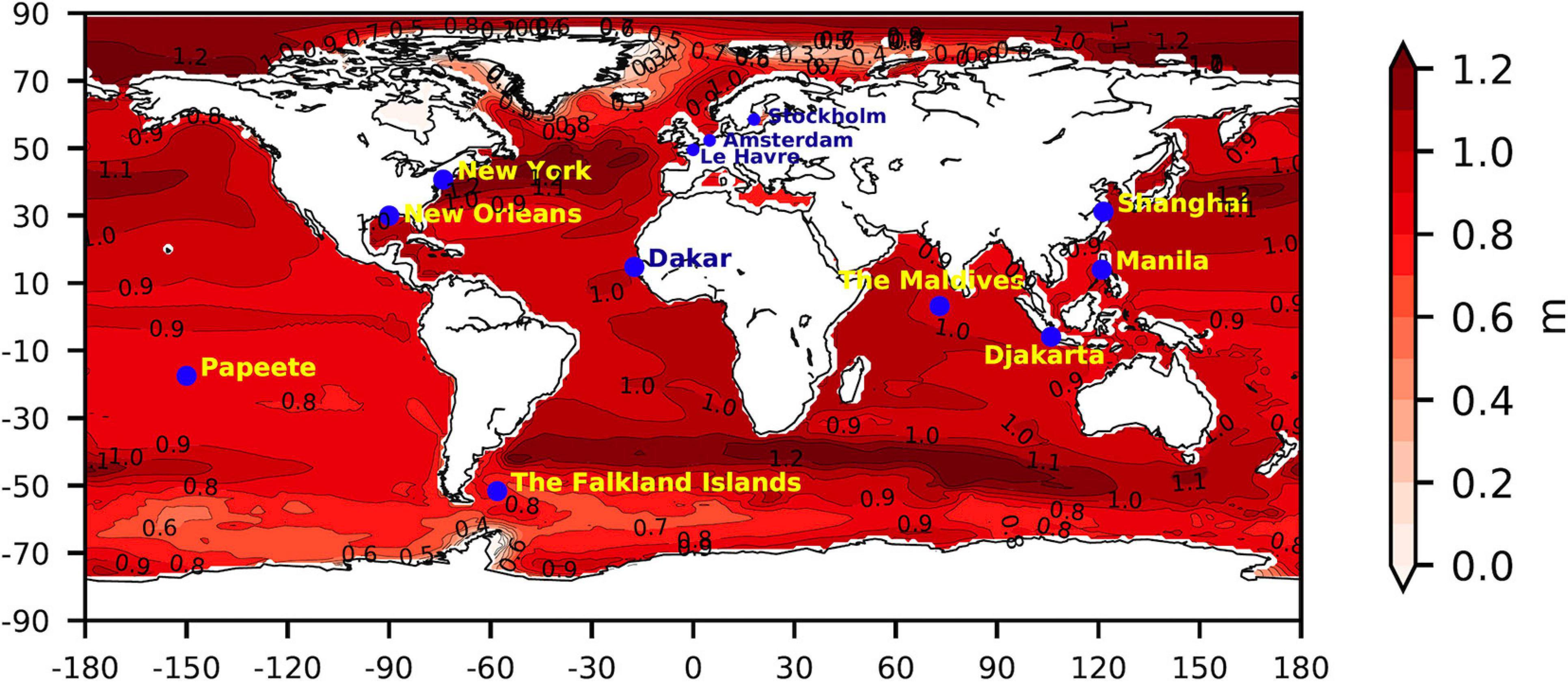
Figure 1. Regional sea-level change (m) in 2100 relative to 1986–2005 in RCP8.5. The selected sites for discussing regional scenarios are represented by the blue circles. Each value for each grid cell corresponds to the upper-end of the likely range obtained from sea-level projections provided by the Integrated Climate Data Center (Carson et al., 2016).
Method: Approach for Assessing HESs Change
General Approach
High-end sea-level scenarios are defined as unlikely (low probability), but possible, scenarios for future sea-level changes (Jevrejeva et al., 2014). Approaches to estimate HESs use various lines of evidence (Stammer et al., 2019). The most common approach is a probabilistic framework combining emission scenarios from the IPCC (RCPs) and estimates from simulation of the individual components of sea-level change based on a model selection and assumptions on ice-sheets contributions (Jevrejeva et al., 2019). However, relying on the highest quantiles of probabilistic sea-level projections is not always an appropriate method to estimate HESs, especially when the upper quantiles do not necessarily match the outcomes of processes not taken into account in the physical modeling of future sea-level changes. For example, relying on the upper quantiles of a distribution of the future Antarctic contribution to SLR assuming the marine ice-sheet instability (MISI) cannot quantitatively reflect the possibility of the marine ice-cliffs instabilities (MICI) (DeConto and Pollard, 2016; Kopp et al., 2017; Jevrejeva et al., 2019). In such cases of recognized ignorance, expert elicitation has been proposed as a way to overcome this difficulty (Bamber and Aspinall, 2013; B19).
Here, we use a combination of physical-based models and expert elicitation evidence, as illustrated in Figure 2. Our major goal is the regionalization of future sea-level changes as well as highlighting departure from GMSL for two emission scenarios and for three critical time horizons. We combine the projections for sterodynamic, glaciers, GIA and land water storage (LWS) from physical-based models with the future GrIS and AIS contributions from the last updated expert elicitation estimates of B19. Our projections are high-end because we consider the upper quantiles of these physical-based models or expert elicitations. Hence, the selection of expert-elicitation or physical models is guided by our motivation to select high-end scenario. Specifically, we distinguish two cases:
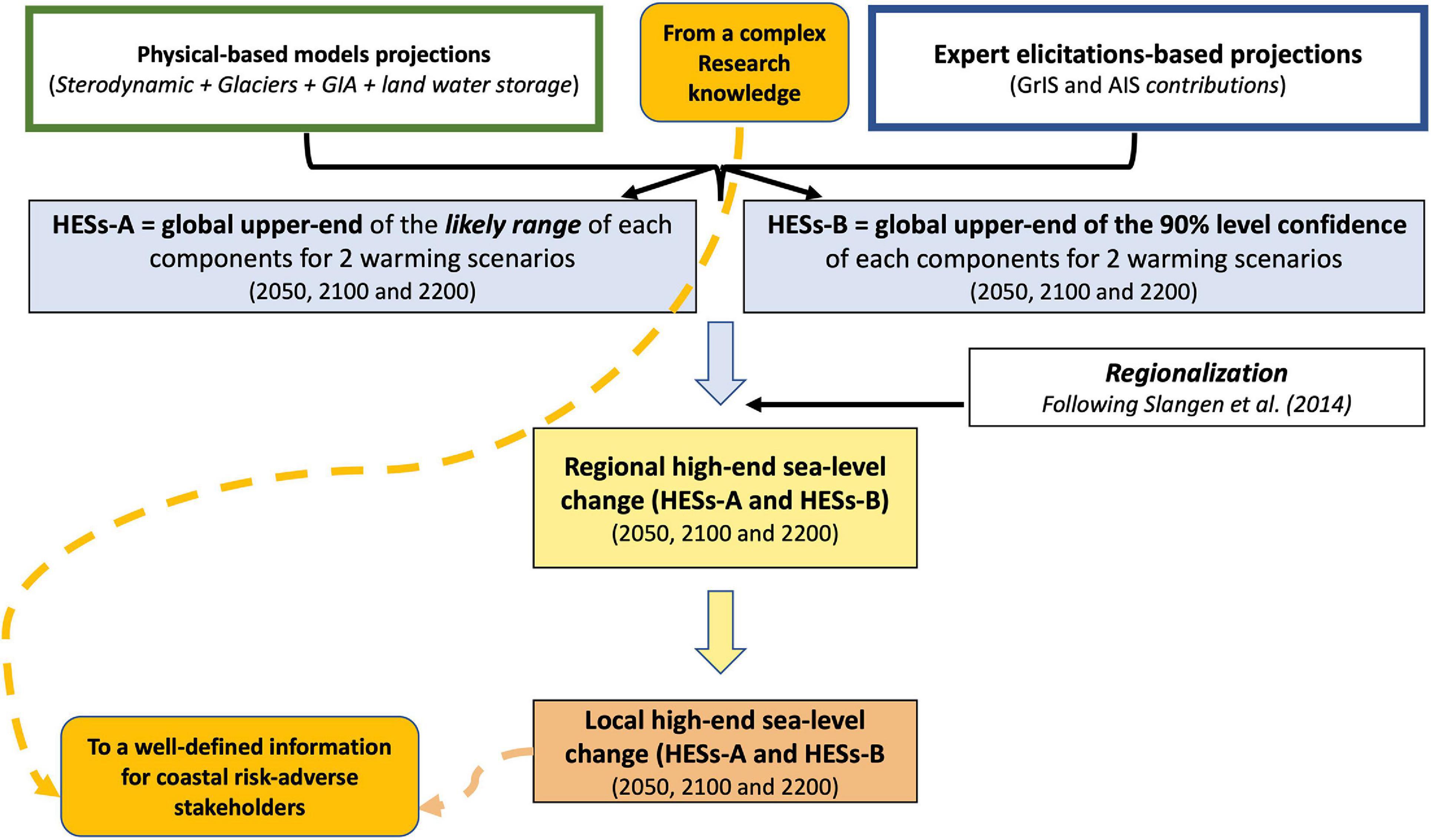
Figure 2. Scheme of our general approach for assessing global to regional and local HESs. Blue boxes display high-end design choices that can be adjusted depending on user’s preferences.
- if is no specific reason to consider a high-end well above the projected contribution (e.g., sterodynamic or glacier components), we rely on the high quantiles of the distribution (83rd and 95th percentiles).
- if some experts consider that high ends well above the projected contribution can be possible (e.g., Antarctica and Greenland ice melting), we consider the higher quantiles of an authoritative structured expert-elicitation of future ice-sheets melting to SLR.
The structured expert judgment estimate of B19 has the advantage to introduce non-Gaussian uncertainty into the tails of GrIS and AIS contributions, taking into account physical processes that are not necessarily represented by all ice-sheet models. We construct HESs for the two emissions scenarios from B19, the low emission scenario slightly warmer than RCP2.6 from IPCC AR5 and the high emission scenario almost as warm as RCP8.5 from IPCC AR5. We assume the low and high emission scenarios to be the same as RCP2.6 and RCP8.5 scenarios with regard to glaciers and sterodynamic contributions to global sea-level change. B19 do not account for the large temperature uncertainty from each RCP, and they assume temperature stabilization at 5°C for their high scenario, which can be considered optimistic in terms of climate forcing (Collins et al., 2013). Yet, their ice-sheets melting projections belong to the highest in the published literature, and can therefore be considered high-end.
We first build two HESs for GMSL combining each sea-level change contribution: HESs-A based on the upper-end of the likely range (83rd percentile) and HESs-B based on the upper-end of the 90% confidence level (95th percentile) of the distribution estimates of the different components of sea-level change. We do not pretend that summing 95th(83rd) percentiles for each component results in 95th(83rd) percentile projection: this would be true only for fully correlated components. We just take these percentiles to derive a HESs scenario, without providing a probability associated to it, as in Jevrejeva et al. (2014). The probability of these scenarios is low, but it cannot be quantified because we do not know the dependencies between contributions (Le Bars, 2018).
We then regionalize HESs following the method of Slangen et al. (2014): we sum the regional sterodynamic term, the regional sea-level equivalent (SLE) change from barystatic-GRD using fingerprint, a constant geographical pattern which generates the spatial sea-level variability induced by the mass redistribution on the Earth (see Supplementary Material for more details), and the regional GIA-induced sea-level change. While fingerprints will evolve over time or for varying temperature, and also depending on the exact source of melting (Meyssignac et al., 2017), we assume that they do not change over time as a first approximate, following previous studies (Slangen et al., 2014).
Sterodynamic Component
We use the thermal expansion projections of Kopp et al. (2014). These projections are based on a subset of 29 CMIP5 GCMs and result in a larger thermal expansion than that provided by the 21 CMIP5 GCMs used for the IPCC AR5 (Church et al., 2013). Note that the 29 CMIP5 GCMs of Kopp et al. (2014) comprise all the 21 CMIP5 GCMs of the IPCC AR5. The thermal expansion projections of Kopp et al. (2014) have the advantage to extend until 2200. Yet, the number of sterodynamic CMIP5 model outcomes drops from 29 to 6 models between 2100 and 2200 for the RCP8.5 scenario and from 20 to 6 models for the RCP2.6 scenario (see details in Kopp et al., 2014). The substantial difference in the number of models leads to a small discontinuity and a variance reduction at the start of the 22nd century. We select two high-end scenarios: HESs-A corresponds to the upper-end of the multi-model likely range (83rd percentile) from Kopp et al. (2014), while HESs-B corresponds to the 95th percentile (see values in Table 1). Our estimates for the sterodynamic component are slightly higher than the 83rd percentile of SROCC projections (Oppenheimer et al., 2019), and therefore can be considered high-end.
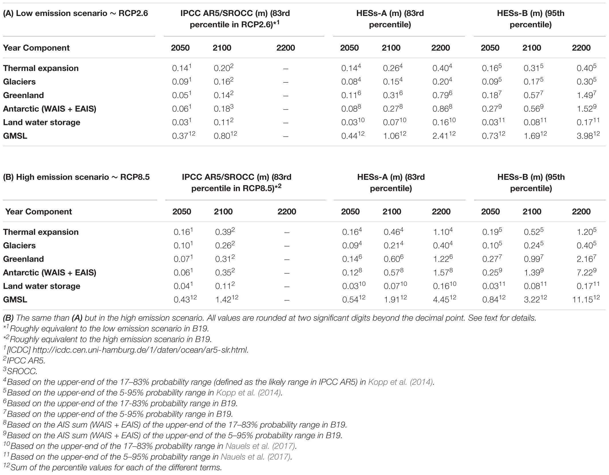
Table 1. (A) Global mean sea-level changes (m) in the low emission scenario by 2100 relative to the end of the 20th century of each sea-level contribution for (left) the IPCC AR5/SROCC upper-end of the likely range (83th percentile), (middle) HESs-A and (right) HESs-B.
To produce the regional SLR of the sterodynamic contribution, we use the spatial patterns of ocean dynamic sea-level changes of the IPCC AR5 models. This relies on the assumption that the regional variability of sea-level sterodynamic projections is driven by the same mechanisms in Kopp et al. (2014) and for the IPCC AR5, as suggested by Couldrey et al. (2021).
Only a subset of climate models deliver information in semi-enclosed seas, which leads to significant differences on both sides of the strait of Gibraltar (West-Atlantic and Mediterranean seas) and Danish Straits (North and Baltic seas), for example. Hence, to eliminate these potential sources of errors in HESs, we constrain the sterodynamic component within each semi-enclosed basin with that of the oceanic area, where all models are available, as in Thiéblemont et al. (2019). This approach is supported by studies analyzing the processes governing multi-decadal sea-level changes e.g., in the Baltic Sea (Weisse et al., 2019).
Barystatic-GRD Components
Glaciers
The glaciers projections are obtained combining process-based glacier models and output (precipitation and temperature) projections from CMIP5’s AOGCMs (Slangen and van de Wal, 2011). By 2100(2050), IPCC AR5 estimated an upper-end of the likely range of 0.16(0.1) m for RCP2.6 and 0.26(0.11) m for RCP8.5. Lower upper-end of the likely range projections were estimated by Marzeion et al. (2012) with 0.15 m from non-Antarctic glaciers by 2100 for RCP2.6 and 0.21 cm for RCP8.5. More recent modeling estimates by Huss and Hock (2015), also project slightly lower glacier mass losses than IPCC AR5 (Slangen et al., 2017). Given these slight differences in glacier mass loss projections between IPCC AR5 and updated studies, we opt for the Marzeion et al. (2012) projections by 2100, also used in Kopp et al. (2014) who provide in addition the projections of glaciers and GMSL for 2050 and 2200. Similarly to oceanographic process, GCM-based model projections of glacier contribution rely on a significantly reduced number of models after 2100 (Kopp et al., 2014). Here again, this limitation is considered by rounding 22nd century projections to the nearest decimeter. HESs-A for the glaciers contribution is defined using the upper-end of the multi-model likely range (83rd percentile) of Kopp et al. (2014), while HESs-B is defined as the upper-end of the 90% confidence level under normality hypothesis (95th percentile). Our glacier’s SLE estimates for each emission scenario, each HESs and each time horizon retained, are listed in Table 1. Because our estimates of the Glacier contribution to SLR are close to the 83rd percentile of SROCC projections (Oppenheimer et al., 2019), they can be considered as a realistic high-end. The regional SLR of the glaciers contribution is obtained from the fingerprint of glaciers sea-level changes used in IPCC AR5, and provided by the Integrated Climate Data Center (ICDC) of Hamburg University (Carson et al., 2016).
Ice-Sheets
GrIS and AIS are the planet’s ice-sheets and contain more than 65% of the Earth’s freshwater (Church et al., 2013). AIS is larger than GrIS and contains about eight times more ice than the latter, corresponding to 58.2 against 7.3 m SLE (Church et al., 2013). Considering a complete melting of both ice-sheets, GMSL would rise by roughly 65 m relative to present-day (Alley et al., 2005). While such a dramatic global SLR is excluded within the coming centuries (Pfeffer et al., 2008), both ice-sheets are losing mass, increasingly faster (Rignot et al., 2011; Shepherd et al., 2018). By 2100 and beyond, ice-sheets will continue to melt, even with strong mitigation measures to maintain global warming under 2°C relative to preindustrial global temperatures. Sea-level change driven by mass transfer from ice-sheets melting to the ocean can be explained through two physical processes which are the surface mass balance (SMB) and the dynamic effect (DYN). The former corresponds to the sum of accumulation and ablation driven by atmospheric processes and is quite well understood, while the latter is driven by changes in the dynamical discharge of glaciers and marine ice-sheets.
IPCC AR5 estimated that by 2100 the upper-end of the likely range of GrIS’s melting would be 0.28(0.01) m under RCP8.5(2.6) scenario, controlled by SMB by roughly two thirds. Since IPCC AR5, GrIS contribution to sea-level change has been slightly reevaluated (Fürst et al., 2015; Vizcaino et al., 2015), generally suggesting future Greenland ice dynamic losses are self-limited, although potentially substantial in marine terminating glaciers of west Greenland (Choi et al., 2021). SROCC estimates of GrIS’s contribution to future sea-level are the same as those reported in IPCC AR5.
The AIS contribution to sea-level change is broadly and vigorously debated in the literature (SROCC). The associated uncertainties are the largest and strongly depend on the understanding of DYN processes which trigger ice-sheet mass loss and their evolution under global warming. The two mechanisms involved are MISI, probably underway in West-Antarctica (Joughin et al., 2014; Rignot et al., 2014), and MICI, which has not been observed in Antarctica in the modern era, and whose contribution to past sea-level changes during previous interglacial is debated. It is unsure that MICI can be initiated during the 21st century (DeConto et al., 2019). Recently, SROCC reassessed upward the upper-end of the likely range of AIS contribution to GMSL: 0.37 m by 2100 under RCP8.5, against the 0.19 m provided by IPCC AR5, but this does not include a potential onset of MICI. Yet, if MICI is initiated during the 21st century, the ice-sheet of Antarctica may contribute by 0.8 (Edwards et al., 2019) or 1 m (DeConto and Pollard, 2016) in 2100, well above the projections of SROCC.
Here, we use the most recent elicitations-based projections of B19 on ice-sheet contributions, which give an upper-end of the likely range at 0.31(0.60) m by 2100 for the low(high) emission scenario. B19 report that their results have probably been influenced by expert reflecting the following research results: (1) paleo-evidences showing the sensitivity of the Antarctic ice-sheet to CO2 changes during past interglacial; (2) recent results of MICI (3) the warming trends in arctic and increasing contribution of Greenland to SLR since two decades, which experts have assumed being a consequence of external forcing in the B19 study. As a consequence, the uncertainties of B19 projections are revised upwards compared to Bamber and Aspinall (2013). HESs-A for the ice-sheets melting contribution is defined using the upper-end of the likely range (83rd percentile) from B19, while HESs-B is defined as the upper-end of the 90% confidence level under normality hypothesis (95th percentile) (Table 1). As noted in section “General approach,” the temperature assumptions in B19 are optimistic in the sense that they assume a stabilization at 5°C after 2100. Yet, Table 1 shows that their 95th percentile reaches 1.39 m for 2100, which is comparable to the results of DeConto and Pollard (2016) for RCP8.5 (1.14 ± 0.36 m). Hence, the B19 scenarios can be considered high-end.
B19 provided the total GIS contribution and separated the West Antarctic ice-sheet (WAIS) contribution from that of the East Antarctic ice-sheet. In IPCC AR5, the regional SLR of the ice-sheet contributions is obtained using the fingerprint of ice-sheet sea-level changes, using a separate fingerprint for the DYN effects and for the SMB effects. Here, we compute SLR of the ice-sheet contributions using both fingerprints used in IPCC AR5 for both ice sheets, thus assuming that melting is not uniform on the ice-sheet but that melting will be more prominent in West Antarctica and West Greenland. Specifically, we assign a weight of 0.33 to the fingerprint centered on West-Greenland and above 0.75 to the fingerprint centered on West-Antarctica (precise value for West-Antarctica, as in B19). Different assumptions on the precise location of melting would result in large differences in sea-level change scenarios close to the ice-sheet, but small differences far from it, where most people live.
Land Water Storage (LWS)
This contribution to SLR is driven by two major processes: the water impoundment, which contributes to mitigate SLR, and groundwater depletion which increases SLR. Projected anthropogenic LWS contribution to SLR and associated uncertainties are under debate due to incomplete process understanding (Konikow, 2011; Pokhrel et al., 2012; Wada et al., 2012, 2016; Church et al., 2013; Frederikse et al., 2020). Since the late 20th century, water storage contribution has decreased (Gregory et al., 2013), embodying groundwater depletion as the main anthropogenic LWS contribution to SLR over the 21st century and beyond. Since the IPCC AR5 projections which considered a 0.11 m SLR due to groundwater overuse, Wada et al. (2016) revised estimates assessing that previous studies overestimated groundwater depletion contribution to SLR without considering that only ∼80% of annually depleted groundwater ends up in the oceans, reducing the Wada et al. (2012) SLR contribution estimates from groundwater depletion by 20%.
We use the LWS projections of Nauels et al. (2017). These projections are based on the approach used by Wada et al. (2012), corrected by the 20% fraction of depleted groundwater that does not end up in the global ocean (Wada et al., 2016), adding extended projections up to 2200 considering the 30-year average annual depletion rate for the period 2071–2100. To do so, Nauels et al. (2017) assumed that human water use and groundwater extraction will carry on beyond 2100.
As in previous studies, we assume that LWS contribution to SLR is climate emission scenario-independent as differences are insignificant by the end of the 21st century, uncertainties are large together and processes at play beyond 2100 are underdetermined (Church et al., 2013). Our LWS’ SLE estimates for each HESs and time horizon are listed in Table 1. They are comparable to the 83rd percentile in SROCC projections, and can therefore be considered high-end. The regional SLR of the LWS contribution is obtained from the fingerprint of LWS sea-level changes used in IPCC AR5, and provided by ICDC.
Glacial Isostatic Adjustment (GIA)
Within IPCC AR5, GIA uncertainties are taken into account using two different GIA models (Church et al., 2013), whereby the best estimate is the mean of the two models and “one standard error of the GIA uncertainty is evaluated as the departures of the two different GIA estimates (from ICE-5G and ANU/SELEN models) from their mean value” (Church et al., 2013). Here, the GIA-induced regional sea-level change is defined for the HESs-A as the 1∗standard deviation around the mean, and for the HESs-B as 1.7∗regional standard deviation around the mean (i.e., upper-end of the 90% confidence level under normality hypothesis). GIA projections for the 22nd century are obtained by linearly extrapolating the 21st century values.
Results
This section presents our resulting HESs as a function of emission scenarios and time horizons (Tables 2, 3 and Figure 3). Supplementary Figure 3 allow to illustrate more precisely global patterns relative to GMSL.
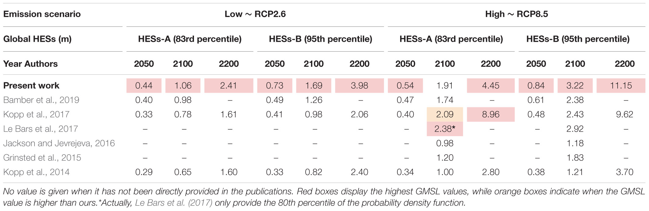
Table 2. Global HESs (m) as provided in selected recent publications and in the present work.
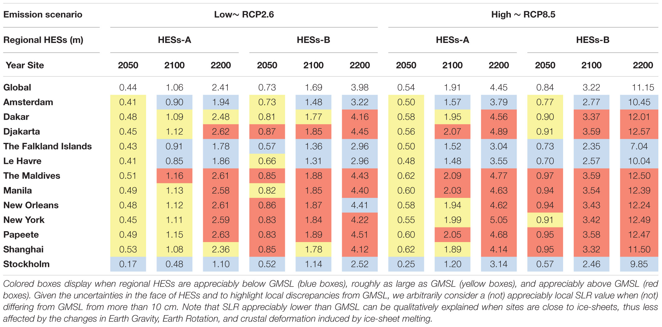
Table 3. Regional HESs (m) for the selected sites given by HESs-A and HESs-B for each emission scenario and for each time horizons (2050, 2100, and 2200).
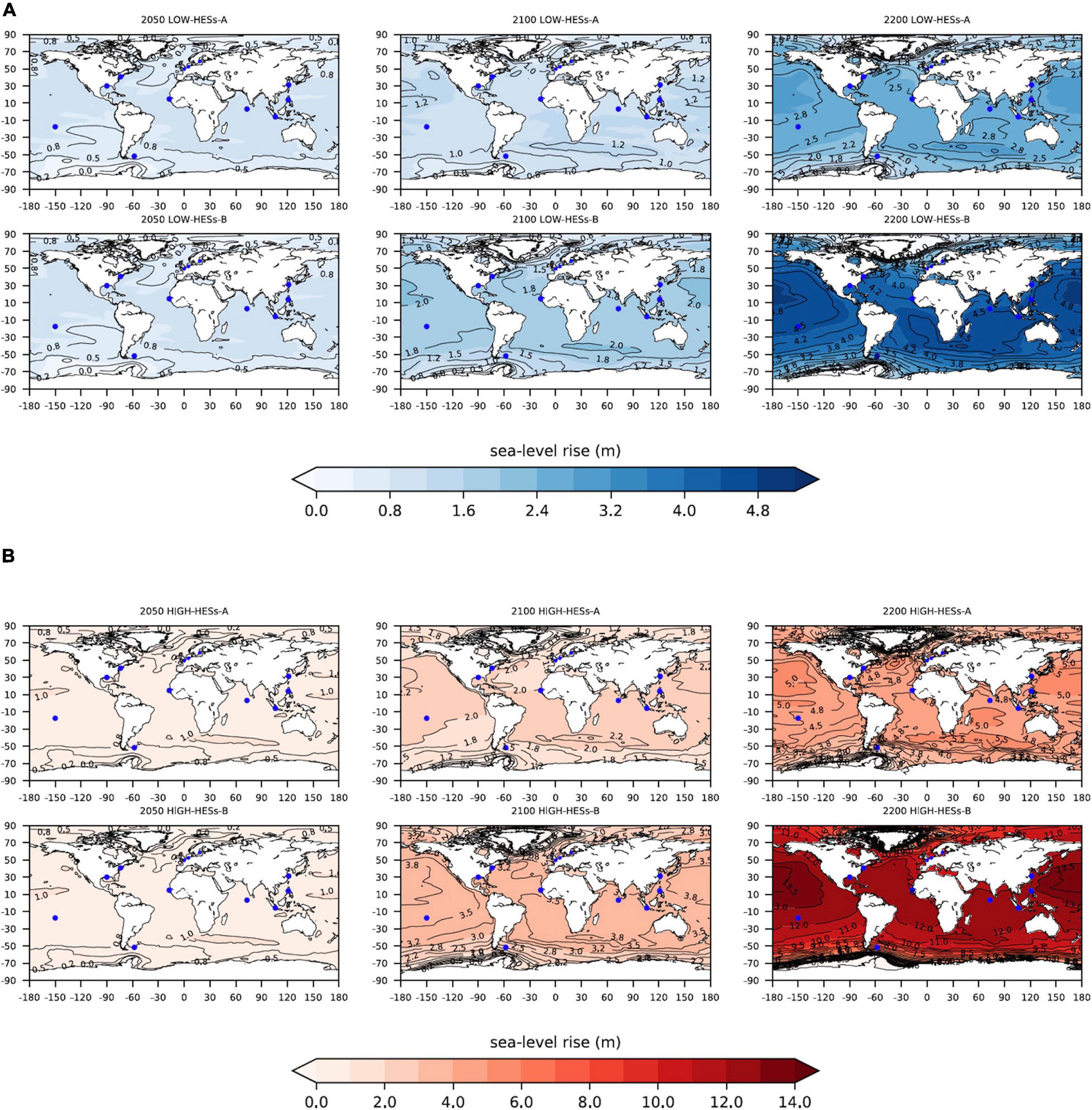
Figure 3. HESs at global scale for (first row) HESs-A and (second row) HESs-B in (A) the low emission scenario and (B) the high emission scenario. Colors and contours display SLR (m) by (left) 2050, (middle) 2100, and (right) 2200 relative to 1986–2005. Blue circles represent the selected sites (refer to Figure 1 for the names) discussing from regional to local HESs.
Global HESs
Under the low and high emission scenarios, both global HESs-A and HESs-B are larger than most of the values discussed in recent publications providing global HESs, regardless of the time horizon (Table 2). Although our global HESs estimates are built upon the same evidence as B19, they are substantially larger. This is because these authors assume dependencies between the various processes, so that the total ice-sheet contribution is not simply the sum of each ice-sheet contribution. Here, in contrast to the approach of B19, we explore global HESs that are not associated with any precise probability.
In 2050, HESs-A provides a GMSL roughly the same as B19 for both, low and high, emission scenarios, while HESs-B projects a 0.73(0.84) GMSL in the low(high) emission scenario, that is approximately 25% larger than B19. In 2100, for HESs-A, in the low(high) emission scenario, we found HESs values for GMSL that reach 1.06(1.91) m that is approximately 10% larger than in B19, while for HESs-B GMSL may increase up to 1.69(3.22) m that is approximately 25% larger than in B19. However, in the high emission scenario Kopp et al. (2017) and Le Bars et al. (2017) found a higher global HESs than our HESs-A. In fact, these two studies both included MICI from DeConto and Pollard (2016), that is, the largest GrIS and AIS melting projected so far by means of ice-sheet melting modeling. Hence, while the 1.69 m GMSL suggests that HESs could be relevant even for low emission scenarios, the 3.22 m GMSL is consistent with studies assuming possible rapid melting processes induced by MICI (DeConto and Pollard, 2016) that could cause a GMSL rise exceeding 1 m by 2100 (SROCC). Our results are slightly higher than those of Jevrejeva et al. (2014), who used a similar method: this is because we use different assumptions for the thermal expansion and glacier contributions, and also because their study relied on the previous expert elicitation from Bamber and Aspinall (2013). In 2200, GMSL may increase up to 2.41(4.45) m for HESs-A and 3.98(11.15) m for HESs-B in the low(high) emission scenario. These values are far larger than SROCC projections by the end of the 22nd century. They are also substantially larger than the SLR projections of Kopp et al. (2014), whose highest quantiles were constrained by the previous expert elicitation conducted by Bamber and Aspinall (2013). However, in the high emission scenario Le Bars et al. (2017) found a higher global HESs than our HESs-A, as they include MICI from DeConto and Pollard (2016).
From Global to Regional HESs
In this sub-section, we describe the spatial divergence of HESs and the regional contributions to HESs for two large areas (the northern Atlantic, Figure 4, and the south-eastern Pacific, Figure 5), as they show both important sea-level change gradients and host highly inhabited coastal cities, lands and islands (e.g., Amsterdam, Dakar, Le Havre, New Orleans, New York, Papeete, and Stockholm). While the coastal areas around the Indian Ocean, the north-eastern Pacific and the western Pacific also host inhabited coasts and islands, we choose not to describe them as they show a more homogeneous sea-level change pattern (see Figure 3 which displays sea-level spatial distribution at global scale). As the patterns for both emission scenarios are fairly similar (with lower values in the low emission scenario, see Figure 3A), we only discuss HESs spatial distribution in the high emission scenario. Supplementary Figures 1, 2 allow to illustrate more precisely regional patterns relative to GMSL.
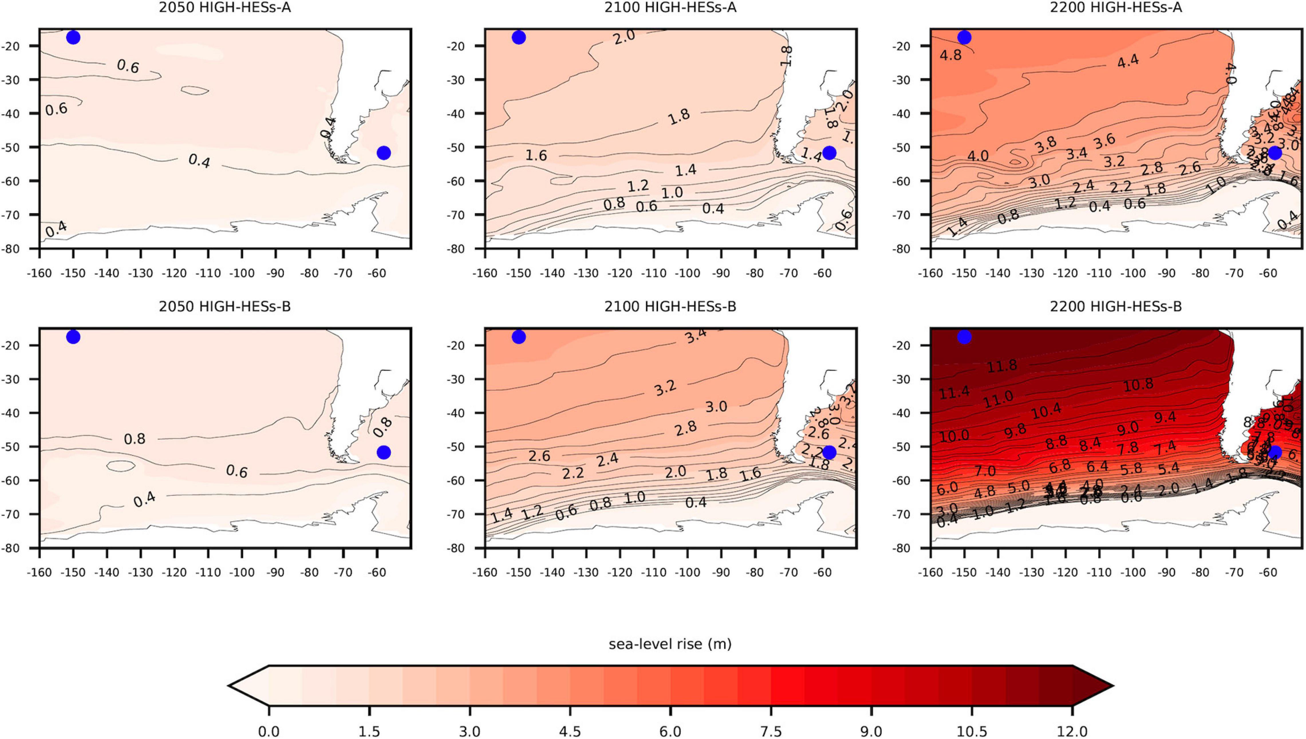
Figure 4. Regional HESs for (first row) HESs-A and (second row) HESs-B in the northern Atlantic. Colors and contours display SLR (m) by (left) 2050, (middle) 2100, and (right) 2200 relative to 1986–2005. Blue circles represent the selected sites (refer to Figure 1 for the names) discussing from regional to local HESs.
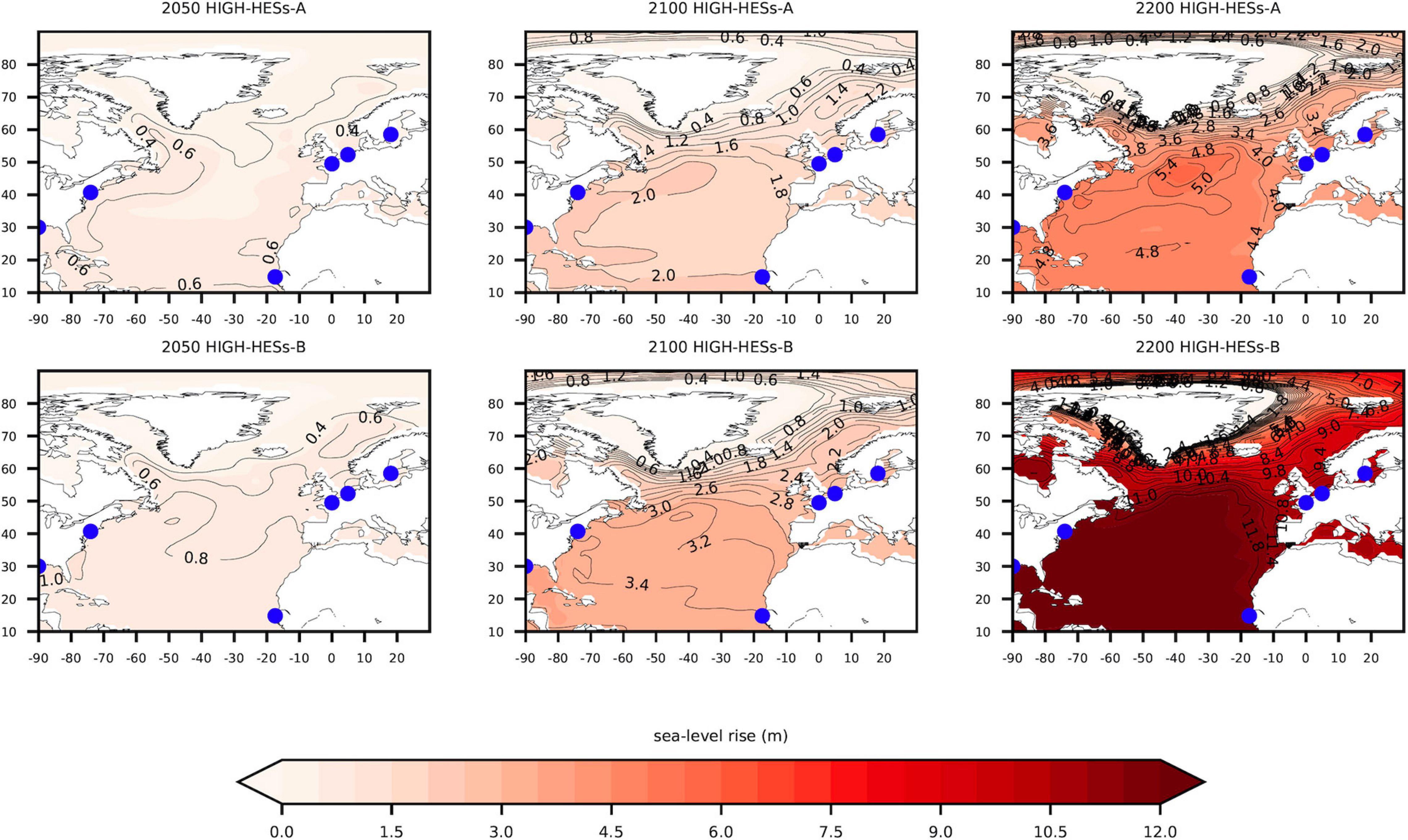
Figure 5. The same as Figure 4, but in the south-eastern Pacific.
As time goes by and as HESs get worse, the northern Atlantic(south-eastern Pacific) displays an increasingly important southwest-northeast(south-north) sea-level change gradient (Figures 4, 5). Both regions show increasing rates of minimum(maximum) SLR at high(low-to-mid) latitudes, close to (far from) ice-sheets, resulting from the redistribution of ice mass from land to ocean. As a consequence, HESs values are substantially lower than GMSL in the vicinity of ice-sheets, regardless of time horizon. This is an obvious consequence of the gravitational effects associated to ice-sheet mass losses (Spada et al., 2013), which are larger here than in previous studies due to the more substantial amount of mass losses in ice-sheets involved by high-end scenarios. Hence, HESs display spatial variability mostly due to the sterodynamic contribution, ice-sheets melting and the GIA effects (Slangen et al., 2014). Here, we detail the role of each sea-level contribution.
High-end sea-level scenarios patterns in the northern Atlantic result from several main processes (Figure 4). First, the sterodynamic component through the combination of the northward shift of the North Atlantic Current (Landerer et al., 2007) and a weakening of the meridional overturning circulation (Yin et al., 2009), increasing SLR particularly on the northeast coast of the United States. Second, the ice-sheets contributions, decreasing(increasing) SLR close to (far from) ice-sheets, and the GIA contribution acting on vertical ground motions in regions where large ice-sheets existed during the LGM. While in Scandinavia GIA induces high rates of uplift, the region of the Chesapeake Bay in the East-US coast undergoes substantial subsidence. As a consequence, as time passes by and HESs worsen, SLR in the northeast coast of the United States might be not only larger than GMSL, but also higher than SLR along other northern Atlantic coasts, such as the European and east African coasts. SLR in northern Europe (e.g., around the Gulf of Finland) is lower due to the effects of GIA (Figure 4). Over the Arctic, HESs show higher SLR values (Figure 4).
As to the south-eastern Pacific, Slangen et al. (2014) described the south-north sea-level change gradient – a meridional gradient across the Antarctic Circumpolar Current – as the result of several main processes. First, the combination of low thermal expansion coefficients regarding colder temperatures in the extreme south and a strengthening and southward shift of the Antarctic Circumpolar Current in response to increasing CO2 emissions. Second, the West AIS dynamic, which leads to drastic SLR gradients from south to north in the South America continent (Figure 5). As a consequence, in 2100 and for HESs-B, for example, at the southern tip of Chili SLR might be lower by more than 1 m than the 3.22 GMSL, whereas in northern Chili SLR might equal GMSL (Figure 5). Yet, the actual values in this region are dependent on the location of melting in the Antarctic ice-sheet, an uncertainty which is not accounted for in this study.
From Regional to Coastal City and Island Scale HESs
For each coastal city and island scale HESs, time horizon and emission scenario, the reader can refer to both Figure 3 displaying sea-level spatial distribution at global scale and Table 3. Given the uncertainties in HESs and to highlight local departure from GMSL, we arbitrarily consider that the difference between local SLR and GMSL is not appreciable when it differs by less than ±10 cm. For example, SLR is appreciably lower than GMSL close to ice-sheets.
2050
In 2050, for HESs-A in the low/high emission scenario, SLR does not appreciably differ from GMSL (low emission scenario: 0.44/high emission scenario: 0.54 m) in Amsterdam (0.41/0.50 m), Dakar (0.48/0.58 m), Djakarta (0.45/0.56 m), the Falkland Islands (0.43/0.50 m), Le Havre (0.41/0.48 m), the Maldives (0.51/0.62 m), Manila (0.49/0.60 m), New Orleans (0.48/0.58 m), New York (0.45/0.55 m), Papeete (0.49/0.60 m), and Shanghai (0.53/0.62 m), while it may be appreciably lower than GMSL for both emission scenarios in Stockholm due to GIA (0.17/0.25 m). For HESs-B in the low emission scenario, SLR appreciably differ from GMSL (0.73 m) in the Falkland Islands (0.57 m) and Stockholm (0.52 m) where it is appreciably below GMSL. In Djakarta (0.87), the Maldives (0.85 m), New Orleans (0.86 m), New York (0.83 m), Papeete (0.83 m), and Shanghai (0.85 m) it appreciably exceeds GMSL. For HESs-B in the high emission scenario, SLR does not appreciably differ from GMSL (0.84 m) in Amsterdam (0.77 m), Dakar (0.90 m), Djakarta (0.91 m), and New York (0.91 m), whereas it may be appreciably higher than GMSL in the Maldives (0.97 m), Manila (0.94 m), New Orleans (0.94 m), Papeete (0.95 m), and Shanghai (0.95 m) and lower than GMSL in the Falkland Islands (0.73 m), Le Havre (0.70 m), and Stockholm (0.57 m). This result illustrates that provided there is no additional vertical ground motion besides GIA, 2050 is a relevant time horizon for local coastal stakeholders to start considering regional sea-level projections in their adaptation plans.
2100
For HESs-A in the low emission scenario, SLR may appreciably differ from GMSL (1.06 m) in Amsterdam (0.90 m), the Falkland Islands (0.91), Le Havre (0.85 m), and Stockholm (0.48 m). It may appreciably differ from GMSL (1.91 m) in the high scenario not only in the latter four sites but also in Djakarta (2.07 m), the Maldives (2.09 m), Manila (2.03 m), and Papeete (2.05 m).
For HESs-B in the low emission scenario and relative to HESs-A, discrepancies increase with SLR appreciably differing from GMSL (1.69 m). These discrepancies include Djakarta (1.85 m), the Maldives (1.88 m), Manila (1.85 m), New Orleans (1.87 m), New York (1.84 m), and Papeete (1.89 m). For HESs-B in the high emission scenario, all the sites may appreciably exceed (Dakar, Djakarta, The Maldives, Manila, New Orleans, New York, Papeete, and Shanghai) or be lower (Amsterdam, The Falkland Islands, Le Havre, and Stockholm) than GMSL (3.22 m).
2200
For HESs-A in the low/high emission scenario, while SLR remains appreciably lower than the GMSL (2.41/4.45 m) in Amsterdam (1.94/3.79 m), the Falkland Islands (1.78/3.04 m), Le Havre (1.86/3.55 m), and Stockholm (1.10/3.14 m), it may appreciably exceed GMSL in Dakar (only in the high emission scenario, 4.56 m), Djakarta (2.62/4.89 m), the Maldives (2.61/4.77 m), Manila (2.58/4.63 m), New Orleans (2.61/4.62 m), New York (2.59/5.05 m), and Papeete (2.63/4.68 m). Regarding Shanghai, scenarios are not appreciably lower than GMSL in the low emission scenario and appreciably lower than GMSL in the high emission scenario.
For HESs-B in the low/high emission scenario, GMSL may reach 3.98/11.15 m and SLR may appreciably differ in all locations. Values are higher than GMSL in Dakar (4.16/12.01 m), Djakarta (4.45/12.57 m), the Maldives (4.43/12.50 m), Manila (4.40/12.39 m), New Orleans (4.41/12.24 m), New York (4.22/12.49 m), Papeete (4.51/12.47 m), and Shanghai (4.14/11.50 m). They are lower in Amsterdam (3.22/10.45 m), in the Falkland Islands (2.96/7.04 m), Le Havre (2.96/10.04 m), and Stockholm (2.52/9.85 m).
Regional Contributions to Coastal City and Island HESs
Figures 6A,B illustrate the different contributions to HESs for each site by 2050, 2100, and 2200 relative to 1986–2005.
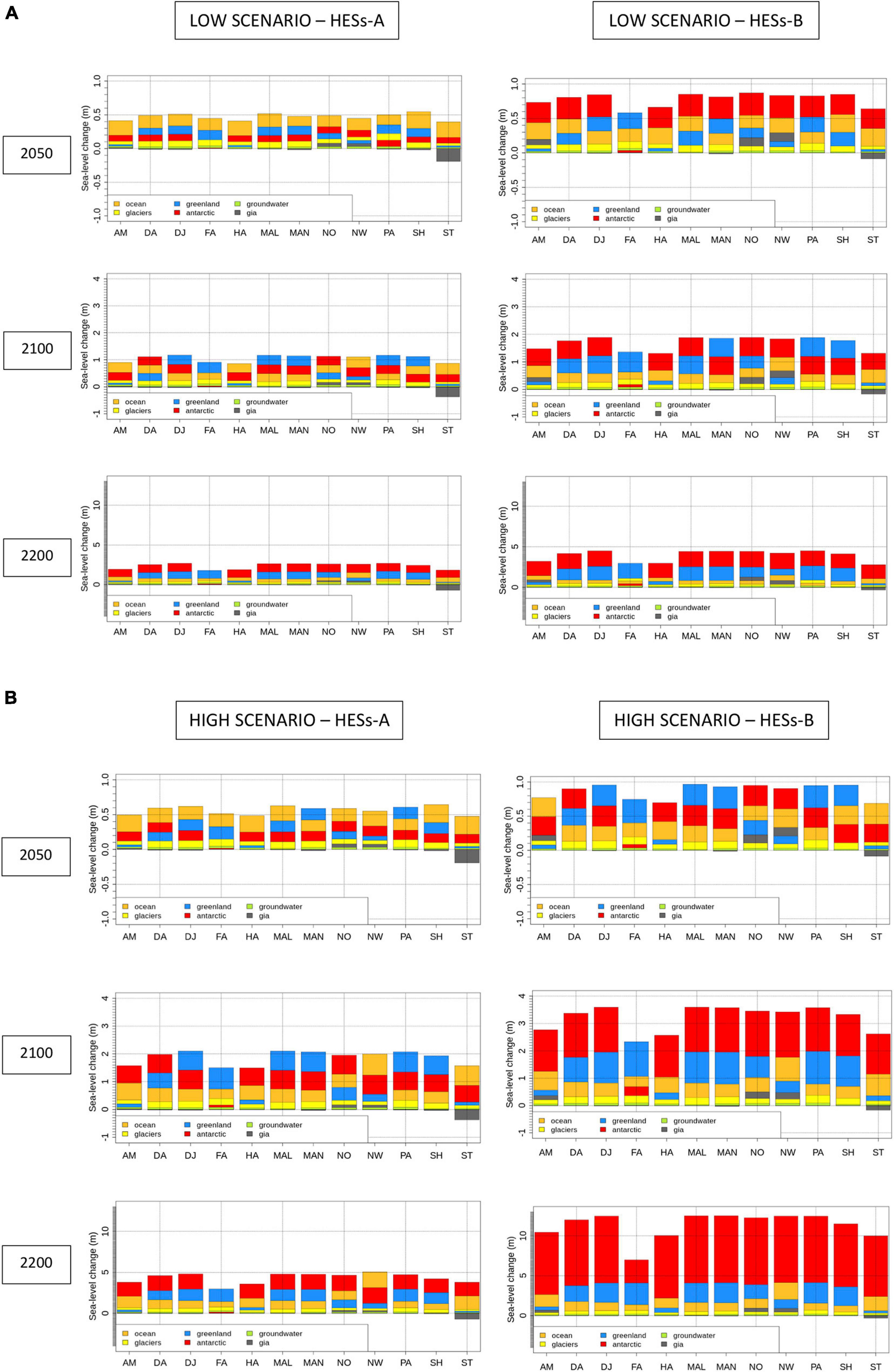
Figure 6. Contributions to sea-level change (m) by 2050, 2100, and 2200 relative to 1986–2005 for both HESs in (A) the low emission scenario at left(right) and (B) the high emission scenario. The X-axis indicates the twelve selected sites: AM (AMsterdam), DA (DAkar), DJ (DJakarta), FA (The FAlkland Islands), HA (Le HAvre), MAL (The MALdives), MAN (MANila), NO (New Orleans), NW (New York), PA (PApeete), SH (SHanghai), and ST (STockholm). The top of each bar of the histogram indicates the regional SLR for each site including all the contributions (see Table 3 for detailed values), while each color bar indicates the relative contribution to sea-level change for each component and are sorted in ascending order. Note that the boundaries of the Y-axis are different for each time horizon.
In 2100, for HESs-A and in the low emission scenario the largest contribution to sea-level changes are caused by sterodynamic oceanic processes in Amsterdam, Le Havre, New York, and Stockholm and are dominated by ice-sheets processes in the others cities. In the high emission scenario, ice-sheets processes seem to step up and dominate sea-level changes everywhere except in New York and Stockholm. In the high emissions scenario, the relative contribution of glaciers to SLR is more substantial than in the low emission scenario in all sites. Land water storage and GIA contribute to a lesser extent to SLR in all sites, except in Stockholm where GIA influences sea-level change almost at the same rate as oceanic or ice-sheets processes.
In 2200, for HESs-A in both emission scenarios, sea-level change would be driven mostly by ice-sheets, and then by sterodynamic oceanic processes in most of the twelve sites, except in Stockholm where GIA tends to dominate oceanic processes and substantially decrease SLR. Glaciers are the fourth contribution to SLR, except in New Orleans and New-York where GIA increases sea-level at least equally as important as Glaciers.
Discussion
Limitations
A number of limitations need to be remembered: first, the whole discussion on HESs comes from limited understanding of ice-sheet melting processes (Stammer et al., 2019). However, there is not a consensus in the community of ice-sheet glaciologists that such large contributions to SLR are physically plausible, as illustrated by the discussion around the MICI (DeConto and Pollard, 2016; Edwards et al., 2019). Another difficulty lies in the projections beyond 2100, which have less confidence than those applicable during the 21st century due to the lack of knowledge about GHG emissions.
Some of the choices made for designing our high-end scenarios can be revised to fit user preference. In particular, we selected two quantile levels (83th and 95th) to reflect different degrees of risk aversion (Hinkel et al., 2019; Thiéblemont et al., 2019), but others may be more relevant. As a caveat, the selection of a particular quantile level should be made with attention to the number of samples used to fit the probability distribution (Wilks, 1941). In other words, there is generally not enough information in probabilistic projections of sea-level contributions to realistically evaluate the 99th percentile level. Finally, even if we have updated the ice sheet-related sea level projections from B19, we note that we rely on a single probabilistic projection, which is not sufficient (Jevrejeva et al., 2019). One way forward to go beyond the limits of this study would be to “involve users with sea level information providers to co-design appropriate projections,” as promoted in projects aiming at developing climate services such as the ERA4CS.
Other Drivers of Change
A number of bio-physical and human processes have been overlooked in this study. For example, coastal hydrodynamic processes may alter our HESs by up to a few percent (e.g., Zhang et al., 2004, 2017). This can be considered negligible given the uncertainties surrounding HESs. More importantly, vertical ground motions such as subsidence or uplift (Nicholls et al., 2021), coastal sediment losses and accumulation (Toimil et al., 2020), potential changes in extreme water levels due to potential storminess, bathymetry or river flow changes, or human adaptation actions (Oppenheimer et al., 2019), may locally cause changes in flooding and erosion risks that are larger than the impacts of the HESs presented above. For example, while these HESs appear extremely high, especially by 2050 for high emissions, we recall that subsidence can generate similar relative sea-level changes: in some coastal areas of Manilla, groundwater extractions are causing subsidence in the order of 5 cm/year in the north-western coast of the city and 1 cm/year at the tide gauge close to the city center (Raucoules et al., 2013). While these processes are highly non-linear in time, they mean that locally, relative sea-level changes comparable to those found here in our worst case HESs can happen within 10 years. Similar issues are known to already happening in other rapidly developing cities, especially in Southeast Asia, such as Djakarta. However, the example of Shanghai (Wang et al., 2012) shows that reducing groundwater extractions or refilling aquifers can mitigate the phenomenon.
Relevance to Coastal Adaptation
This study can be considered as a step forward compared to the previous approach consisting in defining high-end scenarios based on global SLR projections (Purvis et al., 2008; Nicholls et al., 2014; Le Cozannet et al., 2015; Rohmer et al., 2019). In fact, we explicitly account for the regional implications of the high-end ice-sheets melting scenarios that might cause SLR exceeding the IPPC likely range. Neglecting this effect leads to underestimating high-end sea-level changes in a number of places: for example, Figure 3 shows that SLR in 2100 for the high emission scenario and HESs-B exceeds the global mean sea-level (GMSL, 3.22 m) in Dakar, Djakarta, the Maldives, Manila, New Orleans, New York, Papeete, and Shanghai (see Table 3 for detailed values). While this phenomena can be qualitatively anticipated based on the fingerprints associated with ice-sheets melting, in particular, this study provides quantitative insight.
Recent works suggest that such HESs are particularly relevant for decision makers and risk-averse stakeholders to implement informed adaptation measures (Haasnoot et al., 2013; Ranger et al., 2013; Nicholls et al., 2014). In particular, risk-averse stakeholders are looking forward to information on high-end SLR tails of the distribution outside the specified IPPC likely range (Hinkel et al., 2015, 2019; Le Cozannet et al., 2017a). Hence, his study potentially brings relevant and context-specific SLR information to these risk-averse stakeholders (Hinkel et al., 2015, 2019; Stammer et al., 2019), but also to decision makers and any coastal end-users. One of the major results of our work is that the rate of SLR can differ substantially in different locations (see Figure 3 and Table 3). For example, in the high emission HESs-B scenario, the Maldives may experience a rise of sea-level that is comparable to the global mean until 2050. Then, SLR would accelerate substantially, so that sea-level may exceed GMSL by about 30 cm in 2100 due to GRD effects associated with mass losses in Antarctica and Greenland. This type of result can be relevant for adaptation practitioners considering the timing of adaptation (Haasnoot et al., 2020). Another important result of this study is the 1.69 m GMSL in 2100 for the HESs-B and in the low emission scenario (largely above the 0.59 m GMSL given by the upper-end of the likely range in SROCC), suggesting that HESs could be relevant even for low emission scenarios (see also Figure 3A).
Future research in this area may lead to excluding a number of scenarios that cannot be ruled out today. Meanwhile, risk-averse users concerned with long term decisions still need guidance (Hinkel et al., 2019), and may refer to the values presented in this paper and others (Nicholls et al., 2014; Thiéblemont et al., 2019). While these HESs are highly uncertain, they correspond to very high risk of economic, environmental and very likely human losses, and they deserve some attention in adaptation planning, as it has already made in several domains such as nuclear safety (Destercke and Chojnacki, 2008), food engineering (Baudrit et al., 2009), environmental risk (Baudrit et al., 2007), or CO2 geological storage-related risk (Loschetter et al., 2016).
Conclusion
This study delivers global and regional HESs. Such scenarios have a major societal relevance, because they induce either large adaptation needs, or they imply retreat of coastlines in highly vulnerable low-elevated lands and islands during the second half of the 21st century. Several studies delivered HESs using a probabilistic framework combining greenhouse gas emission scenarios and estimates from simulation of the individual components of sea-level change based on a model selection and assumptions on ice-sheets contributions. However, this is not always an appropriate method to estimate HESs, especially because the physical models of future sea-level changes do not take into account some non-linear dynamical ice-sheet processes. We have used published expert elicitation for ice-sheet contributions, combining physical-based model projections for glaciers, ocean sterodynamic effects and glacial isostatic adjustment, updated contributions from land-water. We highlight that provided there is no additional vertical ground motion besides GIA, the likely projected SLR might be significantly exceeded as soon as 2050. Today, planning and implementing coastal relocation, accommodation or protection typically takes several decades. Hence, our result means that for risk-averse coastal managers, adaptation decision horizons might be much closer than previously thought. Our results also suggest that HESs should be taken into account even for low emission scenarios.
The regional HESs presented in this paper can be used by risk-averse coastal stakeholders to determine adaptation pathways over the 21st century and beyond. However, local subsidence effects can still represent a substantial contribution to future relative sea-level changes in some areas such as Manila or Djakarta, and they need to be characterized where needed. By construction, HESs have a low probability to occur, but as their effects may be dramatic they cannot be excluded given the present state of knowledge. In the coming years, research on SLR and the ice-sheets evolution will precise the confidence that can be assigned to the different sets of HESs that are being considered today. This will allow coastal adaptation to progressively adjust their adaptation pathways to the level of effort that is required.
Data Availability Statement
The datasets presented in this study can be found in online repositories. The names of the repository/repositories and accession number(s) can be found below: https://vesg.ipsl.upmc.fr/thredds/catalog/IPSLFS/hdayan/Data_HESs/catalog.html.
Author Contributions
HD and GL conceived of the presented idea. HD performed the computations and carried out the analyses. All authors discussed the results and contributed to the final manuscript.
Funding
This study benefited from the IPSL Prodiguer-Ciclad facility is supported by CNRS, UPMC, Labex L-IPSL (Grant #ANR-10-LABX-0018), and the European FP7 IS-ENES2 project (Grant #312979). This study was supported by a grant from the French Ministry for an Ecological and Solidary Transition as part of the Convention on financial support for climate services and the ANR Storisk project (ANR-15-CE03-0003).
Conflict of Interest
The authors declare that the research was conducted in the absence of any commercial or financial relationships that could be construed as a potential conflict of interest.
Acknowledgments
We acknowledge the World Climate Research Programme’s Working Group on Coupled Modeling, which is in charge of the fifth Coupled Model Intercomparison Project, and we thank the climate modeling groups for producing and making available their model output. We acknowledge the Integrated Climate Data Center (ICDC, icdc.cen.uni-hamburg.de) University of Hamburg, Hamburg, Germany, for distributing the regional sea level data from IPCC AR5 as well as Kopp et al. (2014), Nauels et al. (2017), and Bamber et al. (2019) for making their data available.
Supplementary Material
The Supplementary Material for this article can be found online at: https://www.frontiersin.org/articles/10.3389/fmars.2021.569992/full#supplementary-material
Footnotes
- ^ https://www.aviso.altimetry.fr/en/data/products/ocean-indicators-products/mean-sea-level/products-and-images-selection-without-saral-old.html
References
Alley, R. B., Clark, P. U., Huybrechts, P., and Joughin, I. (2005). Ice-sheet and sea-level changes. Science 310, 456–460. doi: 10.1126/science.1114613
Bamber, J. L., and Aspinall, W. P. (2013). An expert judgement assessment of future sea level rise from the ice sheets. Nat. Clim. Chang 3, 424–427. doi: 10.1038/nclimate1778
Bamber, J. L., Oppenheimer, M., Kopp, R. E., Aspinall, W. P., and Cooke, R. M. (2019). Ice sheet contributions to future sea-level rise from structured expert judgment. Proc. Natl. Acad. Sci. U. S. A. 116, 11195–11200. doi: 10.1073/pnas.1817205116
Baudrit, C., Guyonnet, D., and Dubois, D. (2007). Joint propagation of variability and imprecision in assessing the risk of groundwater contamination. J. Contam. Hydrol. 93, 72–84. doi: 10.1016/j.jconhyd.2007.01.015
Baudrit, C., Hélias, A., and Perrot, N. (2009). Joint treatment of imprecision and variability in food engineering: application to cheese mass loss during ripening. J. Food Eng. 93, 284–292. doi: 10.1016/j.jfoodeng.2009.01.031
Carson, M., Köhl, A., Stammer, D., Slangen, A. B. A., Katsman, C. A., van de Wal, R. S. W., et al. (2016). Coastal sea level changes, observed and projected during the 20th and 21st century. Clim. Change 134, 269–281. doi: 10.1007/s10584-015-1520-1521
Choi, Y., Morlighem, M., Rignot, E., and Wood, M. (2021). Ice dynamics will remain a primary driver of greenland ice sheet mass loss over the next century. Commun. Earth Environ. 2:26. doi: 10.1038/s43247-021-00092-z
Church, J. A., Clark, P. U., Cazenave, A., Gregory, J. M., Jevrejeva, S., Levermann, A., et al. (2013). “Chapter 13: sea level change,” in Climate Change 2013: The Physical Science Basis. Contribution of Working Group I to the Fifth Assessment Report of the Intergovernmental Panel on Climate Change, eds T. F. Stocker, D. Qin, G.-K. Plattner, M. Tignor, S. K. Allen, and J. Boschung (Cambridge, NY: Cambridge University Press), doi: 10.1017/CB09781107415315.026
Collins, M., Knutti, R., Arblaster, J., Dufresne, J.-L., Fichefet, T., Friedlingstein, P., et al. (2013). “Long-term climate change: projections, commitments and irreversibility,” in Climate Change 2013 - The Physical Science Basis: Contribution of Working Group I to the Fifth Assessment Report of the Intergovernmental Panel on Climate Change, eds T. F. Stocker, D. Qin, G.-K. Plattner, M. M. B. Tignor, S. K. Allen, J. Boschung, et al. (Cambridge: Cambridge University Press).
Couldrey, M. P., Gregory, J. M., Oluwayemi, G., Griffies, S. M., Haak, H., Hu, A., et al. (2021). What causes the spread of model projections of ocean dynamic sea-level change in response to greenhouse gas forcing? Climate Dynam. 56, 155–187. doi: 10.1007/s00382-020-05471-4
Dangendorf, S., Hay, C., Calafat, F. M., Marcos, M., Piecuch, C. G., Berk, K., et al. (2019). Persistent acceleration in global sea-level rise since the 1960s. Nat. Clim. Chang 9, 705–710. doi: 10.1038/s41558-019-0531-538
DeConto, R. M., Ekaykin, A., Mackintosh, A., Van de Wal, R., Bassis, J., Cross-Chapter Box 8 | Future Sea Level Changes and Marine Ice Sheet Instability in Meredith, M., et al. (2019). “Polar regions,” in IPCC Special Report on the Ocean and Cryosphere in a Changing Climate, eds H.-O. Pörtner, D. C. Roberts, V. Masson-Delmotte, P. Zhai, M. Tignor, and E. Poloczanska (Geneva: IPCC).
DeConto, R. M., and Pollard, D. (2016). Contribution of Antarctica to past and future sea-level rise. Nature 531, 591–597. doi: 10.1038/nature17145
Destercke, S., and Chojnacki, E. (2008). Methods for the evaluation and synthesis of multiple sources of information applied to nuclear computer codes. Nucl. Eng. Des. 238, 2484–2493. doi: 10.1016/j.nucengdes.2008.02.003
Edwards, T. L., Brandon, M. A., Durand, G., Edwards, N. R., Golledge, N. R., Holden, P. B., et al. (2019). Revisiting Antarctic ice loss due to marine ice-cliff instability. Nature 566, 58–64. doi: 10.1038/s41586-019-0901-904
Frederikse, T., Landerer, F., Caron, L., Adhikari, S., Parkes, D., Humphrey, V. W., et al. (2020). The causes of sea-level rise since 1900. Nature 584, 393–397. doi: 10.1038/s41586-020-2591-2593
Fürst, J. J., Goelzer, H., and Huybrechts, P. (2015). Ice-dynamic projections of the Greenland ice sheet in response to atmospheric and oceanic warming. Cryosphere 9, 1039–1062. doi: 10.5194/tc-9-1039-2015
Gregory, J. M., Griffies, S. M., Hughes, C. W., Lowe, J. A., Church, J. A., Fukimori, I., et al. (2019). Concepts and terminology for sea level: mean, variability and change, both local and global. Surv. Geophys. 40, 1251–1289. doi: 10.1007/s10712-019-09525-z
Gregory, J. M., White, N. J., Church, J. A., Bierkens, M. F. P., Box, J. E., Van Den Broeke, M. R., et al. (2013). Twentieth-century global-mean sea level rise: is the whole greater than the sum of the parts? J. Clim. 26, 4476–4499. doi: 10.1175/JCLI-D-12-00319.1
Grinsted, A., Jevrejeva, S., Riva, R. E. M., and Dahl-Jensen, D. (2015). Sea level rise projections for Northern Europe under RCP8.5. Clim. Res. 64, 15–23. doi: 10.3354/cr01309
Haasnoot, M., Kwadijk, J., Van Alphen, J., Le Bars, D., Van Den Hurk, B., Diermanse, F., et al. (2020). Adaptation to uncertain sea-level rise; how uncertainty in Antarctic mass-loss impacts the coastal adaptation strategy of the Netherlands. Environ. Res. Lett. 15:034007. doi: 10.1088/1748-9326/ab666c
Haasnoot, M., Kwakkel, J. H., Walker, W. E., and ter Maat, J. (2013). Dynamic adaptive policy pathways: a method for crafting robust decisions for a deeply uncertain world. Glob. Environ. Chang 23, 485–498. doi: 10.1016/j.gloenvcha.2012.12.006
Hinkel, J., Church, J. A., Gregory, J. M., Lambert, E., Le Cozannet, G., Lowe, J., et al. (2019). Meeting user needs for sea level rise information: a decision analysis perspective. Earth’s Futur. 7, 320–337. doi: 10.1029/2018EF001071
Hinkel, J., Jaeger, C., Nicholls, R. J., Lowe, J., Renn, O., and Peijun, S. (2015). Sea-level rise scenarios and coastal risk management. Nat. Clim. Chang 5, 188–190. doi: 10.1038/nclimate2505
Huss, M., and Hock, R. (2015). A new model for global glacier change and sea-level rise. Front. Earth Sci. 3:54. doi: 10.3389/feart.2015.00054
Intergovernmental Panel on Climate Change [IPCC] (2013). “Climate change 2013 the physical science basis,” in Contribution of Working Group I to the Fifth Assessment Report of the Intergovernmental Panel on Climate Change, eds T. F. Stocker, D. Qin, G.-K. Plattner, M. Tignor, S. K. Allen, and J. Boschung (Cambridge NY: Cambridge University Press).
Intergovernmental Panel on Climate Change [IPCC] (2014). Climate Change 2014 Mitigation of Climate Change. Geneva: IPCC, doi: 10.1017/cbo9781107415416
Intergovernmental Panel on Climate Change [IPCC] (2019). Special Report: The Ocean and Cryosphere in a Changing Climate. Geneva: IPCC.
Intergovernmental Panel on Climate Change [IPCC] (2018). An IPCC Special Report on the impacts of global warming of 1.5°C. Intergov. Panel Clim. Chang
Jackson, L. P., and Jevrejeva, S. (2016). A probabilistic approach to 21st century regional sea-level projections using RCP and High-end scenarios. Glob. Planet. Change 146, 179–189. doi: 10.1016/j.gloplacha.2016.10.006
Jevrejeva, S., Frederikse, T., Kopp, R. E., Le Cozannet, G., Jackson, L. P., and van de Wal, R. S. W. (2019). Probabilistic Sea level projections at the coast by 2100. Surv. Geophys. 40, 1673–1696. doi: 10.1007/s10712-019-09550-y
Jevrejeva, S., Grinsted, A., and Moore, J. C. (2014). Upper limit for sea level projections by 2100. Environ. Res. Lett. 9:104008. doi: 10.1088/1748-9326/9/10/104008
Joughin, I., Smith, B. E., and Medley, B. (2014). Marine ice sheet collapse potentially under way for the thwaites glacier basin. West Antarctica. Sci. 344, 735–738. doi: 10.1126/science.1249055
Konikow, L. F. (2011). Contribution of global groundwater depletion since 1900 to sea-level rise. Geophys. Res. Lett. 38:L18601. doi: 10.1029/2011GL048604
Kopp, R. E., DeConto, R. M., Bader, D. A., Hay, C. C., Horton, R. M., Kulp, S., et al. (2017). Evolving understanding of antarctic ice-sheet physics and ambiguity in probabilistic sea-level projections. Earth’s Futur. 5, 1217–1233. doi: 10.1002/2017EF000663
Kopp, R. E., Horton, R. M., Little, C. M., Mitrovica, J. X., Oppenheimer, M., Rasmussen, D. J., et al. (2014). Probabilistic 21st and 22nd century sea-level projections at a global network of tide-gauge sites. Earth’s Futur. 2, 383–406. doi: 10.1002/2014ef000239
Landerer, F. W., Jungclaus, J. H., and Marotzke, J. (2007). Regional dynamic and steric sea level change in response to the IPCC-A1B scenario. J. Phys. Oceanogr. 37, 296–312. doi: 10.1175/JPO3013.1
Le Bars, D. (2018). Uncertainty in sea level rise projections due to the dependence between contributors. Earth’s Futur. 6, 1275–1291. doi: 10.1029/2018EF000849
Le Bars, D., Drijfhout, S., and De Vries, H. (2017). A high-end sea level rise probabilistic projection including rapid Antarctic ice sheet mass loss. Environ. Res. Lett. 12:044013. doi: 10.1088/1748-9326/aa6512
Le Cozannet, G., Manceau, J. C., and Rohmer, J. (2017a). Bounding probabilistic sea-level projections within the framework of the possibility theory. Environ. Res. Lett. 12:014012. doi: 10.1088/1748-9326/aa5528
Le Cozannet, G., Nicholls, R., Hinkel, J., Sweet, W., McInnes, K., Van de Wal, R., et al. (2017b). Sea level change and coastal climate services: the way forward. J. Mar. Sci. Eng. 5:49. doi: 10.3390/jmse5040049
Le Cozannet, G., Rohmer, J., Cazenave, A., Idier, D., van de Wal, R., de Winter, R., et al. (2015). Evaluating uncertainties of future marine flooding occurrence as sea-level rises. Environ. Model. Softw. 73, 44–56. doi: 10.1016/j.envsoft.2015.07.021
Loschetter, A., Rohmer, J., de Lary, L., and Manceau, J. C. (2016). Dealing with uncertainty in risk assessments in early stages of a CO2 geological storage project: comparison of pure-probabilistic and fuzzy-probabilistic frameworks. Stoch. Environ. Res. Risk Assess. 30, 813–829. doi: 10.1007/s00477-015-1035-1033
Marzeion, B., Jarosch, A. H., and Hofer, M. (2012). Past and future sea-level change from the surface mass balance of glaciers. Cryosphere 6, 1295–1322. doi: 10.5194/tc-6-1295-2012
Mastrandrea, M. D., Mach, K. J., Plattner, G. K., Edenhofer, O., Stocker, T. F., Field, C. B., et al. (2011). The IPCC AR5 guidance note on consistent treatment of uncertainties: a common approach across the working groups. Clim. Change 108:675. doi: 10.1007/s10584-011-0178-176
Meyssignac, B., Fettweis, W., Chevrier, R., and Spada, G. (2017). Regional Sea level changes for the twentieth and the twenty-first centuries induced by the regional variability in greenland ice sheet surface mass loss. J. Climate 30, 2011–2028. doi: 10.1175/JCLI-D-16-0337.1
Nauels, A., Meinshausen, M., Mengel, M., Lorbacher, K., and Wigley, T. M. L. (2017). Synthesizing long-Term sea level rise projections-the MAGICC sea level model v2.0. Geosci. Model. Dev. 10, 2495–2524. doi: 10.5194/gmd-10-2495-2017
Nicholls, R. J., Lincke, D., Hinkel, J., Brown, S., Vafeidis, A. T., Meyssignac, B., et al. (2021). A global analysis of subsidence, relative sea-level change and coastal flood exposure. Nat. Claim. Chang 11, 338–342.
Nicholls, R. J., and Cazenave, A. (2010). Sea-level rise and its impact on coastal zones. Science 328, 1517–1520. doi: 10.1126/science.1185782
Nicholls, R. J., Hanson, S. E., Lowe, J. A., Warrick, R. A., Lu, X., and Long, A. J. (2014). Sea-level scenarios for evaluating coastal impacts. Wiley Interdiscip. Rev. Clim. Chang 5, 129–150. doi: 10.1002/wcc.253
Nowicki, S., and Seroussi, H. (2018). Projections of future sea level contributions from the greenland and antarctic ice sheets: challenges beyond dynamical ice sheet modeling. Oceanography 31, 109–117. doi: 10.5670/oceanog.2018.216
Nowicki, S. M. J., Payne, A., Larour, E., Seroussi, H., Goelzer, H., Lipscomb, W., et al. (2016). Ice Sheet Model Intercomparison Project (ISMIP6) contribution to CMIP6. Geosci. Model Dev. 9, 4521–4545. doi: 10.5194/gmd-9-4521-2016
Oppenheimer, M., Glavovic, B., Hinkel, J., van de Wal, R., Magnan, A. K., and Abd-Elgawad, A., et al. (eds) (2019). “Sea level rise and implications for low lying islands, coasts and communities,” in IPCC Special Report on the Ocean and Cryosphere in a Changing Climate, eds H.-O. Pörtner et al. (Cambridge: Cambridge University Press).
Pfeffer, W. T., Harper, J. T., and O’Neel, S. (2008). Kinematic constraints on glacier contributions to 21st-century sea-level rise. Science 321, 1340–1343. doi: 10.1126/science.1159099
Pokhrel, Y., Hanasaki, N., Koirala, S., Cho, J., Yeh, P. J. F., Kim, H., et al. (2012). Incorporating anthropogenic water regulation modules into a land surface model. J. Hydrometeorol. 13, 255–269. doi: 10.1175/JHM-D-11-013.1
Purvis, M. J., Bates, P. D., and Hayes, C. M. (2008). A probabilistic methodology to estimate future coastal flood risk due to sea level rise. Coast. Eng. 55, 1062–1073. doi: 10.1016/j.coastaleng.2008.04.008
Ranger, N., Reeder, T., and Lowe, J. (2013). Addressing ‘deep’ uncertainty over long-term climate in major infrastructure projects: four innovations of the Thames Estuary 2100 Project. EURO J. Decis. Process. 1, 233–262. doi: 10.1007/s40070-013-0014-15
Raucoules, D., Le Cozannet, G., Wöppelmann, G., de Michele, M., Gravelle, M., Daag, A., et al. (2013). High nonlinear urban ground motion in Manila (Philippines) from 1993 to 2010 observed by DInSAR: implications for sea-level measurement. Remote Sens. Environ. 139, 386–397. doi: 10.1016/j.rse.2013.08.021
Reimann, L., Vafeidis, A. T., Brown, S., Hinkel, J., and Tol, R. S. J. (2018). Mediterranean UNESCO world heritage at risk from coastal flooding and erosion due to sea-level rise. Nat. Commun. 9:4161. doi: 10.1038/s41467-018-06645-6649
Rignot, E., Mouginot, J., Morlighem, M., Seroussi, H., and Scheuchl, B. (2014). Widespread, rapid grounding line retreat of Pine Island, Thwaites, Smith, and Kohler glaciers, West Antarctica, from 1992 to 2011. Geophys. Res. Lett. 41, 3502–3509. doi: 10.1002/2014GL060140
Rignot, E., Mouginot, J., Scheuchl, B., Van Den Broeke, M., Van Wessem, M. J., and Morlighem, M. (2019). Four decades of Antarctic ice sheet mass balance from 1979–2017. Proc. Natl. Acad. Sci. U S A. 116, 1095–1103. doi: 10.1073/pnas.1812883116
Rignot, E., Velicogna, I., Van Den Broeke, M. R., Monaghan, A., and Lenaerts, J. (2011). Acceleration of the contribution of the Greenland and Antarctic ice sheets to sea level rise. Geophys. Res. Lett. 38:L05503. doi: 10.1029/2011GL046583
Ritz, C., Edwards, T. L., Durand, G., Payne, A. J., Peyaud, V., and Hindmarsh, R. C. A. (2015). Potential sea-level rise from Antarctic ice-sheet instability constrained by observations. Nature 528, 115–118. doi: 10.1038/nature16147
Rohmer, J., Le Cozannet, G., and Manceau, J. C. (2019). Addressing ambiguity in probabilistic assessments of future coastal flooding using possibility distributions. Clim. Chang. 155, 95–109. doi: 10.1007/s10584-019-02443-4
Spada, G., Bamber, J. L., and Hurkmans, R. T. W. L. (2013). The gravitationally consistent sea-level fingerprint of future terrestrial ice loss. Geophys. Res. Lett. 40, 482–486. doi: 10.1029/2012GL053000
Shepherd, A., Ivins, E., Rignot, E., Smith, B., Van Den Broeke, M., Velicogna, I., et al. (2018). Mass balance of the Antarctic Ice Sheet from 1992 to 2017. Nature 558, 219–222. doi: 10.1038/s41586-018-0179-y
Shepherd, A., Ivins, E. R., Geruo, A., Barletta, V. R., Bentley, M. J., Bettadpur, S., et al. (2012). A reconciled estimate of ice-sheet mass balance. Science 338, 1183–1189. doi: 10.1126/science.1228102
Slangen, A. B. A., Adloff, F., Jevrejeva, S., Leclercq, P. W., Marzeion, B., Wada, Y., et al. (2017). A review of recent updates of sea-level projections at global and regional scales. Surv. Geophys. 38, 385–406. doi: 10.1007/s10712-016-9374-9372
Slangen, A. B. A., Carson, M., Katsman, C. A., van de Wal, R. S. W., Köhl, A., Vermeersen, L. L. A., et al. (2014). Projecting twenty-first century regional sea-level changes. Clim. Change 124, 317–332. doi: 10.1007/s10584-014-1080-1089
Slangen, A. B. A., Church, J. A., Agosta, C., Fettweis, X., Marzeion, B., and Richter, K. (2016). Anthropogenic forcing dominates global mean sea-level rise since 1970. Nat. Clim. Chang 6, 701–705. doi: 10.1038/nclimate2991
Slangen, A. B. A., and van de Wal, R. S. W. (2011). An assessment of uncertainties in using volume-area modelling for computing the twenty-first century glacier contribution to sea-level change. Cryosph 5, 673–686. doi: 10.5194/tc-5-673-2011
Stammer, D., van de Wal, R. S. W., Nicholls, R. J., Church, J. A., Le Cozannet, G., Lowe, J. A., et al. (2019). Framework for high-end estimates of sea level rise for stakeholder applications. Earth’s Futur. 7, 923–938. doi: 10.1029/2019EF001163
Tessler, Z. D., Vörösmarty, C. J., Overeem, I., and Syvitski, J. P. M. (2018). A model of water and sediment balance as determinants of relative sea level rise in contemporary and future deltas. Geomorphology 305, 209–220. doi: 10.1016/j.geomorph.2017.09.040
Thiéblemont, R., Le Cozannet, G., Toimil, A., Meyssignac, B., and Losada, I. J. (2019). Likely and high-end impacts of regional sea-level rise on the shoreline change of European sandy coasts under a high greenhouse gas emissions scenario. Water 11:2607. doi: 10.3390/w11122607
Toimil, A., Camus, P., Losada, I. J., Le Cozannet, G., Nicholls, R. J., Idier, D., et al. (2020). Climate change-driven coastal erosion modelling in temperate sandy beaches: methods and uncertainty treatment. Earth-Science Rev. 202:103110. doi: 10.1016/j.earscirev.2020.103110
Vizcaino, M., Mikolajewicz, U., Ziemen, F., Rodehacke, C. B., Greve, R., and Van Den Broeke, M. R. (2015). Coupled simulations of greenland ice sheet and climate change up to A.D. 2300. Geophys. Res. Lett. 42, 3927–3935. doi: 10.1002/2014GL061142
Wada, Y., Lo, M. H., Yeh, P. J. F., Reager, J. T., Famiglietti, J. S., Wu, R. J., et al. (2016). Fate of water pumped from underground and contributions to sea-level rise. Nat. Clim. Chang 7, 777–780. doi: 10.1038/nclimate3001
Wada, Y., Van Beek, L. P. H., Sperna Weiland, F. C., Chao, B. F., Wu, Y. H., and Bierkens, M. F. P. (2012). Past and future contribution of global groundwater depletion to sea-level rise. Geophys. Res. Lett. 39:L09402. doi: 10.1029/2012GL051230
Wang, J., Gao, W., Xu, S., and Yu, L. (2012). Evaluation of the combined risk of sea level rise, land subsidence, and storm surges on the coastal areas of Shanghai. China. Clim. Change 115, 537–558. doi: 10.1007/s10584-012-0468-467
Weisse, R., and Hünicke, B. (2019). Baltic sea level: past, present, and future. Oxford Res. Encycl. Clim. Sci. doi: 10.1093/acrefore/9780190228620.013.693
Wilks, S. S. (1941). Determination of sample sizes for setting tolerance limits. Ann. Math. Stat. 12, 91–96. doi: 10.1214/aoms/1177731788
Yin, J., Schlesinger, M. E., and Stouffer, R. J. (2009). Model projections of rapid sea-level rise on the northeast coast of the United States. Nat. Geosci. 2, 262–266. doi: 10.1038/ngeo462
Zhang, K., Douglas, B. C., and Leatherman, S. P. (2004). Global warming and coastal erosion. Clim. Change 64:41. doi: 10.1023/B:CLIM.0000024690.32682.48
Keywords: sea-level rise, high-end scenario, projections, climate change, coastal areas, risk-averse stakeholders
Citation: Dayan H, Le Cozannet G, Speich S and Thiéblemont R (2021) High-End Scenarios of Sea-Level Rise for Coastal Risk-Averse Stakeholders. Front. Mar. Sci. 8:569992. doi: 10.3389/fmars.2021.569992
Received: 05 June 2020; Accepted: 15 April 2021;
Published: 28 May 2021.
Edited by:
Juan Jose Munoz-Perez, University of Cádiz, SpainReviewed by:
Thomas Wahl, University of South Florida, United StatesDewi Le Bars, Royal Netherlands Meteorological Institute, Netherlands
Copyright © 2021 Dayan, Le Cozannet, Speich and Thiéblemont. This is an open-access article distributed under the terms of the Creative Commons Attribution License (CC BY). The use, distribution or reproduction in other forums is permitted, provided the original author(s) and the copyright owner(s) are credited and that the original publication in this journal is cited, in accordance with accepted academic practice. No use, distribution or reproduction is permitted which does not comply with these terms.
*Correspondence: Hugo Dayan, SHVnby5kYXlhbkBsbWQuZW5zLmZy; orcid.org/0000-0002-8705-8154