Phenology and Environmental Control of Phytoplankton Blooms in the Kong Håkon VII Hav in the Southern Ocean

Knowing the magnitude and timing of pelagic primary production is important for ecosystem and carbon sequestration studies, in addition to providing basic understanding of phytoplankton functioning. In this study we use data from an ecosystem cruise to Kong Håkon VII Hav, in the Atlantic sector of the Southern Ocean, in March 2019 and more than two decades of satellite-derived ocean color to study phytoplankton bloom phenology. During the cruise we observed phytoplankton blooms in different bloom phases. By correlating bloom phenology indices (i.e., bloom initiation and end) based on satellite remote sensing to the timing of changes in environmental conditions (i.e., sea ice, light, and mixed layer depth) we studied the environmental factors that seemingly drive phytoplankton blooms in the area. Our results show that blooms mainly take place in January and February, consistent with previous studies that include the area. Sea ice retreat controls the bloom initiation in particular along the coast and the western part of the study area, whereas bloom end is not primarily connected to sea ice advance. Light availability in general is not appearing to control the bloom termination, neither is nutrient availability based on the autumn cruise where we observed non-depleted macronutrient reservoirs in the surface. Instead, we surmise that zooplankton grazing plays a potentially large role to end the bloom, and thus controls its duration. The spatial correlation of the highest bloom magnitude with marked topographic features indicate that the interaction of ocean currents with sea floor topography enhances primary productivity in this area, probably by natural fertilization. Based on the bloom timing and magnitude patterns, we identified five different bloom regimes in the area. A more detailed understanding of the region will help to highlight areas with the highest relevance for the carbon cycle, the marine ecosystem and spatial management. With this gained understanding of bloom phenology, it will also be possible to study potential shifts in bloom timing and associated trophic mismatch caused by environmental changes.

Highlights

- Five different phytoplankton bloom regimes are observed in the study area, Kong Håkon VII Hav.

- The evolution of sea ice extent plays a role for bloom initiation in large parts of the area, but not for bloom end.

- The bloom magnitude is controlled by currents interaction with ridges and other topographic features.

Introduction

Phytoplankton in the high latitudes are known to form blooms, that is, relatively short periods (<10 weeks) of intense growth and rapid increase in biomass (Racault et al., 2012; Sallée et al., 2015; Ardyna et al., 2017). A bloom can occur when algal growth is larger than the losses due to, e.g., grazing and sinking (for concepts, see Behrenfeld and Boss, 2018). Growth is primarily controlled by access to sunlight and nutrients, which typically coincide in the spring-summer part of the year. In polar areas, light availability is heavily restricted by sea ice cover as snow and ice have high albedo relative to seawater (Brandt et al., 2005; Nicolaus et al., 2010; Perovich and Polashenski, 2012), whereas the upper water column stratification regulates both light and nutrients availability. A shallow surface mixed layer both enables the algal cells to remain in the sunlit surface layer but also restricts nutrient replenishment from the reservoir below the mixed layer.

In the Southern Ocean, iron availability is particularly limiting to phytoplankton growth, partly because of the absence of atmospheric iron deposition (Tagliabue et al., 2017). Iron input from marine sources, such as sediments and deep water masses is thus essential for surface production. The mechanisms causing vertical mixing and surface nutrient supply are, e.g., ice-shelf meltwater driven circulation, dynamic instabilities and storms, and ocean currents interacting with bottom topography or land masses (e.g., Sokolov and Rintoul, 2007; Nicholson et al., 2016; Dinniman et al., 2020). Important current patterns in the region of interest include the Antarctic Slope Current flowing westward along the continental shelf break in the southern part of the study area (Le Paih et al., 2020) and the eastern inflow of the Weddell Gyre with southward and westward currents in the deep ocean further north in the study area (Vernet et al., 2019). In addition, observations and models reveal hot-spots of enhanced vertical mixing along the Antarctic continental shelf break due to interactions of tides with the sloping topography (Pereira et al., 2002; Fer et al., 2016). Strong topographic waves occur around ridges along the coast of Dronning Maud Land (Sun et al., 2019) with Gunnerus Ridge showing some of the highest energy densities for bottom trapped internal tides around Antarctica (Falahat and Nycander, 2015). These processes are expected to locally enhance cross-slope exchange (Skarðhamar et al., 2015) and mixing that can supply nutrients toward the surface layer (Dong et al., 2016).

Whereas nutrient availability controls primarily the magnitude of the blooms, light availability is important for the timing of the blooms. Phytoplankton blooms following the retreating sea ice edge in spring is a known phenomenon from both polar areas and illustrate the effect of the various controlling factors. Ice edge blooms have been observed in, e.g., the Weddell Sea (Lancelot et al., 1993), though not everywhere in the Southern Ocean (Constable et al., 2003). They are thought to be linked to increased light availability due to sea ice disappearance as well as increased water column stabilization due to increased warming and sea ice melt that adds fresh water to the surface layer. Modeling results of the Southern Ocean confirm these processes as major controlling factors of ice edge phytoplankton blooms (Taylor et al., 2013). In addition, melting sea ice releases iron to surface waters and thereby enhances growth (Lannuzel et al., 2016). On the contrary, the onset of the spring bloom in the North Atlantic and Antarctic Circumpolar Current (ACC) part of the Southern Ocean, when considering vertically integrated biomass, has been in recent studies observed to occur in winter while the mixed layer depth (MLD) was at its maximum or still deepening (Behrenfeld, 2010; Sallée et al., 2015). Therefore, it was concluded that mixed layer deepening, which causes a dilution effect and decreases encounters with zooplankton grazers and loss rates, allowed for bloom onset (defined as growth rate exceeding the loss rates for the vertically integrated bloom over the MLD), rather than the mixed layer shoaling and the associated better light conditions (Behrenfeld, 2010). In a modeling study for Southern Ocean it was concluded, however, that if mixing was too deep, the dilution effect would be counteracted by light limitation, and bloom development would be delayed (Llort et al., 2015).

The importance of understanding these high latitudes blooms lies in the high primary productivity (for the Southern Ocean see Arrigo et al., 2008), in some cases the very high vertical export affecting the benthos and CO₂ sequestration (Legendre, 1990; Smetacek et al., 2012) and that the reproduction of grazers may coincide with blooms (Søreide et al., 2010; Atkinson et al., 2012; Svensen et al., 2019). Regarding phenology (timing of the blooms), the initiation of the bloom, the timing of the maximum concentration and the termination of the bloom are key parameters to study. Studies of bloom phenology and regimes in the Southern Ocean are mainly based on satellite remote sensing data and focus on delineating different bloom regimes and the environmental control of bloom timing and interannual variability. According to these studies, oceanic fronts, iron supply sources and the sea ice extent largely define the geographical boundaries of various bloom regimes, such as the Antarctic Circumpolar Current region or the Marginal Ice Zone (Thomalla et al., 2011; Sallée et al., 2015; Soppa et al., 2016; Ardyna et al., 2017). Bloom timing is mainly controlled by the seasonal cycle in light, MLD dynamics, and sea ice phenology (Thomalla et al., 2011; Llort et al., 2015; Sallée et al., 2015; Ardyna et al., 2017).

This study was conducted in the Southern Ocean and is partly based on a research cruise that took place in early autumn (February–April 2019) in the Kong Håkon VII Hav, the areas east of the prime meridian and outside of Dronning Maud Land. During the cruise we observed phytoplankton blooms in different bloom phases, from traces of a bloom to a bloom that was still present in the surface waters. To understand the bloom patterns, we used the satellite remote sensing records of surface chlorophyll (Chl) a concentration to study the bloom phenology and compared the bloom timing to temporal patterns in environmental controlling factors. Most of the above-mentioned studies have the whole Southern Ocean as a focus area, with some focusing on regions further north than our study area. In addition, the remote sensing dataset we utilized (23 years, 1997–2020) is considerably longer than what was available for many of these studies. Furthermore, there are inherent limitations to satellite remote sensing data, such as the limited depth of the observations or array of variables provided, that can only be overcome by combining other data sources to the analysis, such as the in situ data described here. Therefore our study can contribute to new understanding, with the specific aim to characterize this area which has seldom received detailed attention besides the Maud Rise area (e.g., von Berg et al., 2020). The objectives of this paper are to describe the phytoplankton bloom phase, timing, and magnitude as observed during the autumn cruise and from the long-term ocean color remote sensing records; to explain the observed bloom patterns based on the environmental controlling factors of the bloom development, namely sea ice cover, light and MLD, and tidally induced mixing; and to delineate regional bloom regimes.

Materials and Methods

Cruise Observations

Cruise Area, Water Sampling and Laboratory Methods

In February to April 2019 we conducted a research cruise to the Kong Håkon VII Hav, a sea in the Atlantic sector of the Southern Ocean, onboard the research icebreaker Kronprins Haakon (Figure 1). The main objective of the research cruise was to study the oceanography and ecosystem dynamics of this poorly studied area.

FIGURE 1

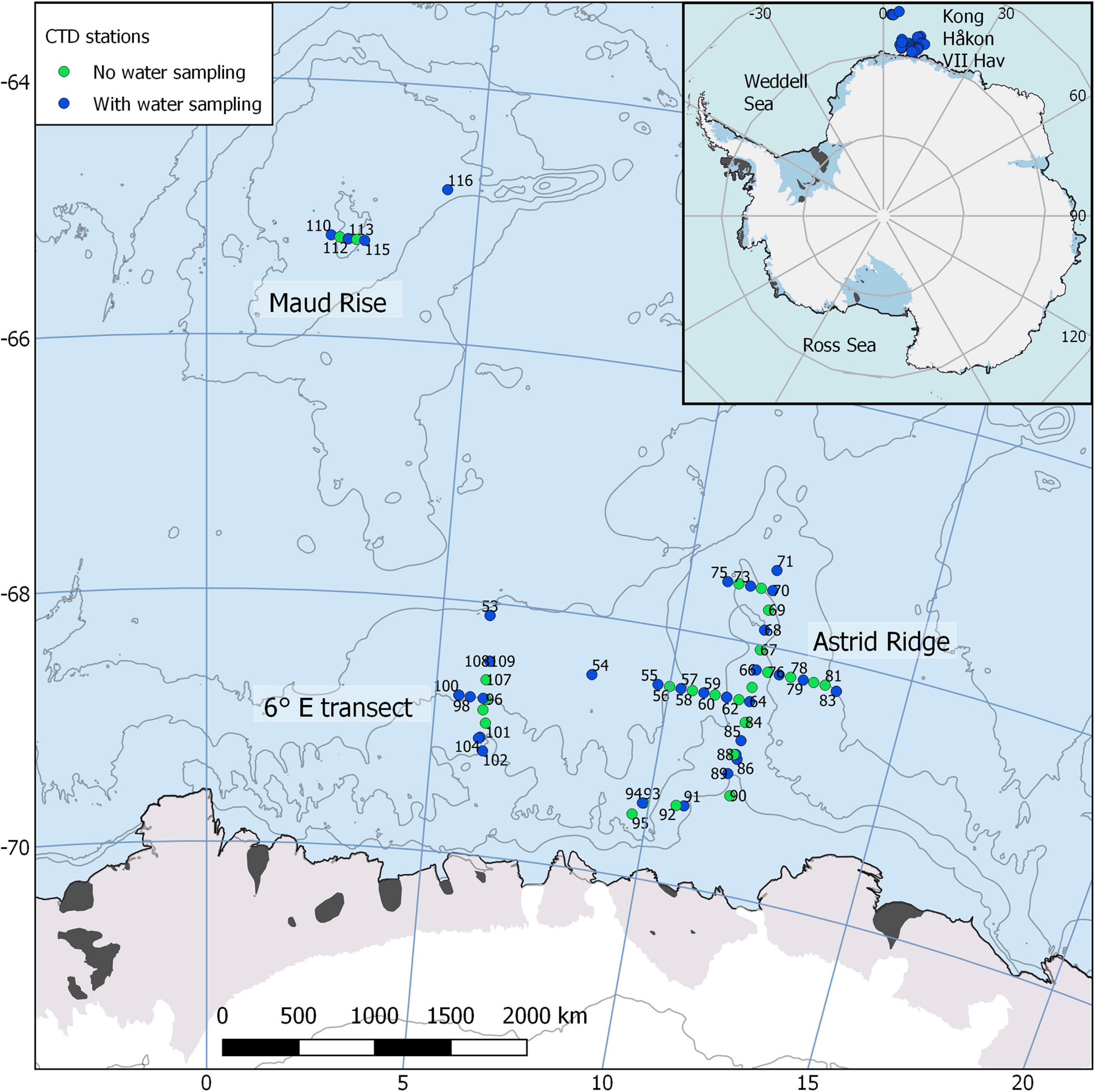
Figure 1. Map of the cruise area, located east of prime meridian in the Kong Håkon VII Hav, showing the sampling stations. Water sampling was conducted at approximately every second station and was focused on the Astrid Ridge, a transect at 6° E and Maud Rise. Map created with the help of Quantarctica (Norwegian Polar Institute, 2018).

To characterize the phytoplankton blooms, water sampling was conducted between 12 and 31 March at 37 stations with station numbers counting upward from 53 (due to continuation of the numbering after a previous cruise). The stations were located between 64.8–69.5° S and 2.3–13.5° E, and the cruise area includes topographic features such as the Maud Rise at circa 3° E and Astrid Ridge at circa 12° E (Figure 1). The main sampling efforts were targeted to Astrid Ridge, a north-south transect at 6° E, and Maud Rise. Water samples were collected with a 24-bottle or 12-bottle SBE 32 carousel water sampler from a multitude of depths.

In addition, during longer transits, water samples were collected every 4 h from the ship’s scientific seawater intake at 4 m depth. Chl a samples were used to calibrate the underway fluorometer (WETStar, Sea-Bird Scientific, with a measurement frequency once per minute) with the equation y = 0.09x + 0.06 (R² = 0.85). Dividing the dataset between day and night time values resulted in very similar equations (y = 0.10x + 0.07 and y = 0.09x + 0.04, respectively).

Chl a samples were filtered (typically 1 L) through 0.7 μm GF/F filters (GE Healthcare, Little Chalfont, United Kingdom) under low vacuum pressure (approximately −30 kPa). Extraction was done with 100% methanol at 5°C in the dark for 24 h (Holm-Hansen and Riemann, 1978). The pigment concentration, including phaeopigments, was measured with a Turner 10-AU Fluorometer (Turner Designs, San Jose, CA, United States) that had been calibrated prior to the cruise.

The abundance of bacteria was determined using an Attune^TM NxT Acoustic Focusing Cytometer (Invitrogen^TM, Thermo Fisher Scientific Inc., United States) equipped with a 50 mW 488 nm (blue) laser. Samples (4.5 mL) were fixed with glutaraldehyde (0.5% final concentration) and stored frozen at −80°C until analysis within 6 months. The samples were thawed and diluted x10 with 0.2 μm filtered TE buffer (Tris 10 mM, EDTA 1 mM, pH 8), stained with SYBR Green I (Molecular Probes, Eugene, OR, United States) at a final concentration of 1:10,000 of the commercial stock solution and then incubated for 10 min in darkness at room temperature (protocol based on Marie et al., 1999). Bacteria were discriminated and counted using biparametric plot based on side scatter and green fluorescence.

Nutrient samples for the analysis of nitrate (NO₃^–), phosphate (PO₄^3–), and silicic acid (Si(OH)₄) were collected into 20 mL vials, fixed with 250 μL of chloroform and stored in fridge until standard analysis at Institute of Marine Research, Bergen, Norway using Autoanalyzer (Skalar) and the spectrophotometric method described in detail in Grasshoff et al. (2009). The detection limits are 0.5 μmol L⁻¹, 0.06 μmol L⁻¹, and 0.7 μmol L⁻¹ for nitrate, phosphate, and silicic acid, respectively.

Chlorophyll a Fluorescence Profiles From CTD Casts

Chl a fluorescence in the water column (in situ) was measured with a WETLabs ECO fluorometer in connection with CTD (conductivity-temperature-depth) casts (SBE911 + system) and water sampling. Data were bin-averaged in 1 m bins. The factory calibration dark count value was corrected to a value chosen by taking the mode of values below 500 m. Sensor sensitivity was adjusted mid-way through the cruise and the data before and after were processed separately. Certain stations (61, 62, and 77 to 86 – corresponding to 12 out of 65 profiles) experienced baseline shifts [the deep value (dark counts) of the fluorescence profiles was lower than in other profiles and compared to the overall mode value]. These were baseline corrected before the calibration and any further analysis by adding the difference between the mode value of the profile in question and the overall mode value. The shift in baseline was, however, minimal and corresponded to 0.03 mg Chl a m^–3.

The baseline-corrected fluorescence profiles were calibrated with the concurrent Chl a water samples. A linear fit was calculated with the help of the dark value defined above and the median of upcast values in a 2 m window around the water sample depth (water samples were taken during the upcast) to obtain a calibration equation (y = 3.05x – 0.05 and y = 0.44x – 0.03 for before and after the sensitivity setting change, respectively). R² was 0.74 and 0.67, respectively. The equation was used to calibrate the downcast values, which are assumed to be most representative of the undisturbed water column and are being used for further analysis. However, the upper 15 m of the water column was thereafter discarded in the analysis of vertical structures due to possible disturbances from the ship.

In high light intensities, the fluorescence signal is affected by algal non-photochemical quenching (cellular processes such as pigment alterations) lowering the proportion of absorbed light that is emitted as fluorescence (Brunet et al., 2011). In the absence of coinciding light backscattering profiles we have corrected for non-photochemical quenching in daytime profiles (based on local sunrise and sunset) by extrapolating the maximum fluorescence value within the MLD to the surface, a method used previously in the Southern Ocean (Xing et al., 2012).

Mixed Layer Depth

Mixed layer depth was defined as the extent of the currently active surface mixed layer, taken as the depth where the salinity (which is determining for density in our environment) increases by 0.01 between two pressure binned values (1 m bin size) after filtering the profile with a 7 pt running median filter to remove spikes. The upper 15 m of the profiles have been disregarded because of spikes in the data and possible disturbances by the ship on the vertical structure of that part of the water column. This criterion essentially uses a density gradient threshold (Holte and Talley, 2009) to identify the surface ocean slab where physical properties such as density, salinity, or temperature are well mixed, i.e., nearly homogeneous with depth (Pellichero et al., 2017).

Zooplankton Sampling and Acoustics

Mesozooplankton was sampled by vertical hauls from 200 m to the surface using a double WP2 (bongo) plankton net (0.25 m², 180 μm mesh size, hauling speed 0.5 m sec^–1). Each sample was split in two halves with a Motoda splitter device. One half of the sample was preserved in 4% borax-buffered formaldehyde-seawater solution, and the other half in 97% ethanol. The abundance and taxonomic composition of zooplankton in the formalin fixed samples were determined using FlowCam (Yokogawa Fluid Imaging Technologies, Inc., Japan) (Sieracki et al., 1998). The samples were washed and diluted with 2750 ml of fresh-water, kept suspended using an overhead stirrer and imaged using a FlowCam macro (0.5 × objective, 10 mm × 5 mm flow-cell, and a flow rate of 375 ml min^–1). We applied the automatic image segregation and feature extraction procedure described by Álvarez et al. (2012) and created our training set and classifier using the r-package Zooimage (Grosjean and Denis, 2014; Vu et al., 2014). The classifier was based on a random forest machine learning algorithm and had an error rate of 12% determined by 10-fold cross validation.

Krill was studied with the help of echosounding. The acoustic equipment in use was Simrad EK80 research echosounder with six frequencies. The 38 kHz was scrutinized for this study. Scrutinization was done in LSSS (Korneliussen et al., 2016) version 2.5.0. There were two transducers on the research vessel, one on the drop-keel (3 m from hull when down) and one hull-mounted. In ice-covered areas it was not possible to have the drop-keel lowered, and the hull-mounted transducer was in use in these areas. Sea ice and the use of the hull-mounted transducer may have considerably affected registrations in depth but can be assumed to have minor effect on registrations of krill swarms, as they occur in relatively shallow waters. Krill density is given as nautical area scattering coefficient (NASC), which expresses integrated amounts of the acoustic echo that is assigned to krill and can be viewed as proportional to abundance (Maclennan et al., 2002).

Phenology Indices

Bloom Phenology

To include adjacent areas in all directions for context of the cruise area (Figure 1), remote sensing products are presented between 10° W and 50° E and 60° and 71° S, which also includes the Gunnerus Ridge at ca. 35° E, hereafter referred to as the study area.

Level 3 Chl a satellite remote sensing data from Ocean Colour Climate Change Initiative dataset (OC-CCI), version 4.2 (European Space Agency, available online at http://www.esa-oceancolour-cci.org; Sathyendranath et al., 2019, 2020) in 8-day and 4 km resolution were used for bloom phenology studies. The data span from September 1997 to March 2020 and are merged from several sensors including SeaWIFS, MODIS, MERIS, and VIIRS. To test the reliability of the OC-CCI product in such high latitude environment, we ran a similar analysis with the unmerged products from SeaWIFS and MODIS (results not shown). This yielded similar results for bloom timing indices than with the OC-CCI (the bloom amplitude was somewhat higher but in the same range). The OC-CCI product was, therefore, chosen as the main data product due to its continuity in time, higher spatial and temporal coverage, and the uncertainty estimates provided with the data.

The performance tests for OC-CCI (Sathyendranath et al., 2019) indicated that sea ice is masked effectively (99.9% of sea ice/snow pixels classified as sea ice/snow or clouds; their Table 3). However, sea ice can also affect values in nearby pixels due to the adjacency effect (reflectance from the nearby pixels containing sea ice affects the remote sensing reflectance retrieval for the pixel in question through atmospheric scattering) for up to 20 km distance (Bélanger et al., 2007). To account for this, we masked out the adjacent pixels to sea ice. Sea ice concentration (see section “Sea Ice Phenology” for details) from the beginning of each satellite week was interpolated to match the Chl a data coordinates and concentrations above 15% were classified as ice-containing pixels. Thereafter, five pixels (corresponding to ∼20 km) in each direction from the ice-containing pixels were excluded from the Chl a dataset before further analysis.

The uncertainty estimates for the OC-CCI product indicated higher uncertainty in the data along the coast (Supplementary Figures 1A,B). The root mean square deviation (RMSD) values are here constantly elevated and higher than the range for the different optical water classes presented in the Figure 4 of Sathyendranath et al. (2019). In addition, an early analysis showed anomalous phenology index values in these areas (not shown). Therefore these areas were permanently excluded from the analysis (Supplementary Figure 1C). To do so, the long-term means of RMSD were first calculated for each satellite week. The maximum geographical appearance of out-of-range values (compared to the Figure 4 of Sathyendranath et al., 2019) in areas close to the coast (areas with less than 3000 m bottom depth south of 66°S) was masked before further analysis (that is, the maximum of the weekly means for each pixel was considered for the comparison with the Figure 4 values). For large parts of the year, these areas are already masked because of sea ice.

FIGURE 2

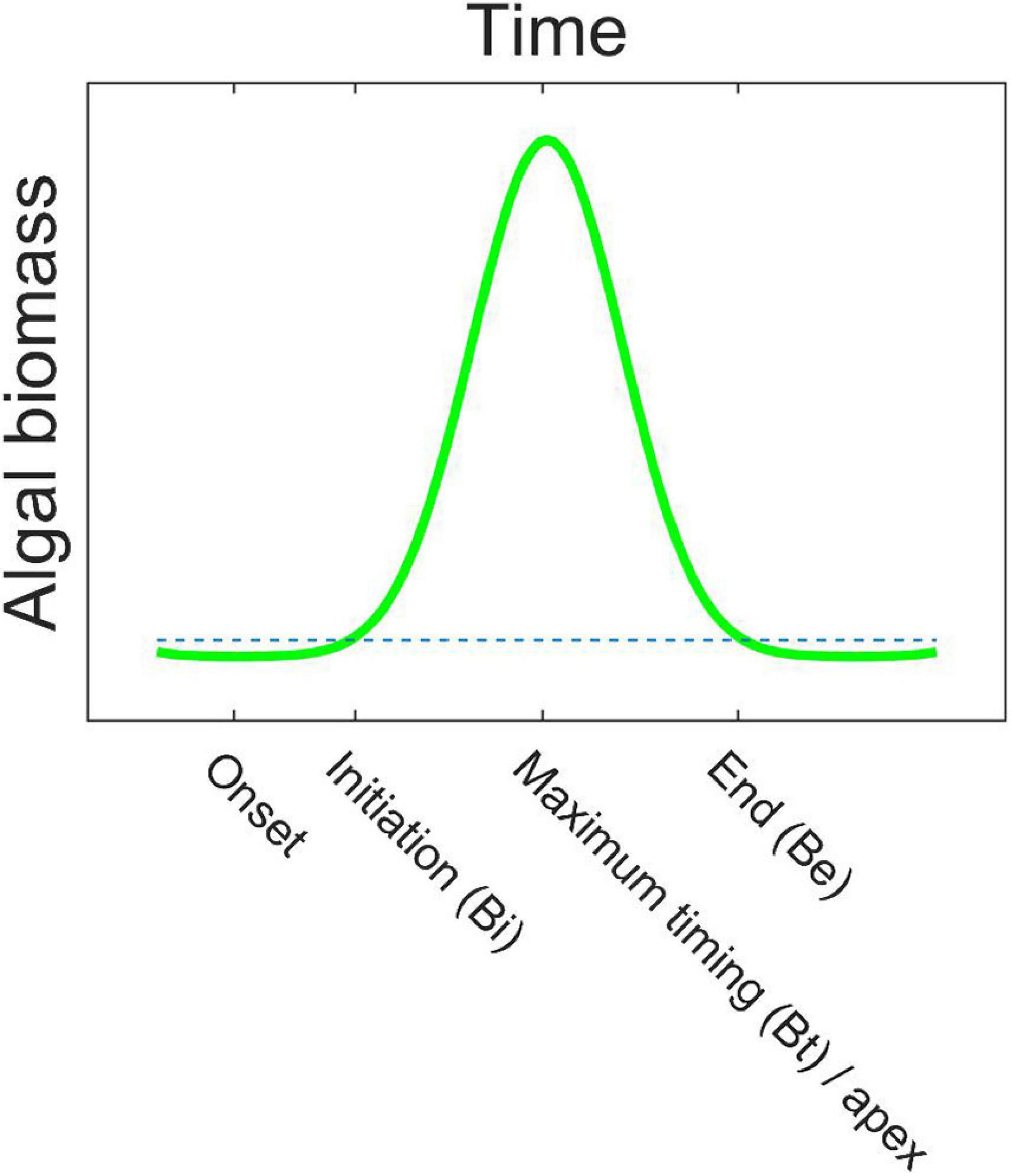
Figure 2. An idealized bloom with the bloom phenology indices bloom onset, initiation (Bi), timing of maximum concentration (Bt)/apex, and end (Be) indicated. The stippled line is the 1.05 times median threshold. See Table 1 for further index explanations.

FIGURE 3

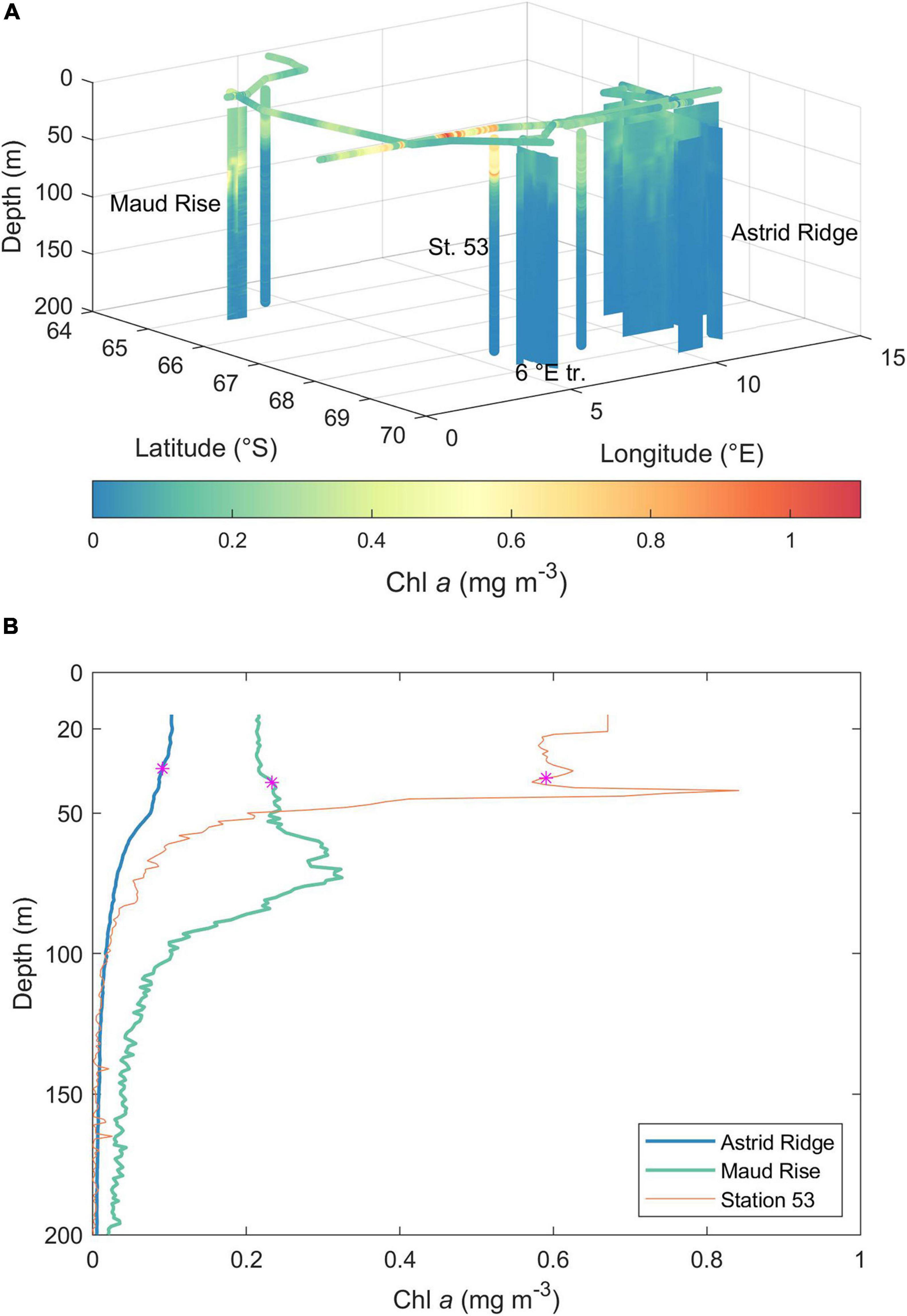
Figure 3. (A) Chl a concentration during the cruise, as obtained from calibrated in situ fluorescence profiles and underway fluorescence measurements. See map (Figure 1) for 2D orientation of the sampling locations. St. 53, station 53; 6°E tr., 6°E transect. (B) Mean Chl a profiles of Astrid Ridge and Maud Rise stations and the profile from station 53. The magenta star shows the MLD (mean for Astrid Ridge and Maud Rise).

FIGURE 4

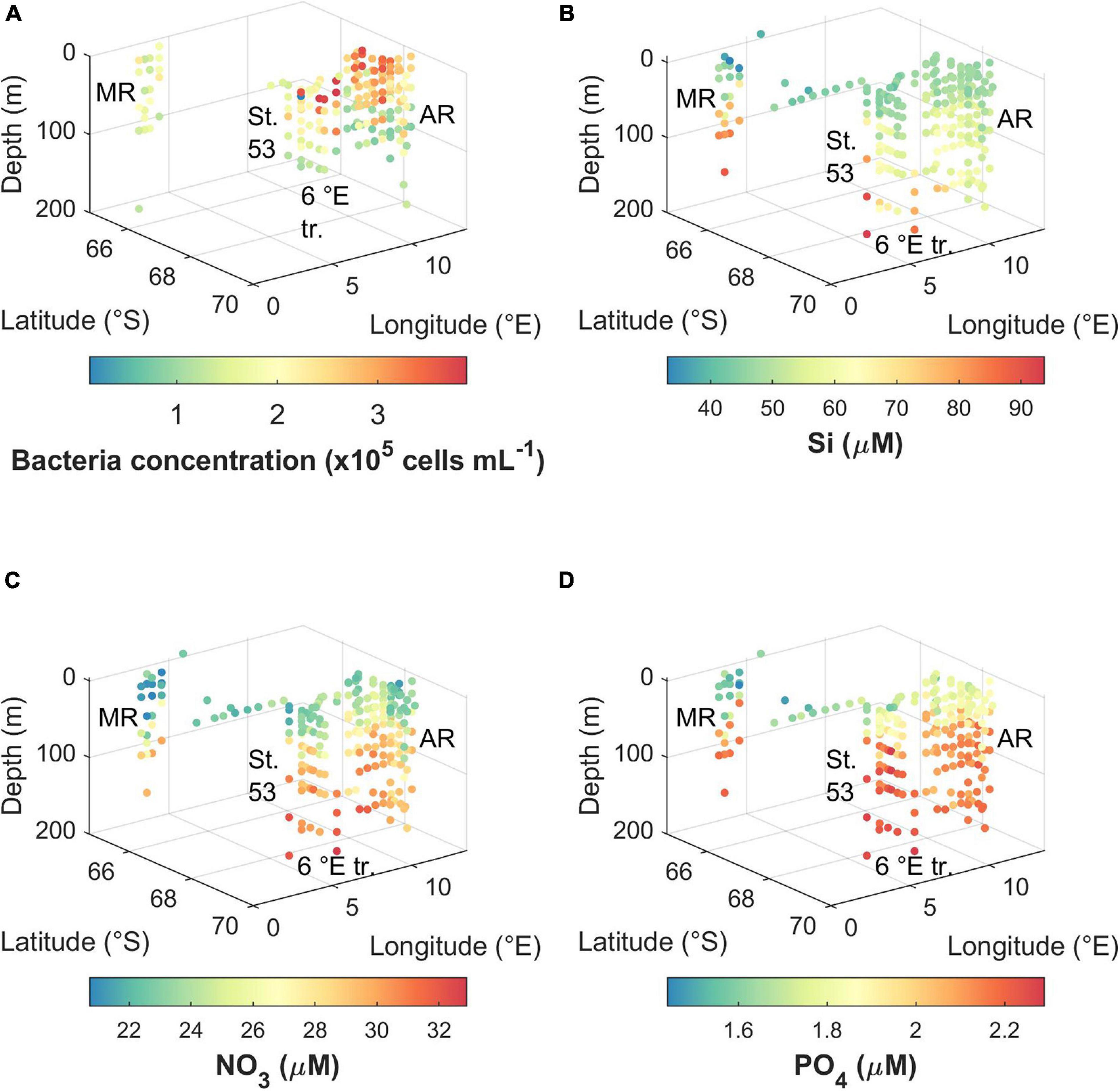
Figure 4. Concentration of (A) bacteria, (B) silicic acid, (C) nitrate, and (D) phosphate during the cruise. MR, Maud Rise; St. 53, station 53; 6°E tr., 6°E transect; AR, Astrid Ridge.

A year in this context is from July to June to include the Southern hemisphere productive season (i.e., Austral summer) within 1 year. As the Austral winter months lack data for a long period, the exact choice of start date for the year is not relevant. However, phenology results are reported with satellite week numbers corresponding to the beginning of a calendar year for easier interpretation (e.g., satellite week 1 starts January 1st). We have followed the methodology of the global bloom phenology study by Racault et al. (2012). To reduce gaps in the data, a spatial median filter (3 by 3 pixels) was applied to missing pixels. Thereafter, if a pixel was still empty, an average of the week before and after (if both contained data in the original, non-interpolated matrix) was taken. To smooth spikes in the data a 3-week moving median filter was applied to the pixels that contained data (that is, empty pixels were maintained in this step and no interpolation was done). Thus, the interpolation filled gaps of maximum 1 week. The effect of the interpolation methods on the phenology results is shown in Supplementary Figure 2 and discussed in section “Methodological Challenges.”

We used a relative threshold -based approach as the bloom detection method, where the threshold was set to 1.05 times the annual median, which is a commonly used method (e.g., Racault et al., 2012; and for the Southern Ocean see Thomalla et al., 2011; Soppa et al., 2016). The used bloom phenology indices are defined in the following text, summarized in Table 1, and a selection is shown on a bloom schematics in Figure 2. To determine bloom initiation (Bi), the Chl a concentration had to exceed the threshold for at least 2 consecutive weeks. Bloom end (Be) was determined when the concentration for the last time exceeded the threshold on at least 2 consecutive weeks. The “first” bloom initiation and the “last” bloom end were recorded – i.e., if the concentration would fall below the threshold in between, this was not considered (a single bloom is characteristic for the Southern Ocean annual phytoplankton cycle; Arrigo et al., 2008; Ardyna et al., 2017). The bloom duration (Bd) is the time between bloom initiation and bloom end. In addition, maximum concentration (bloom amplitude, Ba), its timing (Bt), and the average concentration during the bloom (Bm) were calculated. For all the indices, a mean over all the years (23) is presented, called the long-term mean hereafter. To test the sensitivity of the bloom initiation results to the choice of detection method, we further tested a method based on the rate of change in the Chl a concentration (bloom initiation Bi_r), as outlined in the Supplementary Material section 2.

TABLE 1

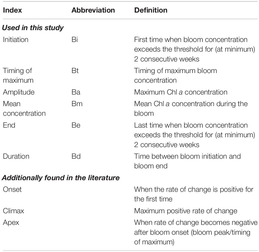
Table 1. Bloom phenology indices calculated for a given Austral year (i.e., July to June).

Cole et al. (2012) highlighted problems in the phenology studies arising from gaps in the data. This is especially true in the Southern Ocean where the calculated bloom initiation is likely to be found later than the true bloom initiation because the absence of winter data increases artificially the annual median and, thus, the threshold (Cole et al., 2012). For our results, where the exact date is of importance (in comparison with sea ice phenology), the consequences of biases are discussed (see also section “Methodological Challenges”). Even though we have interpolated the data to reduce the gaps (see above), austral summer data still has gaps with about 42–62% of pixels missing for a given week in January–February (average over all the years; including the permanently masked areas; Supplementary Figure 3). However, for the long-term means of the bloom phenology indices, the geographical pattern is not altered as we apply a rule that half of the years must contain index data for the mean to be calculated for a given pixel. In this case, the phenology indices were calculated for the vast majority of pixels (73%, where the 27% contain the permanently masked coastal areas).

The phenology index maps were drawn with the Matlab package M_Map (Pawlowicz, 2020) with colormaps from Thyng et al. (2016). For the “Discussion” section, a schematics figure was created to make regions with differing phenology index characteristics visible and to function as a schematics of the regional bloom regimes. Bloom mean concentration and bloom end maps were created with a blue-red diverging color map and a composite image of the two images was thereafter created with the Matlab Image Processing Toolbox (imfuse). The color gradient thus does not have a quantitative meaning.

Sea Ice Phenology

Daily sea ice concentration data in 25 km resolution from the National Snow and Ice Data Center (Cavalieri et al., 1996; updated yearly) from the years 1997 to 2019 were used to calculate the sea ice phenology. A year in this context was defined from 1st of February to the following 31st of January because the Austral summer sea ice extent minimum occurs in February. For sea ice phenology indices we followed the methodology used in Stammerjohn et al. (2008) for the waters west of the Antarctic Peninsula. Each year, sea-ice advance was defined for each pixel as the time when sea-ice concentration exceeded 15% for 5 consecutive days. Similarly, the sea-ice retreat was defined when sea-ice concentration was for the last time in a given year above 15% for 5 consecutive days. If the sea-ice concentration was never below 15% for a given pixel, the day of advance was set as the first day of a year, and the day of retreat as the last day of a year. The sea-ice period is the time between advance and retreat, and the sea-ice persistence is the percentage of time (days) when the sea-ice concentration is above the threshold within the sea-ice period. If the concentration was never above the threshold for 5 consecutive days, these indices (sea-ice period and sea-ice persistence) were set to 0.

To compare the timing of sea ice retreat and advance with the phytoplankton blooms, the sea-ice phenology indices were re-gridded (via interpolation) to the coordinates of the bloom phenology indices, and the temporal resolution was reduced to 8-day “weeks” (all days belonging to a given satellite week were given that week number). Difference between the sea-ice and bloom timings indicated by the long-term means is presented here. For sea ice retreat and bloom initiation, 3 satellite weeks was chosen in the figures as the cut-off value for the timing difference to indicate dependence (cf. Perrette et al., 2011). Altering the sea-ice concentration threshold between 5 and 30% did not change the overall geographical pattern in the time difference between sea ice retreat and bloom initiation (not shown) so it is a robust method.

Data Products: Euphotic Depth, Photosynthetically Available Radiation, Mixed Layer Depth, Tides and Currents

Euphotic depth (ZEu, m) and daily incident irradiance in the photosynthetically available radiation range (PAR, 400–700 nm; mol m^–2 day^–1; Frouin et al., 2003) satellite remote sensing data products were obtained from merged products by GlobColour¹ in 8-day resolution in the time frame 1997–2020. ZEu is based on satellite-derived Chl a concentration and the 1% PAR threshold (Morel et al., 2007). Weekly means (for 8-day satellite weeks) were calculated over the time series to obtain the seasonality.

MLD for Southern Ocean were obtained from Pellichero et al. (2017). The MLD climatology is estimated with monthly and half a degree resolution based on elephant seal-derived, ship-based, and Argo float observations. The amount of data from the different data sources and for the different areas is shown in their Figure 1, with areas around the prime meridian and Gunnerus Ridge having the best coverage in the study area. To study the light conditions for phytoplankton and compare ZEu with the MLDs, monthly means were calculated for ZEu, and MLD was interpolated to fit the coordinates of ZEu.

To assess the role of tidally induced mixing for bloom magnitude, maps of tidal kinetic energy were derived from a regional configuration of the ice shelf-augmented version of the Finite Volume Community Ocean Model (FVCOM; Zhou and Hattermann, 2020), which covers a zonal and meridional extent of about 4000 km × 4000 km of the wider Weddell Gyre circulation in the Atlantic sector of the Southern Ocean, while at the same time resolving the Kong Håkon VII Hav and Dronning Maud Land continental shelf break regions at mesh resolution of down to 1.5 km. The model is initialized and forced along the open boundary with results from the circumpolar metROMS solution of Naughten et al. (2018) and time series of tidal elevation from the TPXO global inverse barotropic tidal solution (Egbert and Erofeeva, 2002). Patterns of tidal elevation and current amplitudes from this model resemble the results from the Antarctic inverse barotropic tidal CATS2008b, an update to the model described by Padman et al. (2002, 2008), albeit showing a more detailed spatial structure in our study region and explicitly resolving the interaction of the tides with the background stratification that has been highlighted to be important along the Antarctic continental shelf break (Flexas et al., 2015; Stewart et al., 2019).

To assess the general ocean current patterns in the area, maps of L4 monthly means of mean kinetic energy (MKE) and surface current velocities were retrieved from Copernicus Marine Services (global ocean reanalysis product available at https://resources.marine.copernicus.eu/?option=com_csw&view=details&product_id=GLOBAL_ANALYSIS_FORECAST_PHY_001_024). Data were available from January 2016 to December 2019 in 1/12° resolution.

Results

Cruise Observations

The highest Chl a concentrations in the vertical in situ fluorescence profiles were observed at the open-ocean CTD station 53 at 68.1° S and 6.0° E and at Maud Rise (Figure 3). In the former, Chl a was concentrated in the upper 50 m with a deep maximum of 0.84 mg Chl a m^–3 (at 42 m), whereas at Maud Rise, the highest Chl a concentrations were found below 50 m, with a maximum of 0.70 mg Chl a m^–3. Astrid Ridge and the 6°E transect CTD stations were characterized by low Chl a concentration, with maxima of 0.25 and 0.16 mg Chl a m^–3, respectively. The underway fluorometer measured somewhat higher values, up to 1.1 mg m^–3, in the area west of the station 53.

Bacterial abundance was highest in the east and south of the cruise area, i.e., at Astrid Ridge and the 6° E transect CTD stations, as well as at a station at 68.5° S and 8.3° E (CTD station 54), with maximum concentration of 3.8 × 10⁵, 3.9 × 10⁵, and 3.9 × 10⁵ cells mL^–1, respectively (Figure 4A). The maximum concentration at Maud Rise and CTD station 53 was 2.3 × 10⁵ and 2.6 × 10⁵ cells mL^–1, respectively. Surface values were typically higher than deeper samples at the east and south stations while the abundance was more uniform at the west and north stations.

Macro-nutrient concentrations are shown for the upper 200 m (Figures 4B–D). The main features are differences between upper water column and deep values, and differences between the areas, especially regarding Maud Rise compared to the other sampling areas. The concentrations were in general lowest near the surface. For the CTD stations (upper 200 m), silicic acid ranged between 43.5 and 93.8 μM, nitrate ranged between 20.7 and 32.9 μM, and phosphate ranged between 1.5 and 2.3 μM. When including the underway samples, the lowest concentration for silicic acid was 33.0 μM and for phosphate 1.4 μM. The lowest values were observed at Maud rise except for the CTD station-based silicic acid minimum, which was at the 6° E transect. However, in general Maud Rise appears to have the smallest surface reservoirs, followed by the station 53. Regarding nitrate values at Astrid Ridge, the south-east had the lowest values.

Acoustic observations of euphausiids showed highly heterogeneous distributions across the study area (Figure 5A). The largest patches of krill swarms (Euphausia superba) occurred in the northernmost part of the 6° E transect (yellow – red colors in the figure). Patches of euphausiids were also found at Astrid Ridge (green colors), but hardly at Maud Rise. Euphausiid larvae were also observed in net tows mainly outside of Maud Rise. Mesozooplankton abundances in upper 200 m were, on contrary, highest at Maud Rise, both in terms of numbers (960–2300 N m^–3; Figure 5B) and biomass (0.06–0.14 g m^–3). Abundances at Astrid Ridge and 6° E transect stations were generally lower, ranging from 330 to 1100 N m^–3 (0.08–0.02 g m^–3). The zooplankton community was characterized by a large proportion of small sized copepods (180–1000 μm), nauplii and protists.

FIGURE 5

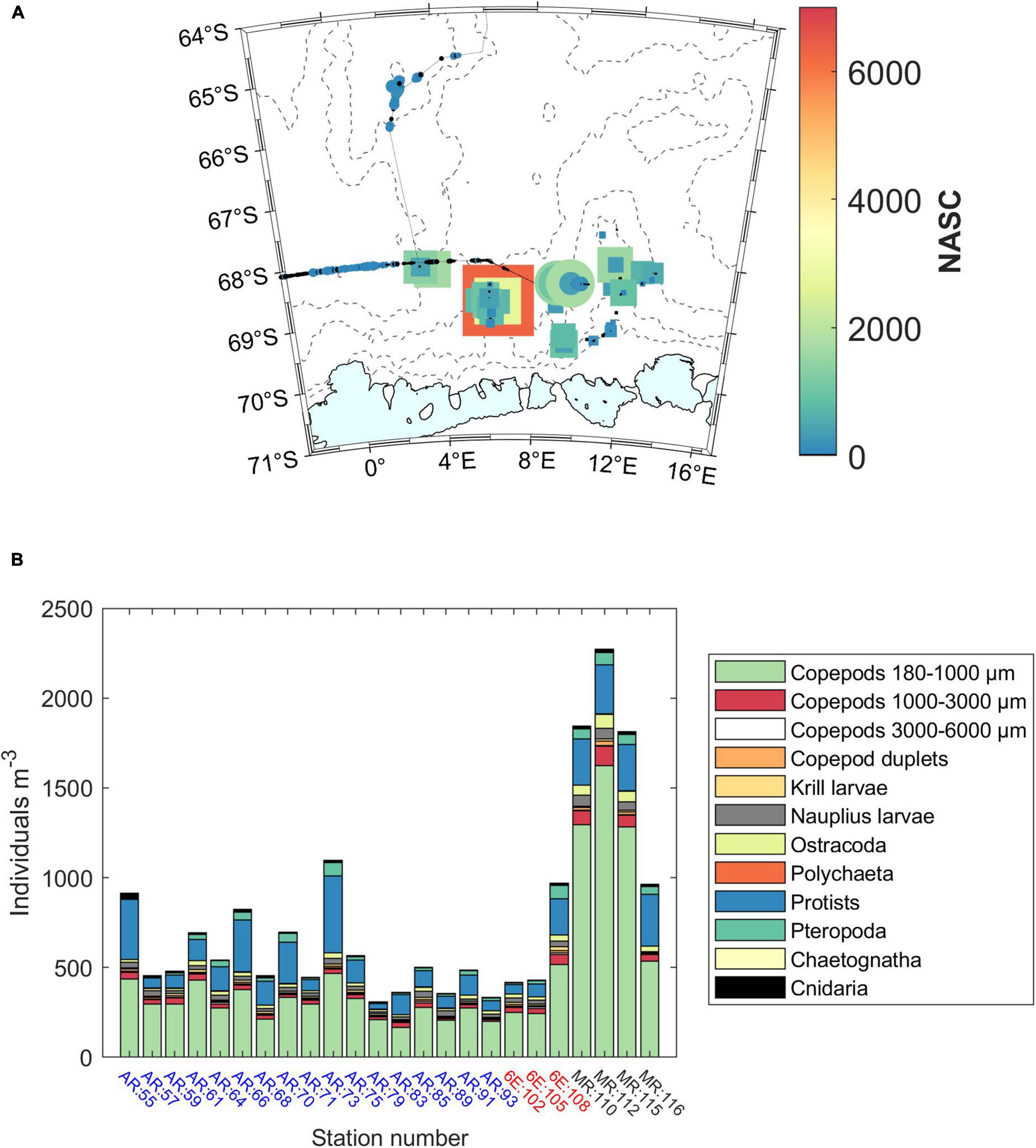
Figure 5. (A) Acoustic observations of krill. Each marker represents the nautical area scattering coefficient (NASC) values integrated over 500 m distance, with size proportional to the value and color expressing the exact values (see color scale bar for values). Round symbols are used when data were retrieved with the drop-keel transducer, while square symbols are used when data were retrieved with the hull-mounted transducer. The hull-mounted transducer was used in ice-covered/ice-edge areas. (B) Abundances of different mesozooplankton groups obtained with the FlowCam. Astrid Ridge (AR) stations are numbers 55 to 93 and marked with blue; 6°E transect (6E) stations are numbers 102 to 108 marked with red, and Maud Rise (MR) stations are numbers 110 to 116 marked with black. Copepod duplets are images where two copepods are overlapping and can thus not be taxonomically classified.

MLDs in the different sampling areas were on average (±standard deviation) 38, 34 (±14), 33 (±8), and 39 (±13) m for station 53, Astrid Ridge, 6° E transect and Maud Rise, respectively (Figure 3B). Average MLD of all stations was 36 (±13) m.

Bloom Phenology

In this section, results based on the long-term means of the phenology indices are presented. Blooms initiate during January in the majority of the study area (satellite weeks 1–4, January 1st to February 1st; Figure 6A). A band around Astrid Ridge initiates in late January – early February. Bloom initiation is in general earlier in the north than in the south, with especially the western area showing a distinction between near-slope and off-slope, open-ocean areas. The bloom initiation results based on the rate of change method are outlined in Supplementary Material section 2 and are largely similar in that blooms initiate mainly in January, but with a somewhat different geographical pattern.

FIGURE 6

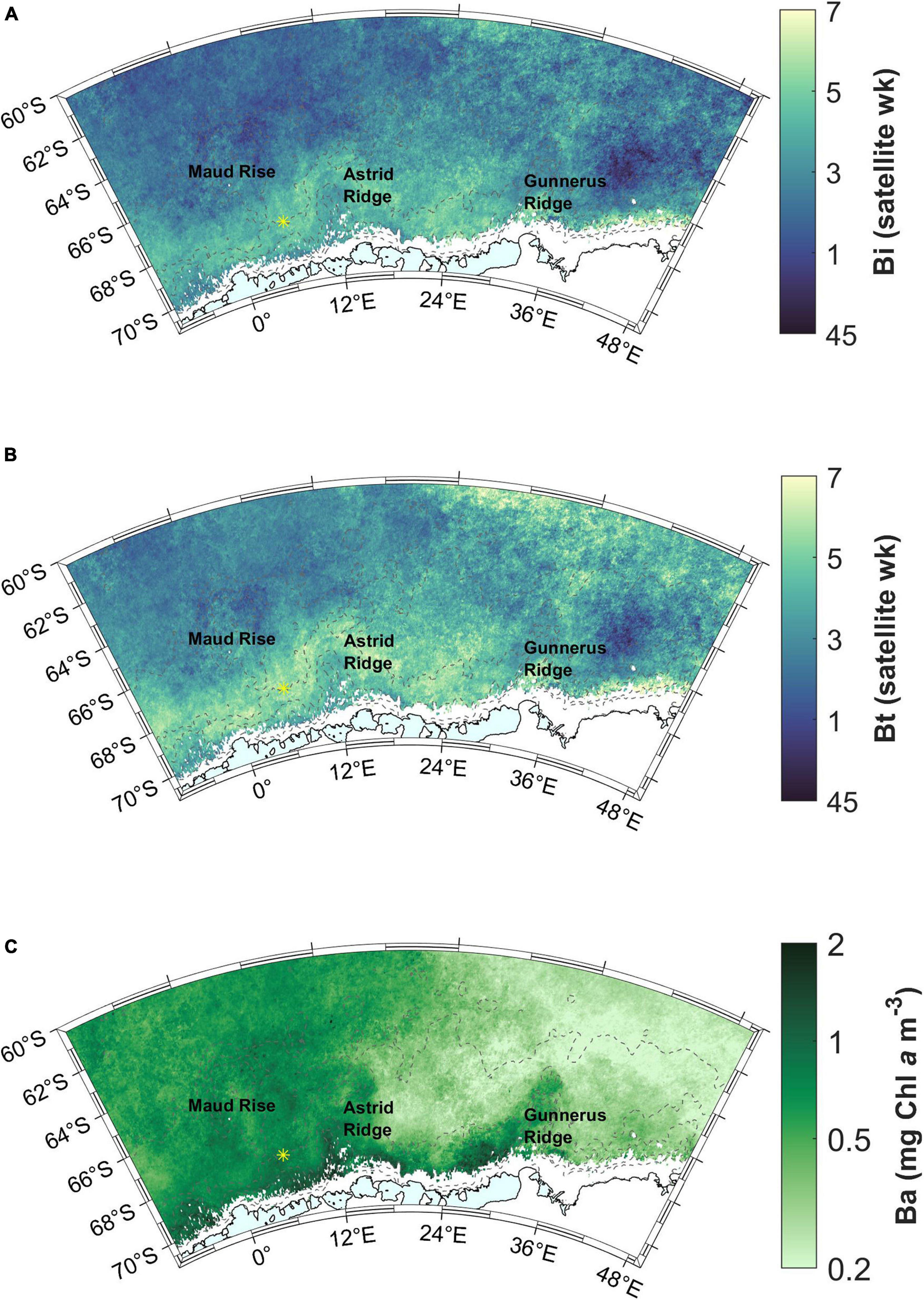
Figure 6. (A) Bloom initiation (Bi) across the study area. (B) Timing of the bloom maximum concentration (Bt). Satellite week 1 starts on January 1st (there are 46 8-day “satellite weeks” in a year). Satellite week 5 starts on February 2nd. (C) Bloom amplitude (Ba). Station 53 is shown with a yellow asterisk.

The timing of the maximum Chl a concentration during the bloom follows a similar geographical pattern to that of the bloom initiation, with the latest occurrences on and around Astrid Ridge and in the north-east corner of the study area (Figure 6B). The latter corresponds to the areas indicated as the southern boundary of the ACC and the southern ACC Front (Orsi et al., 1995), hereafter referred to as southern ACC.

The maximum Chl a concentration, i.e., bloom amplitude, is highest on a band starting west of Gunnerus Ridge and extending west past Astrid Ridge, and in general on the western side of the study area, with values in the order of 0.5–2 mg m^–3, (Figure 6C). The blooms terminate in the end of January or during February (before satellite week 8, starting February 26th; Figure 7A). A band around Astrid Ridge, and the southern ACC have the latest bloom end in February. Bloom duration is thus 2–4 satellite weeks in the majority of the study area (Figure 7B), but longer in southern ACC lasting between 4 and 7 satellite weeks.

FIGURE 7

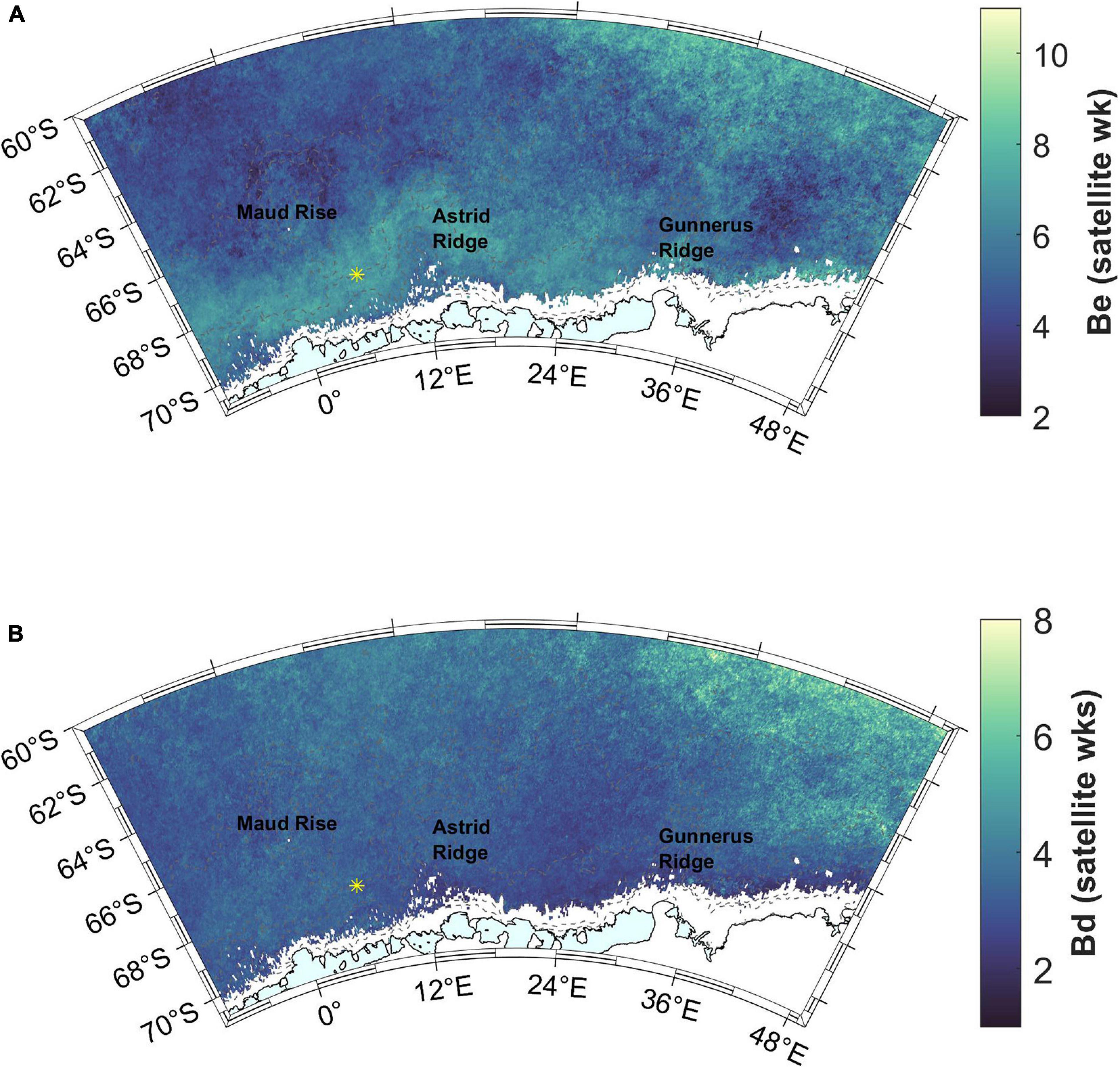
Figure 7. (A) Bloom end (Be). Satellite week 5 starts on February 2nd and satellite week 8 on February 26th. (B) Bloom duration (Bd). Station 53 is shown with a yellow asterisk.

Regarding the variability of the long-term means, standard deviations (Supplementary Figure 4) are below 4 satellite weeks for the timing indices (bloom initiation, end and maximum timing) in the majority of the study area, with southern ACC having the highest variability, whereas they are lower for the bloom duration (predominantly below 2 satellite weeks, except for the southern ACC). As such, although blooms may thus occur at somewhat different times in different years, they will have a similar bloom duration. Regarding bloom magnitude, standard deviations are highest (slightly above 1 mg Chl a mg^–3) in the areas where the highest Chl a concentrations are found, which indicates that the productive areas may have weak blooms in some years.

Sea Ice Phenology and Relation to Bloom Phenology

The whole study area is seasonally ice-covered with high (>90%) sea ice persistence (Figure 8A). Sea ice retreat is in December (between days 335 and 365) in large parts of the study area, with an earlier retreat at the southern ACC and a later retreat along the coast (Figure 8B). Maud Rise shows an earlier sea ice retreat than the surrounding areas. Sea ice advance is before March (before day 60) very close to the coast, and is gradually later further north (Figure 8C). The areas around and between Astrid and Gunnerus Ridges and the majority of Maud Rise have sea ice advance before June (before day 150), whereas the northern parts have even later sea ice advance. Standard deviations of the long-term means are shown in Supplementary Figure 5 and are fairly low and uniform across the study area except for sea ice advance that has higher variability along the coast (standard deviation more than 30 days).

FIGURE 8

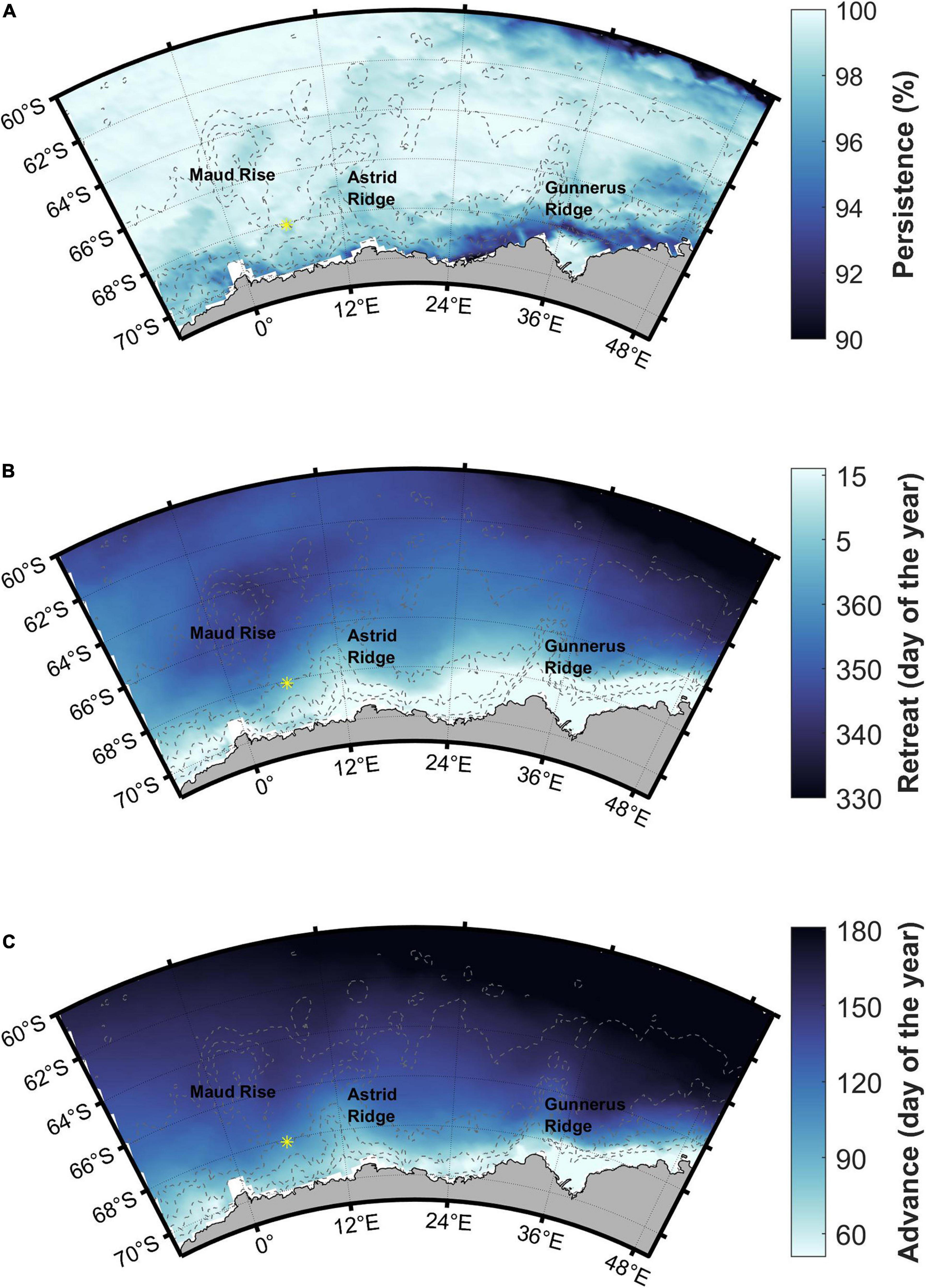
Figure 8. Sea ice (A) persistence, (B) retreat, and (C) advance. Station 53 is shown with a yellow asterisk.

The blooms follow the sea ice retreat by less than 3 satellite weeks (24 days) in areas close to the coast (red areas in Figure 9A). Some other, smaller areas, especially west of Maud Rise, also fall within this time limit, whereas in large parts of the study area a longer time period elapses between sea ice retreat and bloom initiation. Especially the southern ACC shows a long time gap between sea ice retreat and bloom initiation, 6–8 satellite weeks, i.e., about 2 months. According to the rate of change method, a larger area in the west of the study area (around Maud Rise) falls within the time limit of 3 satellite weeks (Supplementary Material section 2).

FIGURE 9

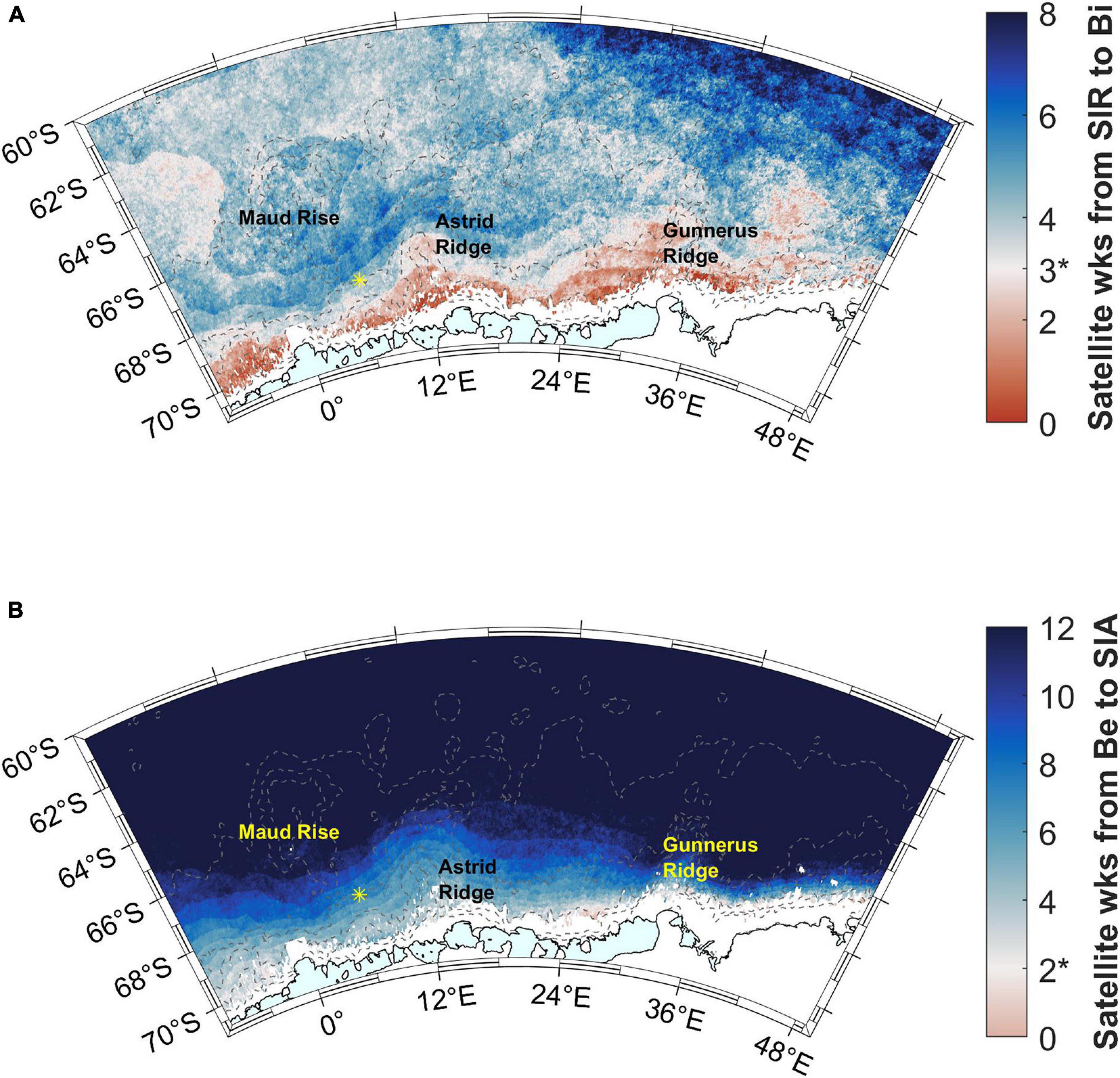
Figure 9. (A) Time (in 8-day satellite weeks) from sea ice retreat (SIR) to bloom initiation. Time difference of 3 satellite weeks is highlighted with a color change and asterisk in the color scale legend (see the text for choice of the time period). (B) Time (in 8-day satellite weeks) from bloom end to sea ice advance (SIA). Time difference of 2 satellite weeks is highlighted with a color change and asterisk in the color scale legend. Station 53 is shown with a yellow asterisk.

Blooms end well before sea ice advance (more than 2 satellite weeks, i.e., 16 days) almost everywhere in the study area (blue areas in Figure 9B). For areas outside of the coastal ridges, this time gap is more than 10 weeks.

Light and Mixed Layer Depth

The annual maximum ZEu (study area average 138 m) and PAR (study area average 41 mol m^–2 day^–1) mainly occur before January, i.e., before the blooms; whereas ZEu is shallowest (study area average 60 m) mainly after that, i.e., during the blooms (not shown). For comparison with the MLD data, monthly means of ZEu were calculated. ZEu averaged for the entire study area for November, December, January, February, and March is 108 (±19), 78 (±13), 68 (±12), 72 (±10), and 80 (±8) m, respectively. The day length at the end of February in the study area is above 14 h (as calculated from the NOAA Solar Calculator)².

Mixed layer depth is shallowest in December fairly uniformly across the area (Figure 10A) and ranges between 15 and 75 m (Pellichero et al., 2017). The MLD averaged for the entire study area for November, December, January, February, and March is 56 (±21), 25 (±6), 27 (±5), 37 (±6), and 49 (±9) m, respectively. When comparing March values from this product to the estimated MLDs from the cruise (coordinates of the latter ones rounded to the nearest whole degree), the MLD product values are on average 10 (±13) m deeper than the cruise values (range from 33 m deeper to 28 m shallower). This may suggest that the comparison to ZEu is a conservative estimate regarding light availability. Especially the Maud Rise stations during the cruise had deeper MLDs than the MLD product, whereas the opposite was true for Astrid Ridge and 6°E transect, which may in part reflect the sampling time: Maud Rise was sampled at the very end of the month, and the MLD product has a monthly resolution.

FIGURE 10

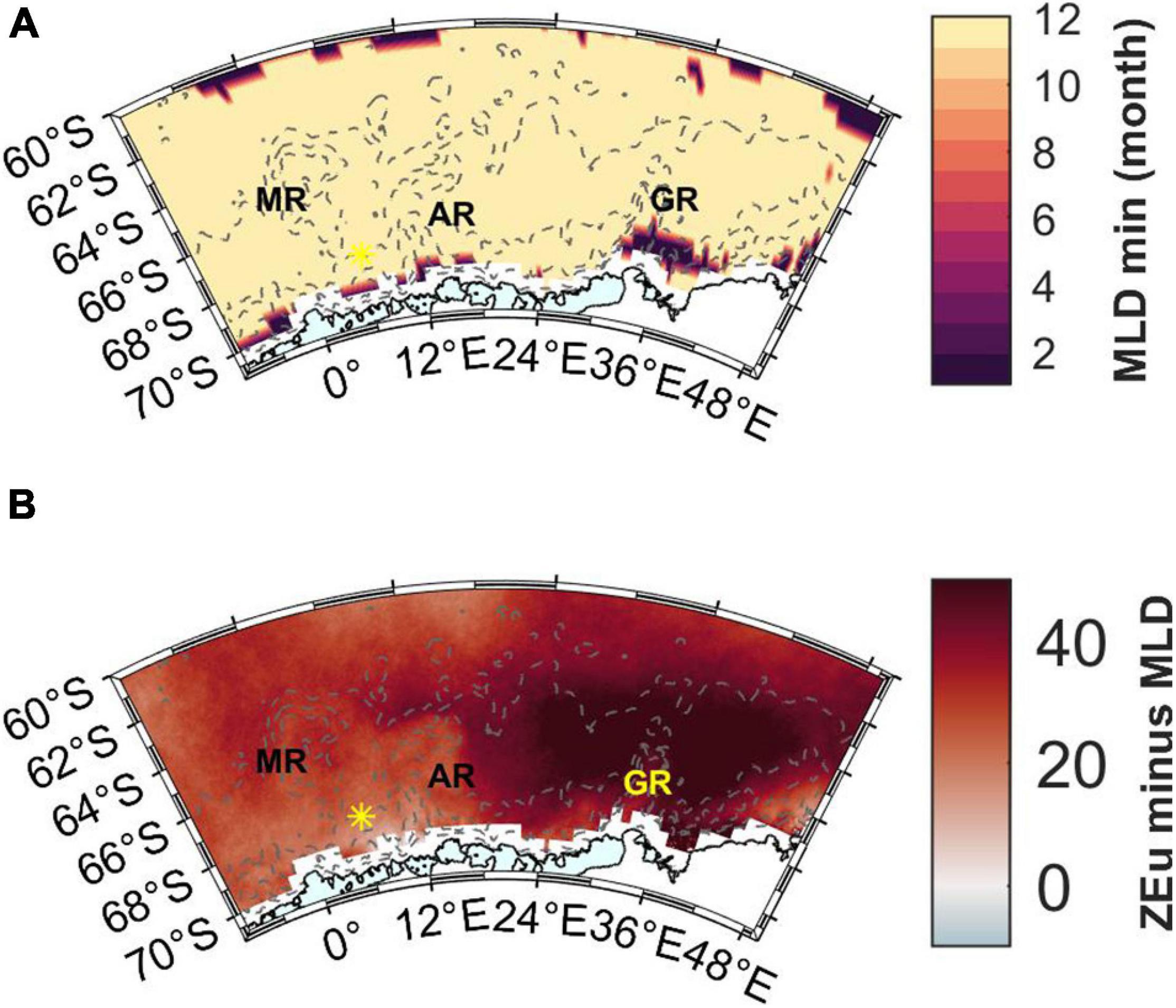
Figure 10. (A) The month in which the annual minimum MLD occurs according to the data product by Pellichero et al. (2017). (B) Light availability expressed as the difference between ZEu and MLD in February. Red color indicates that MLD is shallower than ZEu. MR, Maud Rise; AR, Astrid Ridge; GR, Gunnerus Ridge. Station 53 is shown with a yellow asterisk.

ZEu is deeper than the MLD throughout the productive season and across the study area (only February is shown in Figure 10B) thus indicating sufficient light availability. ZEu is affected by the algal biomass and shows geographical differences with shallowest values in the western part of the study area (resulting in smaller differences between ZEu and MLD), however, ZEu is still deeper than MLD.

Ocean Currents

Tidal currents along the coast are highest at the base of both Astrid and Gunnerus Ridges (Figure 11A). The highest MKE occurs along the coast, indicating the Antarctic Slope Current (Figure 11B). The current direction in the Antarctic Slope Current is from east to west, based on the surface current velocity vectors. Both these patterns coincide with the areas of the highest bloom magnitude (Figures 6C, 11C), where the area east of Gunnerus Ridge has throughout low bloom magnitude and the area east of Astrid Ridge has low bloom magnitude in areas away from the coast. Conditions for high productivity are thus met at the west side of Gunnerus Ridge, then transported by the westward flowing Antarctic Slope Current, and further amplified at Astrid Ridge. Small coastal areas at Gunnerus and Astrid Ridges have the highest bloom mean concentration values (>1 mg Chl a m^–3; Figure 11C). The western part of the study area (north and west of Astrid Ridge), also have a considerable mean concentration during the bloom (>0.5 mg Chl a m^–3), whereas the eastern part of the study area shows low values (<0.5 mg Chl a m^–3). MKE is elevated also in the north-eastern corner of the study area, indicating the southern ACC. Somewhat higher values can also be seen around Maud Rise, corresponding to the area with medium bloom magnitude.

FIGURE 11

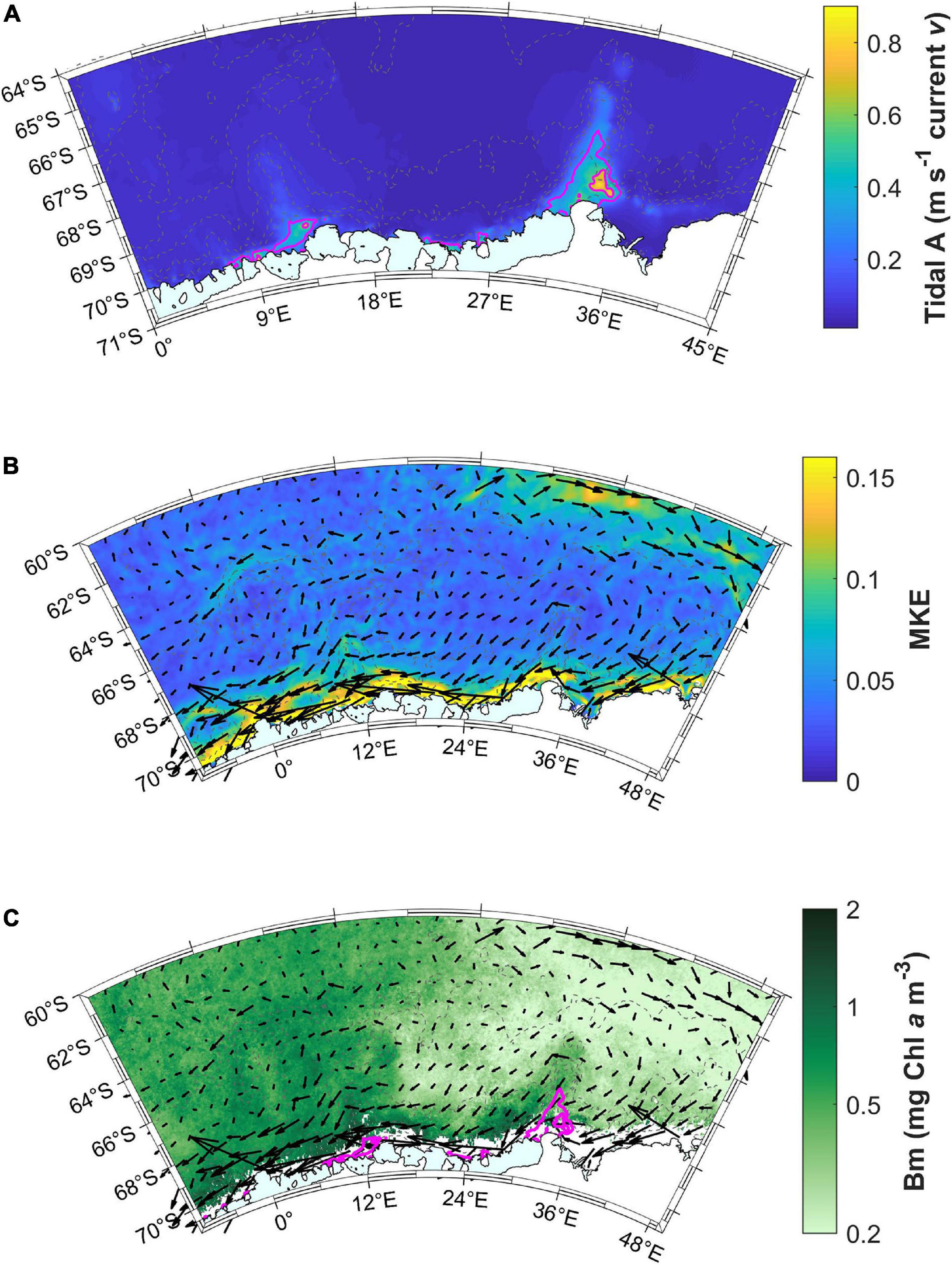
Figure 11. (A) Tidal model results showing the sum of the major axis tidal amplitude (A) in current velocity (v) for the diurnal (Q1, O1, P1, K1) and semi-diurnal (M2, S2, K2) constituents. The magenta lines are 0.3 m s^–1 contours of tidal currents. Note the smaller geographical area compared to the other maps. (B) Mean kinetic energy (MKE) and surface current velocity (relative; black vectors) in the area averaged over December to March. (C) Mean Chl a concentration during the bloom (Bm) together with the tidal amplitude contours (magenta lines) and current velocity vectors (black).

Discussion

Geographical Differences in Bloom Phases and Patterns

During the cruise, we observed phytoplankton blooms in different bloom phases. Phytoplankton biomass differed between the sampling areas, where the highest values (1.1 mg m^–3) were close to the lower range of summer bloom values (1.5 mg m^–3) in the Weddell Gyre (Vernet et al., 2019). Bacterial concentrations were in general similar to other studies reporting 2–4 × 10⁵ cells mL^–1 between January and March 2008 at similar latitudes at the prime meridian (Evans and Brussaard, 2012) and 1.5 × 10⁴ to 1.1 × 10⁶ cells mL^–1 at the Antarctic Peninsula in January (Church et al., 2003; Straza et al., 2010). They were the highest at Astrid Ridge and 6° E transect which may implicate remnants of a bloom as bacterial abundance increases with bloom magnitude (Richert et al., 2019).

Based on the observations, Astrid Ridge and the 6° E transect were characterized as a post-bloom scenario due to low phytoplankton biomass, higher bacterial numbers, and satellite data indicating that this area typically has a strong bloom. Maud Rise had a terminating bloom with a visible export of biomass, i.e., a deep Chl a maximum (60–85 m) below the MLD, and clearly elevated fluorescence signals from the base of the MLD down to 200 m (e.g., the average Chl a value at Maud Rise at 150 m was 0.04 mg m^–3), as well as the lowest surface nutrient concentrations between the areas. The bloom observed at CTD station 53 was also past the peak bloom, based on the relatively low photosystem II fluorescence maximum quantum yields (<0.3; not shown), the sharp Chl a maximum right below the MLD, and microscopy pictures of surface samples that showed chlorotic cells (P. Assmy, personal communication). The surface Chl a concentration was still relatively high for mid-March, above 0.5 mg m^–3, and the underway measurements showed that this bloom covered a larger area west of the station 53. This latter bloom will hereafter be referred to as the open-ocean bloom, and will be studied in more details in a separate study (Moreau et al., in prep.).

The results we obtained at sea are compatible with the results of the satellite-based phenology analysis, with blooms ending earlier in Astrid Ridge than the open-ocean bloom. However, at least in the year the cruise took place, the Astrid Ridge and 6° E transect blooms ended earlier than the Maud Rise bloom. Such level of detail on bloom phenology may not be captured by satellites observing ocean color at the sea surface. Surface Chl a concentration during the cruise was similar at Maud Rise and Astrid Ridge, however, high biomass was observed at depth in Maud Rise, whereas it was low throughout the water column at Astrid Ridge and 6° transect. It should be noted, however, that Astrid Ridge was sampled in mid-March whereas Maud Rise was sampled at the end of March, thus the difference in bloom end timing may have been observable earlier given cloud-free conditions. Similarly, the open ocean bloom was sampled earlier than Maud Rise which may have contributed to differences in bloom phase observations between these areas.

The observed differences in the bloom phase between the sampling areas suggested that geographical differences in bloom patterns exist in the area. The phenology indices indeed showed differences across the study area. Five different bloom regimes emerged, which are made visible in Figure 12 by combining bloom magnitude and timing patterns (see section “Bloom Phenology”). The regimes, with their main characteristics described in parentheses, are: coastal areas west of Gunnerus Ridge affected by the Antarctic Slope Current (1; highest bloom magnitudes, bloom initiation follows sea ice retreat); the open ocean bloom area (2; late bloom with a high magnitude); open ocean areas west of Astrid Ridge including Maud Rise (3; medium to high bloom magnitude, bloom initiation possibly controlled by sea ice cover); open ocean areas east of Astrid Ridge (4; low-magnitude blooms); and the southern ACC (5; long-lasting blooms but with a low magnitude). In the following sections we discuss the environmental control of bloom timing and magnitude across the regions. We do this in a chronological order going from bloom initiation, magnitude to bloom end.

FIGURE 12

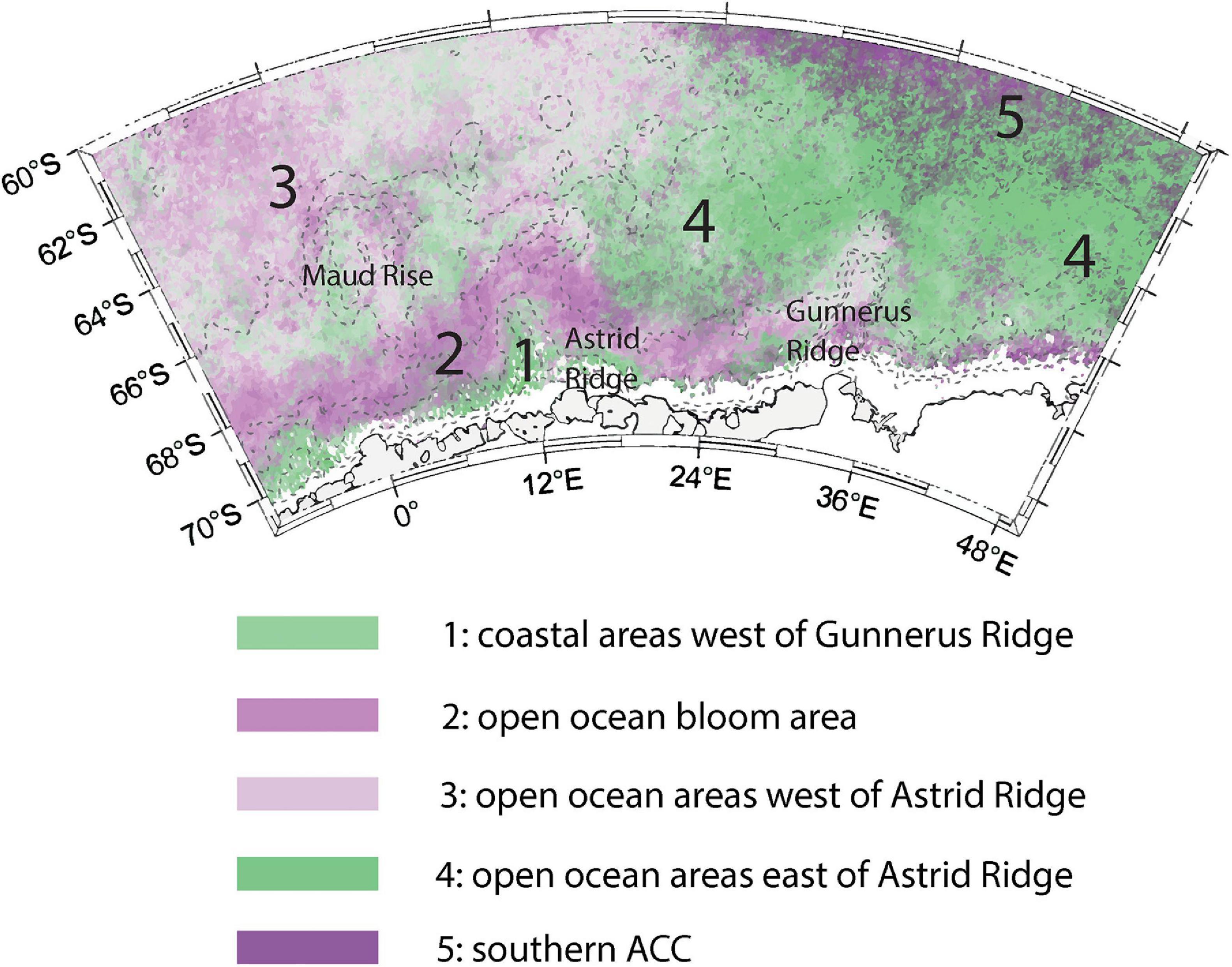
Figure 12. The suggested bloom regimes: 1. coastal areas west of Gunnerus Ridge affected by the Antarctic Slope Current; 2. the open ocean bloom area; 3. open ocean areas west of Astrid Ridge including Maud Rise; 4. open ocean areas east of Astrid Ridge; and 5. the southern ACC.

Bloom Initiation

Bloom initiation in January in the majority of the study area corresponds well with earlier studies of Southern Ocean phytoplankton bloom phenology that included our study area. Thomalla et al. (2011) indicate bloom initiation in December–January for the majority of our study area (their Figure 2) using the same threshold value as in this study (but different pre-analysis of the data). In addition, Soppa et al. (2016), who studied diatom phenology in the Southern Ocean with the help of remote sensing and modeling and used the same threshold value as in this study, showed that bloom initiation mainly takes place in January in our study area (their Figure 3). Finally, the analysis of Ardyna et al. (2017) also suggests bloom initiations in January – February for the bioregions that correspond to our study area, even if using a different processing of the satellite-derived data (i.e., normalized annual bloom cycles and clustering).

It should be noted that the detected bloom initiation may be regarded as the bloom climax if considering the bloom biomass as vertically integrated estimates instead of surface observations, and that the winter (“strict”) onset of the vertically integrated bloom could occur earlier (Llort et al., 2015; see Table 1 and Supplementary Material section 2 for definitions). A recent study concentrating on biogeochemical (BGC) Argo floats providing vertical profile observations every 10-days at Maud Rise, from 2014 to 2019, indeed shows that biomass seemingly increases as early as in November with rapid increases in December (the bloom onset is not marked in their Figure 2), and that bloom climaxes in December–January (von Berg et al., 2020). Further, the detected bloom initiation in this study (i.e., climax) should correspond to favorable environmental conditions (bottom-up control) (Brody et al., 2013; Llort et al., 2015), which are discussed in the next subsections.

Environmental Control: Sea Ice Concentration

In our study, blooms occur after the annual maximum in daily PAR and the summer solstice. ZEu is deeper than MLD during the productive season. Therefore, sufficient incident irradiance, and sufficient light in the water column in open waters (thus where the Chl a-based ZEu was possible to calculate) are available well in advance of the blooms. Light limitation thus likely occurs primarily via sea ice cover, delaying bloom initiation. This effect was studied by separating areas where blooms occur within 3 satellite weeks from sea ice retreat (Figure 9A), as ice edge blooms can be expected to develop within this time (Wright et al., 2010; Perrette et al., 2011; Taylor et al., 2013). Followingly, sea ice cover seems to play an important role for the bloom initiation along the coast and at the ridges, based on the temporal proximity (less than 3 satellite weeks) of sea ice retreat and bloom initiation. The rate of change method indicated that bloom initiation follows sea ice retreat in a somewhat larger area, namely the western – south-western part of the study area (Supplementary Material section 2). Sea ice retreats early in the areas around Maud Rise (de Steur et al., 2007; and Figure 8B). A recent study concentrating on Maud Rise also concludes that sea ice retreat controls the bloom climax timing (von Berg et al., 2020). Whereas other studies using BGC Argo floats show that bloom onset (Arteaga et al., 2020) or growth initiation (approximately corresponding to the bloom onset described here, thus preceding bloom initiation and climax; Hague and Vichi, 2021) can occur well before sea ice retreat (possibly due to unconsolidated ice relieving light limitation; Hague and Vichi, 2021).

Due to the possible delays in detecting bloom initiation with the threshold method (Brody et al., 2013) and due to data gaps (Cole et al., 2012), sea ice could play a role in bloom initiation in a larger area than shown in Figure 9A with areas of bloom initiation within 3 satellite weeks of sea ice retreat. If a 4-week time frame is considered for the sea-ice retreat control on bloom initiation, the majority of the area would be impacted, except for a band around Astrid Ridge (the open-ocean bloom area) and the southern ACC. On the other hand, blooms can develop at sea ice concentration above the retreat threshold of 15% used here (Lancelot et al., 1993; Assmy et al., 2017). Taylor et al. (2013) estimate that blooms in partial sea ice cover and thus not visible for optical satellites contribute significantly (up to 2/3) to the net primary production of the marginal ice zone, and state that sea ice edge blooms start decaying when sea ice disappears completely because of increased wind mixing. In an Arctic, remote sensing-based study, the majority of the pixels (77–89%, depending on the sensor) showed a bloom (defined there as Chl a concentration above 0.5 mg m^–3) within 20 days from sea ice disappearance (i.e., sea ice concentration permanently below 10%) where data was available for this time period, and half of these blooms also terminated within this 20-day period (Perrette et al., 2011). These studies indicate that bloom initiation should follow sea ice retreat closely in time if connected, despite the methodological challenges mentioned here.

The pattern at the coastal areas and the north-eastern part of the study area (southern ACC) is nevertheless robust: bloom initiation follows closely after sea ice retreat in the former and not in the latter. In other words, in the southern ACC conditions are not suitable for phytoplankton blooms when sea ice retreats (despite the ZEu and MLD comparison presented here indicating sufficient light availability), and this area lacks a sea-ice related bloom. Blooms co-located with the ACC have been shown to occur later than could be expected from the seasonal cycle in irradiance and neighboring bio-regions, presumably due to spring light limitation caused by deep mixed layers (Ardyna et al., 2017), except in Scotia Sea where shallow MLDs persist (Prend et al., 2019).

In summary, phytoplankton blooms closely follow the sea ice retreat (within 3 satellite weeks) in coastal areas and in the western part of the study area (the latter based on the rate of change method), which we conclude indicates that bloom initiation is controlled by the length of the sea ice period in these areas.

Environmental Control: Mixed Layer Depth

In our study area, mixed layer is at its deepest latest in October (Pellichero et al., 2017), a time period when ocean color data is not available because of the sea ice cover. Whether this coincides with the bloom onset is thus unclear. The mixed layer is shallowest in December, i.e., shortly before the bloom (Figure 10A), and is already deepening, albeit first with small increments in the study area average, when blooms initiate in January (i.e., bloom initiation based on surface observations). The shallow mixed layer in December could aid the bloom development to initiation/climax by initially concentrating the phytoplankton cells closer to surface and light. MLD is still fairly shallow in January and shallower than ZEu, showing continued favorable light conditions. In the satellite-based phenology study by Thomalla et al. (2011), the maximum Chl a concentrations coincided with the shallowest MLDs (<50 m) over a transect in the Atlantic sector (overlapping with our study area) and based on satellite data and a different MLD product (2° and monthly resolution). Similarly, von Berg et al. (2020) concluded that mixed layer shoaling contributed to the bloom development at Maud Rise (based on BGC-Argo data). The MLD in their data (mainly below 50 m during the blooms) corresponds well with the product we used here. The bloom onset date is not depicted in their Figure 4, but the mixed layer is deepening during the blooms and when biomass is seemingly at its highest level – similar to our observations.

The observed mixed layer deepening during the blooms could further aid bloom development by the dilution effect (fewer encounters with grazers; Behrenfeld, 2010) or by entrainment of new nutrients, counteracting deteriorating light conditions and dilution of phytoplankton biomass. Considering that we lack zooplankton grazing or abundance estimates for the whole seasonal cycle, it is undecided whether the dilution effect caused by the mixed layer deepening can play a role for the bloom initiation, but not for the bloom end as mixed layer is deepening during both events and grazing likely has a role in the control of the bloom end (see section “Bloom End”). In addition, although bloom development during MLD deepening is seemingly similar to the North Atlantic spring bloom (considering, however, the difference between bloom onset and initiation), this happens at a different time of the MLD phenology; following the shallowest spring/summer MLD, as opposed to approaching the winter maximum in the North Atlantic. As blooms happen rather late in the season in our study area because of the sea ice cover and compared to the rest of the Southern Ocean (Ardyna et al., 2017), we can characterize our study area as having summer blooms rather than spring blooms. Indeed, a study based on BGC Argo floats concerning the Southern Ocean (but with very limited float coverage in our study area) suggests that the extremely low light levels under the sea ice prevented the early winter onset of the blooms in the seasonal ice zone, as opposed to the other zones (Arteaga et al., 2020).

Phytoplankton growth enhancement due to entrainment of new nutrients in connection with deepening mixed layer has been suggested in several studies. In the macronutrient-poor subtropical region of the Southern Ocean, nutrient entrainment during mixed layer deepening was considered to be controlling the bloom onset in the winter (Sallée et al., 2015). Wind-induced mixed layer deepening was found to be correlated with elevated Chl a levels in the summer in the Southern Ocean, which was suggested to be due to nutrient entrainment (Carranza and Gille, 2015), further supported by modeling studies (Nicholson et al., 2016). It should, however, be noted that MLD is still relatively shallow when blooms end (the study area MLD average is 37 m in February).

In summary, blooms are observed in the area during moderate mixed layer deepening in January and February. The mixed layer deepening can contribute to growth by entrainment of deep nutrients, including iron. The MLD evolution in relation to the exact bloom onset and the possible role of mixed layer shoaling in November–December for bloom initiation or climax should be studied further.

Bloom Magnitude

The highest bloom magnitude in our study area is linked to bathymetry and ridges in particular (Figures 6C, 11C). High-resolution modeling results showed that the tidal mixing hot spots in the area correspond with high bloom magnitudes, likely due to enhanced upward flux of nutrients and trace metals. The area of high bloom magnitude is, however, larger than the tidal mixing hotspot, thus the enhanced nutrient, and/or tracer metal concentrations are probably transported with the Antarctic Slope Current toward the west. To confirm that these areas have also the highest primary productivity, we obtained the level 4 monthly primary productivity product (based on satellite-derived observations) from Copernicus Marine Services³ and averaged it over the years to get the monthly climatology. The geographical pattern outlined above is confirmed in this dataset (not shown). We thus conclude that tidally induced mixing is a major mechanism in creating higher biomass and primary production along Gunnerus and Astrid Ridges.

The common view of Southern Ocean phytoplankton dynamics is that continental shelves and coasts are areas of enhanced productivity (e.g., Arrigo et al., 2008), but here we see spatial differences within this province, with the coastal areas east of Gunnerus Ridge having a low bloom magnitude. Adjacent to the coastal regime is the open-ocean bloom area, with high biomass. The offshore waters have otherwise lower biomass than the shelf areas. Smith and Comiso (2008) suggested deeper mixed layers of deeper waters as the reason for the lower productivity of the open ocean compared to shelf waters, likely due to the co-limitation of iron and nutrients in a deep mixing state and higher iron requirements at lower irradiances, though this hypothesis has been challenged (Strzepek et al., 2012). MLDs are, however, shallow in most parts of our study area in the productive season. Regarding the pelagic province, the main observation is that the bloom magnitude is higher in the west than the east side of the study area. This west side is part of the Weddell Gyre and corresponds to the eastern part of the Weddell Gyre where currents from the north turn westward, which results in nutrient entrainment from Circumpolar Deep Water and redistribution into the area (the Weddell Gyre characteristics are reviewed in Vernet et al., 2019). Furthermore, the gyre flow pattern fosters upwelling and therefore enhanced nutrient levels.

Within this western area lies the Maud Rise sea mount, with relatively enhanced bloom magnitude surrounding it compared to the other parts of the western area. We also observed during our cruise a strong, though likely terminating, bloom with deep-lying biomass. A study focusing on BGC-Argo floats in the area shows that the Maud Rise blooms have higher biomass than the ones recorded further north in the Weddell Gyre (von Berg et al., 2020). The sea mount topography of Maud Rise and the Taylor column circulation likely contribute to upward (micro)nutrient fluxes (de Steur et al., 2007; Jena and Pillai, 2020; von Berg et al., 2020) enabling enhanced biomass, as suggested also for Pine Bank in the Scotia Sea (Prend et al., 2019).

Coastal polynyas could not be studied in detail because the heavy sea ice conditions during the cruise prevented us from reaching the polynyas for sampling, and because of higher uncertainty in the satellite remote sensing data in these areas. The coastal polynyas are not highly productive regions in our study area (Arrigo and van Dijken, 2003), contrasting with many other parts of the Southern Ocean, although regional variability is high (Arrigo and van Dijken, 2003; Moreau et al., 2019). Regional differences have been attributed to strength of basal melt of the adjacent ice shelf and associated overturning circulation (Dinniman et al., 2020), polynya size (Arrigo and van Dijken, 2003), and water mass distribution (Moreau et al., 2019). Another region that does not seem to be particularly productive is the southern ACC, in the north-eastern corner of the study area, where blooms have a long duration but low magnitude. In fact, Sokolov and Rintoul (2007) found that the ACC mainly enhances productivity in combination with topographic features and associated upwelling, and consequently not in the area described here.

In conclusion, multiple processes and environmental factors seem to control the bloom magnitude in our study area. In particular, the interactions of tides and oceanic currents with bottom topography and the associated water column mixing seem to play a major role in enhancing phytoplankton biomass. It should also be noted that zooplankton grazing likely affects the observed bloom magnitude (see following section “Bloom End”), however, we do not have data to assess this on such large scale.

Bloom End

The bloom end in February results in bloom duration of mainly 2–4 weeks, except for the southern ACC (Figure 7B). Soppa et al. (2016) found a similar duration of blooms in a study concentrating on Southern Ocean diatom blooms. Neither sea ice, light or nutrient conditions seem to determine the bloom end and thus its limited duration, leaving grazing as a suggested controlling factor.

Sea ice does not seem to play a strong role in bloom end, based on the long time-interval (several weeks) between the bloom end and the sea-ice advance (Figure 9B). However, this cannot be excluded in the areas very near to the coast which were not included in the analysis. Sea-ice advance is also variable between the years along the coast (higher standard deviations are observed in this area than elsewhere in the study area; Supplementary Figure 5C), which may imply a larger role in some years. Light availability in general also does not seem to be the main cause for the bloom termination as blooms end mainly during February, i.e., before autumn, and the euphotic layer remains deeper than the mixed layer throughout the productive season (including March).

Nutrient exhaustion is a common contributor to bloom decay by limiting the growth rate. However, during our March cruise, when phytoplankton blooms were recently past the peak phase, the macronutrient concentrations even in the surface waters were well above the half-saturation constant ranges or average reported in literature. Growth rate is half of its maximum at half-saturation constant concentrations, which is considered to indicate nutrient limitation. Observed minima for silicic acid, nitrate and phosphate were 33.0, 20.7, and 1.4 μM, respectively, whereas the half-saturation constants reported for diatoms are up to 22 μM for silicic acid, up to 10.2 μM for nitrate, and on average 1.2 μM (up to 8.9 μM) for phosphate (reviewed in Sarthou et al., 2005). Furthermore, iron addition experiments conducted during the cruise in the southern cruise area showed minimal iron limitation of the phytoplankton communities, as observed through short-term changes in photophysiology (A. Singh, personal communication). Whilst these results only confirm the situation for 1 year as opposed to the long-term satellite data, they seem to indicate that neither macronutrient nor iron limitation terminates phytoplankton blooms in the western part of the study area. For the post-bloom areas such as Astrid ridge, remineralization of nutrients may have happened considering the higher bacterial numbers (thus increasing the nutrients concentrations after the bloom), but even the more active blooms such as at Maud Rise had surface nutrient concentrations exceeding the half-saturation constants, although they were the lowest over the whole cruise area. Another possible process supplying nutrients after the bloom end (thus contradicting the conclusion above) is autumn mixing, but deep winter mixing is needed to fully replenish the iron reservoirs (Tagliabue et al., 2014), which was not the case given the shallow MLDs measured during our cruise.

Another important factor controlling phytoplankton blooms is grazing. Lancelot et al. (1993) observed that protozoan grazing exerted a strong control on an ice-edge phytoplankton bloom in the western Weddell Sea, and was responsible for the decrease in phytoplankton concentration together with physical factors (e.g., dilution due to mixed layer deepening). In addition, an episodic krill passage was able to graze the phytoplankton (from 2.5 to 0.3 mg Chl a m^–3) within hours. On the contrary, macronutrients or trace metals were not observed to play a major role for the bloom magnitude in the study of Lancelot et al. (1993). In addition, other field (Dubischar and Bathmann, 1997; Whitehouse et al., 2009; Hoppe et al., 2017) and modeling studies (Llort et al., 2015; Le Quéré et al., 2016) from the Southern Ocean indicate that grazing controls phytoplankton biomass and bloom decline at least in certain areas. In the Weddell Gyre, for example, microzooplankton grazing is a major controlling factor and more important than larger zooplankton, while viral infections are suggested to be of less importance (reviewed in Vernet et al., 2019). Regarding total losses, a recent study partly concerning our study area and based on bio-optical observations from BGC-Argo floats, concluded that grazing (including viral lysis) was responsible for 83% of the losses on average and was by far more important than phytodetritus sinking (Moreau et al., 2020). In addition, grazing was found to be more important in the later part of the production season.

Sampling and observations of zooplankton and micronekton during the cruise revealed that grazers were present in the autumn, but also showed large regional variations in both abundances and composition. The high concentrations of krill swarms in the vicinity of 6° E transect (yellow – red colors in Figure 5) and, to a lesser extent, Astrid ridge, indicated strong herbivorous grazing of the phytoplankton community. Mesozooplankton abundances and biomass were highest at Maud Rise, however, the zooplankton community composition with high proportions of small copepods and carnivorous zooplankton does not necessary lead to a strong grazing pressure. This together with the absence of krill may indicate a lower grazing pressure on bloom-forming, large phytoplankton in Maud Rise compared to the other stations. However, it is dependent on the phytoplankton community composition, and morphological defenses (e.g., spines), whether grazing from the zooplankton community of this composition was of importance (Smetacek et al., 2004).

Similarly to the bloom initiation discussed earlier, detecting the bloom end from satellite data may suffer from data gaps. Maud Rise phytoplankton blooms ended presumably much later compared to the analysis presented here in the study of von Berg et al. (2020) who used BGC-Argo floats and water column vertical profiles (their Figure 2). The surface satellite observations used here cannot capture deep features such as deep Chl a maxima, which often occur when surface nutrients are being depleted, thus the analysis could artificially indicate early bloom termination. However, deep Chl a maxima can also indicate biomass export to depth rather than an actively growing bloom, when observed below the mixed layer or as a narrow band close to the pycnocline. The bloom we observed at Maud Rise at the end of March was considered to be exporting due to Chl a maxima well below the MLDs and high Chl a values in depth (below 100 m). Finally, the export of phytodetritus observed at Maud Rise could indicate that grazing has a smaller role for the bloom end in this area than elsewhere in the cruise area, which would be consistent with the observed patterns in zooplankton and micronekton abundance as discussed above. Iron limitation could not be excluded as a termination cause for the surface bloom as there were no incubation experiments available from Maud Rise during our campaign. Our sampling was condensed in the relatively isolated and stationary water column on top of Maud Rise (de Steur et al., 2007) where growth conditions may differ from the areas around.

In summary, we hypothesize that top-down control by zooplankton and micronekton contributes strongly to blooms termination in the area, possibly excluding Maud Rise. Grazing may, however, act in concert with other controlling factors. As Behrenfeld and Boss (2018) point out, growth does not have to stop for a bloom to terminate, but to decelerate so that loss rates such as grazing can exceed growth rates. Therefore, at least theoretically, any growth condition that is deteriorating (although still sufficient to enable growth) could also contribute to bloom end. Regarding light availability, although still sufficient, the temporal patterns of deepening of the mixed layer (which circulates algal cells deeper, i.e., to lower light conditions) and the shortening day length mean it is continuously diminishing. In addition, cloudiness increases after the seasonal minimum in the summer, which also decreases light availability (Verlinden et al., 2011).

Methodological Challenges

Remote sensing is inherently less precise than other methods because the measurements are indirect, restricted to the upper ocean and, e.g., in the case of ocean color must be disentangled from atmospheric influence. No other method can, however, offer the long-term dataset with high spatial coverage used here, but it is important to bear in mind some of the caveats. The polar oceans have in addition specific challenges (reviewed in IOCCG, 2015), including low sun angles affecting, e.g., the quality of atmospheric correction, frequent cloud cover (especially along the ice edge) and ice cover. Sun elevation is sufficient at the latitudes described here in the productive season, but both the latter issues result, among other things, in gaps in data, and with regard to sea ice in addition to possible biases in data because of the adjacency effect (Bélanger et al., 2007). To account for the adjacency effect, we excluded data close to the sea ice. Interpolation of the data reduced the gaps but cannot eliminate them. Phytoplankton blooms may in reality start earlier than detected due to (1) challenges related to the bloom definitions, the phenology method used and vertically integrated vs. surface observations (see Supplementary Material section 2), (2) data gaps affecting the threshold value (Cole et al., 2012) or masking parts of the bloom development, and (3) the lack of early observations due to partial sea ice cover. The literature (Taylor et al., 2013; von Berg et al., 2020) and primary productivity product indicate primary production and bloom development already in December, thus it is wise to recognize December as part of the productive season, despite the analysis here showing bloom initiation in January. Likewise, blooms may extend to March. In any case, January–February is the main period for phytoplankton blooms and primary production, particularly January. In addition, against this background, we consider that the shorter duration of the blooms when data are less or not interpolated (Supplementary Figure 2) suggests that the interpolation methods are not creating unrealistic results but rather improve the data quality. Finally, it is also important to bear in mind that variability between years is fairly large, but primarily concerns the exact timing of the bloom which may vary, and less so the bloom duration.

The MLD product from Pellichero et al. (2017) uses a variety of data sources, but unfortunately in our study area the data coverage is somewhat poorer than in other more studied regions (see their Figure 1D), therefore our use of this data product could suffer from local uncertainty. The product corresponds, however, reasonably well with the cruise data and with a recent study using Argo floats (von Berg et al., 2020). Furthermore, errors in satellite Chl a concentration will also affect the estimation of ZEu, because the algorithm is based on satellite-derived Chl a (Morel et al., 2007). Validation studies for remotely sensed Chl a in the Southern Ocean have divergent conclusions ranging from good agreement (Moutier et al., 2019) to underestimation (with overall magnitudes and geographical patterns depending on the algorithm used; Johnson et al., 2013) when using standard algorithms. While the underestimation didn’t affect the results of a phenology study (Sallée et al., 2015) and would also in this study be less of an issue because of, e.g., relative thresholds, it would mean that ZEu is in reality shallower than indicated in the data product. These uncertainties could affect the conclusion that ZEu is always deeper than MLD in the productive season. Note, however, that the critical depth (concerning average light absorbed in mixing conditions) is deeper than ZEu, i.e., the zone where net photosynthesis occurs (compensation depth).

Summary

Based on the presented analyses and the available data, we suggest the following bloom regimes in the study area: coastal areas west of Gunnerus Ridge affected by the Antarctic Slope Current (1); the open ocean bloom area (2); open ocean areas west of Astrid Ridge including Maud Rise (3); open ocean areas east of Astrid Ridge (4); and the southern ACC (5) (Figure 12).

In addition, coastal polynyas and other areas very close to the coast may form their own regime, but had to be excluded from this analysis. To understand the controlling factors of bloom development in these areas, direct sampling, e.g., through tagged seals and field campaigns, is needed.

In the coastal areas and at the ridges the bloom initiation is controlled by sea ice retreat. In the areas west of Gunnerus Ridge, bloom magnitude is enhanced by tidal current interaction with ridge topography.

In the open ocean areas west of Astrid Ridge the bloom initiation is likely controlled by sea ice retreat especially in areas surrounding Maud Rise. The bloom magnitude is enhanced by flow patterns in the Weddell Gyre and current interaction with topography (the latter especially concerning areas around Maud Rise). The open-ocean bloom falls geographically between these two areas, occurs later in the season and shows to have to some extent its own environmental control (S. Moreau, personal communication), that will be studied in a separate paper.

In the open ocean areas east of Astrid Ridge the bloom magnitude is low, resulting at least partly from the absence of upstream topographic features, where interactions with oceanic currents could enhance upward nutrient fluxes. The MLD evolution may play a role for bloom initiation, as sea ice retreat does not seem to play a strong role, although this cannot be fully excluded.

In the Southern ACC, the blooms last longer (more than 4 weeks) but have a low magnitude as the ACC does not interact with major topographic features in this area.

Regarding the end of the bloom (and followingly, the bloom duration), grazing is seemingly the most plausible controlling factor based on the cruise results and literature. Sea ice advance is considerably later than the bloom end in the majority of the area. Although other environmental conditions such as those affecting light availability are not adverse when blooms end, the deteriorating conditions (MLD deepening, day length shortening, increasing cloudiness) could slow down the growth rates (although still enabling growth) and allow loss rates (e.g., grazing) to overcome, resulting in decreasing phytoplankton concentrations. The control of the bloom timing is likely dependent on several factors and their relative importance may vary between years.

It is also important to note that the bloom initiation used here, based on exceeding a threshold value in surface observations, denotes a time of rapid biomass accumulation and may correspond to the bloom climax of a vertically integrated bloom, whereas the bloom onset can occur considerably earlier and have a different environmental control. Lastly, this study shows the complementariness of satellite-based, ship-based (this study) and autonomous profiler observations (related studies). Further research is needed to confirm these hypotheses, especially the role of grazing in connection with MLD evolution. In addition, studying the control of interannual variability especially in the exact timing of the bloom would improve our understanding. This study can function as a basis for understanding the phytoplankton dynamics in the area.

Data Availability Statement

The datasets presented in this study can be found in online repositories in Kauko et al. (2021), Moreau et al. (2021) (Norwegian Polar Data Centre, Norwegian Polar Institute, https://data.npolar.no/dataset/5e510f85-29e1-42c3-89a5-8766f5c5948c, https://data.npolar.no/dataset/28fbddd2-0fb2-41c9-9f42-60146e28617f), and in Chierici and Fransson (2020) (Norwegian Marine Data Centre, https://doi.org/10.21335/NMDC-1503664923). The satellite data are available from the providers described in Section “Materials and Methods.”

Author Contributions

HK conceptualized the study, conducted the main data analysis, and wrote the manuscript draft. SM, HK, TR-K, AS, TH, LS, AF, MC, TF, and EH planned and conducted the field work. SM, HK, TR-K, and AS processed the Chl a samples and AF and MC the nutrient samples. TF was responsible for the zooplankton sampling and analysis. EH processed the acoustics data. TB provided the FlowCam data. HK and AS analyzed the FCM samples under supervision by GB and TT. HK processed the in situ Chl a fluorescence profile and satellite data with the help of TH and SM. TH processed the CTD data from the cruise. QZ conducted the tidal simulations. All authors contributed to the final version.

Funding

The Southern Ocean Ecosystem cruise 2019 with RV Kronprins Haakon was arranged by the Norwegian Polar Institute, with additional financial support from the Norwegian Ministry of Foreign Affairs. This study was partly funded by the Research Council of Norway (RCN) (grant number 288370) and National Research Foundation, South Africa (grant UID 118715) project in the SANOCEAN Norway–South Africa collaboration, and the flagship research program “Ocean acidification and ecosystem effects in Northern waters” at the FRAM – High North Research Centre for Climate and the Environment. QZ acknowledges support from the Norwegian Research Council project Ocean-ice shelf Interaction and channelized Melting in Dronning Maud Land (iMelt, project number: 295075).

Conflict of Interest

The authors declare that the research was conducted in the absence of any commercial or financial relationships that could be construed as a potential conflict of interest.

Acknowledgments

We thank the captain and crew on RV Kronprins Haakon. Thank you also to John Olav Vinge and Nadine Steiger for assistance with water sampling and processing, Elzbieta Anna Petelenz for guiding the FCM laboratory measurements, Violaine Pellichero for sharing the mixed layer depth product, OC-CCI project for the Chl a satellite data product and three reviewers for constructive comments.

Supplementary Material

The Supplementary Material for this article can be found online at: https://www.frontiersin.org/articles/10.3389/fmars.2021.623856/full#supplementary-material

Footnotes

1. ^ www.globcolour.org
2. ^ https://www.esrl.noaa.gov/gmd/grad/solcalc/
3. ^ https://marine.copernicus.eu/

References

Álvarez, E., and López-Urrutia, Á, and Nogueira, E. (2012). Improvement of plankton biovolume estimates derived from image-based automatic sampling devices: application to FlowCAM. J. Plankton Res. 34, 454–469. doi: 10.1093/plankt/fbs017

PubMed Abstract | CrossRef Full Text | Google Scholar

Ardyna, M., Claustre, H., Sallée, J. B., D’Ovidio, F., Gentili, B., van Dijken, G., et al. (2017). Delineating environmental control of phytoplankton biomass and phenology in the Southern Ocean. Geophys. Res. Lett. 44, 5016–5024. doi: 10.1002/2016GL072428

CrossRef Full Text | Google Scholar

Arrigo, K. R., and van Dijken, G. L. (2003). Phytoplankton dynamics within 37 Antarctic coastal polynya systems. J. Geophys. Res. 108:C83271. doi: 10.1029/2002jc001739

CrossRef Full Text | Google Scholar

Arrigo, K. R., van Dijken, G. L., and Bushinsky, S. (2008). Primary production in the Southern Ocean, 1997-2006. J. Geophys. Res. Ocean. 113, 1997–2006. doi: 10.1029/2007JC004551

CrossRef Full Text | Google Scholar

Arteaga, L. A., Boss, E., Behrenfeld, M. J., Westberry, T. K., and Sarmiento, J. L. (2020). Seasonal modulation of phytoplankton biomass in the Southern Ocean. Nat. Commun. 11:5364. doi: 10.1038/s41467-020-19157-19152

CrossRef Full Text | Google Scholar

Assmy, P., Fernández-Méndez, M., Duarte, P., Meyer, A., Randelhoff, A., Mundy, C. J., et al. (2017). Leads in Arctic pack ice enable early phytoplankton blooms below snow-covered sea ice. Sci. Rep. 7:40850. doi: 10.1038/srep40850

PubMed Abstract | CrossRef Full Text | Google Scholar

Atkinson, A., Ward, P., Hunt, B. P. V., Pakhomov, E. A., and Hosie, G. W. (2012). An overview of Southern Ocean zooplankton data: abundance, biomass, feeding and functional relationships. CCAMLR Sci. 19, 171–218.

Google Scholar

Behrenfeld, M. J. (2010). Abandoning Sverdrup’s critical depth hypothesis on phytoplankton blooms. Ecology 91, 977–989.

Google Scholar

Behrenfeld, M. J., and Boss, E. S. (2018). Student’s tutorial on bloom hypotheses in the context of phytoplankton annual cycles. Glob. Chang. Biol. 24, 55–77. doi: 10.1111/gcb.13858

PubMed Abstract | CrossRef Full Text | Google Scholar

Bélanger, S., Ehn, J. K., and Babin, M. (2007). Impact of sea ice on the retrieval of water-leaving reflectance, chlorophyll a concentration and inherent optical properties from satellite ocean color data. Remote Sens. Environ. 111, 51–68. doi: 10.1016/j.rse.2007.03.013

CrossRef Full Text | Google Scholar

Brandt, R. E., Warren, S. G., Worby, A. P., and Grenfell, T. C. (2005). Surface albedo of the Antarctic sea ice zone. J. Clim. 18, 3606–3622. doi: 10.1175/JCLI3489.1

CrossRef Full Text | Google Scholar

Brody, S. R., Lozier, M. S., and Dunne, J. P. (2013). A comparison of methods to determine phytoplankton bloom initiation. J. Geophys. Res. Ocean. 118, 2345–2357. doi: 10.1002/jgrc.20167

CrossRef Full Text | Google Scholar

Brunet, C., Johnsen, G., Lavaud, J., and Roy, S. (2011). “Pigments and photoacclimation processes,” in Phytoplankton Pigments - Characterization, Chemotaxonomy and Applications in Oceanography, eds S. Roy, C. A. LLewellyn, E. S. Egeland, and G. Johnsen (Cambridge: Cambridge University Press), 445–471.

Google Scholar

Carranza, M. M., and Gille, S. T. (2015). Southern Ocean wind-driven entrainment enhances satellite chlorophyll-a through the summer. J. Geophys. Res. Ocean. 120, 304–323. doi: 10.1002/2014JC010203

CrossRef Full Text | Google Scholar

Cavalieri, D. J., Parkinson, C. L., Gloersen, P., and Zwally, H. Z. (1996). Sea Ice Concentrations from Nimbus-7 SMMR and DMSP SSM/I-SSMIS Passive Microwave Data, Version 1. Antarctica, Daily Data for Years 1997–2019. Boulder, CO: NASA National Snow and Ice Data Center Distributed Active Archive Center. doi: 10.5067/8GQ8LZQVL0VL (accessed February 17, 2021).

CrossRef Full Text | Google Scholar

Chierici, M., and Fransson, A. (2020). Nutrient data (nitrate, phosphate and silicate) in the eastern Weddell gyre, Kong Haakon VII Hav, and the coast of Dronning Maud Land in the Atlantic sector of the Southern Ocean in March 2019. Institute of Marine Research. doi: 10.21335/NMDC-1503664923

CrossRef Full Text | Google Scholar

Church, M. J., DeLong, E. F., Ducklow, H. W., Karner, M. B., Preston, C. M., and Karl, D. M. (2003). Abundance and distribution of planktonic Archaea and Bacteria in the waters west of the Antarctic Peninsula. Limnol. Oceanogr. 48, 1893–1902. doi: 10.4319/lo.2003.48.5.1893

CrossRef Full Text | Google Scholar

Cole, H., Henson, S., Martin, A., and Yool, A. (2012). Mind the gap: the impact of missing data on the calculation of phytoplankton phenology metrics. J. Geophys. Res. 117:C08030. doi: 10.1029/2012JC008249

CrossRef Full Text | Google Scholar

Constable, A. J., Nicol, S., and Strutton, P. G. (2003). Southern Ocean productivity in relation to spatial and temporal variation in the physical environment. J. Geophys. Res. 108:8079. doi: 10.1029/2001JC001270

CrossRef Full Text | Google Scholar

de Steur, L., Holland, D. M., Muench, R. D., and Mcphee, M. G. (2007). The warm-water “‘Halo”’ around Maud Rise: properties, dynamics and impact. Deep Sea Res. I 54, 871–896. doi: 10.1016/j.dsr.2007.03.009

CrossRef Full Text | Google Scholar

Dinniman, M. S., St-Laurent, P., Arrigo, K. R., Hofmann, E. E., and van Dijken, G. L. (2020). Analysis of Iron Sources in Antarctic Continental Shelf Waters. J. Geophys. Res. Ocean. 125:e2019JC015736. doi: 10.1029/2019JC015736

CrossRef Full Text | Google Scholar

Dong, J., Speer, K., and Jullion, L. (2016). The Antarctic slope current near 30∘ E. J. Geophys. Res. Ocean. 121, 1051–1062. doi: 10.1038/175238c0

CrossRef Full Text | Google Scholar

Dubischar, C. D., and Bathmann, U. V. (1997). Grazing impact of copeods and salps on phytoplankton in the Atlantic sector of the Southern Ocean. Deep Sea Res. Part II 44, 415–433.

Google Scholar

Egbert, G. D., and Erofeeva, S. Y. (2002). Efficient inverse modeling of barotropic ocean tides. J. Atmos. Ocean. Technol. 19, 183–204.

Google Scholar

Evans, C., and Brussaard, C. P. D. (2012). Regional variation in lytic and lysogenic viral infection in the Southern Ocean and its contribution to biogeochemical cycling. Appl. Environ. Microbiol. 78, 6741–6748. doi: 10.1128/AEM.01388-1312

CrossRef Full Text | Google Scholar

Falahat, S., and Nycander, J. (2015). On the generation of bottom-trapped internal tides. J. Phys. Oceanogr. 45, 526–545. doi: 10.1175/JPO-D-14-0081.1

CrossRef Full Text | Google Scholar

Fer, I., Darelius, E., and Daae, K. B. (2016). Observations of energetic turbulence on the Weddell Sea continental slope. Geophys. Res. Lett. 43, 760–766. doi: 10.1002/2015GL067349

CrossRef Full Text | Google Scholar

Flexas, M. M., Schodlok, M. P., Padman, L., Menemenlis, D., and Orsi, A. H. (2015). Role of tides on the formation of the Antarctic Slope front at the weddell-scotia confluence. J. Geophys. Res. Ocean. 120, 3658–3680. doi: 10.1002/2014JC010372.Received

CrossRef Full Text | Google Scholar

Frouin, R., Franz, B. A., and Werdell, P. J. (2003). “The SeaWiFS PAR product,” in Algorithm Updates for the Fourth SeaWiFS Data Reprocessing, eds S. B. Hooker and E. R. Firestone (Washington, D.C.: NASA), 46–50.

Google Scholar

Grasshoff, K., Kremling, K., and Ehrhardt, M. (2009). Methods of Seawater Analysis, 3th Edn. Hoboken, NJ: Wiley-VCH.

Google Scholar

Grosjean, P., and Denis, K. (2014). “Supervised classification of images, applied to plankton samples using R and Zooimage,” in Data Mining Applications with R, eds Y. Zhao and Y. Cen (Cambridge, MA: Academic Press), 331–365. doi: 10.1016/B978-0-12-411511-8.00013-X

CrossRef Full Text | Google Scholar

Hague, M., and Vichi, M. (2021). Southern Ocean biogeochemical Argo detect under-ice phytoplankton growth before sea ice retreat. Biogeosciences 18, 25–38. doi: 10.5194/bg-18-25-2021

CrossRef Full Text | Google Scholar

Holm-Hansen, O., and Riemann, B. (1978). Chlorophyll a determination: improvements in methodology. Oikos 30, 438–447. doi: 10.2307/3543338

CrossRef Full Text | Google Scholar

Holte, J., and Talley, L. (2009). A new algorithm for finding mixed layer depths with applications to Argo data and Subantarctic mode water formation. J. Atmos. Ocean. Technol. 26, 1920–1939. doi: 10.1175/2009JTECHO543.1

CrossRef Full Text | Google Scholar

Hoppe, C. J. M., Klaas, C., Ossebaar, S., Soppa, M. A., Cheah, W., Laglera, L. M., et al. (2017). Controls of primary production in two phytoplankton blooms in the Antarctic Circumpolar Current. Deep. Res. Part II 138, 63–73. doi: 10.1016/j.dsr2.2015.10.005

PubMed Abstract | CrossRef Full Text | Google Scholar

IOCCG (2015). “Ocean colour remote sensing in polar seas,” in IOCCG Report Series, Vol. 16, eds M. Babin, K. Arrigo, S. Bélanger, and M.-H. Forget (Dartmouth: International Ocean Colour Coordinating Group).

Google Scholar

Jena, B., and Pillai, A. N. (2020). Satellite observations of unprecedented phytoplankton blooms in the Maud Rise polynya, Southern Ocean. Cryosphere 14, 1385–1398. doi: 10.5194/tc-14-1385-2020

CrossRef Full Text | Google Scholar

Johnson, R., Strutton, P. G., Wright, S. W., McMinn, A., and Meiners, K. M. (2013). Three improved satellite chlorophyll algorithms for the Southern Ocean. J. Geophys. Res. Ocean. 118, 3694–3703. doi: 10.1002/jgrc.20270

CrossRef Full Text | Google Scholar

Kauko, H., Moreau, S., and Hattermann, T. (2021). Southern Ocean Ecosystem cruise 2019 Vertical in situ Chlorophyll a Profiles [Data set]. Norwegian Polar Institute. doi: 10.21334/npolar.2021.5e510f85

CrossRef Full Text | Google Scholar

Korneliussen, R. J., Heggelund, Y., Macaulay, G. J., Patel, D., Johnsen, E., and Eliassen, I. K. (2016). Acoustic identification of marine species using a feature library. Methods Oceanogr. 17, 187–205. doi: 10.1016/j.mio.2016.09.002

CrossRef Full Text | Google Scholar

Lancelot, C., Mathot, S., Veth, C., and de Baar, H. (1993). Factors controlling phytoplankton ice-edge blooms in the marginal ice-zone of the northwestern Weddell Sea during sea ice retreat 1988: field observations and mathematical modelling. Polar Biol. 13, 377–387. doi: 10.1007/BF01681979

CrossRef Full Text | Google Scholar

Lannuzel, D., Vancoppenolle, M., van der Merwe, P., de Jong, J., Meiners, K. M., Grotti, M., et al. (2016). Iron in sea ice: review and new insights. Elem. Sci. Anthr. 4:130. doi: 10.12952/journal.elementa.000130

CrossRef Full Text | Google Scholar

Le Paih, N., Hattermann, T., Boebel, O., Kanzow, T., Lüpkes, C., Rohardt, G., et al. (2020). Coherent seasonal acceleration of the Weddell Sea boundary current system driven by upstream winds. J. Geophys. Res. Ocean. 125:e2020JC016316. doi: 10.1029/2020jc016316

CrossRef Full Text | Google Scholar

Le Quéré, C., Buitenhuis, E. T., Moriarty, R., Alvain, S., Aumont, O., Bopp, L., et al. (2016). Role of zooplankton dynamics for Southern Ocean phytoplankton biomass and global biogeochemical cycles. Biogeosciences 13, 4111–4133. doi: 10.5194/bg-13-4111-2016

CrossRef Full Text | Google Scholar

Legendre, L. (1990). The significance of microalgal blooms for fisheries and for the export of particulate organic carbon in oceans. J. Plankton Res. 12, 681–699. doi: 10.1093/plankt/12.4.681

PubMed Abstract | CrossRef Full Text | Google Scholar

Llort, J., Lévy, M., Sallée, J.-B., and Tagliabue, A. (2015). Onset, intensification, and decline of phytoplankton blooms in the Southern Ocean. ICES J. Mar. Sci. 72, 1971–1984.

Google Scholar

Maclennan, D. N., Fernandes, P. G., and Dalen, J. (2002). A consistent approach to definitions and symbols in fisheries acoustics. ICES J. Mar. Sci. 59, 365–369. doi: 10.1006/jmsc.2001.1158

CrossRef Full Text | Google Scholar

Marie, D., Brussaard, C. P. D., Thyrhaug, R., Bratbak, G., and Vaulot, D. (1999). Enumeration of marine viruses in culture and natural samples by flow cytometry. Appl. Environ. Microbiol. 65, 45–52. doi: 10.1128/aem.65.1.45-52.1999

PubMed Abstract | CrossRef Full Text | Google Scholar

Moreau, S., Boyd, P. W., and Strutton, P. G. (2020). Remote assessment of the fate of phytoplankton in the Southern Ocean sea-ice zone. Nat. Commun. 11:3108. doi: 10.1038/s41467-020-16931-16930

CrossRef Full Text | Google Scholar

Moreau, S., Kauko, H., Ryan-Keogh, T., Singh, A., and Bratbak, G. (2021). Southern Ocean Ecosystem cruise 2019 biogeochemistry [Data set]. Norwegian Polar Institute. doi: 10.21334/npolar.2021.28fbddd2

CrossRef Full Text | Google Scholar

Moreau, S., Lannuzel, D., Janssens, J., Arroyo, M. C., Corkill, M., Cougnon, E., et al. (2019). Sea ice meltwater and circumpolar deep water drive contrasting productivity in three Antarctic polynyas. J. Geophys. Res. Ocean. 124, 2943–2968. doi: 10.1029/2019JC015071

CrossRef Full Text | Google Scholar

Morel, A., Huot, Y., Gentili, B., Werdell, P. J., Hooker, S. B., and Franz, B. A. (2007). Examining the consistency of products derived from various ocean color sensors in open ocean (Case 1) waters in the perspective of a multi-sensor approach. Remote Sens. Environ. 111, 69–88. doi: 10.1016/j.rse.2007.03.012

CrossRef Full Text | Google Scholar

Moutier, W., Thomalla, S. J., Bernard, S., Wind, G., Ryan-Keogh, T. J., and Smith, M. E. (2019). Evaluation of chlorophyll-a and POC MODIS Aqua products in the Southern Ocean. Remote Sens. 11:1793. doi: 10.3390/rs11151793

CrossRef Full Text | Google Scholar

Naughten, K. A., Meissner, K. J., Galton-Fenzi, B. K., England, M. H., Timmermann, R., Hellmer, H. H., et al. (2018). Intercomparison of Antarctic ice-shelf, ocean, and sea-ice interactions simulated by MetROMS-iceshelf and FESOM 1.4. Geosci. Model Dev. 11, 1257–1292. doi: 10.5194/gmd-11-1257-2018

CrossRef Full Text | Google Scholar

Nicholson, S. A., Lévy, M., Llort, J., Swart, S., and Monteiro, P. M. S. (2016). Investigation into the impact of storms on sustaining summer primary productivity in the Sub-Antarctic Ocean. Geophys. Res. Lett. 43, 9192–9199. doi: 10.1002/2016GL069973

CrossRef Full Text | Google Scholar

Nicolaus, M., Gerland, S., Hudson, S. R., Hanson, S., Haapala, J., and Perovich, D. K. (2010). Seasonality of spectral albedo and transmittance as observed in the Arctic Transpolar Drift in 2007. J. Geophys. Res. Ocean. 115:C11011. doi: 10.1029/2009JC006074

CrossRef Full Text | Google Scholar

Orsi, A. H., Whitworth, T., and Nowlin, W. D. (1995). On the meridional extent and fronts of the Antarctic Circumpolar current. Deep. Res. Part I 42, 641–673. doi: 10.1016/0967-0637(95)00021-W

CrossRef Full Text | Google Scholar

Padman, L., Erofeeva, S. Y., and Flicker, H. A. (2008). Improving Antarctic tide models by assimilation of ICESat laser altimetry over ice shelves. Geophys. Res. Lett. 35:L22504. doi: 10.1029/2008GL035592

CrossRef Full Text | Google Scholar

Padman, L., Fricker, H. A., Coleman, R., Howard, S., and Erofeeva, L. (2002). A new tide model for the Antarctic ice shelves and seas. Ann. Glaciol. 34, 247–254. doi: 10.3189/172756402781817752

CrossRef Full Text | Google Scholar

Pawlowicz, R. (2020). M_Map: A Mapping Package for MATLAB. Available online at: www.eoas.ubc.ca/rich/map.html (accessed November 19, 2019).

Google Scholar

Pellichero, V., Sallée, J.-B., Schmidtko, S., Roquet, F., and Charrassin, J.-B. (2017). The ocean mixed layer under Southern Ocean sea-ice: seasonal cycle and forcing. J. Geophys. Res. Ocean. 122, 1608–1633. doi: 10.1002/2016JC011970

CrossRef Full Text | Google Scholar

Pereira, A. F., Beckmann, A., and Hellmer, H. H. (2002). Tidal mixing in the Southern Weddell Sea: results from a three-dimensional model. J. Phys. Oceanogr. 32, 2151–2170.

Google Scholar

Perovich, D. K., and Polashenski, C. (2012). Albedo evolution of seasonal Arctic sea ice. Geophys. Res. Lett. 39:L08501. doi: 10.1029/2012GL051432

CrossRef Full Text | Google Scholar

Perrette, M., Yool, A., Quartly, G. D., and Popova, E. E. (2011). Near-ubiquity of ice-edge blooms in the Arctic. Biogeosciences 8, 515–524. doi: 10.5194/bg-8-515-2011

CrossRef Full Text | Google Scholar

Prend, C. J., Gille, S. T., Talley, L. D., Mitchell, B. G., Rosso, I., and Mazloff, M. R. (2019). Physical drivers of phytoplankton bloom initiation in the Southern Ocean’s Scotia Sea. J. Geophys. Res. Ocean. 124, 5811–5826. doi: 10.1029/2019JC015162

CrossRef Full Text | Google Scholar

Racault, M.-F., Le Quéré, C., Buitenhuis, E., Sathyendranath, S., and Platt, T. (2012). Phytoplankton phenology in the global ocean. Ecol. Indic. 14, 152–163. doi: 10.1016/j.ecolind.2011.07.010

CrossRef Full Text | Google Scholar

Richert, I., Yager, P. L., Dinasquet, J., Logares, R., Riemann, L., Wendeberg, A., et al. (2019). Summer comes to the Southern Ocean: how phytoplankton shape bacterioplankton communities far into the deep dark sea. Ecosphere 10:e02641. doi: 10.1002/ecs2.2641

CrossRef Full Text | Google Scholar

Sallée, J.-B., Llort, J., Tagliabue, A., and Lévy, M. (2015). Characterization of distinct bloom phenology regimes in the Southern Ocean. ICES J. Mar. Sci. 72, 1985–1998.

Google Scholar

Sarthou, G., Timmermans, K. R., Blain, S., and Tréguer, P. (2005). Growth physiology and fate of diatoms in the ocean: a review. J. Sea Res. 53, 25–42. doi: 10.1016/j.seares.2004.01.007

CrossRef Full Text | Google Scholar

Sathyendranath, S., Brewin, R. J. W., Brockmann, C., Brotas, V., Calton, B., Chuprin, A., et al. (2019). An ocean-colour time series for use in climate studies: the experience of the ocean-colour climate change initiative (OC-CCI). Sensors 19:4285. doi: 10.3390/s19194285

PubMed Abstract | CrossRef Full Text | Google Scholar

Sathyendranath, S., Jackson, T., Brockmann, C., Brotas, V., Calton, B., Chuprin, A., et al. (2020). ESA Ocean Colour Climate Change Initiative (Ocean_Colour_cci): Global chlorophyll-a data Products Gridded on a Sinusoidal Projection, Version 4.2. Centre for Environmental Data Analysis. Available online at: https://catalogue.ceda.ac.uk/uuid/99348189bd33459cbd597a58c30d8d10 (accessed September 15, 2020).

Google Scholar

Sieracki, C. K., Sieracki, M. E., and Yentsch, C. S. (1998). An imaging-in-flow system for automated analysis of marine microplankton. Mar. Ecol. Prog. Ser. 168, 285–296. doi: 10.3354/meps168285

CrossRef Full Text | Google Scholar

Skarðhamar, J., and Skagseth, Ø, and Albretsen, J. (2015). Diurnal tides on the Barents Sea continental slope. Deep. Res. Part I 97, 40–51. doi: 10.1016/j.dsr.2014.11.008

CrossRef Full Text | Google Scholar

Smetacek, V., Assmy, P., and Henjes, J. (2004). The role of grazing in structuring Southern Ocean pelagic ecosystems and biogeochemical cycles. Antarct. Sci. 16, 541–558. doi: 10.1017/S0954102004002317

CrossRef Full Text | Google Scholar

Smetacek, V., Klaas, C., Strass, V. H., Assmy, P., Montresor, M., Cisewski, B., et al. (2012). Deep carbon export from a Southern Ocean iron-fertilized diatom bloom. Nature 487, 313–319. doi: 10.1038/nature11229

PubMed Abstract | CrossRef Full Text | Google Scholar

Smith, W. O. Jr., and Comiso, J. C. (2008). Influence of sea ice on primary production in the Southern Ocean: a satellite perspective. J. Geophys. Res. 113:C05S93. doi: 10.1029/2007JC004251

CrossRef Full Text | Google Scholar

Sokolov, S., and Rintoul, S. R. (2007). On the relationship between fronts of the Antarctic Circumpolar Current and surface chlorophyll concentrations in the Southern Ocean. J. Geophys. Res. 112:C07030. doi: 10.1029/2006JC004072

CrossRef Full Text | Google Scholar

Soppa, M. A., Völker, C., and Bracher, A. (2016). Diatom phenology in the Southern Ocean: mean patterns, trends and the role of climate oscillations. Remote Sens. 8:420. doi: 10.3390/rs8050420

CrossRef Full Text | Google Scholar

Søreide, J. E., Leu, E., Berge, J., Graeve, M., and Falk-Petersen, S. (2010). Timing of blooms, algal food quality and Calanus glacialis reproduction and growth in a changing Arctic. Glob. Chang. Biol. 16, 3154–3163. doi: 10.1111/j.1365-2486.2010.02175.x

CrossRef Full Text | Google Scholar

Stammerjohn, S. E., Martinson, D. G., Smith, R. C., and Iannuzzi, R. A. (2008). Sea ice in the western Antarctic Peninsula region: spatio-temporal variability from ecological and climate change perspectives. Deep Sea Res. II 55, 2041–2058. doi: 10.1016/j.dsr2.2008.04.026

CrossRef Full Text | Google Scholar

Stewart, A. L., Klocker, A., and Menemenlis, D. (2019). Acceleration and overturning of the Antarctic Slope current by winds, eddies, and tides. J. Phys. Oceanogr. 49, 2043–2074. doi: 10.1175/JPO-D-18-0221.1

CrossRef Full Text | Google Scholar

Straza, T. R. A., Ducklow, H. W., Murray, A. E., and Kirchman, D. L. (2010). Abundance and single-cell activity of bacterial groups in Antarctic coastal waters. Limnol. Oceanogr. 55, 2526–2536. doi: 10.4319/lo.2010.55.6.2526

CrossRef Full Text | Google Scholar

Strzepek, R. F., Hunter, K. A., Frew, R. D., Harrison, P. J., and Boyd, P. W. (2012). Iron-light interactions differ in Southern Ocean phytoplankton. Limnol. Oceanogr. 57, 1182–1200. doi: 10.4319/lo.2012.57.4.1182

CrossRef Full Text | Google Scholar

Sun, S., Hattermann, T., Pattyn, F., Nicholls, K. W., Drews, R., and Berger, S. (2019). Topographic shelf waves control seasonal melting near Antarctic ice shelf grounding lines. Geophys. Res. Lett. 46, 9824–9832. doi: 10.1029/2019GL083881

CrossRef Full Text | Google Scholar

Svensen, C., Halvorsen, E., Vernet, M., Franzè, G., Dmoch, K., Lavrentyev, P. J., et al. (2019). Zooplankton communities associated with new and regenerated primary production in the Atlantic inflow north of Svalbard. Front. Mar. Sci. 6:293. doi: 10.3389/fmars.2019.00293

CrossRef Full Text | Google Scholar

Tagliabue, A., Bowie, A. R., Boyd, P. W., Buck, K. N., Johnson, K. S., and Saito, M. A. (2017). The integral role of iron in ocean biogeochemistry. Nature 543, 51–59. doi: 10.1038/nature21058

PubMed Abstract | CrossRef Full Text | Google Scholar

Tagliabue, A., Sallée, J., Bowie, A. R., Lévy, M., Swart, S., and Boyd, P. W. (2014). Surface-water iron supplies in the Southern Ocean sustained by deep winter mixing. Nat. Geosci. 7, 314–320. doi: 10.1038/NGEO2101

CrossRef Full Text | Google Scholar

Taylor, M. H., Losch, M., and Bracher, A. (2013). On the drivers of phytoplankton blooms in the Antarctic marginal ice zone: a modeling approach. J. Geophys. Res. 118, 63–75. doi: 10.1029/2012JC008418

CrossRef Full Text | Google Scholar

Thomalla, S. J., Fauchereau, N., Swart, S., and Monteiro, P. M. S. (2011). Regional scale characteristics of the seasonal cycle of chlorophyll in the Southern Ocean. Biogeosci. Dis. 8, 2849–2866. doi: 10.5194/bg-8-2849-2011

CrossRef Full Text | Google Scholar

Thyng, K. M., Greene, C. A., Hetland, R. D., Zimmerle, H. M., and DiMarco, S. F. (2016). True colors of oceanography: guidelines for effective and accurate colormap selection. Oceanography 29, 9–13. doi: 10.5670/oceanog.2016.66

CrossRef Full Text | Google Scholar

Verlinden, K. L., Thompson, D. W. J., and Stephens, G. L. (2011). The three-dimensional distribution of clouds over the Southern Hemisphere high latitudes. J. Clim. 24, 5799–5811. doi: 10.1175/2011JCLI3922.1

CrossRef Full Text | Google Scholar

Vernet, M., Geibert, W., Hoppema, M., Brown, P. J., Haas, C., Hellmer, H. H., et al. (2019). The Weddell Gyre, Southern Ocean: present knowledge and future challenges. Rev. Geophys. 57, 623–708. doi: 10.1029/2018RG000604

CrossRef Full Text | Google Scholar

von Berg, L., Prend, C. J., Campbell, E. C., Mazloff, M. R., Talley, L. D., and Gille, S. T. (2020). Weddell Sea phytoplankton blooms modulated by sea ice variability and polynya formation. Geophys. Res. Lett. 47:e2020GL087954. doi: 10.1029/2020GL087954

CrossRef Full Text | Google Scholar

Vu, M. T. T., Jepsen, P. M., and Hansen, B. W. (2014). A comprehensive and precise quantification of the calanoid copepod Acartia tonsa (Dana) for intensive live feed cultures using an automated zooimage system. Aquaculture 42, 225–231. doi: 10.1016/j.aquaculture.2013.12.002

CrossRef Full Text | Google Scholar

Whitehouse, M. J., Atkinson, A., Ward, P., Korb, R. E., Rothery, P., and Fielding, S. (2009). Role of krill versus bottom-up factors in controlling phytoplankton biomass in the northern Antarctic waters of South Georgia. Mar. Ecol. Prog. Ser. 393, 69–82. doi: 10.3354/meps08288

CrossRef Full Text | Google Scholar

Wright, S. W., van den Enden, R. L., Pearce, I., Davidson, A. T., Scott, F. J., and Westwood, K. J. (2010). Phytoplankton community structure and stocks in the Southern Ocean (30-80∘E) determined by CHEMTAX analysis of HPLC pigment signatures. Deep. Res. Part II Top. Stud. Oceanogr. 57, 758–778. doi: 10.1016/j.dsr2.2009.06.015

CrossRef Full Text | Google Scholar

Xing, X., Claustre, H., Blain, S., D’Ortenzio, F., Antoine, D., Ras, J., et al. (2012). Quenching correction for in vivo chlorophyll fluorescence acquired by autonomous platforms: a case study with instrumented elephant seals in the Kerguelen region (Southern Ocean). Limnol. Oceanogr. Methods 10, 483–495. doi: 10.4319/lom.2012.10.483

CrossRef Full Text | Google Scholar

Zhou, Q., and Hattermann, T. (2020). Modeling ice shelf cavities in the unstructured-grid, finite volume community Ocean model: implementation and effects of resolving small-scale topography. Ocean Model. 146:101536. doi: 10.1016/j.ocemod.2019.101536

CrossRef Full Text | Google Scholar