 Alexei I. Pinchuk
 Sonia D. Batten
 Wesley W. Strasburger3
- 1Department of Fisheries, College of Fisheries and Ocean Sciences, University of Alaska, Juneau, AK, United States
- 2North Pacific Marine Science Organization, Nanaimo, BC, Canada
- 3Ted Stevens Marine Research Institute, National Oceanic and Atmospheric Administration, Juneau, AK, United States
The eastern North Pacific experienced a prolonged heat wave in 2014–2016 manifested by high sea surface temperature anomalies in the south-central Gulf of Alaska (GOA). The event provided a natural experiment on the response of the southern GOA ecosystem to a dramatic change in sea temperature. Spatial and temporal variability in zooplankton communities following the culmination of the heat wave was investigated as a part of the NOAA Eastern GOA Ecosystem Assessment program in 2016–2017. Here, for the first time in the GOA, we report consistent observations of doliolid (Dolioletta tritonis) swarms observed in the upper mixed layer beyond the shelf break during both years, with the maximal density of 3,847 ind m–3 recorded in August 2016 and coinciding with the location of an offshore cyclonic mesoscale eddy. Doliolid density was significantly lower on the shelf. The long-term Continuous Plankton Recorder (CPR) data indicated that doliolid blooms in the south-central GOA may have occurred in the past two decades during El-Nino events. Coincidentally, doliolids prevailed in the diets of juvenile sablefish collected along the eastern coast of GOA both during the 2014–2016 heat wave and during 1997–1998 El Nino. Thus, we speculate that warming trends may increase the importance of doliolids in the GOA pelagic food web.
Introduction
Ecological impacts of climate change have become increasingly apparent affecting the organizational hierarchy of species and communities with marine ecosystems (Walther et al., 2002). In the recent decade, there has been an apparent rise in the frequency and persistence of marine heat waves (Oliver et al., 2018). The ecosystem impacts of these climate events can be severe resulting in shifts in geographical distributions and seasonal cycles and production of marine organisms, adversely affecting human activities (Uye, 2008; Purcell, 2012; Mills et al., 2015). Such extreme events can be viewed as climate change “stress-tests,” providing insight into possible changes in ecosystem structure, species’ abundance and distribution, and the frequency and strength of ecosystem disruptions. In order to maintain resilient and sustainable marine ecosystems, it is imperative that management and conservation strategies are developed to mitigate and/or adapt to these impacts.
The North Pacific undergoes periodic influences of warmer periods typically resulting from large scale teleconnections of El Nino events. The 2014–2015 period was marked by unusually high sea level pressure which resulted in reduced wind mixing and advection and led to high near surface sea temperature anomalies in the south-central Gulf of Alaska (GOA) (termed “the warm blob”) (Bond et al., 2015). The heat wave peaked in 2016 coinciding with the strong 2015–2016 El Niño (Newman et al., 2018; Walsh et al., 2018). After a brief cooling in 2017, temperatures increased again during 2018–2019, suggesting a prolonged climate event rather than a discrete heatwave (Litzow et al., 2020). The phenomenon attracted considerable attention as a potential future scenario for the changing climate. It has been speculated that the persistent elevated water temperatures may result in dramatic shifts in latitudinal distribution of marine organisms and structural reorganization of food webs along the North American Pacific coast, thus influencing commercial fisheries and impacting coastal communities. For example, warm temperatures in combination with other stressors have resulted in increase of abundance and production rates of gelatinous organisms such as hydrozoan and scyphozoan medusae, and pyrosomes (Purcell, 2012; Brodeur et al., 2019), and in decrease of commercially important fish such as Pacific Cod (Gadus macrocephalus) (Barbeaux et al., 2019).
The southeastern GOA coastal and bottom topography is defined by the Fairweather-Queen Charlotte fault system which forms the boundary between the convergent North American and Pacific tectonic plates (Brothers et al., 2018). The Queen Charlotte fault lies underwater in close vicinity to the narrow (5–10 km) continental shelf with depths<300 m and steep continental slope (Weingartner et al., 2009). The northern part of the boundary zone is adjacent to the submerged Yakutat Terrane which extends the shelf zone to ∼50 km offshore. The basin and continental slope circulation are dominated by a diffuse, weak eastern boundary Alaska Current with mean speeds of ∼5 cm s–1 and a width of several hundred kilometers (Weingartner et al., 2009; Figure 1). The Alaska Current diverges from the east-flowing North Pacific Current offshore from British Columbia and carries relatively warm and saline waters into the higher latitudes of the northern GOA. In contrast, the GOA shelf is characterized by a less saline, buoyancy driven Alaska Coastal Current flowing westward within 20–50 km of the shore (Royer, 1982; Weingartner et al., 2005). Mesoscale eddies are often generated along the eastern GOA continental slope leading to substantial exchange between the shelf and the basin, resulting in transport of heat, nutrients, microelements, and organisms across the slope which increase local productivity (Okkonen et al., 2003; Crawford et al., 2007; Ladd et al., 2007; Coyle et al., 2012).
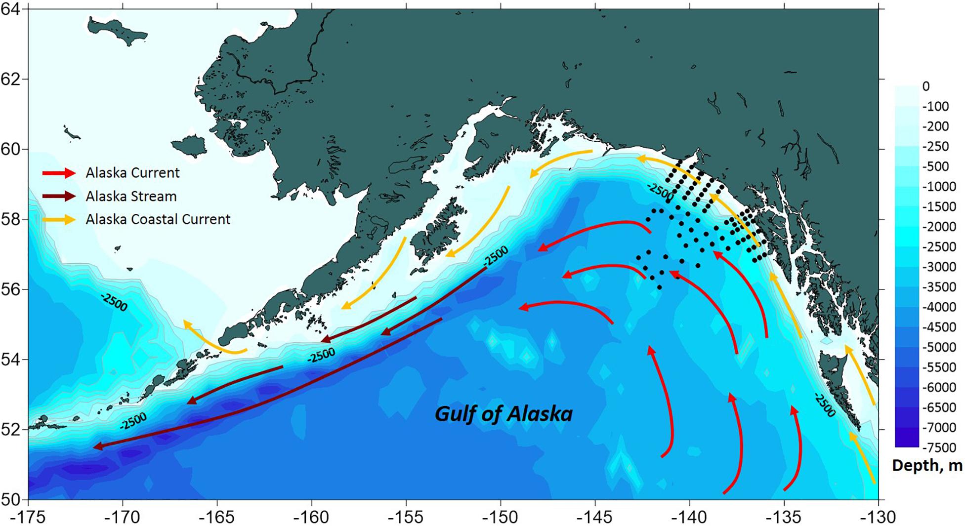
Figure 1. A schematic diagram of oceanic circulation in the Gulf of Alaska. Black dots indicate survey sampling stations.
Doliolids are planktonic tunicates with a complex life cycle, which includes polymorphic asexual zooid stages (called oozooids, trophozooids, and phorozooids) alternating with sexual solitary gonozooids (Deibel, 1998). The high asexual reproduction rate in combination with relatively short generation time governed primarily by temperature and food concentration facilitates rapid population growth under favorable conditions and often results in dense (thousands m–3) swarms of gonozooids typically restricted to the mixed layer above the pycnocline (Paffenhofer and Gibson, 1999; Deibel and Lowen, 2012; Takahashi et al., 2015). Doliolids are filter feeders capable of ingesting a wide size range of food particles including microbes, packaging them into large fecal pellets and thus contributing to vertical carbon flux and a shunt of the microbial loop (Deibel and Paffenhofer, 2009). Their high individual feeding and excretion rates combined with explosive population growth may result in considerable impact on biogeochemical processes in the areas where the blooms occur. Doliolids seem to be adapted to event-scale fluctuations in the environment as opposed to seasonal-scale changes (Deibel and Lowen, 2012). The blooms are often associated with mesoscale physical events such as mid-shelf thermohaline fronts (Atkinson et al., 1978), eddies spinning off a strong boundary current and propagating along the adjacent shelf (Deibel and Paffenhofer, 2009), or meanders and filaments formed by convergent currents with contrasting physical properties (Takahashi et al., 2015). Such intrusions tend to bring nutrients into the euphotic zone fostering high rates of phytoplankton production, which, in turn, can be quickly exploited by doliolids (Paffenhofer and Lee, 1987; Deibel and Paffenhofer, 2009). The patchy and sporadic nature of such events makes doliolid blooms a challenging topic to study.
The sibling species Dolioletta tritonis (Herdman 1888) and Dolioletta gegenbauri (Uljanin 1884) occur in tropical and temperate waters of the Atlantic, Pacific, and Indian oceans and often penetrate as far north as the Faroe Islands following the warm summer transgression (Godeaux, 2003). However, until recently, dense aggregations were found only within the warmer tropical and subtropical core of their biogeographical range (Mackas et al., 1991; Deibel and Paffenhofer, 2009; Takahashi et al., 2015). In this paper, we report the first observation of intense D. tritonis bloom in the southeastern GOA during the 2016–2017 heat wave and utilize long-term data sets and historical data to link doliolid emergence in the southeastern GOA to climate variability.
Materials and Methods
Net Sampling
Samples were collected during NOAA Eastern GOA Ecosystem Assessment surveys in summer 2016 and 2017 (Figure 1). Sampling within the US Exclusive Economic Zone (EEZ) was done along 10 main parallel transects run perpendicular to the coast and supplemental stations spaced 10 to 18–37 km apart. An additional rectangular sampling grid consisted of offshore stations spaced 37 km apart. The nearshore surveys were conducted between July 4 and 28 followed by the offshore sampling continued from August 4 through 10. A total of 72 stations were sampled each year.
Conductivity-temperature-depth (CTD) measurements were taken with a Sea-Bird Electronics Inc. (SBE) 911 or SBE 25 CTD at each station to determine vertical temperature and conductivity profiles. Casts did not exceed 200 m (if bottom depths were>200 m) and were limited to the upper 50 m while sampling the offshore grid.
Seawater samples were collected at five depths (0, 10, 20, 40, and 50 m) to determine total chlorophyll-a (chl-a) concentrations (using Whatman GF/F filters). Filters were stored at –70°C and analyzed with a Turner Designs (TD-700) laboratory fluorometer (Parsons et al., 1984). In situ fluorometric data were calibrated with discrete chl-asamples to estimate chl-a concentrations (r2 = 0.678). The satellite image [Visible Infrared Imaging Radiometer Suite(VIIRS) on the Suomi-NPP] of the northern GOA in June 2016 was obtained from https://earthobservatory.nasa.gov/images/88238/bloom-in-the-gulf-of-alaska. No clear satellite images of the study area were available for the summer 2017 because of extensive cloudiness.
Doliolids were sampled with a 60 cm MARMAP-style bongo frame with a 505 μm mesh net. The net frame was equipped with an SBE 49 CTD transmitting real time tow data. Oblique tows from within 5–10 m off the bottom or from 200 m (at depths>200 m) to the surface were conducted primarily during daylight hours. Only the upper 50 m layer was sampled at the additional offshore grid. Volume filtered was measured with calibrated General Oceanics flowmeters mounted inside the net. All samples were preserved in 5% formalin, buffered with seawater for later processing. In the laboratory, the samples were split with a Folsom splitter and the subsamples were examined to identify and count doliolids. Collections from 2016 were sorted at the Polish Plankton Sorting and Identification Center (Szczecin, Poland) following NOAA protocols which omit identification of doliolid stages and mass (e.g., Eisner et al., 2018). Collections from 2017 were sorted at the University of Alaska (College of Fisheries and Ocean Sciences) in Juneau, AK, United States. Wet mass of doliolids were determined for 2017 samples. Blotted preserved wet mass was measured on a Cahn Electrobalance or Mettler top-loading balance, depending on the size of the doliolids. The wet mass was converted to carbon (C) content using 0.0072 coefficient established for Tunicata (Kiørboe, 2013). The data were uploaded to a Microsoft Access database, and analyses were performed using STATISTICA 6 and R software (R Core Team, 2015).
Continuous Plankton Recorder Sampling
The continuous plankton recorder (CPR) was towed behind commercial ships across the Gulf of Alaska on routes from Alaska to the North American West Coast, from March through October each year, and from the West Coast towards Asia year-around, from 2000 to 2017. Several vessels conducted the sampling over the time series but in each case the CPR was towed in the wake of the ship at a depth of about 7 m.
The details on CPR sampling are provided elsewhere (Batten et al., 2003, 2018). Briefly, water and associated plankton entered the front of the CPR through a small square aperture (1.27 cm2), and then through silk filtering mesh (with a mesh size of 270 μm) which retained the plankton and allowed the water to exit at the back of the machine. The movement of the CPR through the water turned an external propeller which, via a drive shaft and gearbox, moved the filtering mesh across the tunnel at a rate of approximately 10 cm per 18.5 km of tow. As the filtering mesh left the tunnel it was covered by a second band of mesh so that the plankton were sandwiched between these two layers. The mesh layers were then wound into a storage chamber containing buffered 40% formaldehyde preservative (which diluted in the seawater to a concentration of about 4%, sufficient to fix and preserve the plankton).
The towed mesh was processed according to standard CPR protocols (Batten et al., 2003, 2018). It was first cut into separate samples (each representing 18.5 km of tow and about 3 m3 of seawater filtered) and every 4th sample was randomly apportioned amongst the analysts for plankton identification and counting. The ship’s log was used to determine the mid-point latitude and longitude of each sample along with the date and time.
Data Analysis
The stations were split into two groups: (1) the shelf group with<300 m depth and (2) the offshore group with >300 m depth. Since the shelf slope is narrow and steep in the study area, the majority of the offshore stations were located at >1,000 m depths. Depth of the thermocline was computed for each station by locating the depth where dT/dz was maximum (T = temperature, °C; z = depth, m). The mean water-column temperatures above and below the pycnocline, as well as throughout the upper 50 m water column were then computed.
Since only the upper 50 m were sampled on the deep offshore stations, doliolid abundances estimated from other stations were adjusted by proportion of the total volume filtered in the upper 50 m based on the assumption that doliolid aggregations typically occur at shallower depths near the thermocline (e.g.,Paffenhofer et al., 1991; Takahashi et al., 2015). Because of uneven spatial distribution of doliolids, both abundance and directly measured biomass data were fourth-root power transformed to stabilize the variance and reduce heteroscedasticity. Analysis of variance (ANOVA) was used to test for significant effects of location and year on physical and biological variables, and the distribution of residuals was analyzed to ensure it meets the normality assumption. Interpolation of physical and biological values over the sampling area was done on non-transformed data using kriging subroutines in SURFER 12 (Golden Software).
Station-based doliolid abundance data were used to examine how D. tritonis responded to biophysical environmental factors during summer in 2016–2017. Generalized Additive Models (GAMs; Hastie and Tibshirani, 1990; Wood, 2006) were then used to identify significant relationships between doliolid abundance and water properties that had significant effects on doliolid distribution:
where g is a log link, μ is the expectation of observations, s is a smoothing function, ε is an error term, and k1–k4 are the numbers of knots for smoothing functions. We used bottom depth, and the mean temperature, salinity, and non-fractioned chl-a concentration integrated through the upper 50 m at sampling locations. GAMs were run using the mgcv library in R, version 3.2.0 (R Core Team, 2015), with a quasi-Poisson family and cubic regression splines as the smoothing function of predictor variables. A subset of predictor variables that produced the best-fit models was selected using generalized cross validation (GCV) methods (Wood, 2006). Significance of the predictor variables was assessed by using Chi-square statistics calculated by R (R Core Team, 2015). In addition, partial regression plots showing the additive effect of each predictor variable on the doliolid abundance were examined for linearity, significance, and positive and negative effect. Residuals from best-fit models were checked for the assumption of independence and identical distributions. The resulting best-fit model were used to determine which predictor variables may have a significant effect on the doliolid abundance.
The time series of monthly average Pacific Decadal Oscillation (PDO) index anomalies available from the Joint Institute for the Study of the Atmosphere and Ocean1 was used to define cold and warm phases on the Gulf of Alaska during the past two decades. We divided the years into positive, negative, or neutral using 0.5 or –0.5 annual mean PDO values from March through October as the determining values (Table 1). The time series of monthly Ocean Nino index (ONI) was obtained from the National Climate Prediction Center.2
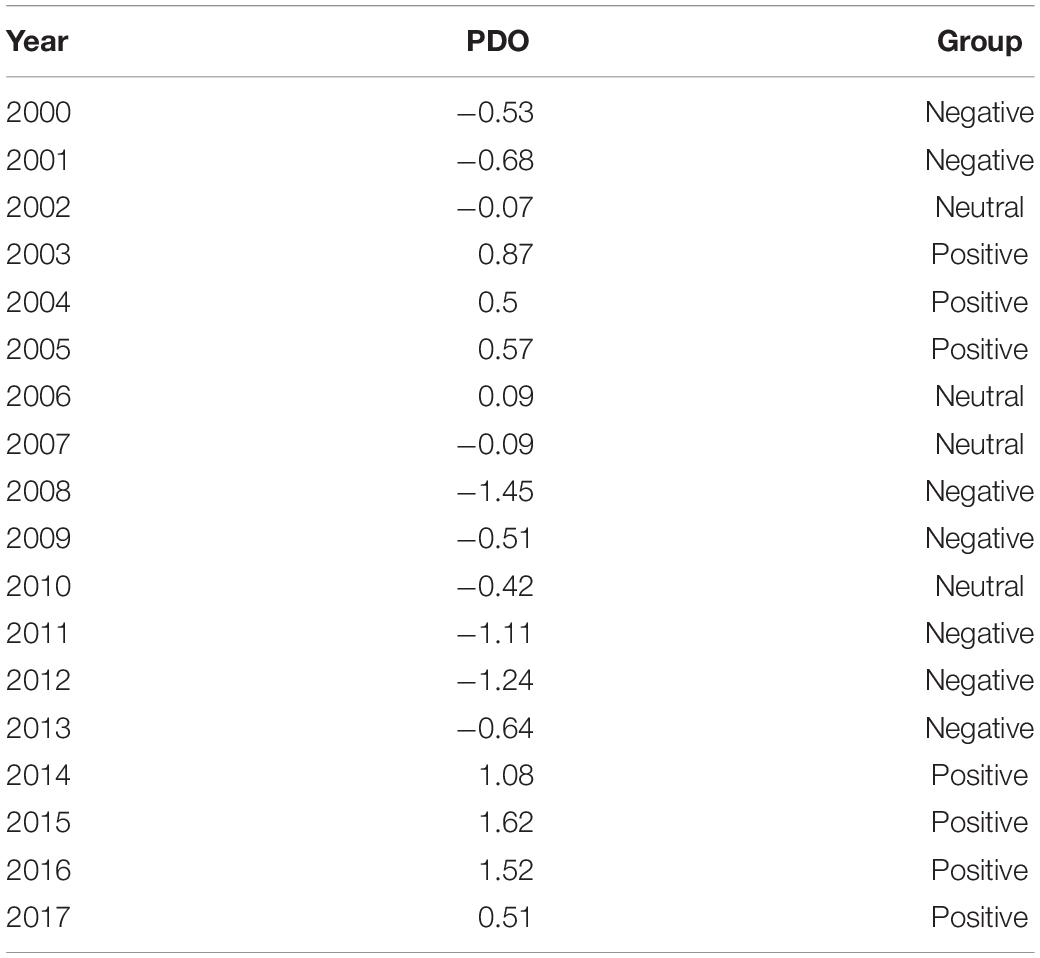
Table 1. Groups of positive, neutral and negative PDO years.
Results
In both 2016 and 2017, a two-layered water column structure marked by a pycnocline located at ∼15 m depth was observed throughout the study area (Figure 2 and Table 2). The upper mixed layer was ∼4°C warmer than the underlying stratum. While mean temperature below the pycnocline did not change significantly between years or regions, the upper layer was ∼1.5°C warmer in 2016 than in 2017 (ANOVA, F = 70.8, p < 0.0001). On average, the entire upper 50 m layer over the slope and basin was ∼1°C warmer in 2016 than in 2017 (ANOVA, F = 44.7, p < 0.0001), while no interannual difference was found on the shelf. The warm core was located offshore beyond the shelf break during both years (Figure 3). While offshore salinity did not differ between the years, a brackish riverine plume was observed during both years in vicinity of Alsek River, spreading along the coast and significantly lowering salinity above the pycnocline by 1.5 PSU (ANOVA, F = 18.8, p < 0.0001). Similar to temperature, mean chl-a concentration was also significantly higher offshore in 2016 than in 2017 (ANOVA, F = 7.4, p < 0.01). A VIIRS satellite image taken three weeks before the 2016 cruise revealed a mesoscale anti-cyclonic eddy ∼400 km offshore in the study area marked by elevated chlorophyll concentrations at the eddy periphery (Figure 4) indicating higher primary production and likely better feeding conditions for zooplankton grazers in 2016.
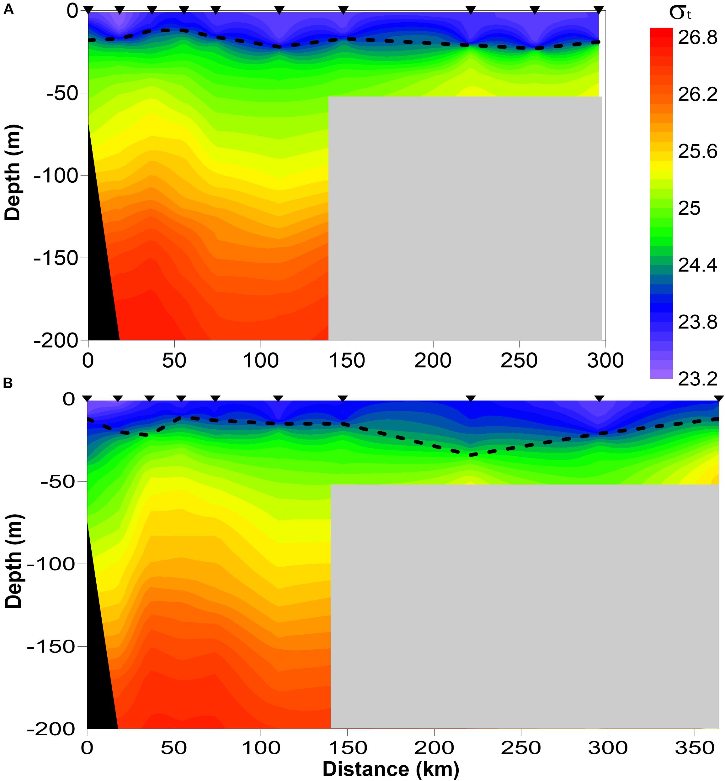
Figure 2. Vertical density (σt) profiles showing pycnocline depth (dashed line) across the study area. (A) 2016, (B) 2017.
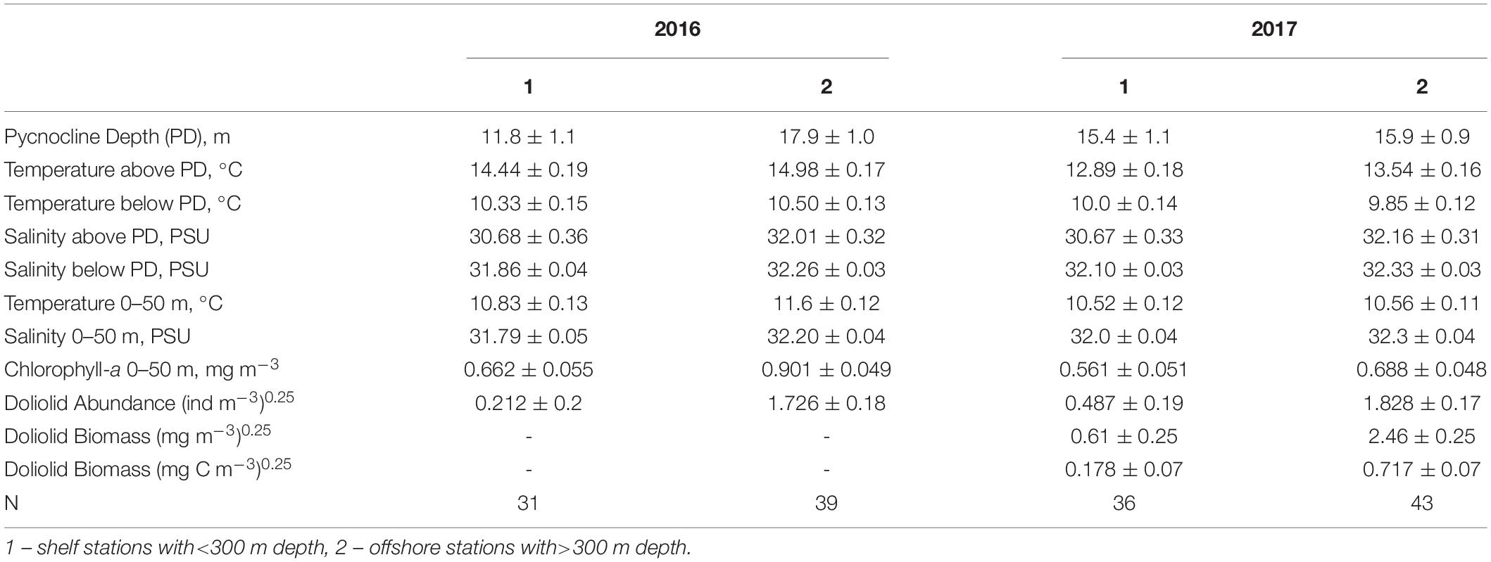
Table 2. Mean (±Standard Error) water properties of the 0–50 m layer observed during zooplankton surveys on the shelf and offshore in the southeastern Gulf of Alaska in 2016 and 2017.
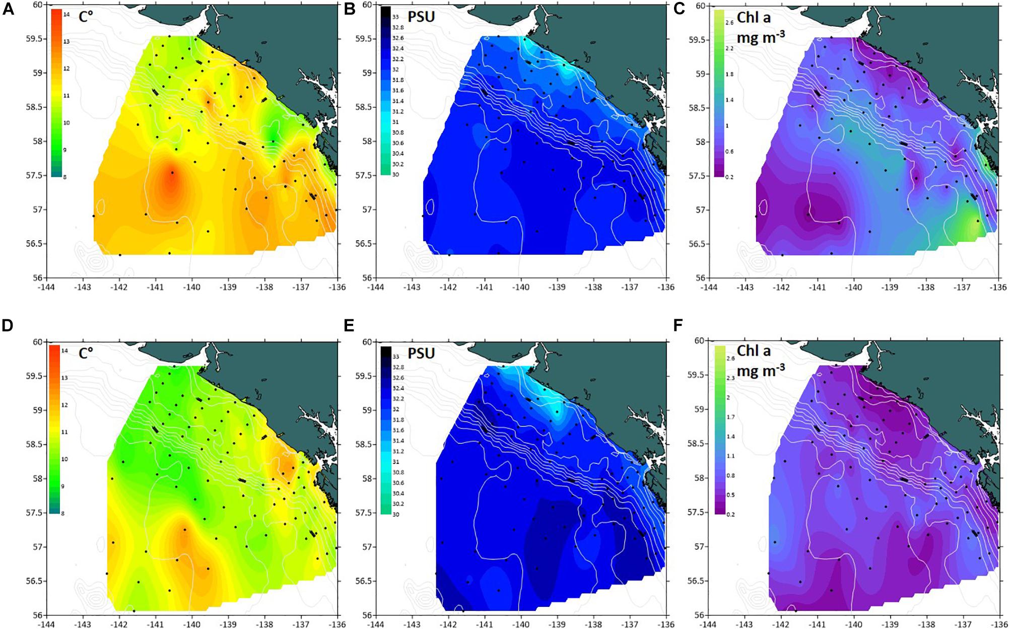
Figure 3. Spatial distribution of biophysical properties in the southeastern Gulf of Alaska in summer 2016–2017. (A,B) mean temperature (°C), (C,D) mean salinity (PSU), (E,F) mean chl-a concentration (mg m− 3) in 0–50 m layer.
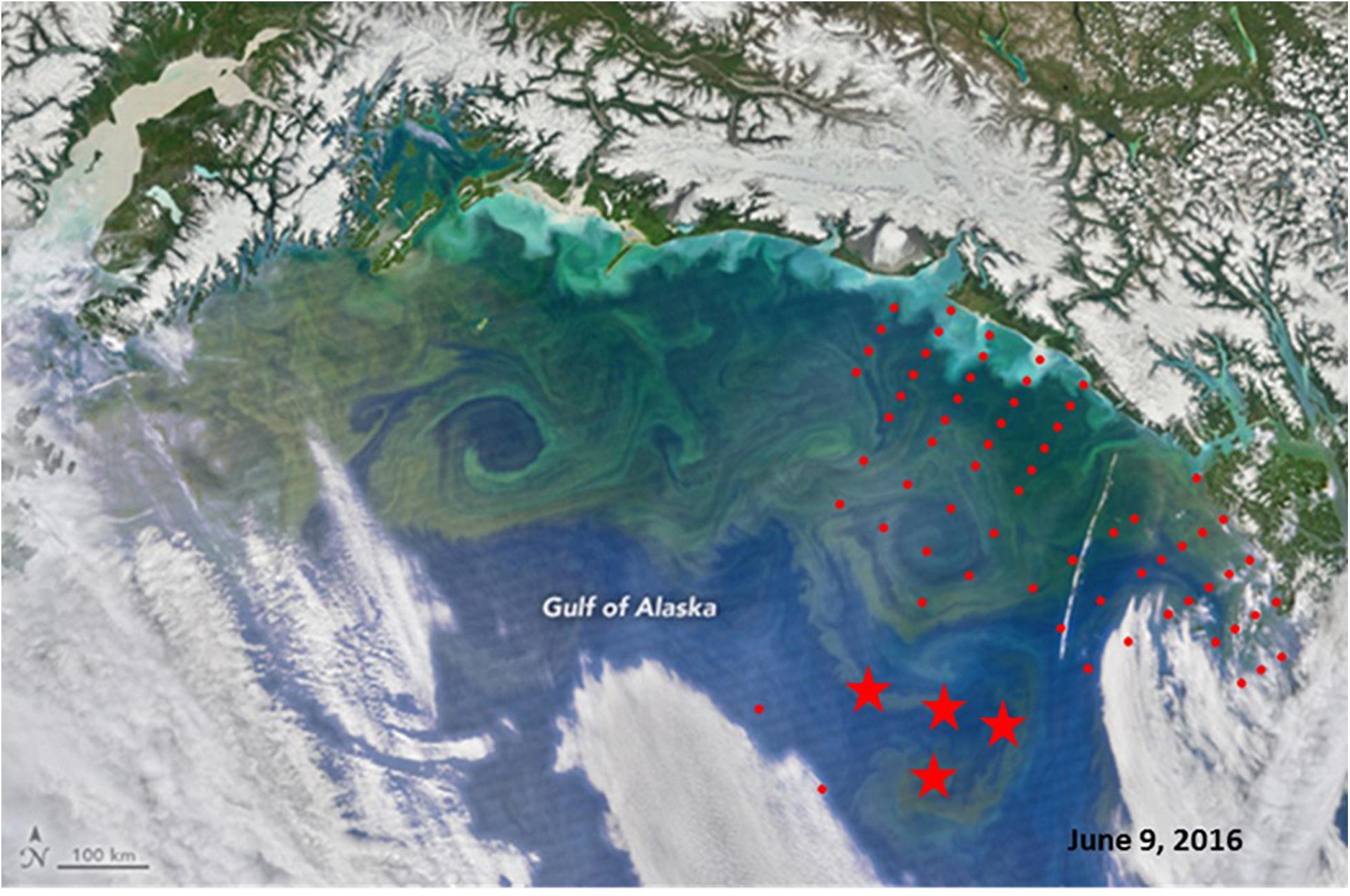
Figure 4. Satellite image of the Northern Gulf of Alaska (VIIRS) obtained on June, 09, 2016 (from https://earthobservatory.nasa.gov/images/88238/bloom-in- the-gulf-of-alaska). Stations from 2016 survey are superimposed (red circles), stars indicate locations of doliolid blooms (>100 ind m− 3).
Dolioletta tritonis were significantly more abundant at offshore stations in the basin than over the shelf (ANOVA, F = 60.3, p < 0.0001) (Table 2). No significant interannual differences in doliolid abundance were observed within each station group. Dense (∼100–800 ind m–3) aggregations of doliolids were observed well beyond the shelf break at deep offshore stations (>3,000 m) in both years (Figure 5). The maximum abundance of 3,847 ind m–3was recorded in 2016 coinciding with the position of the offshore eddy observed a month earlier. In 2017, doliolid biomass was significantly higher offshore than over the shelf (Table 2), ranging from 0.02 to 2,429 mg m–3(0.14–17,489 μg C m–3) offshore and from 0 to 260 mg m–3(0–1,872 μg C m–3) over the shelf. While doliolid developmental stages were not identified in 2016, gonozooids were the most abundant zooid stage in 2017 making up 93.5% of the population with the rest being nurse stages ranging from 1.5 to 20 mm in total length. Our relatively coarse nets probably severely undersampled smaller zooids making analysis of generation distribution patterns impossible. The mean individual gonozooid wet mass at stations, where the bloom was developed in 2017, was 4.15 ± 0.64(SE) mg. This value corresponds to 6.6 mm total length calculated using the length-mass regression for D. tritonis gonozooids from the western subarctic Pacific (Nakamura et al., 2017). This size corresponds to 36.43 μg C according to the length-C mass relationship obtained for laboratory-reared D. gegenbauri gonozooids (Gibson and Paffenhofer, 2000).
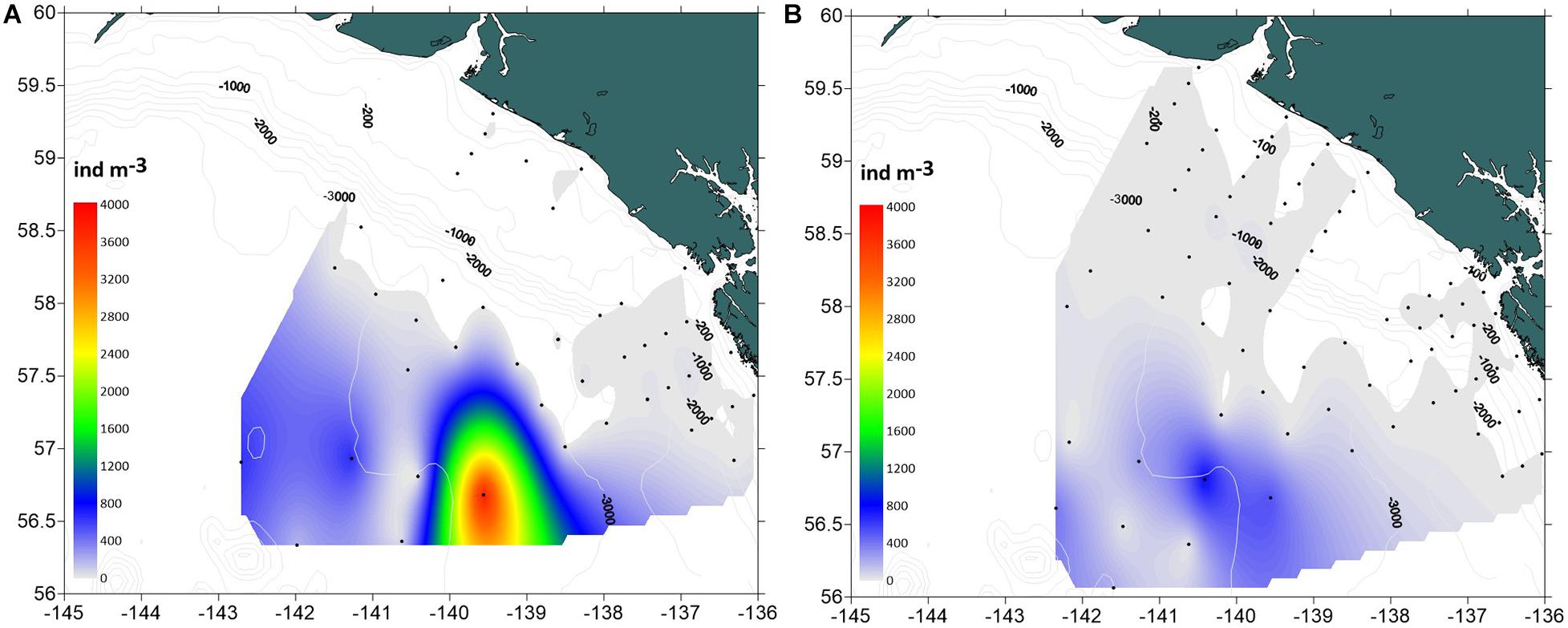
Figure 5. Spatial distribution of Dolioletta tritonis abundance (ind m− 3) in the southeastern Gulf of Alaska in summer 2016–2017. (A) 2016, (B) 2017.
The GAM model with four predictor variables explained 58.5% of the deviance in doliolid abundance. Depth (F = 5.7, p < 0.001), salinity (F = 2.4, p < 0.001), and chl-a (F = 0.925, p < 0.01) had non-linear effects, while temperature did not have any significant effect on doliolid abundance (Figure 6). Abundance sharply increased with depths increasing to 1,000 m and it showed another increase at stations over 3,000 m depth. Salinity had positive effect on abundance when it had exceeded 31.25. The effect of chl-a on doliolid abundance was negative when chl-a concentration exceeded ∼0.7 mg m–3.
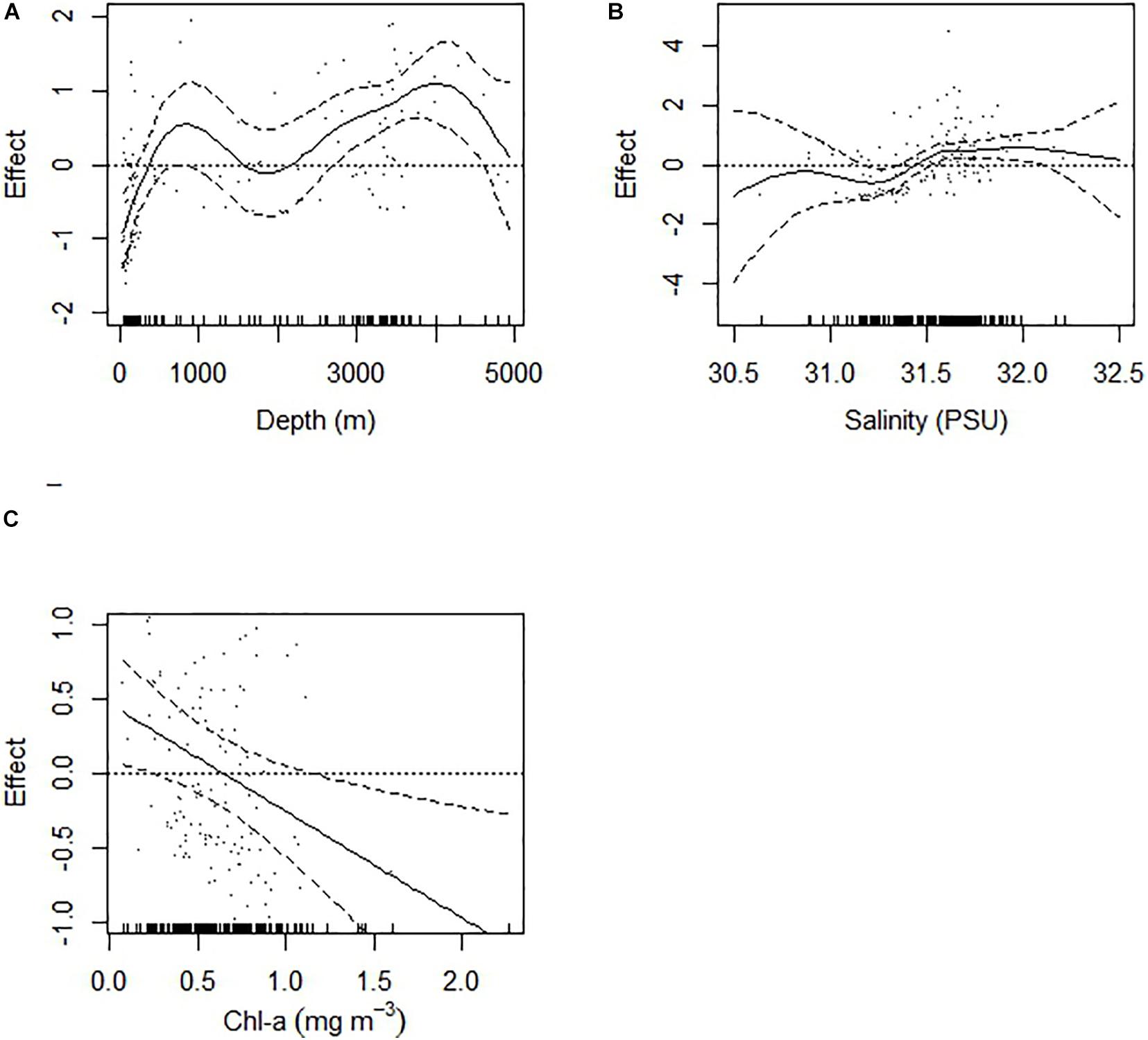
Figure 6. The effects of predictor variables from the GAM on Dolioletta tritonis abundance (ind m− 3). The dashed line represents the 95% confidence interval of the effects. (A) depth (m), (B) salinity, (C) chlorophyll-a (mg m− 3).
The CPR surveys covered a two-decade period with contrasting “warm” vs “cold” stanzas in the North Pacific highly correlated to El-Nino events (Figure 7). The interannual changes in doliolid abundance in the GOA during 2000–2017 showed a distinctive pattern apparently related to climate variability (Figure 8). During strong positive PDO years, doliolids were substantially more abundant and they occurred in deep waters in both the eastern and western GOA. In contrast, doliolids were absent from CPR samples during negative PDO years. During neutral PDO years, doliolids appeared to be restricted to the southeastern GOA where they occurred in moderate quantities.
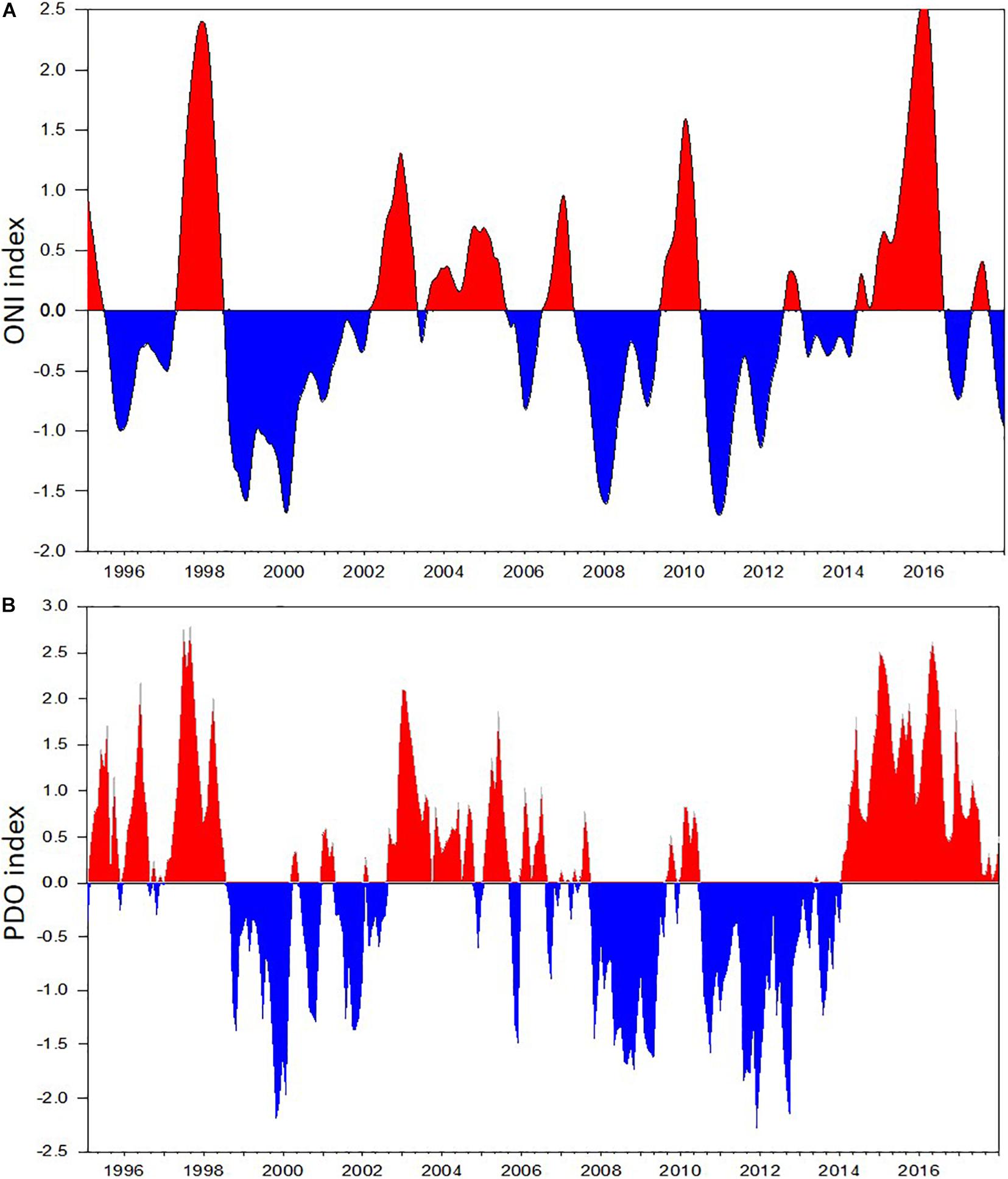
Figure 7. Climate indices based on sea surface temperature measurements in the Pacific Ocean in 1995–2017: (A) Monthly Ocean Nino (ONI) index, (B) Pacific Decadal Oscillation (PDO) index.
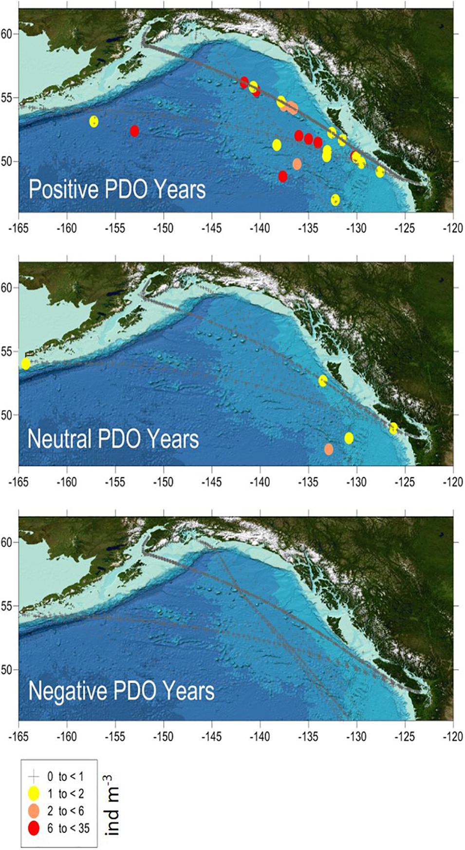
Figure 8. Doliolid abundance (ind m− 3) in the Gulf of Alaska in March–October 2000–2017 based on CPR data. PDO positive years were 2003–2005 and 2014–2017, PDO neutral years were 2002, 2006–2007, and 2010 and PDO negative years were 2000–2001, 2008–2009, and 2011–2013.
In addition, Tunicata [reported as “Ascidia sp. (tunicate)” [sic] and “Salpa sp. (pelagic salp)” [sic]] contributed up to 60% by weight to overall juvenile sablefish (Anoplopoma fimbria) stomach contents collected in the northern GOA during a strong 1997–1998 El-Nino, while during other years they were virtually absent from the diets (Sigler et al., 2001; Figure 9). Juvenile sablefish are pelagic predators and feed almost exclusively near the surface and in the upper layers (e.g.,Brodeur and Pearcy, 1992). Therefore, it is plausible that the reported “Ascidia sp.”, a distinctly sessile organisms morphologically somewhat resembling doliolids, were misidentified, and the report in fact refers to doliolids. Since the contribution of salps to total fish prey weight on average was<1% (Sigler et al., 2001), the increase of tunicates in the sablefish diets during El-Nino years was probably facilitated by doliolids.
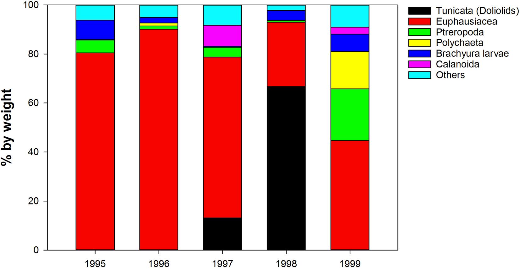
Figure 9. Interannual variability in diet composition (% by weight) of 0-age sable fish in the Gulf of Alaska (from Sigler et al., 2001, modified).
Discussion
For the first time in the southeastern GOA, we recorded dense (>100 ind m–3) doliolid aggregations during summer 2016–2017, typically classified as “blooms” in other world regions (Crocker et al., 1991; Paffenhofer, 2013; Takahashi et al., 2015). The aggregations occurred at offshore stations influenced by the saline Alaska Current which connects the GOA to southern regions of the Pacific Ocean. Since the Alaska Current originates from the lower latitude (35–50°N) North Pacific Current, it appears that the source population of D. tritonis is located within the northern reaches of the North Pacific subtropical gyre and the seed organisms are advected into the GOA. Observations from the US Northeast Pacific GLOBEC program (Weingartner et al., 2002) indicated that doliolids regularly occurred, albeit in extremely low numbers (<0.05 ind m–3), in the northern GOA on the outermost stations along the Seward Line since 1997 (Pinchuk, unpublished), which implies that the Alaska Current is the major conduit for doliolid dispersal along the Alaskan shelf. In contrast, few doliolids were found closer to the shore suggesting limited shoreward advection and/or unfavorable environment on the shelf affected by the low salinity, run-off driven Alaska Coastal Current.
The high abundance of doliolids offshore, where mean chl-a concentration was higher in both years, indicates strong dependence of the thaliacean bloom on phytoplankton availability. Doliolids can feed efficiently on a large variety of prey from<5 μm bacteria to>100 μm diatoms (Crocker et al., 1991), allowing them to take advantage of intense diatom blooms typically occurring during spring and summer in the GOA. While large diatom spring blooms on the GOA shelf are triggered by the onset of thermal stratification starting in wind-protected fjord systems in March and extending over the shelf through April and May (Strom et al., 2001, 2006), summer blooms are often associated with mesoscale eddies which propagate along the shelf edge and bring iron-rich coastal water offshore (Coyle et al., 2012, 2019; Aguilar-Islas et al., 2016). The relatively slow eddy propagation speed (1.5–4 km day–1) and their extended longevity (6–24 months) (Okkonen et al., 2001, 2003) provide persistent conditions for a doliolid population to develop. The physical interactions between propagating eddies and adjacent water masses in the northern GOA are similar to those observed along the North American Atlantic coast (Okkonen et al., 2003). Studies in the South Atlantic Bight indicated that doliolid blooms on the broad continental shelf during summer are associated with formation of mesoscale eddies spinning off the Gulf Stream at the shelf break, and their consequential propagation along the shelf (Deibel and Paffenhofer, 2009). However, in contrast to the GOA, the Gulf Stream eddies bring nutrients from the offshore onto the shallow shelf and foster high rates of phytoplankton production, resulting in favorable feeding environment for doliolids nearshore (Paffenhofer and Lee, 1987; Deibel and Paffenhofer, 2009).
Despite the doliolid’s apparent preference to the offshore water rich in phytoplankton, the GAM showed negative effect of high chl-a concentration on the doliolid abundance. Similarly, the location of dense doliolid patches closely coincided with areas of low chl-a concentration in the Oyashio-Kuroshio region (Nakamura, 1998; Takahashi et al., 2015). This is not surprising considering the high filtration ability of doliolids. Laboratory studies showed that D. gegenbauri gonozooid clearance rates measured at phytoplankton concentrations ranging from 20 to 160 μg C L–1 were similar depending mainly on temperature and individual size, and that a gonozooid of 6.5 mm total length (=35 μg C weight) incubated at 16.5°C cleared approximately 275 mL of seawater per day ingesting ∼15 μg C L–1(Gibson and Paffenhofer, 2000) (see their Figures 5, 6). With the exception of one station in 2016, phytoplankton concentrations in our study area never exceeded 100 μg C L–1, assuming C mg:Chl-a mg ratio of 51 (Lomas et al., 2012). Thus, assuming the same laboratory-derived constant feeding rate for D. tritonis and applying Q10 = 3 (Haskell et al., 1999) to correct for the mean 14.25°C observed in 2016–2017, the aggregated gonozooids at ∼3,000 ind m–3 can sweep clear their resident water volume in ∼47 h ingesting 0.045 g C m–3 day–1. Similarly, less dense aggregations of doliolids in the Oyashio-Kuroshio transitional region cleared their residential volume in ∼10 days (Ishak et al., 2020). While no direct measurements of primary productivity were obtained during our cruises, model simulations run for 2000–2013 using the Regional Ocean Modeling System (ROMS) with an embedded nutrient-phytoplankton-zooplankton (NPZ) estimated late summer (September–October) mean primary production at 30.5 g C m–2 in the upper 30 m layer for the offshore region “P5” from the Canadian boundary to 147°W (Coyle et al., 2019), which converts to a daily value of 0.0169 g C m–3 day–1. Therefore, dense aggregations of doliolids can successfully control primary production in the southeast GOA.
At 20°C, it would take ∼20 days for a newly released D. gegenbauri gonozooid to grow to that size (6.5 mm total length or 35 μg C weight) (Deibel, 1982). Using this rate and applying the same assumptions, the minimal longevity of the D. tritonis bloom in the GOA can be estimated at ∼35 days. The presence of old nurse stages in 2017 also indicate intensive asexual reproduction which must have been persisting for a considerable period. Thus, doliolid blooms in the Gulf of Alaska can substantially impact pelagic food web by quickly reducing local resources available for other planktonic grazers such as copepods and euphausiids.
Gelatinous zooplankton have been considered a trophic cul-de-sac (Dubischar et al., 2012) due to high water content and low nutritional value per unit of volume (Verity and Smetacek, 1996; Sommer et al., 2002). However, recent studies suggest that gelatinous zooplankton has been underestimated as food (Cardona et al., 2012; González Carman et al., 2014). For instance, generally low protein and lipid weight-specific content (∼5% each, e.g.,Dubischar et al., 2006) in Thaliaceans may be compensated by their relatively large body size and high density (Arai, 1986; Larson, 1986), which also make them more visible to visual predators. In addition, Thaliacean passive mobility requires comparably little effort from pelagic predators to consume large quantities (Arai, 1988). Juvenile sablefish (Anoplopoma fimbria), a commercially important species, have been documented consuming Thaliaceans in large proportions during their first summer (Brodeur and Pearcy, 1992; Sigler et al., 2001; Strasburger et al., 2018). During our surveys in 2016, Thalieaceans on average comprised ∼40% of juvenile sablefish diets by weight after examined in a fresh state at sea, while at locations where the availability of other prey (juvenile rockfish) was minimal they contributed up to ∼90% by weight (Strasburger et al., 2018; Strasburger, unpublished data). In the mid-1980s, juvenile sablefish consumed Thaliaceans up to 76% by weight off the coastal Washington and Oregon (Brodeur and Pearcy, 1992). Both studies showed an increase in the proportion of Thaliacea when juvenile rockfish are not available (Brodeur and Pearcy, 1992; Strasburger et al., 2018). This suggests that while Thaliaceans may not be preferred food, they can sustain juvenile sablefish during transit to more optimal prey patches, or to areas with higher prey densities, thus enhancing fish survival.
During the mid to late 1990s, pelagic Tunicata [sic] (assumed doliolids) were mostly absent from juvenile sablefish diet from the GOA (Sigler et al., 2001), even though their contribution was likely underestimated as samples had been preserved and examined in the lab at a much later date, when many gelatinous prey items may no longer be recognizable (Arai, 1988). The noticeable shift from predominant euphausiids to doliolids in the sablefish diet occurred in 1997–1998 coinciding with a strong El-Nino–Southern Oscillation (ENSO) event. ENSO events in the tropical Pacific affect the upper ocean coastal circulation in the GOA via coastal Kelvin waves and atmospheric teleconnections. In the GOA, the mixed layer temperatures were substantially (∼1.5°C) warmer, and salinity and nitrate concentrations were lower in 1998 compared to 1999 (Weingartner et al., 2002). These differences were likely facilitated by increased runoff and strong downwelling over the coastal North Pacific in 1997–1998 (Weingartner et al., 2005). ENSO events also tend to destabilize the Alaska Current enhancing the formation of the multiple mesoscale (∼200 km) eddies along the coast, which slowly propagate into the GOA where they can survive for more than 1 year (Melsom et al., 1999). Thus, oceanographic conditions in 1997–1998 in the GOA might have promoted doliolid blooms, which were reflected in the sablefish diets.
Our long-term CPR time series clearly indicate elevated abundance of doliolids during warm years identified with positive PDO and ONI indices. The relatively small CPR aperture limits sampling efficiency of larger organisms at low densities and precludes direct comparison of CPR estimates of doliolid abundance to those obtained with the plankton net tows. However, the CPR is a consistent sampling methodology and the consistent occurrence of doliolids in the samples during positive and neutral PDO years and the lack of records during negative PDO years must be indicative of conditions favorable for doliolid development. The doliolid blooms occurred mostly in the eastern GOA off the Canadian coast never extending north of 55°N. The area is known for frequent eddy formation contributing nutrient enhanced shelf waters to the deeper ocean (Crawford, 2002; Whitney and Robert, 2002), which may have promoted doliolid blooms during positive PDO years.
The most prominent feature of the climate in the GOA is the Aleutian Low-Pressure System (AL), for which the average geographic location changes periodically during the winter (Mundy and Olsson, 2005). The position and strength of the Aleutian Low Pressure System (AL) affects oceanographic conditions in the GOA via differential climate patterns (Sugimoto and Hanawa, 2009). It has a profound effect on marine ecosystems via changes in sub-polar gyres (Ishi and Hanawa, 2005) and sea surface temperatures (Latif and Barnett, 1996; Mantua et al., 1997). It also has a strong link to larger climate patterns (Pacific North American Pattern, PNA) that drive temperature and precipitation over large spatial scales (Trenberth and Hurrell, 1994). During positive PDO years, the increased intensity of the wind-driven subarctic Alaska Gyre (Sugimoto and Hanawa, 2009) results in higher concentration of upwelled nutrients inside the gyre, while intensification of the Alaska Current enhances eddy formation along the GOA coast (Melsom et al., 1999; Ladd et al., 2007). During negative PDO years, a weaker low pressure facilitates reverse wind patterns resulting in relaxation of the Alaska Gyre and Alaska Current, in tandem with an increase of southerly flow into the California Current (Hollowed and Wooster, 1992), and a reduced eddy formation. With respect to doliolids, a stronger AL would provide ideal conditions for their bloom formation.
A combination of several factors resulted in the anomalous marine heat wave in the GOA in 2016. Unusually high atmospheric pressure reduced heat loss to the atmosphere in the northeastern Pacific south of the GOA and initiated the formation of the “warm blob” as early as in January 2014 (Bond et al., 2015). The warm temperatures were observed in the coastal GOA where they remained confined to the upper 100 m until the end of 2014 spreading into deep layers in 2015 and “preconditioning” the water (Walsh et al., 2018). A strong AL positioned over the Alaska Peninsula combined with a strong El Niño with a positive PDO (warm) phase led to enhanced atmospheric advection northward, apparently bringing extra warmth to Alaska in early 2016, while other factors potentially related to increased greenhouse emissions (e.g.,changing albedo from reduced snow cover over the terrestrial biomes) may have also contributed (Walsh et al., 2017). Climate model simulations indicate that warmth of this magnitude becomes the norm by the 2050s if greenhouse gas emissions follow their present scenario (Walsh et al., 2017). In that case, dense doliolid blooms in the GOA would become persistent and may profoundly change the GOA marine food web structure with potential repercussions to the ocean-based economy.
Data Availability Statement
The raw data supporting the conclusions of this article will be made available by the authors, without undue reservation.
Author Contributions
AP perceived the general concept and wrote the manuscript together with SB and WS. SB contributed CPR data and did retrospective analysis. WS and AP collected and analyzed the oceanographic and biological data in 2016–2017. All authors listed have made a substantial, direct and intellectual contribution to the work, and approved it for publication.
Conflict of Interest
The authors declare that the research was conducted in the absence of any commercial or financial relationships that could be construed as a potential conflict of interest.
Acknowledgments
This publication is the result in part of research sponsored by the Cooperative Institute for Alaska Research with funds from the National Oceanic and Atmospheric Administration under the cooperative agreement NA13OAR4320056 with the University of Alaska. The NOAA Eastern GOA Ecosystem Assessment survey was completed aboard the chartered vessel Northwest Explorer, we thank the captain and crew for their expertise and in aiding a successful survey. Pacific CPR data collection is supported by a consortium for the North Pacific CPR survey coordinated by the North Pacific Marine Science Organization (PICES) and comprising the North Pacific Research Board (NPRB), Exxon Valdez Oil Spill Trustee Council through Gulf Watch Alaska, Canadian Department of Fisheries and Oceans (DFO) and the Marine Biological Association of the UK.
Footnotes
References
Aguilar-Islas, A., Seguret, M. J., Rember, R., Buck, K. N., Proctor, P., Mordy, C. W., et al. (2016). Temporal variability of reactive iron over the Gulf of Alaska shelf. DeepSea Res. II 132, 90–106. doi: 10.1016/j.dsr2.2015.05.004
Arai, M. N. (1986). Oxygen consumption of fed and starved Aequorea victoria (Murbach and Shearer, 1902) (Hydromedusae). Physiol. Biochem. Zool. 59, 188–193. doi: 10.1086/physzool.59.2.30156032
Arai, M. N. (1988). Interactions of fish and pelagic coelenterates. Can. J. Zool. 66, 1913–1927. doi: 10.1139/z88-280
Atkinson, L. P., Paffenhofer, G.-A., and Dunstan, W. M. (1978). The chemical and biological effects of a Gulf Stream intrusion off St. Augustine, Florida. Bull. Mar. Sci. 28, 667–679.
Barbeaux, S., Aydin, K., Fissel, B., Holsman, K., Laurel, B., Palsson, W., et al. (2019). Assessment of the Pacific cod stock in the Gulf of Alaska: Executive Summary. Available online at: https://archive.afsc.noaa.gov/refm/docs/2019/GOApcod.pdf (accessed February 15, 2021).
Batten, S. D., Clarke, R. A., Flinkman, J., Hays, G. C., John, E. H., John, A. W. G., et al. (2003). CPR sampling – the technical background, materials and methods, consistency, and comparability. Prog. Oceanogr. 58, 193–215. doi: 10.1016/j.pocean.2003.08.004
Batten, S. D., Raitsos, D. E., Danielson, S., Hopcroft, R., Coyle, K., and McQuatters-Gollop, A. (2018). Interannual variability in lower trophic levels on the Alaskan Shelf. DeepSea Res. II 147, 58–68. doi: 10.1016/j.dsr2.2017.04.023
Bond, N. A., Cronin, M. F., Freeland, H., and Mantua, N. (2015). Causes and impacts of the 2014 warm anomaly in the NE Pacific. Geophys. Res. Lett. 42, 3414–3420. doi: 10.1002/2015gl063306
Brodeur, R. D., Auth, T. D., and Phillips, A. J. (2019). Major shifts in pelagic micronekton and microzooplankton community structure in an upwelling ecosystem related to an unprecedented marine heatwave. Front. Mar. Sci. 6:212. doi: 10.3389/fmars.2019.00212
Brodeur, R. D., and Pearcy, W. G. (1992). Effects of environmental variability on trophic interactions and food web structure in a pelagic upwelling ecosystem. Mar. Ecol. Prog. Ser. 84, 101–119. doi: 10.3354/meps084101
Brothers, D. S., Haeussler, P., East, A., ten Brink, U., Andrews, B., Dartnell, P., et al. (2018). A closer look at an undersea source of Alaskan earthquakes. EOS 99, 22–26. doi: 10.1029/2017EO079019
Cardona, L., Álvarez de Quevedo, I., Borrell, A., and Aguilar, A. (2012). Massive consumption of gelatinous plankton by Mediterranean apex predators. PLoS One 7:e31329. doi: 10.1371/journal.pone.0031329
Coyle, K. O., Cheng, W., Hinckley, S. L., Lessard, E. J., Whitledge, T., Hermann, A. H., et al. (2012). Model and field observations of effects of circulation on the timing and magnitude of nitrate utilization and production on the northern Gulf of Alaska shelf. Prog. Oceanogr. 103, 16–41. doi: 10.1016/j.pocean.2012.03.002
Coyle, K. O., Hermann, A. J., and Hopcroft, R. R. (2019). Modeled spatial-temporal distribution of productivity, chlorophyll, iron and nitrate on the northern Gulf of Alaska shelf relative to field observations. DeepSea Res. II 165, 163–191. doi: 10.1016/j.dsr2.2019.05.006
Crawford, W. R., Brickley, P. J., and Thomas, A. C. (2007). Mesoscale eddies dominate surface phytoplankton in northern Gulf of Alaska. Prog. Oceanogr. 75, 287–303. doi: 10.1016/j.pocean.2007.08.016
Crocker, K. M., Alldredge, A. L., and Steinberg, D. K. (1991). Feeding rates of the doliolid, Dolioletta gegenbauri, on diatoms and bacteria. J. Plankton Res. 13, 77–82. doi: 10.1093/plankt/13.1.77
Deibel, D. (1982). Laboratory determined mortality, fecundity and growth rates of Thalia democratica Forskal and Dolioletta gegenbauri Uljanin (Tunicata. Thaliacea). J. Plankton Res. 4, 143–153. doi: 10.1093/plankt/4.1.143
Deibel, D. (1998). “The abundance, distribution and ecological impact of doliolids,” in The Biology of Pelagic Tunicates, ed. Q. Bone (New York, NY: Oxford University Press), 171–186.
Deibel, D., and Lowen, B. (2012). A review of the life cycles and life-history adaptations of pelagic tunicates to environmental conditions. ICES J. Mar. Sci. 69, 358–369. doi: 10.1093/icesjms/fsr159
Deibel, D., and Paffenhofer, G.-A. (2009). Predictability of patches of neritic salps and doliolids (Tunicata, Thaliacea). J. Plankton Res. 31, 1571–1579. doi: 10.1093/plankt/fbp091
Dubischar, C. D., Pakhomov, E. A., and Bathmann, U. V. (2006). The tunicate Salpa thompsoni ecology in the Southern Ocean. II. Proximate and elemental composition. Mar. Biol. 149, 625–632. doi: 10.1007/s00227-005-0226-8
Dubischar, C. D., Pakhomov, E. A., von Harbou, L., Hunt, B. P. V., and Bathmann, U. V. (2012). Salps in the Lazarev Sea, Southern Ocean: II. Biochemical composition and potential prey value. Mar. Biol. 159, 15–24. doi: 10.1007/s00227-011-1785-5
Eisner, L. B., Pinchuk, A. I., Kimmel, D. G., Mier, K. L., Harpold, C. E., and Siddon, E. C. (2018). Seasonal, interannual, and spatial patterns of community composition over the eastern Bering Sea shelf in cold years. Part I: zooplankton. ICES J. Mar. Sci. 75, 72–86. doi: 10.1093/icesjms/fsx156
Gibson, D. M., and Paffenhofer, G.-A. (2000). Feeding and growth rates of the doliolid, Dolioletta gegenbauri Uljanin (Tunicata, Thaliacea). J. Plankton Res. 22, 1485–1500. doi: 10.1093/plankt/22.8.1485
Godeaux, J. E. A. (2003). History and revised classification of the order Cyclomyaria (Tunicata, Thaliacea, Doliolida). Bull. Inst. R. Sci. Nat. Belg. Biologie 73, 191–222.
González Carman, V., Botto, F., Gaitan, E., Albareda, D., Campagna, C., and Mianzan, H. (2014). A jellyfish diet for the herbivorous green turtle Chelonia mydas in the temperate SW Atlantic. Mar. Biol. 161, 339–349. doi: 10.1007/s00227-013-2339-9
Haskell, A. G. E., Hofmann, E. E., Paffenhofer, G.-A., and Verity, P. G. (1999). Modeling the effects of doliolids on the plankton community structure of the southeastern US continental shelf. J. Plankton Res. 21, 1725–1752. doi: 10.1093/plankt/21.9.1725
Hastie, T. J., and Tibshirani, R. J. (1990). Generalized Additive Models. New York, NY: Chapman and Hall.
Hollowed, A. B., and Wooster, W. S. (1992). Variability of winter ocean conditions and strong year classes of Northeast Pacific groundfish. ICES Mar. Sci. Symp. 195, 433–444.
Ishak, H. H. A., Tadokoro, K., Okazaki, Y., Kakehi, S., Suyama, S., and Takahashi, K. (2020). Distribution, biomass, and species composition of salps and doliolids in the Oyashio–Kuroshio transitional region: potential impact of massive bloom on the pelagic food web. J. Oceanogr. 76, 351–363. doi: 10.1007/s10872-020-00549-3
Ishi, Y., and Hanawa, K. (2005). Large-scale variability of wintertime wind stress curl field in the North Pacific and their relation to atmospheric teleconnection patterns. Geophys. Res. Lett. 32:L10607.
Kiørboe, T. (2013). Zooplankton body composition. Limnol. Oceanogr. 58, 1843–1850. doi: 10.4319/lo.2013.58.5.1843
Ladd, C., Mordy, C. W., Kachel, N. B., and Stabeno, P. J. (2007). Northern Gulf of Alaska eddies and associated anomalies. DeepSea Res. I 54, 487–509. doi: 10.1016/j.dsr.2007.01.006
Larson, R. J. (1986). Water content, organic content, and carbon and nitrogen composition of medusae from the northeast Pacific. J. Exp. Mar. Biol. Ecol. 99, 107–120. doi: 10.1016/0022-0981(86)90231-5
Latif, M., and Barnett, T. P. (1996). Decadal climate variability over the North Pacific and North America: dynamics and predictability. J. Climate 9, 2407–2423. doi: 10.1175/1520-0442(1996)009<2407:dcvotn>2.0.co;2
Litzow, M. A., Hunsicker, M. E., Ward, E. J., Anderson, S. C., Gao, J., Zador, S. G., et al. (2020). Evaluating ecosystem change as Gulf of Alaska temperature exceeds the limits of preindustrial variability. Prog. Oceanogr. 186:102393. doi: 10.1016/j.pocean.2020.102393
Lomas, M. W., Moran, S. B., Casey, J. R., Bell, D. W., Tiahlo, M., Whitefield, J., et al. (2012). Spatial and seasonal variability of primary production on the Eastern Bering Sea shelf. DeepSea Res. II 6, 126–140. doi: 10.1016/j.dsr2.2012.02.010
Mackas, D. L., Washburn, L., and Smith, S. L. (1991). Zooplankton community pattern associated with a California current cold filament. J. Geophys. Res. 96, 14781–14797. doi: 10.1029/91jc01037
Mantua, N., Hare, S. R., Zhang, Y., Wallace, J. M., and Francis, R. C. (1997). A Pacific interdecadal climate oscillation with impacts on salmon production. Bull. Am. Meteorol. Soc. 78, 1069–1079. doi: 10.1175/1520-0477(1997)078<1069:apicow>2.0.co;2
Melsom, A., Meyers, S. D., Hurlburt, H. E., Metzger, J. E., and O’Brien, J. J. (1999). ENSO effects on Gulf of Alaska eddies. Earth Interact. 3, 1–30. doi: 10.1175/1087-3562(1999)003<0001:eeogoa>2.0.co;2
Mills, K. E., Pershing, A. J., Brown, C. J., Chen, Y., Chiang, F.-S., Holland, D. S., et al. (2015). Fisheries management in a changing climate: lessons from the 2012 ocean heat wave in the Northwest Atlantic. Oceanography 26, 191–195.
Mundy, P. R., and Olsson, P. (2005). “Climate and weather,” in The Gulf of Alaska: Biology and Oceanography, ed. P. R. Mundy (Fairbanks, AK: University of Alaska Fairbanks), 25–34.
Nakamura, A., Matsuno, K., Abe, Y., Shimada, H., and Yamaguchi, A. (2017). Length-weight relationships and chemical composition of the dominant mesozooplankton taxa/species in the Subarctic Pacific, with special reference to the effect of lipid accumulation in Copepoda. Zool. Stud. 56:e13.
Nakamura, Y. (1998). Blooms of tunicates Oikopleura spp. and Dolioletta gegenbauri in the Seto Inland Sea, Japan, during summer. Hydrobiologia 385, 183–192.
Newman, M., Wittenberg, A. T., Cheng, L., Compo, G. P., and Smith, C. A. (2018). The extreme 2015/16 El Niño, in the context of historical climate variability and change. Bull. Am. Meteorol. Soc. 99, S16–S20.
Okkonen, S. R., Jacobs, G. A., Metzger, E. J., Hurlburt, H. E., and Shriver, J. F. (2001). Mesoscale variability in the boundary currents of the Alaska Gyre. Cont. Shelf Res. 21, 1219–1236. doi: 10.1016/s0278-4343(00)00085-6
Okkonen, S. R., Weingartner, T. J., Danielson, S. L., Musgrave, D. L., and Schmidt, G. M. (2003). Satellite and hydrographic observations of eddy-induced shelf-slope exchange in the northwestern Gulf of Alaska. J. Geophys. Res. 108:3033.
Oliver, E. C. J., Donat, M. G., Burrows, M. T., Moore, P. J., Smale, D. A., Alexander, L. V., et al. (2018). Longer and more frequent marine heatwaves over the past century. Nat. Commun. 9:1324.
Paffenhofer, G.-A. (2013). A hypothesis on the fate of blooms of doliolids (Tunicata, Thaliacea). J. Plankton Res. 35, 919–924. doi: 10.1093/plankt/fbt048
Paffenhofer, G.-A., and Gibson, D. M. (1999). Determination of generation time and asexual fecundity of doliolids (Tunicata, Thaliacea). J. Plankton Res. 21, 1183–1189. doi: 10.1093/plankt/21.6.1183
Paffenhofer, G.-A., and Lee, T. N. (1987). Development and persistence of patches of Thaliacea. S. Afr. J. Mar. Sci. 5, 305–318. doi: 10.2989/025776187784522126
Paffenhofer, G.-A., Stewart, T. B., Youngbluth, M. J., and Bailey, T. G. (1991). High resolution vertical profiles of pelagic tunicates. J. Plankton Res. 13, 971–981. doi: 10.1093/plankt/13.5.971
Parsons, T. R., Maita, Y., and Lalli, C. M. (1984). A Manual of Chemical and Biological Methods for Seawater Analysis. Oxford: Pergamon Press.
Purcell, J. E. (2012). Jellyfish and ctenophore blooms coincide with human proliferations and environmental perturbations. Annu. Rev. Mar. Sci. 4, 209–235. doi: 10.1146/annurev-marine-120709-142751
R Core Team (2015). R: A Language and Environment for Statistical Computing. Vienna: R Foundation for Statistical Computing.
Royer, T. C. (1982). Coastal freshwater discharge in the Northeast Pacific. J. Geophys. Res. 87, 2017–2021. doi: 10.1029/jc087ic03p02017
Sigler, M. F., Rutecki, T. L., Courtney, D. L., Karinen, J. F., and Yang, M.-S. (2001). Young of the year sablefish abundance, growth, and diet in the Gulf of Alaska. Alaska Fish. Res. Bull. 8, 57–70.
Sommer, U., Stibor, H., Katechakis, A., Sommer, F., and Hansen, T. (2002). Pelagic food web configurations at different levels of nutrient richness and their implications for the ratio fish production:primary production. Hydrobiologia 484, 11–20. doi: 10.1007/978-94-017-3190-4_2
Strasburger, W. W., Moss, J. H., Siwicke, K. A., Yasumiishi, E. M., Pinchuk, A. I., and Fenske, K. H. (2018). Eastern Gulf of Alaska Ecosystem Assessment, July through August 2017. U.S. Dep. Commer., NOAA Tech. Memo. NMFS-AFSC-367. Washington, DC: NOAA, 105.
Strom, S. L., Brainard, M. A., Holmes, J. L., and Olson, M. B. (2001). Phytoplankton blooms are strongly impacted by microzooplankton grazing in coastal North Pacific waters. Mar. Biol. 138, 355–368. doi: 10.1007/s002270000461
Strom, S. L., Olson, M. B., Macri, E. L., and Mordy, C. W. (2006). Cross-shelf gradients in phytoplankton community structure, nutrient utilization, and growth rate in the coastal Gulf of Alaska. Mar. Ecol. Prog. Ser. 328, 75–92. doi: 10.3354/meps328075
Sugimoto, S., and Hanawa, K. (2009). Decadal and interdecadal variations of the Aleutian Low activity and their relation to atmospheric teleconnection patterns. J. Meteorol. Soc. Jpn. 87, 601–614. doi: 10.2151/jmsj.87.601
Takahashi, K., Ichikawa, T., Fukugama, C., Yamane, M., Kakehi, S., Okazaki, Y., et al. (2015). In situ observations of a doliolid bloom in a warm water filament using a video plankton recorder: bloom development, fate, and effect on biogeochemical cycles and planktonic food webs. Limnol. Oceanogr. 60, 1763–1780. doi: 10.1002/lno.10133
Trenberth, K. E., and Hurrell, J. W. (1994). Decadal atmosphere-ocean variations in the Pacific. Clim. Dyn. 9, 303–319. doi: 10.1007/bf00204745
Uye, S. (2008). Blooms of the giant jellyfish Nemopilema nomurai: a threat to the fisheries sustainability of the East Asian Marginal Seas. Plankton Benthos Res. 3(Suppl.), 125–131. doi: 10.3800/pbr.3.125
Verity, P. G., and Smetacek, V. (1996). Organism life cycles, predation, and the structure of marine pelagic ecosystems. Mar. Ecol. Prog. Ser. 130, 277–293. doi: 10.3354/meps130277
Walsh, J. E., Bieniek, P. A., Brettschneider, B., Euskirchen, E. S., Lader, R., and Thoman, R. L. (2017). The exceptionally warm winter of 2015-16 in Alaska: attribution and anticipation. J. Clim. 30, 2069–2088. doi: 10.1175/jcli-d-16-0473.1
Walsh, J. E., Thoman, R. L., Bhatt, U. S., Bieniek, P. A., Brettschneider, B., Brubaker, M., et al. (2018). The high latitude heat wave of 2016 and its impacts on Alaska. Bull. Am. Meteorol. Soc. 99, S39–S43.
Walther, G.-R., Post, E., Convey, P., Menzel, A., Parmesan, C., Beebee, T. G. C., et al. (2002). Ecological responses to recent climate change. Nature 416, 389–395. doi: 10.1038/416389a
Weingartner, T., Eisner, L., Eckert, G., and Danielson, S. (2009). Southeast Alaska: oceanographic habitats and linkages. J. Biogeogr. 36, 387–400. doi: 10.1111/j.1365-2699.2008.01994.x
Weingartner, T. J., Coyle, K., Finney, B., Hopcroft, R., Whitledge, T., Brodeur, R., et al. (2002). The northeast pacific GLOBEC program: coastal Gulf of Alaska. Oceanography 15, 48–63. doi: 10.5670/oceanog.2002.21
Weingartner, T. J., Danielson, S. L., and Royer, T. C. (2005). Freshwater variability and predictability in the Alaska coastal current. DeepSea Res. II 52, 169–191. doi: 10.1016/j.dsr2.2004.09.030
Whitney, F., and Robert, M. (2002). Structure of Haida eddies and their transport of nutrients from coastal margins into the NE Pacific Ocean. J. Oceanogr. 34, 237–256.
Keywords: Thaliacea, doliolids, zooplankton, marine heat wave, Gulf of Alaska, climate change
Citation: Pinchuk AI, Batten SD and Strasburger WW (2021) Doliolid (Tunicata, Thaliacea) Blooms in the Southeastern Gulf of Alaska as a Result of the Recent Marine Heat Wave of 2014–2016. Front. Mar. Sci. 8:625486. doi: 10.3389/fmars.2021.625486
Received: 03 November 2020; Accepted: 08 February 2021;
Published: 01 March 2021.
Edited by:
Irene D. Alabia, University of Malaysia Terengganu, MalaysiaReviewed by:
Joshua Stone, University of South Carolina, United StatesNurul Huda Ahmad Ishak, Hokkaido University, Japan
Copyright © 2021 Pinchuk, Batten and Strasburger. This is an open-access article distributed under the terms of the Creative Commons Attribution License (CC BY). The use, distribution or reproduction in other forums is permitted, provided the original author(s) and the copyright owner(s) are credited and that the original publication in this journal is cited, in accordance with accepted academic practice. No use, distribution or reproduction is permitted which does not comply with these terms.
*Correspondence: Alexei I. Pinchuk, YWlwaW5jaHVrQGFsYXNrYS5lZHU=