Abstract
The monsoon circulation in the Northern Indian Ocean (NIO) is unique since it develops in response to the bi-annual reversing monsoonal winds, with the ocean currents mirroring this change through directionality and intensity. The interaction between the reversing currents and topographic features have implications for the development of the Island Mass Effect (IME) in the NIO. The IME in the NIO is characterized by areas of high chlorophyll concentrations identified through remote sensing to be located around the Maldives and Sri Lanka in the NIO. The IME around the Maldives was observed to reverse between the monsoons to downstream of the incoming monsoonal current whilst a recirculation feature known as the Sri Lanka Dome (SLD) developed off the east coast of Sri Lanka during the Southwest Monsoon (SWM). To understand the physical mechanisms underlying this monsoonal variability of the IME, a numerical model based on the Regional Ocean Modeling System (ROMS) was implemented and validated. The model was able to simulate the regional circulation and was used to investigate the three-dimensional structure of the IME around the Maldives and Sri Lanka in terms of its temperature and velocity. Results revealed that downwelling processes were prevalent along the Maldives for both monsoon periods but was applicable only to latitudes above 4°N since that was the extent of the monsoon current influence. For the Maldives, atolls located south of 4°N, were influenced by the equatorial currents. Around Sri Lanka, upwelling processes were responsible for the IME during the SWM but with strong downwelling during the NEM. In addition, there were also regional differences in intra-seasonal variability for these processes. Overall, the strength of the IME processes was closely tied to the monsoon current intensity and was found to reach its peak when the monsoon currents were at the maximum.
Introduction
The Maldives island chain and Sri Lanka occupy a unique location within the Northern Indian Ocean (NIO) at the crossroads of water exchange between the higher salinity Arabian Sea (AS) to the west and the freshwater dominated Bay of Bengal (BoB) to the east (Figure 1). The NIO’s northern boundary is landlocked by the Asian continent and differential heating of the Asian continent creates a strong land-sea contrast, which drives the strongest monsoon system on Earth (Schott et al., 2009). These monsoon winds north of 10°S are unique since they reverse twice a year and directly influence the seasonal circulation variability (Schott et al., 2009). The two major monsoon periods in the NIO are the Northeast Monsoon (NEM) from December to April and the Southwest Monsoon (SWM) between June to October, along with two inter-monsoon periods in May and November.
FIGURE 1
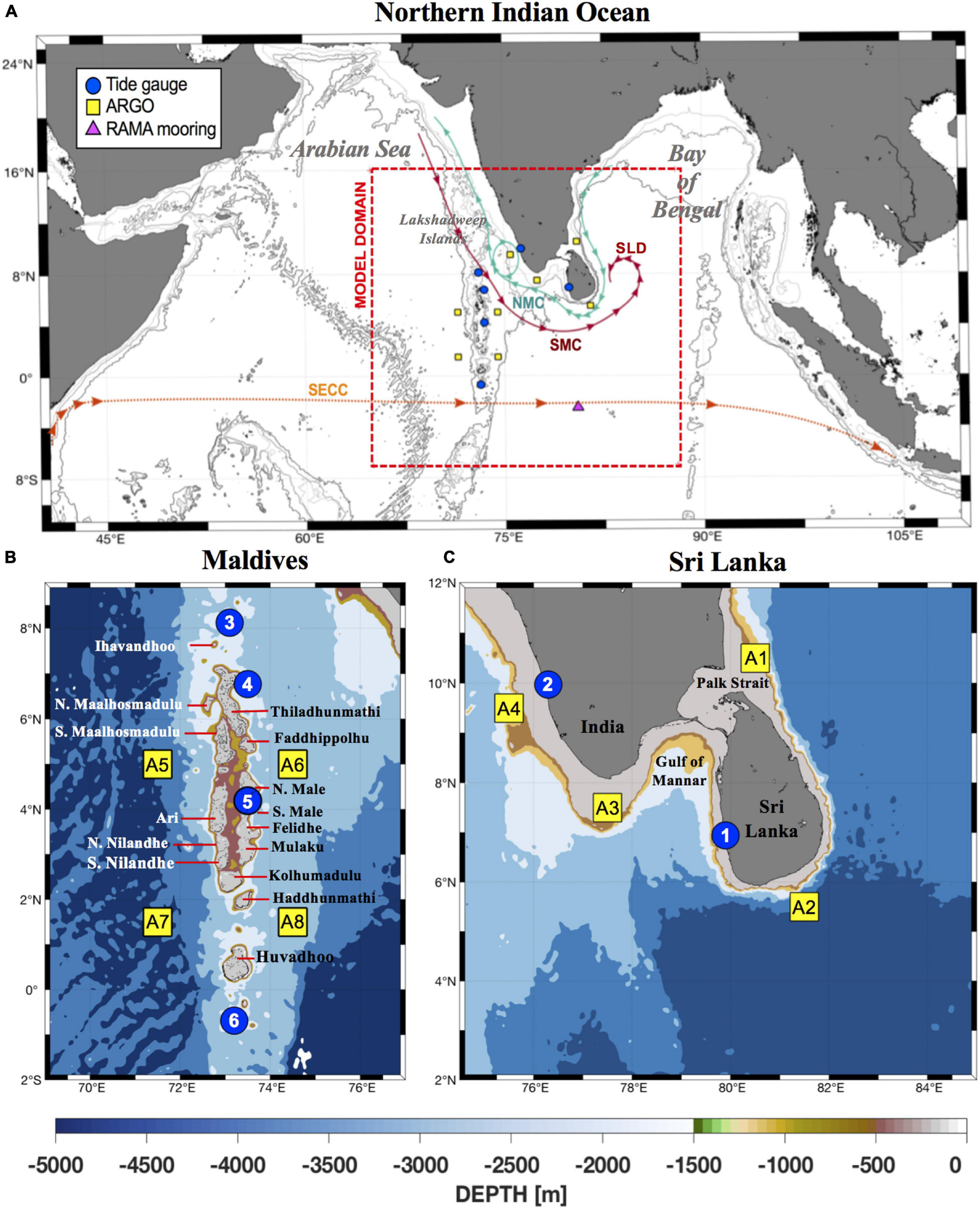
(A) Schematics for the surface circulation in the Northern Indian Ocean (NIO) adapted from Schott and McCreary, 2001. The major currents during the Northeast Monsoon (Dec–Feb) and the Southwest Monsoon (Jun–Aug) are the Northeast Monsoon Current (NMC—green line), the Southwest Monsoon Current (SMC—red line), and the Sri Lanka Dome (SLD), respectively. Also included is the South Equatorial Counter Current (SECC—orange line). The red box represents the boundaries of the model domain. The locations of ARGO profile data (yellow boxes), tide gauges (blue circles), and mooring (pink triangle) used for model validation are also identified. (B) Bathymetry map of the Maldives and atoll names. Tide gauge sites are (3) Minicoy, India (4) Male, Maldives (5) Hanimaadho, Maldives (6) Gan, Maldives based on data obtained from the University of Hawaii Sea Level Center (UHSLC—https://uhslc.soest.hawaii.edu/). Locations for ARGO profile data extraction (A5–A8) were selected based on data availability and where the IME has been previously identified from remote sensing data. (C) Bathymetry map of India and Sri Lanka. Tide gauge sites are (1) Colombo, Sri Lanka and (2) Cochin, India. Locations for ARGO profile data extraction (A1–A4) were selected to coincide with the main pathways of the monsoon currents, NMC and SMC and where the IME has been previously identified from remote sensing data.
During the NEM, the monsoon winds blow from the northeast toward the southwest direction whilst winds during the SWM come from the opposite direction. This directionality is mirrored by the two monsoon currents, the Northeast Monsoon Current (NMC) and the Southwest Monsoon Current (SMC). The NMC flows westwards from the BoB, past Sri Lanka toward the Maldives, bringing lower salinity (less dense) water from the BoB to the AS during the NEM (Figure 1A). In contrast, the Southwest Monsoon Current (SMC) flows eastwards from the AS, past the northern end of the Maldives toward Sri Lanka, transporting higher salinity (more dense) water from the AS to the BoB (Figure 1A; de Vos et al., 2014b).
Satellite ocean color imagery revealed higher surface chlorophyll concentrations (SCC) downstream of the Maldives west coast (Figures 2B, 3A,C) and a filament of higher SCC was also observed along the south-west coastline of Sri Lanka during the NEM (Figure 3B). Conversely, during the SWM, satellite observations identified higher SCC to the east of the Maldives (Figures 2A, 3D,G,H) and along the south-east coast of Sri Lanka (Figures 2C, 3F). The higher SCC were advected into a recirculation feature along the east coast of Sri Lanka known as the Sri Lanka Dome (SLD) (Figures 2C, 3E, Vinayachandran and Yamagata, 1998). These areas of higher SCC can be attributed to the Island Mass Effect (IME), which has been defined by Doty and Oguri (1956) as an enhancement of primary productivity in the surrounding waters of islands and/or topographic features.
FIGURE 2
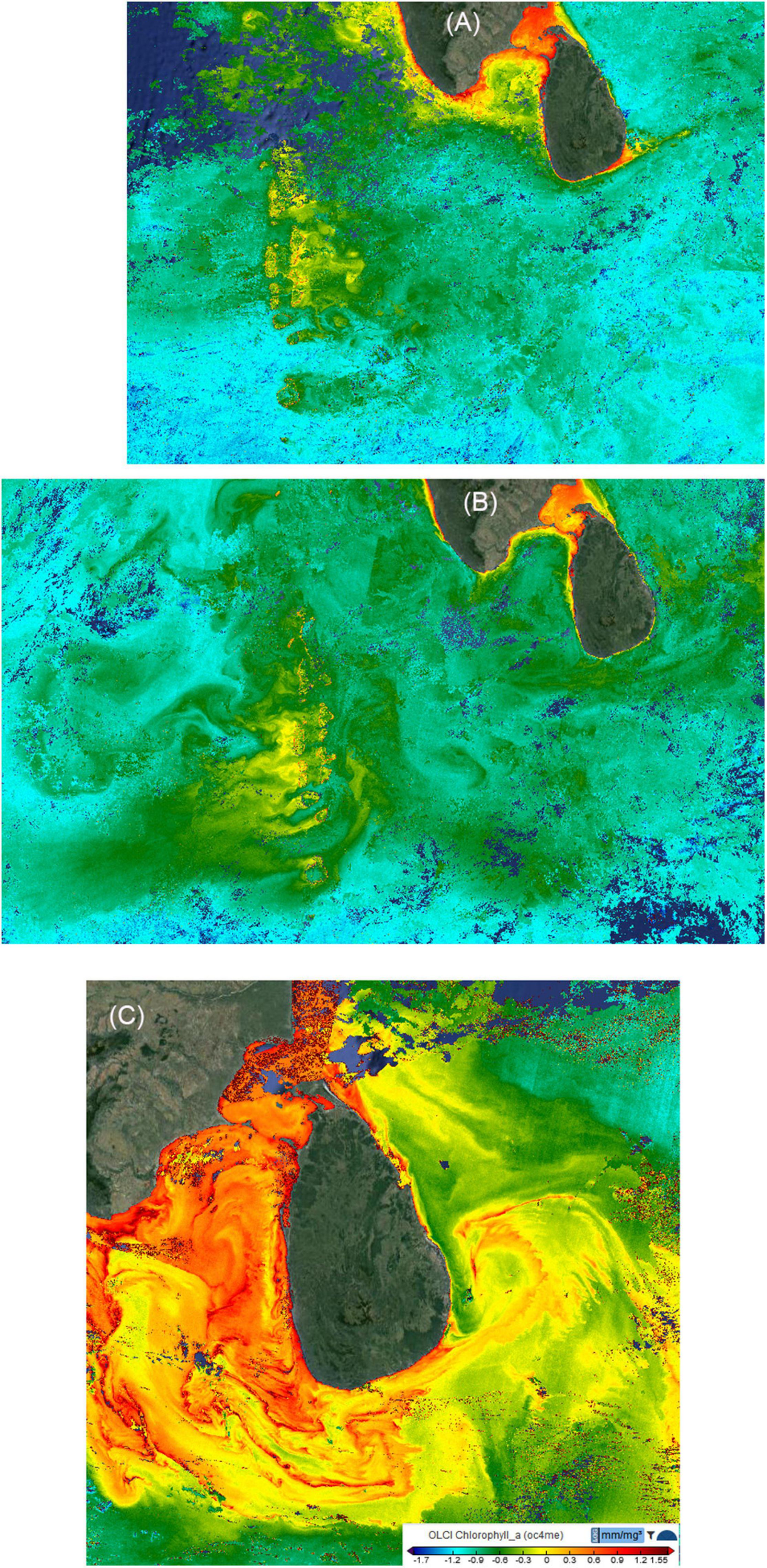
Surface chlorophyll concentrations (SCC) obtained from the Sentinel-3 satellite. (A) SWM; 7-day mean 9–15 June 2020; (B) NEM; 7-day mean 1–7 February 2020; (C) SWM; 3-day mean 10–12 August 2020. The images were sourced from https://s3view.oceandatalab.com/ and display SCC estimated using the oc4me algorithm (Morel et al., 2007).
FIGURE 3
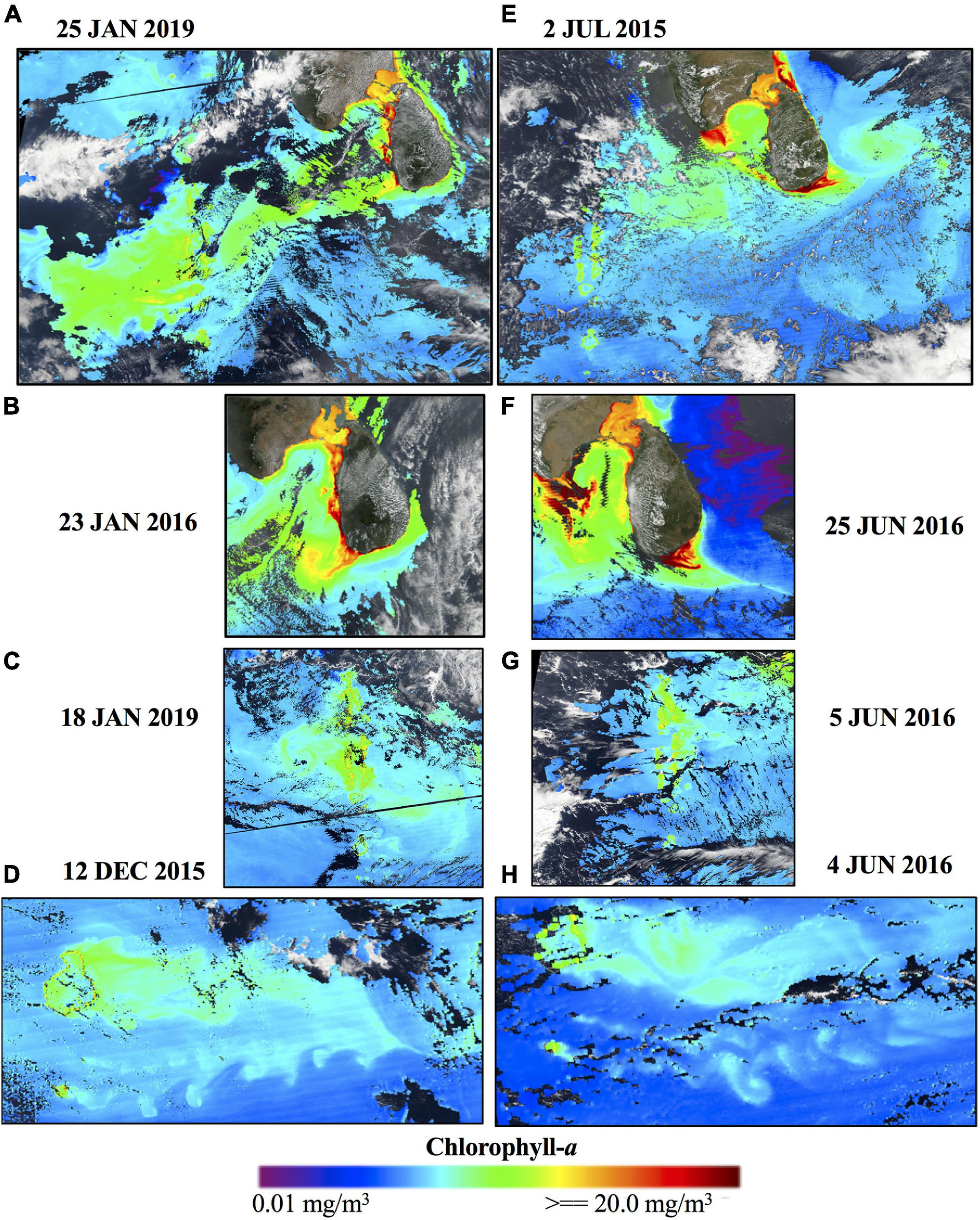
Daily snapshots of surface chlorophyll-a concentrations around Sri Lanka and the Maldives during the (A–D) Northeast Monsoon (Dec–Feb) and the (E–H) Southwest Monsoon (Jun–Aug). (A,E) Highlights potential connectivity based on the high chlorophyll-a concentrations “advected” from Sri Lanka to the Maldives. (B,F) Identifies the location of the IME along the south coast of Sri Lanka during the NEM and SWM, respectively. (C,G) Identifies the directionality of the IME along the Maldives island chain. (D,H) Displays multiple von Karman vortex streets swirling downstream from the Huvadhoo Atoll during both monsoon periods. Images adapted from EOSDIS Worldview (https://worldview.earthdata.nasa.gov).
The IME is a geographically ubiquitous phenomenon around island-atoll systems and is analogous to “an oasis in a desert” for the high primary productivity present in the island’s nearshore waters in an otherwise oligotrophic ocean (Hamner and Hauri, 1981; Caldeira et al., 2002; Elliott et al., 2012; Andrade et al., 2014; Gove et al., 2016). This increase in primary productivity can be attributed to several non-exclusive mechanisms such as tidal mixing, internal waves and lee eddies formed by flow disturbance or Ekman pumping (Gove et al., 2016). All of them involve mixing processes in the water column to bring deeper, nutrient-rich water into the photic zone, thus stimulating productivity. As such, the IME is characterized by regions of cool sea surface temperature and high current speeds due to these mixing processes (Caldeira et al., 2002). The IME is ecologically significant for its role in supporting higher trophic levels as well as influencing migratory patterns of marine megafauna and localization of fisheries around islands (Palacios, 2002; Anderson et al., 2011). The presence of the IME has been observed in various case studies worldwide such as around the Hawaiian Islands, Barbados (Cowen and Castro, 1994), Cosmoledo atolls (Heywood et al., 1990), Madeira Island (Caldeira et al., 2002), the Great Barrier Reef, Australia (Hamner and Hauri, 1981), and the Galapagos Archipelago (Palacios, 2002).
The seasonality of the NIO circulation is defined by the NEM and SWM. The key difference between the monsoons lie in the dynamics of the monsoon wind forcing, with stronger winds during the SWM (Schott and McCreary, 2001). This directly affects the strength of the monsoon currents, NMC and SMC. The NMC peaks during January with current strength approaching 0.2 ms–1 south of Sri Lanka whilst the SMC peaks during July with current strength approaching 0.4 ms–1 (Shankar et al., 2002). Due to this difference in directionality and intensity of wind forcing and currents, the type of circulation features and nature of the IME developed are unique to each monsoon period. The effects of freshwater input rainfall/runoff in the study region are limited to a narrow coastal band along the coast (de Vos et al., 2014a).
To date, there have been several studies by Anderson et al. (2011); de Vos et al. (2014b), and Sasamal (2007) that have identified the IME in the NIO via remote sensing data and numerical modeling. However, the paucity of in situ measurements in this region as well as the effect of cloud cover during the SWM meant that there have been limitations in resolving the mechanisms underlying IME development. In addition, coarser global/regional models currently are unable to resolve the fine-scale features implicit to the IME.
The Maldives island chain (Figure 1B) is one of the largest and most geologically complex mid-ocean atoll chains in the world. It extends ∼1,000 km from Ihavandhoo (∼8°N) to Gan (∼1°S), and consists of ∼ 1,200 small coral islands and sandbanks (Figure 1B). The islands have a mean elevation of 1–1.5 m above sea level. The coral islands are grouped in a double chain of 27 atolls that run north to south (Figure 1B). These atolls are situated atop a submarine ridge that rises abruptly from the depths of the Indian Ocean and runs from north to south. The depth of the surrounding ocean are >4,000 m (Figure 1B). Along the ridge, there are many coral islands with intervening channels with depths <50 m where water can flow zonally and allows for the generation of shallow island wakes (Figures 2A,B). At the southern end of the Maldives, there are two deep passages between Kolhumadulu, Haddhunmathi, and Huvadhoo (Figure 1B). In contrast, although Sri Lanka is an island, from an oceanographic point of view, it behaves as a large headland due to the very shallow waters (<20 m) off the northern section of the island (Figure 1C). The continental shelf around Sri Lanka is narrower, shallower and steeper than the global mean (de Vos et al., 2014b) with the width of the shelf along the southern coast less than 10 km (Figure 1C). The continental slope around Sri Lanka is a concave feature that extends from 100 m to 4,000 m in depth. Thus, the Maldives and Sri Lanka have similar yet contrasting bathymetric features, i.e., they both have narrow continental shelves/slopes with the surrounding ocean depths generally >4,000 m.
In this paper, we examine the influence of the reversing monsoon currents on the variability of the IME around Sri Lanka and the Maldives archipelago and the IME structure through the water column. Specifically, we focus on the IME developed due to island wakes that have been generated through the interaction between oceanic currents and topography, i.e., the bathymetrically distinct Maldives and Sri Lanka. This was undertaken through the development and application of a high spatial resolution three-dimensional numerical model for the region to characterize the structure of the IME across seasonal time scales.
The paper is organized as follows: section “Materials and Methods” describes the model configuration in detail and evaluates the robustness of the model against observational data; section “Results” examines the variability of the IME at both seasonal and intra-seasonal scales and section “Discussion” is the discussion followed by the concluding remarks and summary in section “Summary and Conclusion.”
Materials and Methods
Numerical Model Configuration
The numerical model was built using the Rutgers University version of the Regional Ocean Modeling System (ROMS)1 with significant adaptations for Maldives and Sri Lanka. It has been previously used to study island wake circulation in the southern California Bight (Caldeira et al., 2005; Dong and McWilliams, 2007), the Hawaiian Islands (Kersalé et al., 2011), the Marquesas Archipelago (Raapoto et al., 2018), New Caledonia (Marchesiello et al., 2010), and Fernando de Noronha Island (Brazil) (Tchamabi et al., 2017). It was also used to examine the circulation patterns around Sri Lanka and the SLD (de Vos et al., 2014b). ROMS is a split-explicit free surface, terrain-following vertical coordinate oceanic model, and resolves the incompressible primitive equations (Cushman-Roisin and Beckers, 2011) using the Boussinesq approximation and hydrostatic vertical momentum balance (Shchepetkin and McWilliams, 2003, 2005). These equations are discretized on an orthogonal, curvilinear, Arakawa C-grid and a stretched, terrain-following coordinate system in the vertical direction (Song and Haidvogel, 1994; Shchepetkin and McWilliams, 2003, 2005).
The model grid domain extends from 7°S–15°N, 65°E–88°E (Figure 1A). Bathymetry was obtained from the General Bathymetric Chart of the Oceans (GEBCO) 30 arc-second gridded product (Weatherall et al., 2015)2 and coastline data was extracted from GSHGG coastlines3. Potential horizontal gradient errors were minimized by smoothing the bathymetry until the recommended slope factors were obtained for the Beckman and Haidvogel number, rx0 <0.2 (topographic stiffness ratio) (Beckmann and Haidvogel, 1993) and the Haney number, rx1 (hydrostatic instability number), was 7 > rx1 > 5 (Haney, 1991). The bathymetry was smoothed in the following steps: (1) a Shapiro filter was applied twice across the original bathymetry; (2) High rx0 areas >0.2 were identified (Supplementary Figure 1A). Iterative pointwise smoothing was applied at these high rx0 areas (Supplementary Figure 1A). This was found to achieve a good balance in maintaining realism without compromising grid stability. rx1 was sensitive to the vertical parametrization in the model which was dependent on the number of vertical layers (N), the thermocline depth (Tcline) and the s-coordinate surface (θS) and bottom control parameters (θb). The representation of surface mixed layer processes was sensitive to the vertical resolution at the surface, which is dependent on the choice of stretching functions, i.e., the vertical terrain-following stretching function (VStretch) and vertical terrain-following transformation function (VTransform). A summary of the values used for these parameters are provided in Supplementary Table 1 and the model’s vertical grid resolution in Supplementary Figure 2.
The model domain had a depth range of 0–5,000 m with 30 vertical layers (Supplementary Figure 2). The thermocline depth was estimated from the ARGO climatology profile averaged across the entire model domain. The resulting horizontal grid resolution was approximately 3 km per cell in the 860 × 860 grid. The higher spatial resolution was necessary since the horizontal scales of these island wake structures have a small Rossby radius of deformation. The initial conditions and open boundary data (salinity, temperature, sea surface height and velocity fields) for the model were obtained from the 1/12° global US Navy Hybrid Coordinate Ocean Model (HYCOM) GLBu0.08 (Expt 19.1–91.2) reanalysis product (Chassignet et al., 2007). It should be noted that this product is without tides.
Due to the difference in bathymetry between the z-coordinate HYCOM reanalysis product and model s-coordinate grid, a hybrid bathymetry was created using both the GEBCO and HYCOM bathymetry to improve interpolation at the boundaries (Supplementary Figure 3). The reanalysis product and hybrid bathymetry were then gridded to the model grid boundaries for the final boundary files. Tidal constituents were obtained from the TPXO7 global tide model with a 1/4° resolution (Egbert and Erofeeva, 2002) to generate the tidal forcing and was applied to the four open boundaries using the Flather condition (Flather, 1976) and Chapman implicit boundary condition for the elevation. For the baroclinic mode (temperature, salinity, and baroclinic momentum), a combination of Orlanski-type radiation boundary conditions were applied with nudging (Marchesiello et al., 2001). Vertical mixing processes were parameterized with the non-local K-profile boundary layer scheme (Large et al., 1994) and implemented for both surface and bottom boundary layers. In addition, a sponge layer was applied across 60 grid points (approximately 180 km) where the viscosity was increased linearly from the interior to a maximum viscosity of 300 m2 s–1 at the exterior. Explicit lateral viscosity was set to zero throughout the model domain, except along the sponge layer near the open boundaries. The model was nudged toward daily HYCOM data along a linearly tapered nudging band along the open boundaries that had the same dimensions as the sponge layer (60 grid points). The model set up and parameters have been similarly applied by Wijeratne et al. (2018) for Australian waters.
At the surface, the model was forced with 3-hourly atmospheric pressure and wind stress at 10 m, net heat and freshwater fluxes at a 1/8° resolution obtained from the European Centre for Medium Range Weather Forecast (ECMWF) ERA-Interim reanalysis dataset (Dee et al., 2011). To prevent the simulation from drifting, the surface data were relaxed to daily surface fields from HYCOM [sea surface temperature (SST), sea surface salinity (SSS)] and a heat flux correction (maximum 37°C) that was derived from the HYCOM SST averaged over the region was applied.
The ROMS simulation, hereafter referred to as SNIO, was run over a 12 year period between the years 2005–2016 with daily outputs saved. The model took about 6 months to reach statistical equilibrium and was dependent on the initial conditions used, in this case the hydrography from HYCOM. To avoid impact from the model spin-up on the results, only model outputs from year 2006 onward were used.
Model Validation
The model results were validated against several observational datasets for the following variables: sea level, temperature, salinity, and surface current velocities. A summary of the observational data, time period and source that were used for model comparison are presented in Table 1.
TABLE 1
| Variable | Source | Period | Location | Model location | RMSE | Bias | MAE | R2 | Skill |
| Sea surface height | UHSLC https://uhslc.soest.hawaii.edu/ | Sri Lanka 2006–2016 | (1) Colombo | 79.9°E, 6.94°N | 0.45 | –0.05 | 0.44 | 0.78 | 0.62 |
| India 2011–2016 | (2) Cochin | 76.2°E, 9.96°N | 0.43 | –0.06 | 0.41 | 0.82 | 0.60 | ||
| (3) Minicoy | 73.1°E, 8.11°N | 0.41 | –0.04 | 0.41 | 0.83 | 0.54 | |||
| Maldives 2006–2016 | (4) Male | 73.5°E, 4.20°N | 0.43 | –0.04 | 0.42 | 0.47 | 0.12 | ||
| (5) Hanimaadhoo | 73.2°E, 6.76°N | 0.42 | –0.04 | 0.42 | 0.73 | 0.32 | |||
| (6) Gan | 73.1°E, 0.78°S | 0.44 | –0.43 | 0.43 | 0.20 | 0.24 | |||
|
|
|||||||||
| Period | Velocity | RMSE | Bias | MAE | R2 | Skill | |||
|
|
|||||||||
| Current velocities | OSCAR https://www.pmel.noaa.gov/tao/drupal/disdel/ | 2006–2016 | NEM | U | 0.19 | 0.03 | 0.13 | 0.60 | 0.70 |
| V | 0.09 | –0.02 | 0.07 | 0.44 | 0.41 | ||||
| SWM | U | 0.25 | –0.01 | 0.18 | 0.88 | 0.67 | |||
| V | 0.13 | 0.02 | 0.08 | 0.39 | 0.34 | ||||
| Sea surface temperature | MODIS https://modis.gsfc.nasa.gov/data/dataprod/ | 2006–2016 | NEM | 0.40 | 0.18 | 0.25 | 0.82 | 0.79 | |
| SWM | 0.43 | 0.24 | 0.32 | 0.65 | 0.70 | ||||
| Temperature, salinity | ARGO http://www.godac.jamstec.go.jp/argogpv/e/ | 2006–2016 | 1.33 | –2.5 | 1.89 | 0.53 | 0.66 | ||
Observational data sets used for model validation and statistical metrics.
The following statistical metrics were used for validation—Pearson correlation coefficient (Coefficient of determination, R2), the Root-Mean Square Error (RMSE), the model bias, the mean absolute error (MAE), and Willmott model skill (Willmott, 1982). The statistical metrics for each variable are consolidated in Table 1.
Sea Level
Tide gauge data and locations around the Maldives (Figure 1B) and Sri Lanka (Figure 1C) were obtained from the University of Hawaii Sea Level Centre (UHSLC). The sea level computed from the model were compared to the tide gauge data (Figure 4) and the monthly climatologies were averaged between 2006 and 2016 for the Sri Lanka and Maldives stations and 2011–2016 for India (Table 1). The higher sea levels associated with the SWM period (June- August) are reproduced in the model. The model generally underestimated the sea level at the specified locations but performed better (Figure 4 and Table 1) around Sri Lanka and India compared to the Maldives (Figure 4 and Table 1). Possible reasons for this error could be due to the complex bathymetry around the Maldives that may have been overly smoothed to avoid potential horizontal pressure gradient errors and that the minimum depth of the model was set to 10 m which was deeper than the actual depth of the tide gauge locations. In addition, some of the locations extracted from the model could not be exactly matched to the locations of the tide gauges since those fell within the land mask area of the model (Table 1).
FIGURE 4
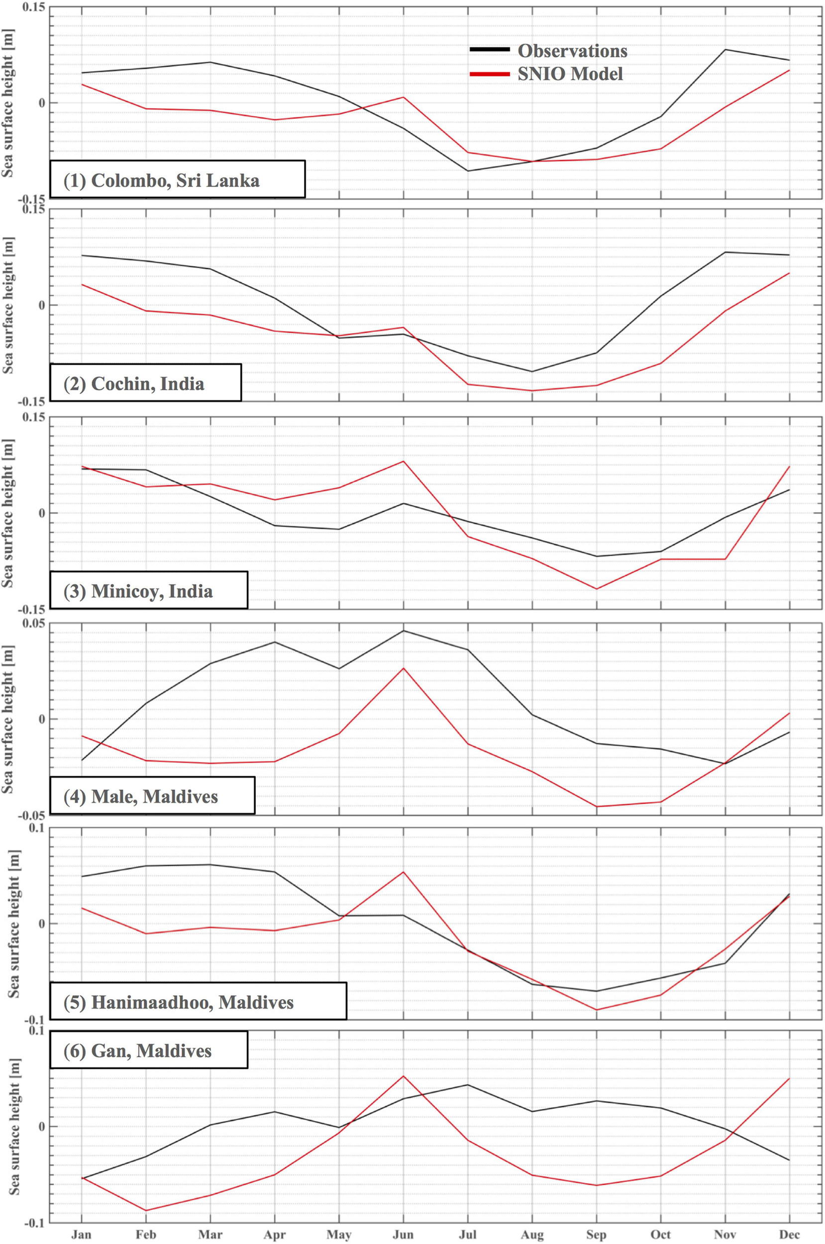
Monthly climatology of observed sea level derived from UHSLC observations (black line) and SNIO model (red) from tide gauge locations at (1) Sri Lanka, Colombo (2) Cochin, India (3) Minicoy, India (4) Male, Maldives (5) Hanimaadhoo, Maldives (6) Gan, Maldives. All units are in (m).
Sea Surface Temperature
Throughout the 11 years of model simulations, the model was able to reproduce the regional seasonal SST pattern but with the largest difference during the SWM. The mean difference between the model and satellite derived observations was <1°C for both monsoons (Figures 5C,I). Comparisons between the climatology of the MODIS SST and the model SST indicated that although the bias was low for both monsoon periods (Table 1), the general distribution of SST differences were not consistent (Figures 5C,I). The model tended to slightly overestimate SST in the region of the South Equatorial Counter Current (SECC) (2°S–2°N) and underestimates SST around the islands (Figure 5 and Table 1) particularly the shelf area between India and Sri Lanka by a mean difference of <2°C (Figure 5). This discrepancy could be due to the bottom reflectance from the shallow depth in this shelf region (<10 m) which has been known to affect the estimation of MODIS measurements (Jiang et al., 2017). Conversely, the overestimation of temperatures occurred closer to the SECC region (Figure 5). During the NEM, the model has a lower bias (0.18) compared to the SWM (0.24) and the largest difference in SST was localized around the Lakshadweep Islands. However, during the SWM, the largest SST difference was more pronounced between the shelf region of Sri Lanka and the south point of India. Overall, the model exhibits a strong skill (Skill > 0.6, RMSE < 0.5, Table 1) to simulate the surface SST.
FIGURE 5
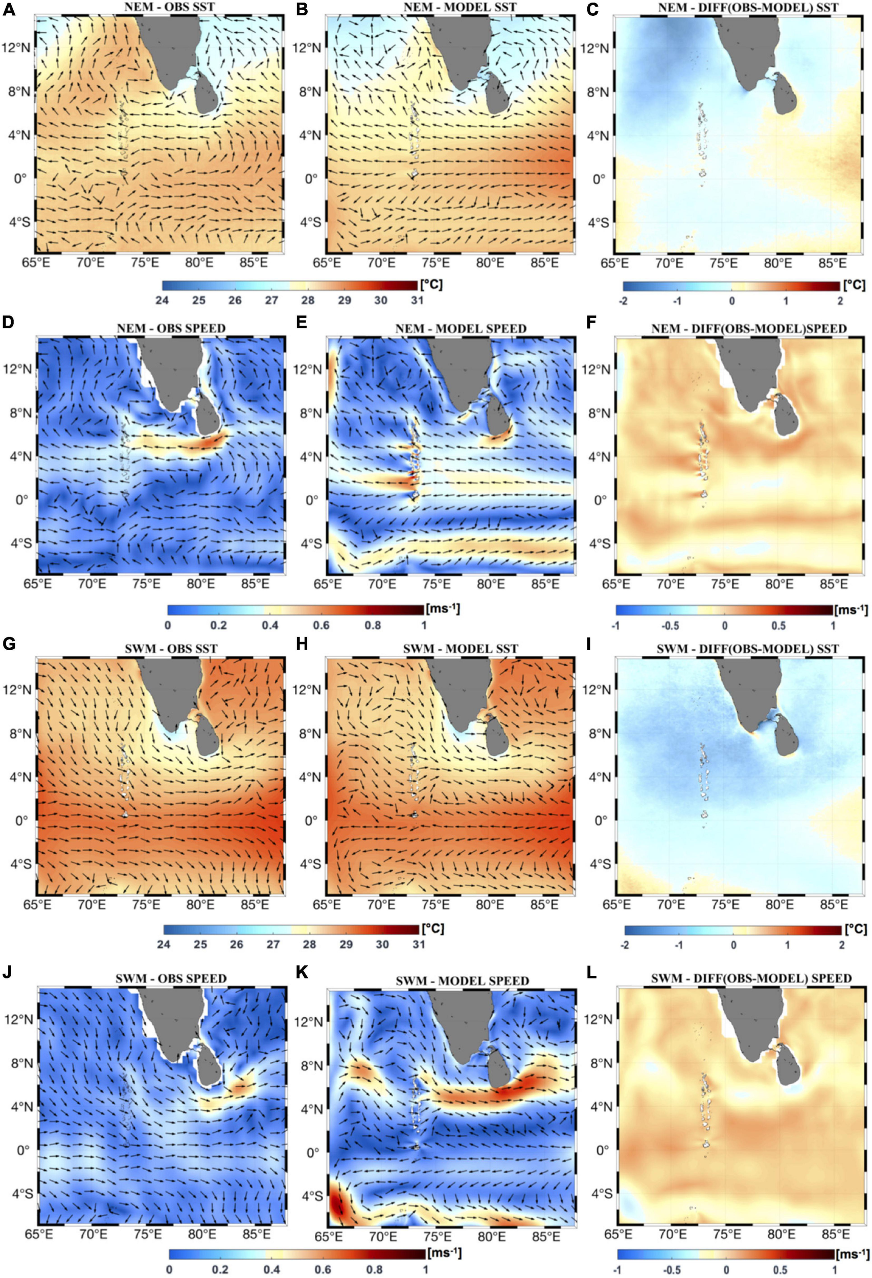
Seasonal climatology of SST and current speeds of observations and model simulations during the NEM (A–F) and SWM (G–L) averaged over 2006–2016. Observational SST was obtained from MODIS-AQUA and mapped with current velocities from OSCAR (arrows) (A,G). SNIO model SST from were mapped with model current velocities (B,H). The difference between the observations and model SST were also calculated (C,I). Observational current speeds were calculated from OSCAR and mapped with current velocities (arrows) (D,J). SNIO model current speeds from were mapped with model current velocities (E,K). The difference between the observations and model current speeds were also mapped (F,L).
Current Velocities
The model has higher current speeds than the observational data (Figures 5F,L). The model performed slightly better for the zonal velocities (Skill > 0.65, Table 1) compared to the meridional velocities (Skill < 0.5, Table 1) where the mean difference for the zonal velocities and meridional velocities were 0.03 ms–1 and 0.06 ms–1 for the NEM and SWM, respectively. This overestimation could be attributed to the higher resolution of the model compared (3 km) to the satellite observations (4 km).
Vertical Temperature Profiles
Model validation with the ARGO vertical profiles were conducted at eight locations around the Maldives and Sri Lanka (Figure 1). The mean monthly climatology of ARGO temperature during 2006–2014 was compared with the mean monthly climatology from the model at those areas and plotted with depth (Figure 6). Overall, the model had good agreement (RMSE = 1.3°C, Skill > 0.6, Table 1) with the Argo data and the simulated profiles were able to represent the changes in the thermocline depth for the different regions in the model domain. However, the model tended to underestimate temperatures compared to the observational data and this difference is apparent at depths less than 600 m (Table 1).
FIGURE 6
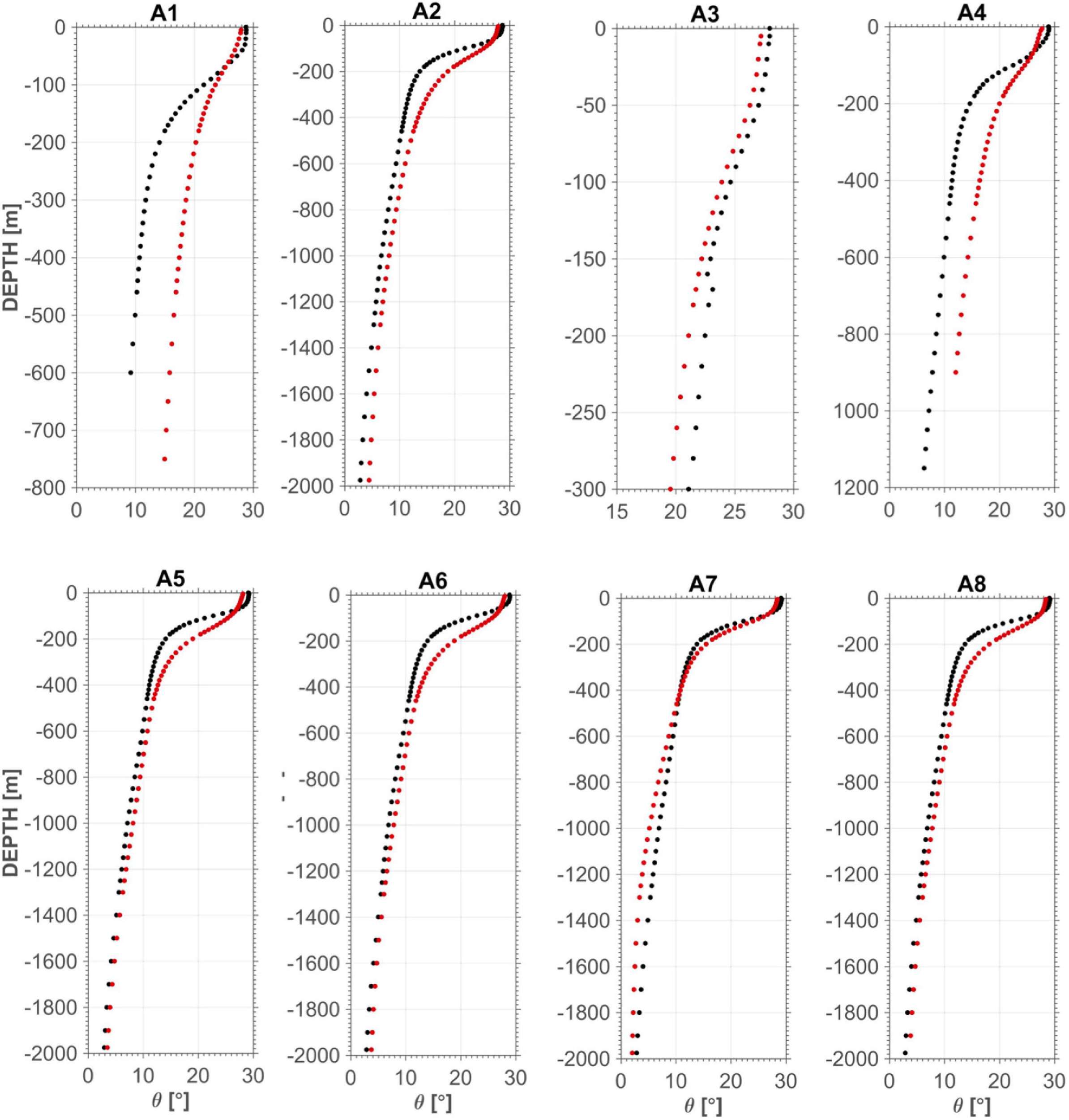
Comparison of Argo (black) and SNIO (red) climatological monthly mean temperature profiles at eight locations identified around Maldives and Sri Lanka (see Figure 2). Note that the y-axis are at different scales.
Volume Transport
Volume transport at the RAMA mooring (Figure 1A) was calculated from the model at 80.5°E, 2.5°S–2.5°N and depth integrated over 80 m for both the NEM and SWM during 2005–2016. The negative direction of the volume transport indicates that the main directionality of the currents heading westwards and the transport values were in good agreement (Figure 7) with McPhaden et al. (2015). The mean transport values were in the range of 9–11 SV (Figure 7) while McPhaden et al. (2015) had transports of 5–15 Sv. The westward mean flow was attributed to the mean residual of the monsoon currents above the equator (McPhaden et al., 2015). The SWM had higher volume transport with a mean value of 10 Sv compared with the NEM mean value of 7 Sv (Figure 7).
FIGURE 7
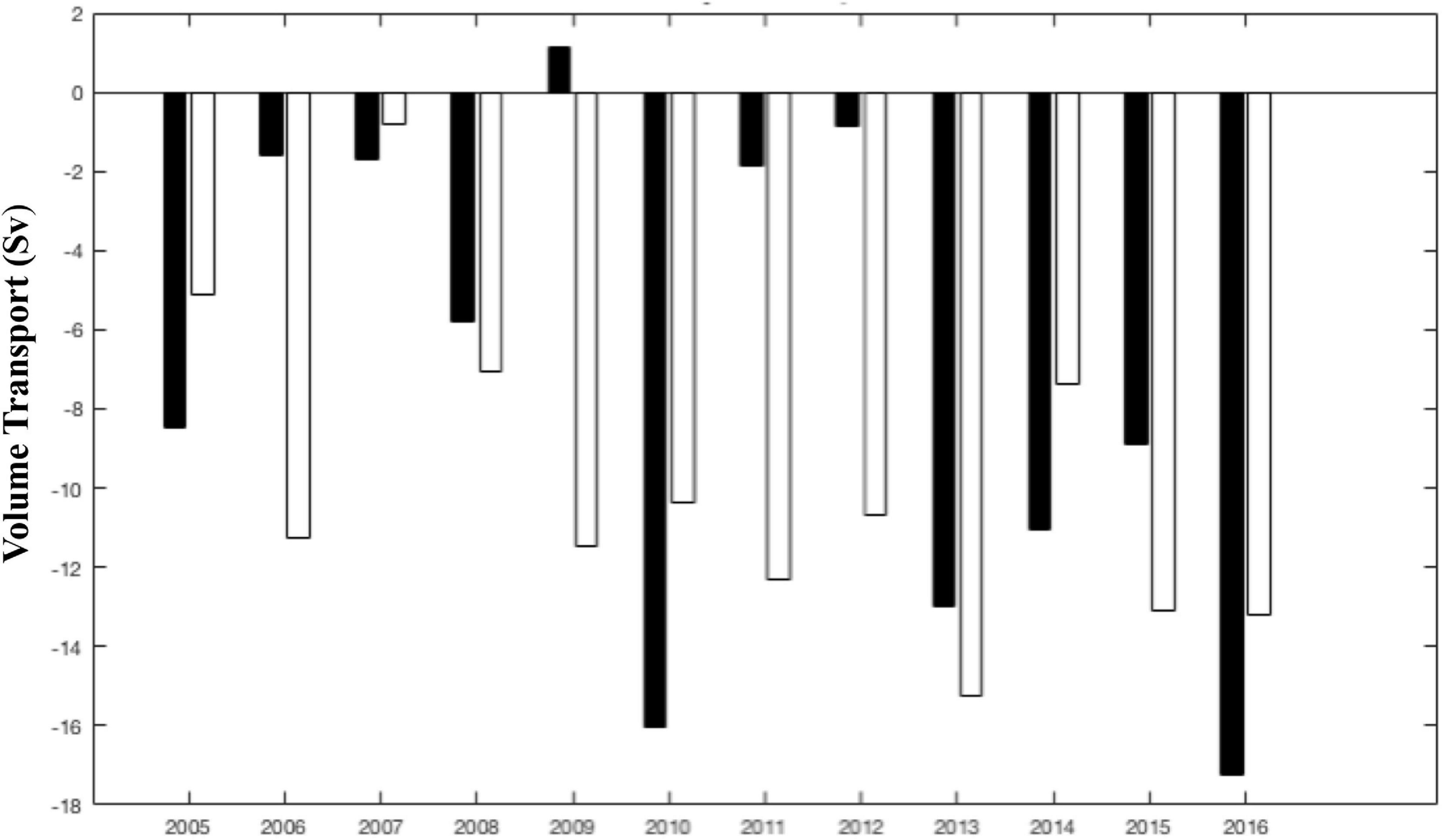
Volume transport from model output at 80.5°E across 2.5°S–2.5°N, relative to a fixed depth of 80 m for the NEM (black) and SWM (white) during 2006–2016.
Results
Seasonal Circulation Variability
Surface Circulation
The mean surface current speed for the entire domain during the simulation SWM was 0.3 ms–1 whilst the mean speed during the NEM was 0.2 ms–1 (Figure 5). During the NEM, current speeds >0.3 ms–1, along the east coast of India indicated the presence of the East Indian Coastal Current (EICC) as it flows southwards along the coastlines of eastern India and Sri Lanka. However, along the southern coast of Sri Lanka, current speeds increased to >0.5 ms–1 before part of the current continued to form the West Indian Coastal Current (WICC) along the west coast of India (Figure 5). Several island wakes developed along the western coastline of the Maldives with the largest, in terms of spatial extent and current speed (>0.5 ms–1), located at 5 and 1°N (Figure 5). All the wakes were directed westward and the largest wake at ∼1°N extended up to 780 km. The SECC was also present between ∼4 and 6°S throughout the study region and had a mean current speed of ∼0.4 ms–1.
During the SWM, the SMC (speed > 0.5 ms–1) enters the model domain from 4 to 8°N to flow eastwards past the northern tip of the Maldives archipelago and past the southern coast of Sri Lanka (Figure 8). The major flow pathway was such that the currents flowed southwards, parallel to the Maldives in the west and then flowing northwards along the eastern side of the Maldives. This was due to the presence of the submarine ridge. Weaker eastward flow across the atolls were present which developed into island wakes that were visible in satellite imagery (Figure 2). There was a distinct separation of the current pathways between Maldives and Sri Lanka. The flow from the west was deflected to the south by the Maldives ridge. The currents that impacted Sri Lanka during the SWM was mainly derived from the WICC with the injection of colder water through upwelling along the southern tip of India (Figure 8). The advection of this cold water along the southern coast of the Sri Lanka that acts as a headland resulted in the formation of the recirculation feature identified as the SLD.
FIGURE 8
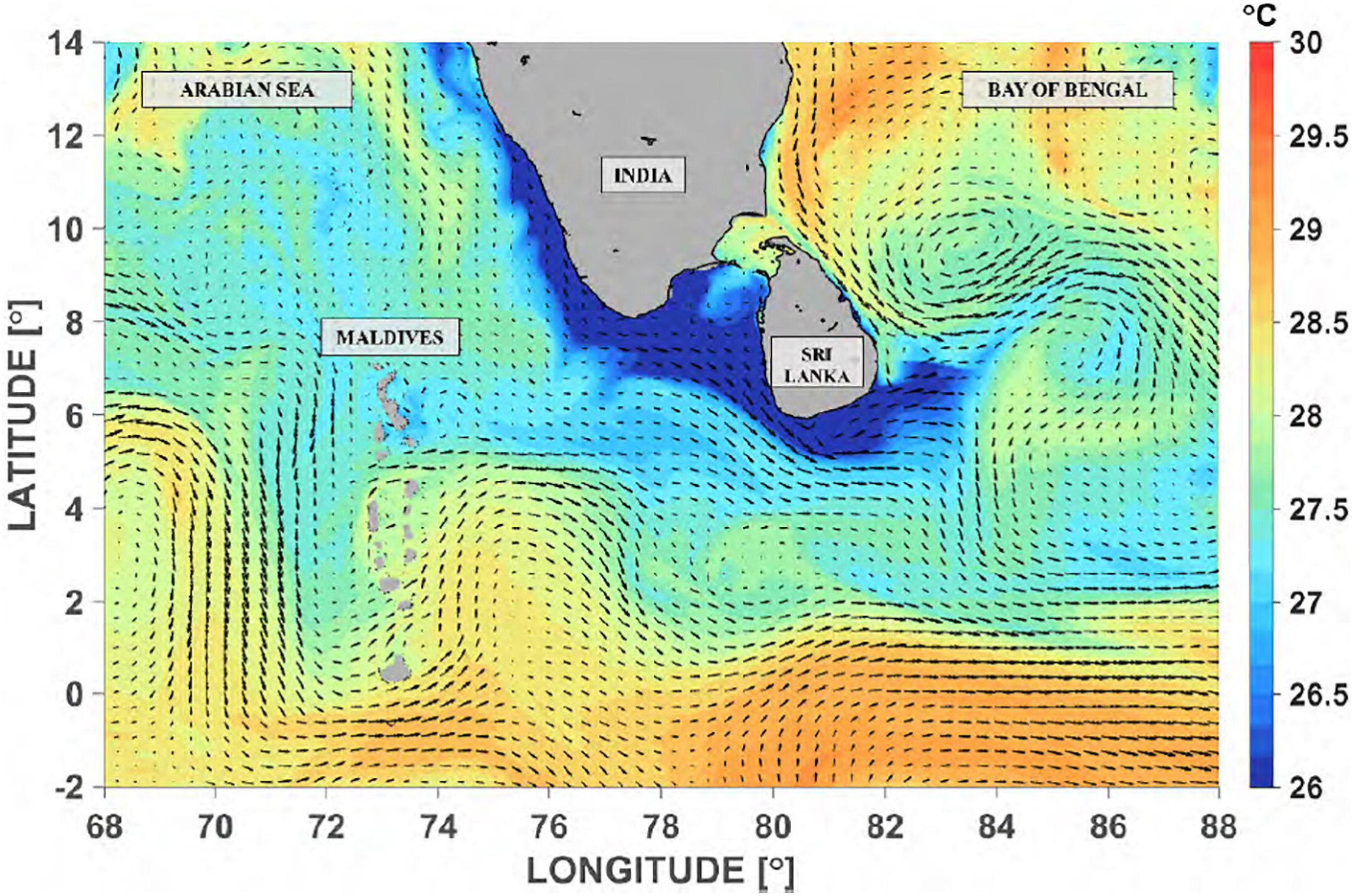
Surface flow patterns (arrows) and sea surface temperature (color) in July, during the SWM showing the circulation around the Maldives and flow separation and the formation of the Sri Lanka Dome to the east of Sri Lanka.
Thermocline Variability
To identify locations of upwelling and downwelling, the depth of the 26°C isotherm (henceforth, referred to as D26) was extracted and mapped from the model climatology (Figure 9). D26 is often used in the NIO (McCreary et al., 1993; Rao et al., 2006; Ali et al., 2015; McPhaden et al., 2015) whilst D20 (depth of the 20°C isotherm) is used more in the Southern Indian Ocean. Here, we define upwelling (downwelling) processes to be when the local D26 is shallower (deeper) than the domain-averaged mean depth for D26. There are several distinct differences between the NEM and SWM, the first being that downwelling was more prevalent during the NEM and upwelling during the SWM. The mean depth for D26 during the NEM was ∼112 m whilst during the SWM, the mean depth for D26 was ∼100 m.
FIGURE 9
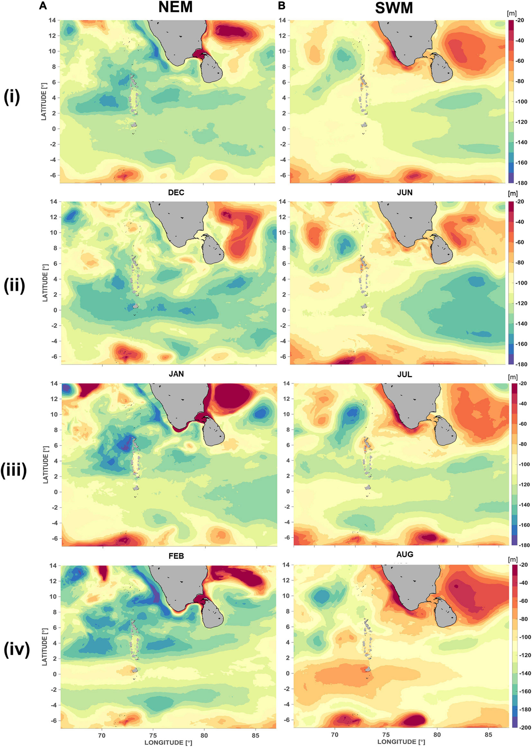
Mapped depths of the 26°C isotherm (D26) relative to the mean during the (A) NEM (i) December (ii) January (iii) February and (B) SWM—(i) June (ii) July (iii) August. Shallower (deeper) values where the colormap is warmer (cooler) identify locations where the 26°C isotherm (D26) is uplifted (suppressed).
During the NEM, downwelling occurred on both sides of the Maldives island chain but upwelling occurred within the archipelago and downstream from Kolhumadulu Atoll (73.5°E, 0.5°N). Upwelling occurred along the south coast of Sri Lanka and India (Figure 9Ai). D26 reached its shallowest at approximately 83°E, 13°N (D26 < 50 m), indicating the presence of strong upwelling. At the start of the NEM during December, the mean depth of D26 was ∼113 m and downwelling occurred on the western coastline of the Maldives Island chain (Figure 9Aii). It was deepest along 3 and 0.5°N. Around the eastern coastline of Sri Lanka, D26 shallowed to depths <50 m from the surface between ∼7 and 13°N. Downwelling intensified during January with D26 being suppressed to depths >160 m and the overall mean depth increasing to ∼115 m (Figure 9Aiii). The downwelling signal was strongest along the northern tip of the Maldives at ∼7°N and extended further westward across ∼4°N. In contrast, upwelling strengthened along the east coast of India and downwelling occurred at ∼86°E, 12°N. Upwelling reached its maximum along the southern coast of Sri Lanka during January with D26 being shoaled to less than 80 m from the surface. In February, downwelling intensity subsided (mean depth of D26 at ∼110 m) but was more prevalent across the domain with downwelling occurring both around Maldives and the south coast of Sri Lanka Sri Lanka. However, upwelling also developed along the western coastline of Maldives at ∼5°N and downstream from Kolhumadulu Atoll (Figure 9Aiv).
Downwelling during the SWM tends to occur to the south of 5°N for the Maldives but occurs at the northern tip of the Maldives (Figure 9Bi). Upwelling intensifies along the south coast of Sri Lanka where the mean depth of D26 has been shoaled by approximately 20 m to the surface. In addition, strong upwelling between 82 and 86°E identify the presence of the Sri Lanka Dome (Figure 9Bi). The SWM was characterized by increased wind stress with monsoonal currents flowing eastward and overall upwelling favorable. However, upwelling is continuous throughout the domain and there are key differences around the Maldives and Sri Lanka. The mean depth of D26 across the domain was 105 m in June (Figure 9Bii) and shallowed to 100 m in July (Figure 9Biii) and shallowest in August at 95 m (Figure 9Biv). Upwelling was at a maximum both spatially and in intensity at the northern tip of the Maldives at ∼6°N in June but subsided in July (Figure 9Biii). In August, downwelling developed at this location. Below 5°N, downwelling was prevalent along the eastern coastline from June to July but the reverse occurred during August. At ∼1°N, D26 was gradually uplifted from ∼140 m in June to a maximum of ∼50 m in August. Along the south coast of Sri Lanka, upwelling is initiated in June and reached its maximum in August (Figure 9Biv). In the region where the SLD has been known to develop, upwelling started at ∼82°E, 8°N and broadened during July, reaching its maximum at ∼30 m depth from the surface (Figure 9Biii).
Intra-seasonal Circulation Variability
Meridional transects of temperature were examined along the eastern coastline of the Maldives at 73 and 74°E, and the south coast of Sri Lanka at 81°E for the monthly mean average from the model output and compared within each monsoon period (Figures 10, 11). The remote sensing data and numerical simulations indicated the formation of island wakes frequently occurs on the downstream of the islands (Figures 2, 5). This was the motivation for the selection of these, hence these sections. For consistency, we define cooler temperatures <27.5°C and warmer temperatures >27.5°C.
FIGURE 10
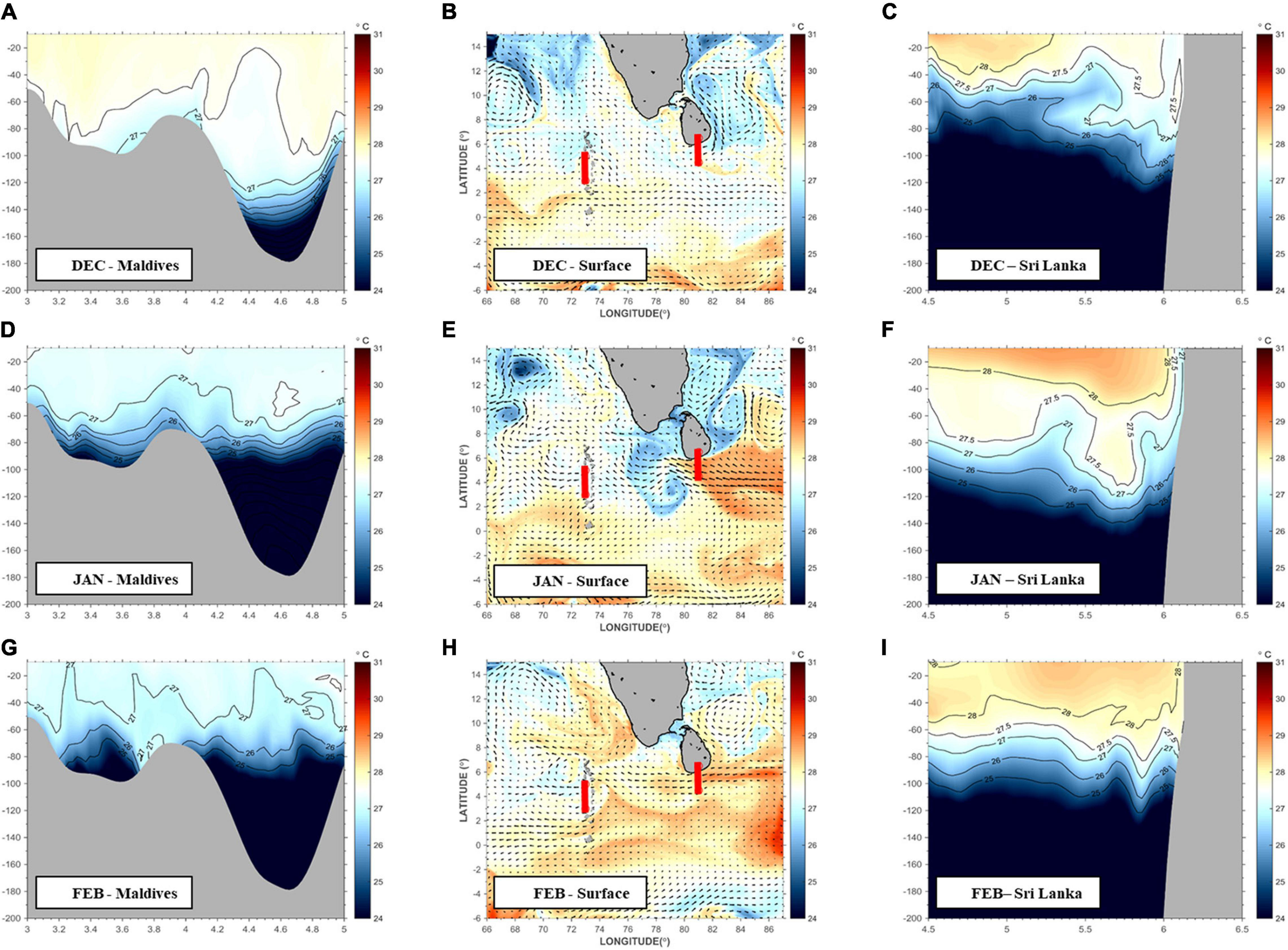
Top to bottom: NEM model output for December, January, and February. Left panel shows the longitudinal temperature transect for Maldives along 73°E and the right panel shows the longitudinal temperature transect for Sri Lanka along 81°E. Surface circulation and temperature for the model domain is shown in the middle panel and red lines indicate transect locations. Intra-seasonal temperature variability during the NEM for Maldives and Sri Lanka during (A–C) December, (D–F) January, (G–I) February. Longitudinal temperature transects for Maldives along 73°E are shown in (A) December (D) January (G) February. Surface circulation and temperature for the model domain is shown (B) December (E) January (H) February. Longitudinal temperature transects for Sri Lanka along 81°E are shown in (C) December (F) January (I) February.
FIGURE 11
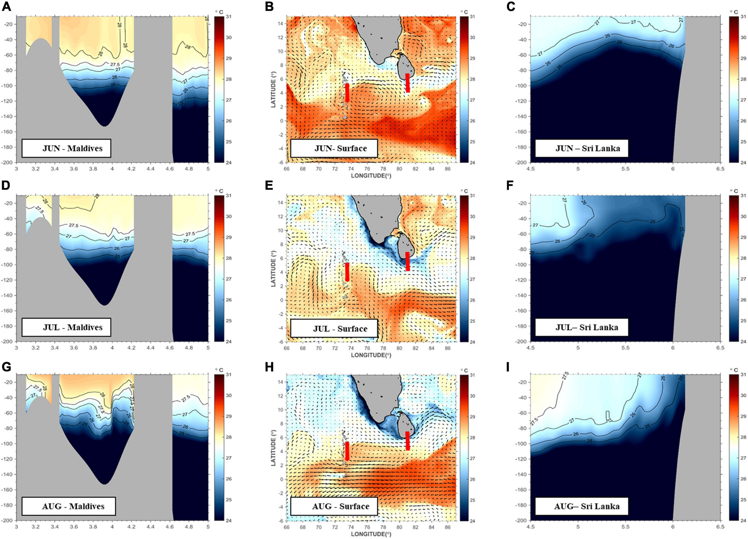
Top to bottom: SWM model output for June, July, and August. Left panel shows the longitudinal temperature transect for Maldives along 74°E and the right panel shows the longitudinal temperature transect for Sri Lanka along 81°E. Surface circulation and temperature for the model domain is shown in the middle panel and red lines indicate transect locations. Intra-seasonal temperature variability during the SWM for Maldives and Sri Lanka during (A–C) June, (D–F) July, (G–I) August. Longitudinal temperature transects for Maldives along 73°E are shown in (A) June (D) July (G) August. Surface circulation and temperature for the model domain is shown in (B) June (E) July (H) August. Longitudinal temperature transects for Sri Lanka along 81°E are shown in the right panel for (C) June (F) July (I) August.
Northeast Monsoon (December to February)
At the start of the NEM during December, currents begin the transition from the inter-monsoon period and begin to flow east to west. The EICC strengthens along the east coast of India before making its way to Sri Lanka and the interaction along the curvature of the Sri Lanka coastline is accompanied by cooler SST and strong currents (Figure 10B). The EICC follows the coastline tightly and part of it becomes entrained within a recirculation feature along the south coast before the remaining current flows northwards into the Bay of Bengal. From the Sri Lanka transect at 81°E, the D26 isotherm lies between 50 and 110 m and warmer temperatures extended from the surface to ∼40 m depth (Figure 10C). At the 73°E Maldives transect, the deepest position of the D26 was at ∼135 m depth with warm temperatures constrained in the upper 50 m of the water column (Figure 10A).
During January, the mean sea surface temperatures in the model domain decreased by approximately 2°C (Figure 10E). Current velocity speeds increased by 23% with the strongest velocities arriving from the eastern boundary of the model domain (Figure 10E). A plume of cool SST leaves the south coast of Sri Lanka and a recirculation feature develops between Sri Lanka and the south tip of India. A warm current between 4 and 6°N dominates the westward flow toward the Maldives and interacts with the recirculation feature at 78°E before flowing through the northern end of the Maldives (Figure 10E). An interesting feature of this current is the decrease in SST across longitude after it passes 78°E and brings cooler SST through the Maldives. From the Sri Lanka transect at 81°E, D26 shifts downwards between 90 and 120 m and warmer temperatures extended deeper to 110 m depth, indicating downwelling (Figure 10F). At the 73°E Maldives transect, the D26 was uplifted to ∼80 m depth and accompanied by an overall decrease in temperatures throughout the water column, identifying the process of upwelling (Figure 10D). Overall, mean SST and current velocities continued to decrease throughout the region in February toward the end of the NEM. The original inflow current between 4 and 6°N reduced in width to 5°N (Figure 10H). SST around Sri Lanka and India increased by ∼1.5°C, in contrast to the Maldives where SST along the western coastline decreased by ∼1°C. The spatial structure of the wake becomes more coherent around the Maldives and a fully developed recirculation feature is observed at 72°E, 5°N. Along Sri Lanka at 81°E, D26 remained at a consistent depth of ∼112 m and the isotherm layers become spatially uniform throughout the water column with warmer temperatures in the upper 60 m of the water column (Figure 10I). At the 73°E Maldives transect, D26 continues to be uplifted to ∼60 m depth with a continued decrease in temperatures throughout the water column, indicating that the upwelling process has not only continued but strengthened (Figure 10G).
Southwest Monsoon (June to August)
The start of the SWM in June begins with warmer SST throughout the study region with mean temperatures of 28.5°C and mean current speeds at ∼0.4 ms–1 (Figure 11B). Currents flow from west to east and a cold pool was observed downstream at the northern tip of the Maldives at 74°E, 5°N (Figure 11B). As the currents interacted with the Maldives, an anticyclonic eddy developed downstream, along the eastern coastline of the Maldives at 76°E, 4°N. The directionality of the WICC reversed direction to flow southwards and part of it remained close to the coastline as it interacted with the southern coast of Sri Lanka before progressing to the east as the EICC. However, at this stage of the SWM, the EICC was still transitory in direction with weak current speeds (∼0.3 ms–1). Lower SST were present along the south coast of Sri Lanka and India and a second anticyclonic eddy developed at 83°E, 10°N. Inflow from the eastern boundary between 0°N and 2°S remained weak with mean current speeds <0.2 ms–1 (Figure 11B). At 74°E Maldives, the D26 lies at 90 m depth below 4°N. Isotherm layers are spatially uniform and warmer temperatures extended to 70 m depth. D26 shifts downwards from ∼90 to ∼110 m depth above 4.6°N, an indication of downwelling. At the south coast of Sri Lanka, shoaling occurred as the isotherms are uplifted and the D26 isotherm is at its shallowest at ∼40 m depth. Mean temperatures throughout the water column were ∼24°C and the angle of uplift was at its steepest between 4.5 and 5.3°N.
In July, the region cooled by ∼38% along with an increase in current velocities intensified at the south point of India and Sri Lanka. The downstream cold pool at the northern end of the Maldives extends further to continue as a plume toward Sri Lanka. Isotherms begin to dome upwards and the D26 was uplifted by ∼10 m. As the SMC flowed through the Maldives toward Sri Lanka, it merged with the southward flowing WICC and the southward flowing EICC to converge along the south coast of Sri Lanka. The flow convergence resulted in a cyclonic eddy at ∼81°E and a general decrease of SST in the convergence zone (Figure 11E). Part of the SMC continued along the Sri Lanka coastline and the shear interaction with the coastline was diverted into the cyclonic SLD at ∼84°E, 8°N. In contrast to the month of June, the WICC strengthened and drove upwelling along the west coast of India and intensified at the southern tip of India. In the convergence zone at ∼81°E Sri Lanka, the D26 was uplifted to the surface and the upwelling zone was at its widest from 4.5 to 6°N with water temperatures in the water column <27°C (Figure 11F).
SST continued to decrease throughout August with mean SST at ∼27°C (Figure 11H). However, the SMC and SEC current velocities increased, altering the wake structures around the Maldives and Sri Lanka. As the velocities of the westward flowing SEC increased, it advected warmer SST and its interaction with Kolhumadulu Atoll at ∼73.5°E, 0.5°N created a downstream wake with cooler SST (Figure 11H). In contrast, the strengthened SMC redefined the structure of the anticyclonic eddy along the east coast of the Maldives to become more coherent, although still spatially smaller than its counterpart in June. At the 74°E zonal transect, the distance between the different isotherms was reduced and D26 continued to be shifted upwards and with its shallowest point at ∼55 m depth (Figure 11G). A warm pool (28°C) between 3 and 4°N continued to deepen from the previous ∼20 m in July to ∼40 m but an upwelling signal remained present above 4.6°N (Figure 11G). The increase in velocity of the SMC also had implications for the upwelling zone along Sri Lanka by narrowing its width to be between 5.5 and 6°N (Figure 11I). The WICC also increased in strength, broadened along the west coast of India, and was accompanied by a decrease in SST. Similarly, the strengthened EICC reversed its directionality and flowed southwards, decreasing SST along the east coast of Sri Lanka and India. The combined increase in strength of the SMC, WICC and directionality of the EICC resulted in the original upwelling zone around the south of Sri Lanka being shifted further eastwards and leaving the Sri Lanka coastline as a filament of cooler SST and high current velocities.
Discussion
Seasonal Variability
The directionality of the island wakes downstream from the islands follows the dominant monsoon currents. The regions where the island wakes develop were characterized by stronger currents, cooler temperatures and higher SCC (Figures 2, 3, 5), identifying the presence of the IME (Caldeira and Sangrà, 2012). Possible mechanisms for IME development include the passive advection from the deep chlorophyll maximum (George et al., 2013) or via eddy shedding (Sasamal, 2006; Hasegawa et al., 2009). The strength of the wakes varied with the monsoon currents for the period, with stronger wakes occurring during the SWM than the NEM due to the stronger SMC and wind forcing (Schott and McCreary, 2001; de Vos et al., 2014b). The physical mechanisms for IME development were different between the Maldives and Sri Lanka where island wake processes were found to be key to IME development while flow convergence and divergence along the Sri Lanka coastline generated upwelling and downwelling. The directionality of the wake structures along the Maldives island chain varied with latitude and shows the extent of influence of the major monsoon current for the period. Above 4°N, the wakes flow in the same direction of the incoming monsoon current. However, below 4°N, particularly around Kolhumadulu Atoll (Figure 9), the direction of the island wakes was unaffected by the monsoon currents and was influenced by the presence of the non-reversing year round equatorial current, SECC.
Intra-seasonal Variability
Intra-seasonal variability was observed within each monsoon period but with regional differences. Along the east coast of Sri Lanka and India, there was shallowing of D26 throughout the NEM (upwelling), while D26 was deepening (downwelling) around the northern end of the Maldives. The maximum intensity for these processes were in January and could be explained by the NMC which reaches its mature phase during January (Shankar et al., 2002). The upwelling along the southern end of the Maldives could be attributed to the end of the NEM and the transition to the inter-monsoon period where the Wrytki jets are the dominant zonal current in the equatorial region (Wyrtki, 1973; Nagura and Masumoto, 2015). In contrast to the NEM, D26 was shallower throughout the SWM for the Maldives region but with increased downwelling at the mid-latitudes during the peak of the SWM. This could be due to the SECC which shifts northward during the SWM, with the combined influence of the stronger SMC (Schott and McCreary, 2001; Shankar et al., 2002). At Sri Lanka, D26 shallows and broadens in spatial extent, identifying the presence of the SLD developing (Vinayachandran and Yamagata, 1998). In the nearshore regions around the Maldives, the fine-scale processes provide a similar picture of the IME. The largest intra-seasonal variability in terms of temperature and vertical structure occurs within January to February for both the Maldives and Sri Lanka, during the peak of the NEM. In contrast, during the SWM, upwelling remains prevalent along Sri Lanka and broadens during July whilst downwelling occurs along the Maldives. These processes were closely tied to the onset and phase of the monsoonal currents and reach the maximum variability during mature phases of the NMC (SMC) during the NEM (SWM) (Shankar et al., 2002).
IME and Island Wakes
Many scaling arguments have been proposed to define the circulation patterns in the lee of islands based on the Reynolds number which appear to reproduce the observed circulation in the lee of the island/headland (Wolanski et al., 1984; Tomczak, 1988). The Reynolds number, Re for the deep ocean is defined by Tomczak (1988) as Re = UL/Kh, where U is the velocity scale, L, a length scale and Kh is the horizontal eddy viscosity. The nature of the wake downstream of an island can be predicted using the Reynolds number with low values of Re (of ∼1), reflecting no wake with the flow attached to island termed as an “attached” flow condition (Pattiaratchi et al., 1987; Alaee et al., 2007) and for Re between 1 and 40, the wake consists of attached eddies. Sri Lanka acts as a large headland that extends to the ocean (large scale flows are absent between Sri Lanka and India due to shallow water). Two distinct circulation patterns related to the Reynolds number were identified through the analysis of the predicted flow patterns around Sri Lanka: (1) interaction between SMC and the southern part of the island where the flow followed the curvature of the southern coast of Sri Lanka and generated an eddy to the east, defined as the Sri Lanka Dome (Figure 2C). Using the values of L∼200 km; U ∼0.8 ms–1; and Kh∼104 m2 s–1, yields a Reynolds number (Re = UL/Kh) of ∼20 which predicts an attached eddy which is the SLD. Numerical simulations undertaken by de Vos et al. (2014b) with constant westerly winds predicted a stronger eddy with increasing wind (flow) speeds and the removal of the Sri Lanka land mass resulted in no eddy; (2) During both the SWM and NEM, the model results indicated southward flow along both east and west coasts converging along the south coast. In this case, circulation was similar to that of an island with no discernible wake—defined as attached flow (e.g., Alaee et al., 2004). The currents were now weaker and using values of L∼100 km; U ∼0.1 ms–1; and Kh∼104 m2 s–1, yields Re = ∼1, in agreement with the theoretical predictions (see also Su, 2020).
Summary and Conclusion
This paper examined the monsoonal variability of IME processes, such as island wake circulation and upwelling around the Maldives and Sri Lanka. A numerical model based on the ROMS framework was implemented for Sri Lanka and the Maldives in the NIO. The model was validated with available in situ and remote sensing measurements. It was able to reproduce the unique monsoonal circulation, including the recirculation feature known as the SLD that develops east of Sri Lanka during the SWM. The model simulations also provided further insight into the seasonal and intra-seasonal variation of the three-dimensional structure of the IME around Sri Lanka and the Maldives in terms of its temperature and current velocities.
There is a strong monsoonal influence on the development of the IME which can be characterized by the presence of upwelling or downwelling in the proximity of islands. The monsoon currents influence the directionality and intensity of the downstream wakes but only above latitudes 4°N. Below 4°N, island wake development around the Maldives is influenced by the equatorial currents, the SECC. Due to the different circulation regimes between the two monsoon periods, there will be potentially different connectivity pathways between Sri Lanka, India and the Maldives. This sets the case for the IME developing via remote enrichment in addition to localized flow topography interactions and can be explored in future work (e.g., Su, 2020). A full breakdown of the IME processes specific to Maldives and Sri Lanka during the NEM and SWM is summarized in Table 2.
TABLE 2
| NEM | SWM | |
| Overview | • Downwelling throughout the domain • Island wakes flow westwards • Highest current speeds around the eastern coastline of Maldives |
• Upwelling throughout the domain • Island wakes flow eastwards • Highest current speeds at the south coast of Sri Lanka |
| Maldives | • Downwelling begins in December, intensifies in January and broadens in February. • Strong eastward flow at the start of December due to Wrytki jets but reverse at the start of January to flow west. • Downwelling occurs on both sides of the archipelago in January • Upwelling constrained within the archipelago throughout the NEM • Upwelling occurs at Kolhumadulu Atoll due to intensification of SECC at the end of the NEM • Basin warming with increase in SST due to SEC • Upwelling frequency increases at the end of January along with the deepening and increase in velocity of the zonal currents |
• Strong upwelling signature at the northern end of the Maldives chain in June but subsides in July. Broadens in August. • Downwelling occurs below 5°N in July • Upwelling occurs at Kolhumadulu Atoll in August with greater intensity compared to upwelling at the end of the NEM • Basin wide cooling with decrease in SST • Upwelling is more prevalent throughout the SWM at the northern end of the Maldives due to higher zonal velocities downwelling occurs at 4°N throughout the first half of the SWM before zonal velocities increase leading to upwelling |
| Sri Lanka | • Upwelling signal strongest in January around but replaced by downwelling in February | • Upwelling signal strong throughout the SWM with high zonal velocities • Highest velocities in the Sri Lanka Dome region |
Summary of key findings on the IME processes around the Maldives and Sri Lanka.
Statements
Data availability statement
The raw data supporting the conclusions of this article will be made available by the authors, without undue reservation.
Author contributions
DS: undertaken this study as a part of research, analysis and interpretation, and writing—original draft preparation. DS and CP: conceptualization. DS, SW, and CP: methodology. DS and SW: software. CP: resources. DS, CP, and SW: writing—review and editing. All authors have read and agreed to the published version of the manuscript.
Funding
This postgraduate research was part of research by DS that was funded by the Australian government’s Research Training Program and Australian postgraduate award. DS was also supported by the Ad Hoc Postgraduate Scholarship by the University of Western Australia.
Acknowledgments
Access to the supercomputing facilities of the Pawsey Centre (Magnus) was enabled through the partner allocation scheme. We would like to thank John Wilkin, Art Miller, and Patrick Marchiesello for their constructive comments and input on the manuscript.
Conflict of interest
The authors declare that the research was conducted in the absence of any commercial or financial relationships that could be construed as a potential conflict of interest. The reviewer RC is currently organizing a Research Topic with one of the authors CP.
Supplementary material
The Supplementary Material for this article can be found online at: https://www.frontiersin.org/articles/10.3389/fmars.2021.645672/full#supplementary-material
References
1
Alaee J. M. Ivey G. Pattiaratchi C. (2004). Secondary circulation induced by flow curvature and Coriolis effects around headlands and islands.Ocean Dyn.5427–38. 10.1007/s10236-003-0058-3
2
Alaee M. J. Pattiaratchi C. Ivey G. (2007). Numerical simulation of the summer wake of Rottnest Island, Western Australia.Dyn. Atmos. Oceans43171–198. 10.1016/j.dynatmoce.2007.01.001
3
Ali M. M. Nagamani P. V. Sharma N. Venu Gopal R. T. Rajeevan M. Goni G. J. (2015). Relationship between ocean mean temperatures and Indian summer monsoon rainfall.Atmos. Sci. Lett.16408–413. 10.1002/asl2.576
4
Anderson R. C. Adam M. S. Goes J. I. (2011). From monsoons to mantas: seasonal distribution of Manta alfredi in the Maldives.Fish. Oceanogr.20104–113. 10.1111/j.1365-2419.2011.00571.x
5
Andrade I. Sangrà P. Hormazabal S. Correa-Ramirez M. (2014). Island mass effect in the Juan Fernández Archipelago (33 S), Southeastern Pacific.Deep Sea Res. I Oceanogr. Res. Papers8486–99. 10.1016/j.dsr.2013.10.009
6
Beckmann A. Haidvogel D. B. (1993). Numerical simulation of flow around a tall isolated seamount. part i: problem formulation and model accuracy.J. Phys. Oceanogr.231736–1753. 10.1175/1520-0485(1993)023<1736:nsofaa>2.0.co;2
7
Caldeira R. M. A. Sangrà P. (2012). Complex geophysical wake flows Madeira Archipelago case study.Ocean Dyn.62683–700. 10.1007/s10236-012-0528-6
8
Caldeira R. M. A. Groom S. Miller P. Pilgrim D. Nezlin N. P. (2002). Sea-surface signatures of the island mass effect phenomena around Madeira Island, Northeast Atlantic.Remote Sens. Environ.80336–360. 10.1016/s0034-4257(01)00316-9
9
Caldeira R. M. A. Marchesillo P. Nezlin N. P. DiGiacomo P. M. (2005). Island wakes in the Southern California Bight.J. Geophys. Res.110:11012.
10
Chassignet E. P. Hurlburt H. E. Smedstad O. M. Hallliwell G. R. Hogan P. J. Wallcraft A. J. (2007). The HYCOM (hybrid coordinate ocean model) data assimilative system.J. Mar. Syst.6560–83.
11
Cowen R. K. Castro L. R. (1994). Relation of coral reef fish larval distributions to island scale circulation around Barbados, West Indies.Bull. Mar. Sci.54228–244.
12
Cushman-Roisin B. Beckers J.-M. (2011). Introduction to Geophysical Fluid Dynamics: Physical and Numerical Aspects.Cambridge: Academic Press.
13
de Vos A. Pattiaratchi C. B. Wijeratne E. M. S. (2014a). Inter-annual variability in blue whale distribution off southern Sri Lanka between 2011 and 2012.J. Mar. Sci. Eng.2534–550. 10.3390/jmse2030534
14
de Vos A. Pattiaratchi C. B. Wijeratne E. M. S. (2014b). Surface circulation and upwelling patterns around Sri Lanka.Biogeosciences115909–5930. 10.5194/bg-11-5909-2014
15
Dee D. P. Uppala S. M. Simmons A. J. Berrisford P. Poli P. Kobayashi S. et al (2011). The ERA-interim reanalysis: configuration and performance of the data assimilation system.Q. R. Meteorol. Soc.137553–597.
16
Dong C. McWilliams J. C. (2007). A numerical study of island wakes in the Southern California Bight.Cont. Shelf Res.271233–1248. 10.1016/j.csr.2007.01.016
17
Doty M. S. Oguri M. (1956). The island mass effect.ICES J. Mar. Sci.2233–37.
18
Egbert G. D. Erofeeva S. Y. (2002). Efficient inverse modeling of barotropic ocean tides.J. Atmos. Ocean. Technol.19183–204. 10.1175/1520-0426(2002)019<0183:eimobo>2.0.co;2
19
Elliott J. Patterson M. Gleiber M. (2012). “Detecting Island mass effect through remote sensing,” in Proceedings of the 12th International Coral Reef Symposium, (Australia).
20
Flather R. A. (1976). A tidal model of the north-west European continental shelf.Mém. Soc. R. Sci. Liège1141–164.
21
George J. V. Nuncio M. Chacko R. Anilkumar N. Noronha S. B. Patil S. M. et al (2013). Role of physical processes in chlorophyll distribution in the western tropical Indian Ocean.J. Mar. Syst.1131–12. 10.1016/j.jmarsys.2012.12.001
22
Gove J. M. McManus M. A. Neuheimer A. B. Polovina J. J. Drazen J. C. Smith C. R. et al (2016). Near-island biological hotspots in barren ocean basins.Nat. Commun.7:10581.
23
Hamner W. M. Hauri I. R. (1981). Effects of island mass: water flow and plankton pattern around a reef in the great barrier reef lagoon, Australia 1.Limnol. Oceanogr.261084–1102. 10.4319/lo.1981.26.6.1084
24
Haney R. L. (1991). On the pressure gradient force over steep topography in sigma coordinate ocean models.J. Phys. Oceanogr.21610–619. 10.1175/1520-0485(1991)021<0610:otpgfo>2.0.co;2
25
Hasegawa D. Lewis M. R. Gangopadhyay A. (2009). How islands cause phytoplankton to bloom in their wakes.Geophys. Res. Lett.362–5.
26
Heywood K. J. Barton E. D. Simpson J. H. (1990). The effects of flow disturbance by an oceanic island.J. Mar. Res.4855–73. 10.1357/002224090784984623
27
Jiang W. Knight B. R. Cornelisen C. Barter P. Kudela R. (2017). Simplifying regional tuning of MODIS algorithms for monitoring chlorophyll-a in coastal waters.Front. Mar. Sci.4:151.
28
Kersalé M. Doglioli A. M. Petrenko A. A. (2011). Sensitivity study of the generation of mesoscale eddies in a numerical model of Hawaii islands.Ocean Sci.7277–291. 10.5194/os-7-277-2011
29
Large W. G. McWilliams J. C. Doney S. C. (1994). Oceanic vertical mixing: a review and a model with a nonlocal boundary layer parameterization.Rev. Geophys.32363–403. 10.1029/94rg01872
30
Marchesiello P. Lefèvre J. Vega A. Couvelard X. Menkes C. (2010). Coastal upwelling, circulation and heat balance around new Caledonia’s barrier reef.Mar. Pollut. Bull.61432–448. 10.1016/j.marpolbul.2010.06.043
31
Marchesiello P. McWilliams J. C. Shchepetkin A. (2001). Open boundary conditions for long-term integration of regional oceanic models.Ocean Model.31–20. 10.1016/s1463-5003(00)00013-5
32
McCreary J. P. Kundu P. K. Molinari R. L. (1993). A numerical investigation of dynamics, thermodynamics and mixed-layer processes in the Indian Ocean.Prog. Oceanog31181–244. 10.1016/0079-6611(93)90002-u
33
McPhaden M. J. Wang Y. Ravichandran M. (2015). Volume transports of the Wyrtki jets and their relationship to the Indian Ocean Dipole.JGR Oceans1205302–5317. 10.1002/2015jc010901
34
Morel A. Gentili B. Claustre H. Babin M. Bricaud A. Ras J. et al (2007). Optical properties of the “clearest” natural waters.Limnol. Oceanogr.52217–229. 10.4319/lo.2007.52.1.0217
35
Nagura M. Masumoto Y. (2015). A Wake due to the Maldives in the Eastward Wyrtki Jet.J. Phys. Oceanogr.451858–1876. 10.1175/jpo-d-14-0191.1
36
Palacios D. M. (2002). Factors influencing the island-mass effect of the Galápagos Archipelago.Geophys. Res. Lett.2949-1–49-4.
37
Pattiaratchi C. B. James A. E. Collins M. B. (1987). Island wakes and headland eddies: a comparison between remotely sensed data and laboratory experiments.J. Geophys. Res. Oceans92783–794. 10.1029/jc092ic01p00783
38
Raapoto H. Martinez E. Petrenko A. Doglioli A. M. Maes C. (2018). Modeling the wake of the Marquesas Archipelgao.J. Geophys. Res. Oceans1231213–1228. 10.1002/2017jc013285
39
Rao R. R. Kumar M. S. G. Ravichandran M. Samala B. K. (2006). Observed mini-cold pool off the southern tip of India and its intrusion into the south central Bay of Bengal during summer monsoon season.Geophys. Res. Lett.33:L06607.
40
Sasamal S. K. (2006). Island mass effect around the Maldives during the winter months of 2003 and 2004.Int. J. Remote Sens.275087–5093. 10.1080/01431160500177562
41
Sasamal S. K. (2007). Island wake circulation off Maldives during boreal winter, as visualised with MODIS derived chlorophyll-α a data and other satellite measurements.Int. J. Remote Sens. Taylor & Francis, 28891–903.
42
Schott F. A. McCreary J. P. (2001). The monsoon circulation of the Indian Ocean.Prog. Oceanogr.511–123. 10.1016/s0079-6611(01)00083-0
43
Schott F. A. Xie S. P. McCreary J. P. (2009). Indian Ocean circulation and climate variability.Rev. Geophys.471–46
44
Shankar D. Vinayachandran P. N. Unnikrishnan A. S. (2002). The monsoon currents in the north Indian Ocean.Prog. Oceanogr.5263–120. 10.1016/s0079-6611(02)00024-1
45
Shchepetkin A. F. McWilliams J. C. (2003). A method for computing horizontal pressure-gradient force in an oceanic model with a nonaligned vertical coordinate.J. Geophys. Res.10:3090.
46
Shchepetkin A. F. McWilliams J. C. (2005). The regional oceanic modeling system (ROMS): a split-explicit, free-surface, topography-following-coordinate oceanic model.Ocean Model.9347–404. 10.1016/j.ocemod.2004.08.002
47
Song Y. Haidvogel D. (1994). A semi-implicit ocean circulation model using a generalized topography-following coordinate system.J. Comput. Phys.115228–244. 10.1006/jcph.1994.1189
48
Su D. L. W. (2020). Flow Topography Interactions Around Sri Lanka and the Maldives. Unpubl PhD thesis. Australia: The University of Western Australia.
49
Tchamabi C. C. Araujo A. Silva M. Bourles B. (2017). A study of the Brazilian Fernando de Noronha island and Rocas atoll wakes in the tropical Atlantic.Ocean Model.1119–18. 10.1016/j.ocemod.2016.12.009
50
Tomczak M. (1988). Island wakes in deep and shallow water.J. Geophys. Res. Oceans935153–5154. 10.1029/jc093ic05p05153
51
Vinayachandran P. N. Yamagata T. (1998). Monsoon response of the sea around Sri Lanka: generation of thermal domes and anticyclonic vortices.J. Phys. Oceanogr.281946–1960. 10.1175/1520-0485(1998)028<1946:mrotsa>2.0.co;2
52
Weatherall P. Marks K. M. Jakobsson M. Schmitt T. Tani S. Arndt J. E. et al (2015). A new digital bathymetric model of the world’s oceans.Earth Space Sci.2331–345.
53
Wijeratne S. Pattiaratchi C. Proctor R. (2018). Estimates of surface and subsurface boundary current transport around Australia.J. Geophys. Res. Oceans1233444–3466. 10.1029/2017jc013221
54
Willmott C. J. (1982). Some comments on the evaluation of model performance.Bull. Am. Meteorol. Soc.631309–1313. 10.1175/1520-0477(1982)063<1309:scoteo>2.0.co;2
55
Wolanski E. Imberger J. Heron M. L. (1984). Island wakes in shallow coastal waters.J. Geophys. Res. Oceans8910553–10569. 10.1029/JC089iC06p10553
56
Wyrtki K. (1973). An equatorial jet in the Indian ocean.Science181262–264. 10.1126/science.181.4096.262
Summary
Keywords
monsoon currents, Indian Ocean, Island Mass Effect, Regional Ocean Model System, Sri Lanka and Maldives
Citation
Su D, Wijeratne S and Pattiaratchi CB (2021) Monsoon Influence on the Island Mass Effect Around the Maldives and Sri Lanka. Front. Mar. Sci. 8:645672. doi: 10.3389/fmars.2021.645672
Received
23 December 2020
Accepted
31 May 2021
Published
07 July 2021
Volume
8 - 2021
Edited by
Juan Jose Munoz-Perez, University of Cádiz, Spain
Reviewed by
Rui Caldeira, Agência Regional para o Desenvolvimento da Investigação Tecnologia e Inovação (ARDITI), Portugal; Vanesa Magar, Center for Scientific Research and Higher Education in Ensenada (CICESE), Mexico; Peng Yao, Hohai University, China
Updates
Copyright
© 2021 Su, Wijeratne and Pattiaratchi.
This is an open-access article distributed under the terms of the Creative Commons Attribution License (CC BY). The use, distribution or reproduction in other forums is permitted, provided the original author(s) and the copyright owner(s) are credited and that the original publication in this journal is cited, in accordance with accepted academic practice. No use, distribution or reproduction is permitted which does not comply with these terms.
*Correspondence: Danielle Su, dasu@dhigroup.com
This article was submitted to Coastal Ocean Processes, a section of the journal Frontiers in Marine Science
Disclaimer
All claims expressed in this article are solely those of the authors and do not necessarily represent those of their affiliated organizations, or those of the publisher, the editors and the reviewers. Any product that may be evaluated in this article or claim that may be made by its manufacturer is not guaranteed or endorsed by the publisher.