 Yuru Li
 Shuyang Ma
 Caihong Fu
 Yongjun Tian
 Jianchao Li1
 Peng Sun
 Zhenjiang Ye
 Yang Liu
- 1Laboratory of Fisheries Oceanography, College of Fisheries, Ocean University of China, Qingdao, China
- 2Pacific Biological Station, Fisheries and Oceans Canada, Nanaimo, BC, Canada
- 3Frontiers Science Center for Deep Ocean Multispheres and Earth System, Ocean University of China, Qingdao, China
- 4Laboratory for Marine Fisheries Science and Food Production Processes, Pilot National Laboratory for Marine Science and Technology, Qingdao, China
Fish community structure (FCS) of the Yellow Sea (YS) is affected by multiple pressures. Quantifying the responses of indicators of FCS (IFCSs) to pressures is a key aspect of ecosystem-based fisheries management. Quantitative methodology has hitherto been rarely applied to evaluate the performance of ecological indicators in response to physical and anthropogenic pressures and management actions. In this study, we adopted a quantitative and flexible framework to quantify the performance of IFCSs in the YS as well as to identify a suite of operational IFCSs to evaluate the status of the FCS via two state-space approaches. A total of 22 IFCSs were tested for their responses to three types of pressures including anthropogenic activities (fishing), large-scale climate change, and regional environmental variables. Our results indicate that the majority of IFCSs have good performance in terms of sensitivity in their responses to pressures, but weak performance in terms of robustness. The IFCSs tend to respond stronger to fishing than to large-scale climatic indices and regional environmental indices both in terms of sensitivity and robustness. A final indicator suite of five best-performing IFCSs was identified. The five IFCSs include total catch (ToC), mean trophic level (MTL), the ratio of catch of large predatory groups to total catch (LPC/ToC), mean temperature of catch (MTC) [or alternatively catch of small pelagic groups (SPC)], and functional evenness based on thermal groups (T-J′FD), all of which show regime shift patterns consistent with climate change. Compared to a reference period (1960–1964), the status of the current FCS has been obviously changed, and the long-term trajectories of the final indicator suite is consistent with that of fishing pressure. This study demonstrates the applicability of the indicator-testing framework in appraising the status of FCS, and facilitates moving towards ecosystem-based fisheries management in the YS.
Introduction
Threats to marine ecosystems consist of anthropogenic activities such as fishing, shipping, pollution, and species introductions (Jennings and Kaiser, 1998; Halpern et al., 2008), regional environmental changes in the pH (ocean acidification), chlorophyll-a concentration, and sea surface temperature (Fabry et al., 2008; Solanki et al., 2015), and climate change (Hoegh-Guldberg and Bruno, 2010; Gissi et al., 2021). The combination of multiple pressures has resulted in considerable variability in marine fish community structure (FCS; Möllmann et al., 2009; Zhang et al., 2020). For instance, overfishing typically caused miniaturization in the body size and truncation in age structure (Conover et al., 2005; Shan et al., 2012). The resources of some commercial fish species like rockfish (Sebastes spp.) showed obvious decline in recent decades (Link et al., 2009). The mean trophic level in Indian States and Union Territories steadily declined at an average rate of 0.058 per decade (Bhathal and Pauly, 2008). Similar phenomena have been extensively discovered around the world (Tsikliras et al., 2015). Aside from overfishing, global warming has accelerated species extinction and altered biodiversity, further jeopardizing ecosystem structure (Urban, 2015). The ubiquitous biodiversity loss caused by climate change was pervasive in terrestrial, freshwater and marine ecosystems (Weiskopf et al., 2020). Undoubtedly, extreme declines of fisheries resources and changes in compositions of fishery catches have threatened the sustainability of ecosystems and human well-being (Vörösmarty et al., 2010).
To sustain fisheries resources under a changing world, ecosystem-based fisheries management (EBFM) has been increasingly advocated (Garcia and Cochrane, 2005; Sherman et al., 2005; Large et al., 2015); however, fisheries management have been implemented primarily based on single-species stock assessment with the objective of achieving sustainable exploitation of single-species (Munyandorero, 2012; Burgess et al., 2017).Single-species-based fisheries management often do not fully incorporate ecosystem considerations such as ecological interactions and environmental processes (Link et al., 2002; Pikitch et al., 2004). As a result, fisheries management objectives based on single-species are not necessarily beneficial to the whole ecosystem; the sustainability of a few limited fish species does not represent the sustainability of the whole ecosystem. Therefore, developing EBFM is extremely urgent (Pikitch et al., 2004; Large et al., 2015). Implementing EBFM follows three steps including pre-defined management goals, an assessment of ecosystem status, and decision criteria to achieve management objectives (Sainsbury et al., 2000). Similar to traditional decision criteria based on single-species management methods, ecological indicators as synthetic and quantifiable attributes that represent ecosystem status can also be translated into decision criteria to assist management decision making in EBFM (Jennings, 2005; Link, 2005; Levin et al., 2009).
Identifying suitable indicators to represent the status of an ecosystem has been an important research topic in the last two decades (Shin et al., 2010; Otto et al., 2018a). However, such task is challenging because of the complexity of ecosystem dynamics (Bjørnstad and Grenfell, 2001; Jørgensen et al., 2016). For example, trophic interaction, one of the most typical characteristics of an ecosystem, can modify the responses of ecological indicators to pressures and interfere interpretive ability of indicators to changes in various pressures (Kadin et al., 2019). Efforts have been taken, through comparative multi-model multi-ecosystem simulation experiments, to explore various ecological indicators to determine whether the ecological indicators selected can track changes in the ecosystems and reveal their emergent properties under multiple pressures (Shin et al., 2018; Fu et al., 2019). To reflect the complexity of ecosystems, effects of different pressures, and management objectives, multiple ecological indicators are needed as a single indicator represents only finite components of ecosystems and responds to limited pressures and management measures (Rochet and Trenkel, 2009; Ottersen et al., 2011). In addition, the performances of ecological indicators need to be rigorously evaluated before they can be used for making policy decisions when implementing EBFM. Although hundreds of ecological indicators have hitherto been proposed, only a limited number of them have been evaluated for a very limited number of ecosystems (e.g., Otto et al., 2018a; Fu et al., 2019). There are considerable gaps in the using of complementary indicator suites to assess the dynamics of FCS (Rossberg et al., 2017) and in the evaluation of their performances to assist fisheries management decision making.
Indicator-testing framework proposed by Otto et al. (2018a) is a useful methodology for validating the performance of ecological indicators and for evaluating the state of ecosystem based on a robust indicator suite. Using this methodology, Otto et al. (2018a) validated the performance of food web indicators in the Baltic Sea and selected a final indicator suite as proxies for the state of the food web in different regions. This framework features a score criterion with objectivity and covers information about trophic interactions as well as threshold responses. More importantly, it has great flexibility that supports the development of operational ecological indicators for different types of ecosystem and management objectives.
The Yellow Sea (YS) is one of the most productive regions for marine fisheries in the Northwestern Pacific (Tang et al., 2016). Over the past several decades, the FCS in the YS has been undergoing dramatic changes (Tang, 2009) driven by multiple pressures including large-scale climate variability and climate change (the Arctic Oscillation, El Niño-Southern Oscillation and global warming, Wei et al., 2013; Cai et al., 2016; Ma et al., 2019), regional environmental changes (SST, Nurani et al., 2015), and overfishing (Mu et al., 2007). Especially, continuous intensive fishing selectively removed larger individuals or higher trophic levels species, and reduced the abundance of vulnerable species, resulting in a decrease in biomass and the mean body size as well as changes in species composition (Xu and Jin, 2005). With multiple pressures continually impacting the YS, there are increasing concerns on the decline and miniaturization of fishery ecosystem resources in this region. The ecosystem function of fishery production has been predicted to be declining (Tang et al., 2016), which poses a great threat to food availability for human beings around the YS and beyound. Therefore, developing sustainable fisheries based on ecosystem management in the YS is extremely urgent (Tang et al., 2016), especially in optimizing management by utilizing suitable ecological indicators of the FCS (IFCSs). However, relevant studies on the FCS fluctuations, suitable IFCSs, and optimal management of fisheries resources in the YS are still scant.
In this paper, we applied the indicator-testing framework (Otto et al., 2018a) to quantify and visualize the performances of the FCS in the YS, in order to select an operational indicator suite. Through comparing the dynamics of the FCS in the YS based on the final indicator suite and previous relevant studies (Jin, 2003; Chen, 2004; Lin et al., 2013; Tian et al., 2013; Ma et al., 2018, 2019), we aimed to: (i) demonstrate the applicability of the indicator-testing framework for the FCS in the YS; (ii) choose an operational indicator suite to represent the status of the FCS in the YS; and (iii) provide a solid foundation for the selection of indicators and suggest their applications in fisheries management.
Materials and Methods
Study Area
The YS is one of marginal seas of northwestern North Pacific, adjacent to the Bohai Sea in the north and the East China Sea in the south (Figure 1). The YS covers an area of about 400,000 km2 with an average depth of 44 m. The YS is highly productive, contributing to more than 20% of marine fishery production in China and comprised of various species associated with different niches. Under the dual pressures of climate variability and overfishing, species composition in the total catch have changed greatly (Ma et al., 2019). In particular, the proportion of warm-water species increased significantly, while the proportion of cold-water species decreased significantly (Liang et al., 2018). In addition, the fishery species composition changed from demersal fish at high trophic levels to small pelagic fish at low trophic levels (Ma et al., 2018).
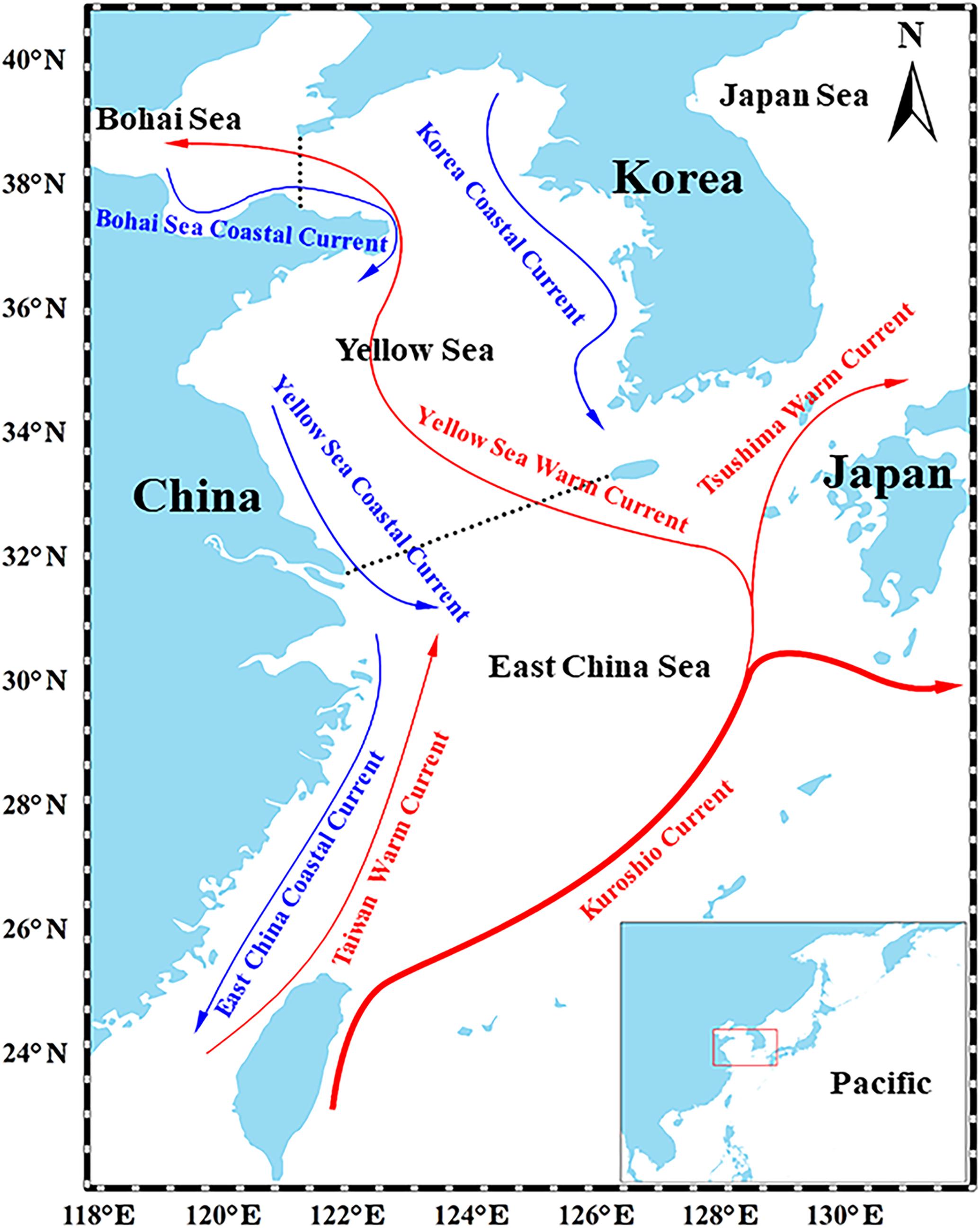
Figure 1. Map of the East China Continental Shelf Sea. Red and blue lines represent the primary warm currents and cold currents that affect the YS, respectively. The panel at the bottom-right shows the location of the YS in the Northwest Pacific (Ma et al., 2018).
Ecological Indicators of Fish Community Structure
In this study, we used a series of selection criteria suggested in Otto et al. (2018a) to select candidate indicators. As fishery-independent data from research surveys are rare in the YS (e.g., Liang et al., 2020), we took advantage of the YS catch time-series data from 1960 to 2014 obtained through the Sea Around Us project1 (Pauly and Zeller, 2016) to derive ecological indicators. Catch data were summarized to species, genus, family, order, and class. All species were classified into four functional groups, namely the large predatory, small pelagic, demersal, and invertebrate groups according to their trophic levels, biological characteristics, and previous studies (Tian et al., 2006, 2013). All the species were also categorized into three thermal groups, namely warm-water, temperate-water, and cold-water groups according to their optimal temperature (Ma et al., 2019). Based on the catch data of the corresponding groups, we calculated 22 IFCSs that represent the YS large marine ecosystem (Table 1). These 22 IFCSs include 5 indicators based on all species (termed “total-IFCSs”), 11 indicators based on functional groups (“functional-IFCSs”) and six indicators based on thermal groups (“thermal-IFCSs”). Specifically, total-IFCSs include total catch (ToC), the mean trophic level (MTL), the mean temperature of catch (MTC), Whilm species diversity (H″), and McNaughton dominance (Dom). Functional-IFCSs contain catch of large predatory groups (LPC), catch of small pelagic groups (SPC), catch of demersal groups (DeC), catch of invertebrate groups (InC), the ratio of LPC to ToC (LPC/ToC), the ratio of SPC to ToC (SPC/ToC), the ratio of the ratio of DeC to ToC (DeC/ToC), the ratio of InC to ToC (InC/ToC), the ratio of DeC to SPC (DeC/SPC), the ratio of LPC to SPC (LPC/SPC), and functional evenness based on functional groups (F-J′FD). Thermal-IFCSs consist of catch of warm-water groups (WWC), catch of cold-water groups (CWC), the ratio of WWC to ToC (WWC/ToC), the ratio of CWC to ToC (CWC/ToC), the ratio of WWC to CWC (WWC/CWC), and functional evenness based on thermal groups (T-J′FD).
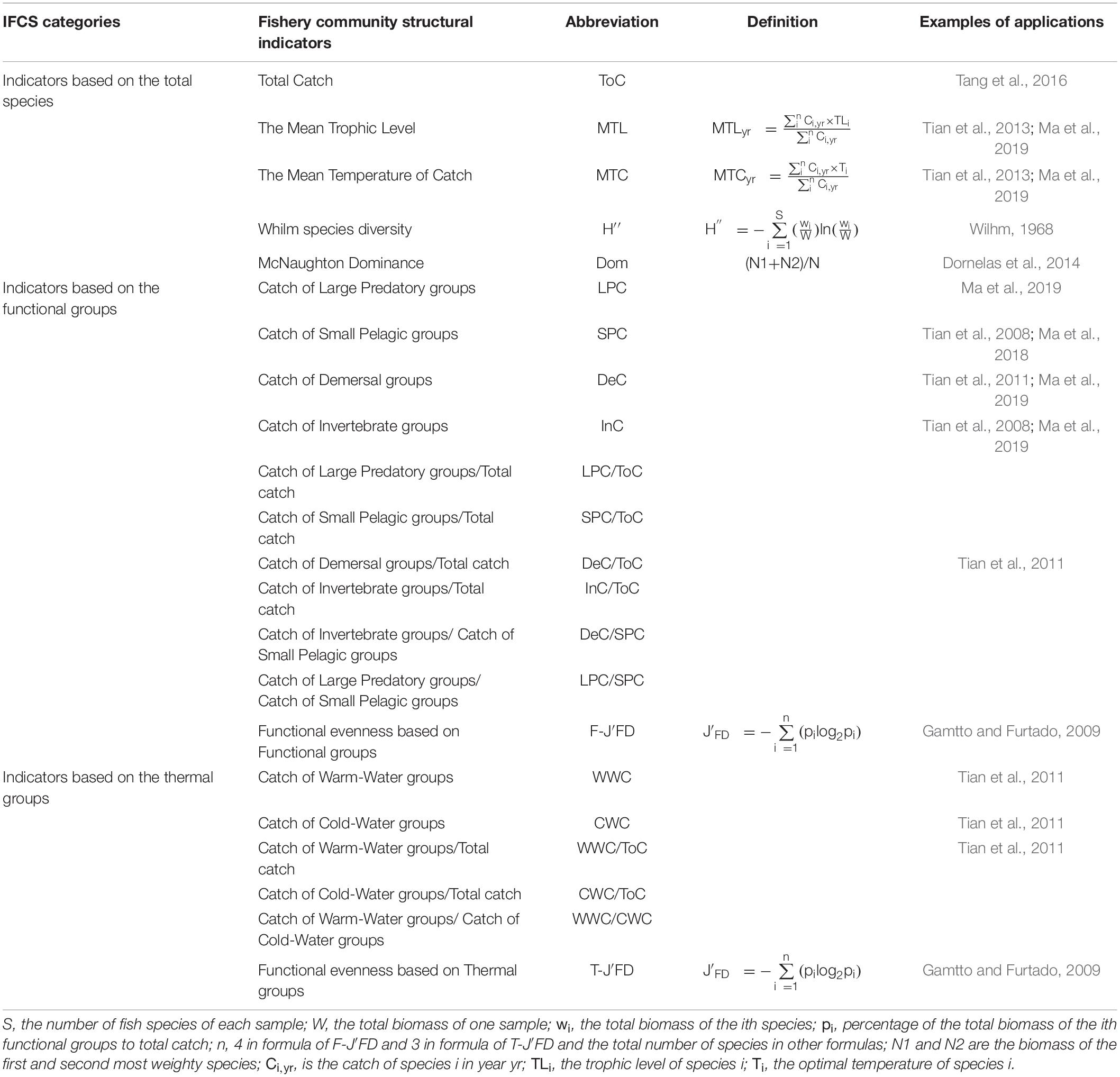
Table 1. List of fishery community structural indicators tested for YS.
Prior to the calculation of each indicator, multiple imputation with Bayesian linear regression techniques (Buuren and Groothuis-Oudshoorn, 2011) was used to fill the missing values of the catch data in the YS (1.43%). Multiple imputation was performed using the packages “mice” within the “R” statistical and programming environment (R Core Team, 2019), with each imputed value derived from five iterations and each iteration consisting of 100 imputations.
Pressure Variables
A total of eight large-scale climate indices were tested for their effects on all IFCSs, including the Pacific Decadal Oscillation (PDO), North Pacific Gyre Oscillation (NPGO), Arctic Oscillation Index (AOI), Pacific-North America Index (PNA), North Pacific Index (NPI), Southern Oscillation Index (SOI), Asian Monsoon Index (MOI), and Sea Surface Temperature in Nino 4 Region (Nino 4). Descriptions, data sources, and spatial-temporal resolutions of these climate indices are provided in Supplementary Table 1. These climatic variables are well documented and largely associate with the ecosystems and their fish communities in the North Pacific (Boeing and Duffy-Anderson, 2008; Ceballos et al., 2009; Litzow et al., 2014; Kidwell et al., 2017).
In addition to the large-scale climate indices, seven well-documented environmental indices in the YS, including sea surface temperature (SST), sea surface salinity (SSS), sea level pressure (SLP), scalar wind (SW), wind direction (WD), air temperature (AT), and precipitable water content (PWC), were also selected to represent regional environmental conditions (Cui and Zorita, 1998; Park et al., 2015; Zheng et al., 2015) and to test the responses of IFCSs. More details on these environmental indices are provided in Supplementary Table 1.
Anthropogenic pressures in the YS were approximated by fishing efforts (FE) in the following statistical analyses to understand the responses of IFCSs. Engine power data for the total number of Chinese marine fishing boats in the YS were derived from Chinese Fishery Statistics from 1960 to 2014 to represent fishing efforts (Zhao et al., 2015). Due to the lack of other accurate fishing effort indices for specific species/groups, we assumed fishing efforts were the same across all fish species.
Indicator-Testing Framework
The indicator-testing framework of Otto et al. (2018a) was used to assess the performances of IFCSs and further choose a set of complementary and robust indicators for representing the FCS in the YS. Before conducting statistical analyses, all the 22 IFCSs were standardized by zero-mean normalization. All calculations were done using the package “INDperform” (Otto et al., 2018b) within the R environment (R Core Team, 2019). The indicator-testing framework, combined with score criteria (Supplementary Table 2), is a seven-step process with the first five steps being used to validate and quantify the performances of IFCSs in their responses to pressures (Supplementary Table 1).
Specifically, Step 1 identifies indicators’ trends and links to the score criterion 1. Generalized additive models (GAMs; Hastie and Tibshirani, 1990) are applied to model the long-term changes of IFCSs in response to one pressure (explanatory variable) at a time. When there are significant temporal auto-correlation in residuals, the alternative Generalized Additive Mixed Models (GAMMs) are used. A score of 1 is given if an IFCS shows a significant trend, otherwise, score 0. Step 2 identifies the responses of IFCSs to pressures and links to sub-criterion 2.1 and the first two sub-criteria of criterion 3. Step 3 measures the robustness of an IFCS in relation to one specific pressure based on the degree of fit for the last 3 years between predictions from the model using the training dataset (i.e., excluding the last 3 years) and the test dataset (i.e., the last 3 years). The score of sub-criterion 3.3 is according to the value of the normalized root mean square error (NRMSE) on the test dataset.
In the case of non-linear responses of IFCSs to pressures, the method of finite differences (Trenkel and Rochet, 2009) is used to test the first derivative of the smoothing function, representing the instantaneous change rate of IFCSs to that of the pressures in Step 4. Confidence intervals (CI) of the first derivative are generated by carrying out a conditional bootstrap by resampling from the GAM (or GAMM) residuals. The IFCSs’ responses to changes in pressures are not considered to be statistically significant when zero is contained within the CI of the first derivative. Subsequent scoring sub-criterion 2.2 was done via counting the proportion of points inside the CI. In Step 5, the threshold GAM (TGAM; Ciannelli et al., 2004) is used to detect interactions between pressures corresponding to criterion 3.4. A zero score for sub-criterion 3.4 is given if interactions with other pressure(s) are detected. The IFCS with summed scores of sensitivity and robustness > 50% of maximum score is considered to have good performances in their responses to pressures.
In Step 6, Nightingale rose diagrams are used to visualize the overall performance of the IFCSs. Finally, in Step 7, a hierarchical group-average cluster analysis (Legendre and Legendre, 1998) is carried out based on the sub-criteria scores of sensitivity (criterion 2), robustness (criterion 3), and the other two criteria (criteria 1 and 4) to recognize redundant IFCSs. Then a final indicator suite is identified based on the following criteria (Otto et al., 2018a): (1) responsiveness to at least one pressure, (2) non-redundancy, i.e., the IFCSs is not grouped with other IFCSs at the lowest level in the cluster analysis, or having higher scores in sensitivity and robustness than their redundant counterpart in the same cluster, (3) good performance (the sum scores of sensitivity and robustness >50% of the maximum score), and (4) complement, i.e., the IFCS covers the full types of pressures together with other IFCSs.
State Space Approaches and Regime Shift Detection
For the final indicator suite, two state-space approaches were applied to analyze the temporal dynamics of the FCS. One approach is to calculate the Euclidean distance between each year and a reference year (de Berg et al., 2008), and the referent year is set as the initial year 1960 in this study. The other one is the convex hull method (Swenson, 2014), in which we first calculated the convex hull for a reference period (1960–1964) based on the first two axes obtained from a Principal Component Analysis (PCA), then calculated the convex hull of the current period (2010–2014) to determine whether there was overlap between the two closed spaces.
The PCA was applied to identify the most important patterns of common variability in the FCS. Only the first two PCs (PC1 and PC2) for the IFCSs were retained for representing the most important modes of variability in the final indicator suite. The sequential t-test analysis of regime shift (STARS; Rodionov, 2004; Rodionov and Overland, 2005) was then used to detect trends and regime shifts in the derived PCs. STARS was written in Visual Basic for Application (VBA) for Microsoft Excel and was available at www.BeringClimate.noaa.gov. To assist visualizing the trends in the time series of PCs, the cumulative sum (CuSum) was calculated by a simple addition of a datum to the sum of all previous data points (Beamish et al., 1999; Tian et al., 2004). In addition, because the results of STARS are easily affected by the cut-off length, sensitivity analysis on the cut-off length was also conducted. Specifically, the STARS was run successively with the value of the cut-off length changing from 10 to 20 with an increment of 0.01, then the frequencies of time nodes being selected as potential regime shifts were summed to identified the time node with the highest frequency as the regime shift.
Results
The Performances of the IFCSs in the YS
The IFCSs in different categories tended to have differing responses to pressures (Table 2). All total-IFCSs were insensitive to climate indices while being highly affected by fishing efforts. The functional-IFCSs responded selectively to fishing efforts but not to environmental indices showing primarily low performances. By contrast, the thermal-IFCSs, especially the index T-J′FD, showed high sensitivity in their responses to all three types of pressures. All IFCSs responded significantly to at least one pressure except Dom and H″ (Table 2) with only H″ showing no trend (Supplementary Figure 1). However, none of the IFCSs showed a direct response to the regional environmental index (WD) and three large-scale climate indices (NPI, MOI, and Nino 4). Therefore, these four pressure indices were excluded from the subsequent analysis. Among the 22 IFCSs that responded to one or more pressures, half showed good performances in their responses to pressures (Table 2). In terms of sensitivity, a majority of IFCSs (18 out of 22) showed good performance with scores >50%. By contrast, none of the IFCSs scored more than 50% of the total score in terms of robustness, which resulted in weak performance for many IFCSs (Table 2). Among all IFCSs, the indicators of LPC/ToC, CWC, and WWC/ToC showed significant linear responses to all their pressures. In contrast, relevant non-linear responses to all their significant pressures were found for SPC/ToC, DeC/ToC, InC/ToC, DeC/SPC, LPC/SPC, and F-J′FD (Table 2 and Supplementary Figure 2). Another striking feature across all IFCSs was that one or more threshold interactions were found for every IFCS (Supplementary Figure 2). For example with T-J′FD, there was a threshold interaction with PNA: under lower PNA conditions (<0.97) the negative effect of fishing efforts remained constant and linear, but under higher PNA conditions (>0.97) there were no significant responses (Supplementary Figure 2).
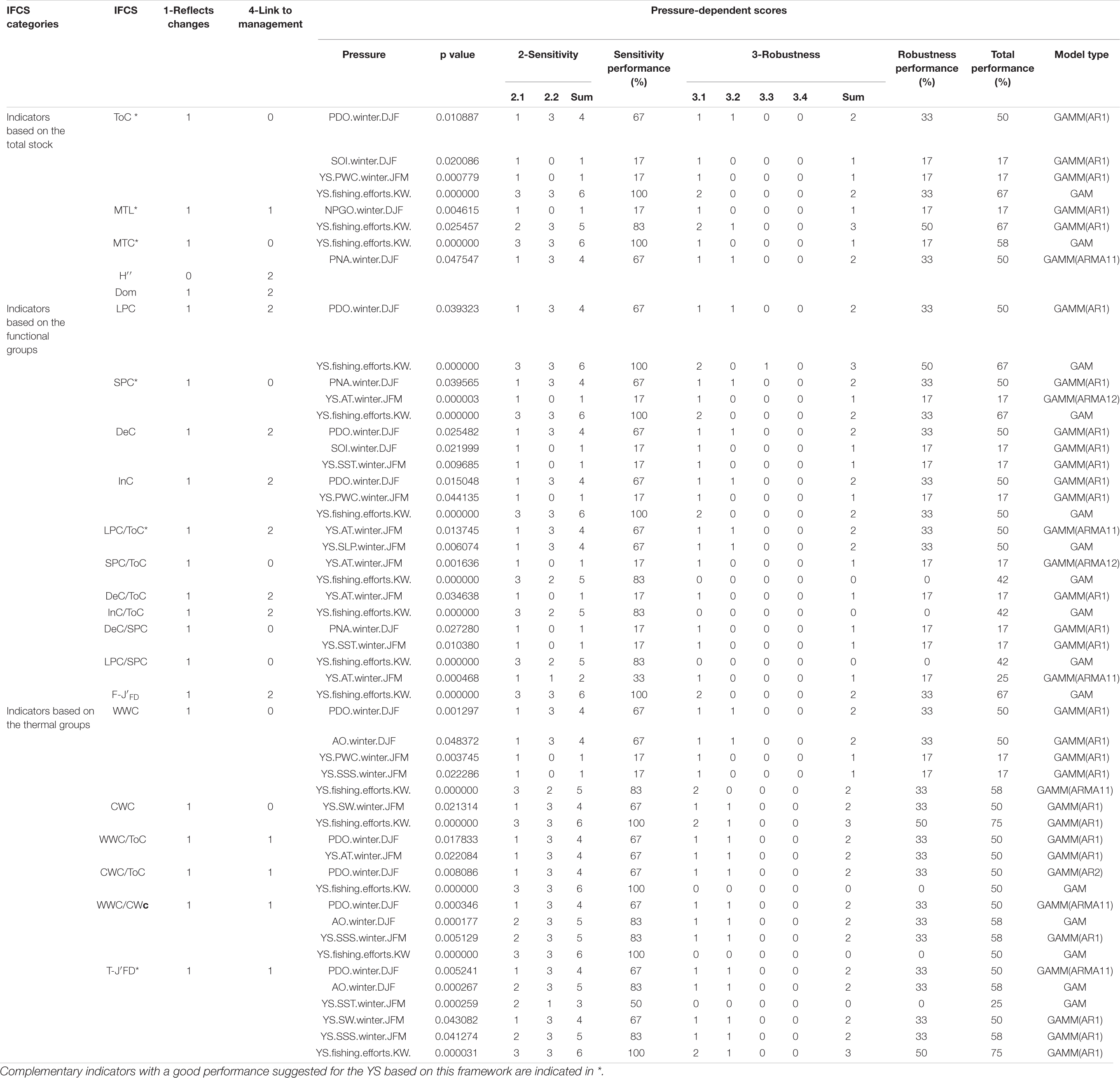
Table 2. Overview of performance scores of fishery ecosystem structure indicators for each criterion in the YS.
Indicator Suite for the YS
Based on the performances of the 22 IFCSs and the need to reduce redundancies found amongst the 22 IFCSs (Figure 2), we identified two combinations (Combinations I and II) with each consisting of five indicators. Either combination can be considered as a final robust indicator suite. Combination I comprised one thermal-IFCS (T-J′FD), one functional-IFCS (LPC/ToC) and three total-IFCS (ToC, MTL, MTC). Combination II consisted of one thermal-IFCS (T-J′FD), two functional-IFCSs (LPC/ToC, SPC) and two total-IFCSs (ToC, MTL). Together, these IFCSs would allow the evaluation of impacts from large-scale climatic and regional environmental changes as well as fishing effort. The total-IFCSs are suitable for detecting the impacts of fishing efforts and climate variability with ToC and MTC showing strong responses to PDO and PNA, respectively. By contrast, MTL showed a specific response to fishing efforts. As a synthetic indicator of thermal-IFCSs, T-J′FD showed a strong and robust response to climate indices (i.e., PDO and AO), environmental indices (i.e., SSS and SW), as well as fishing efforts. For the functional-IFCSs, LPC/ToC only responded to environmental indices, but not to fishing efforts and climate indices, while SPC showed strong response to fishing efforts and two climatic indices (Table 2).
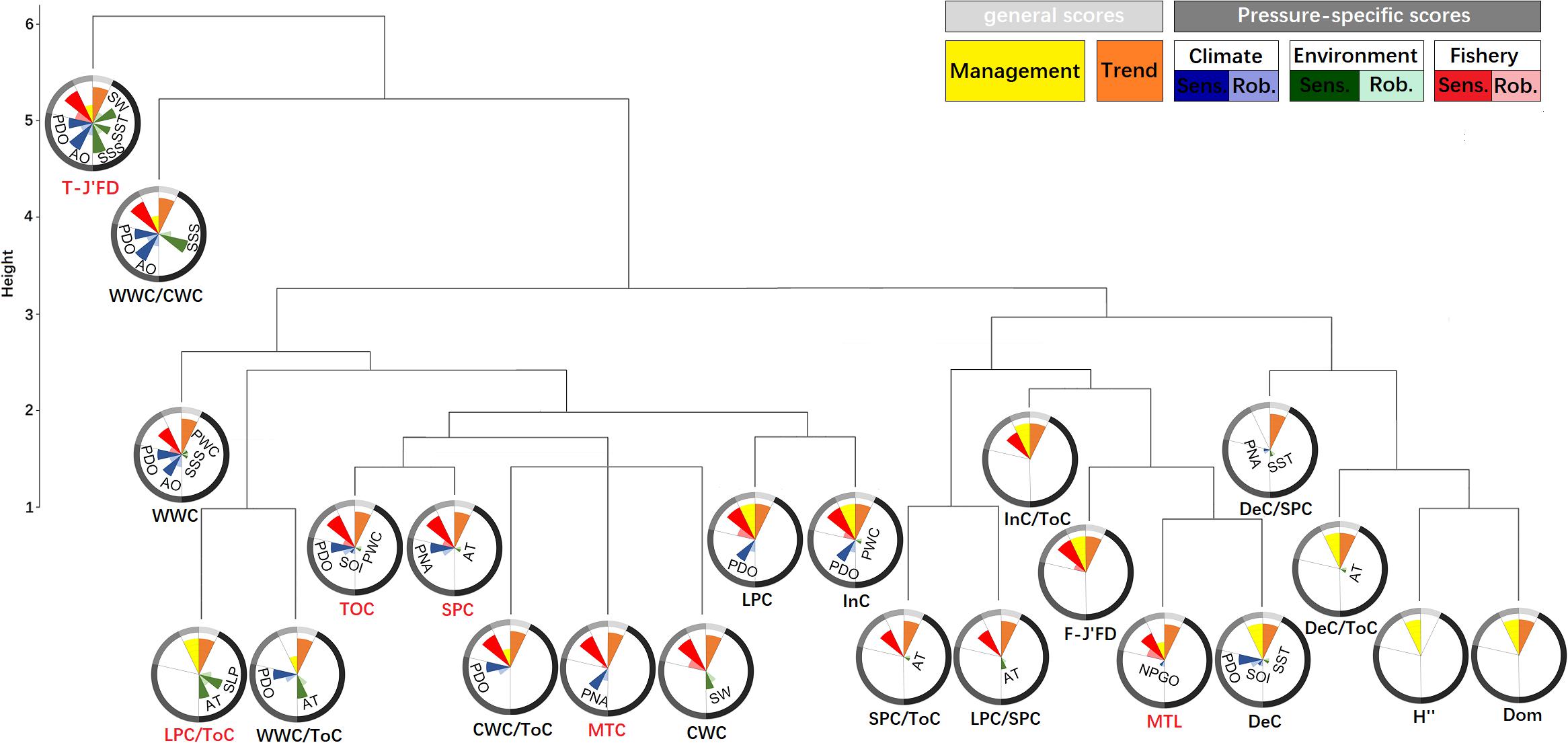
Figure 2. Dendrograms from hierarchical cluster analyses of fishery ecological structure indicators of the YS. For each indicator nightingale rose diagrams are displayed to visualize their performance scores. Sensitivity (opaque color) and robustness (transparent color) scores are shown individually for each significant pressure. The length of the bars represents the percentage of achieved score from the maximum with the boundary line indicating the 100%.
The Dynamics of the FCS in the YS
Both robust combinations of IFCSs showed that the FCS in the YS has departed substantially from their reference state (Figure 3). Although the Euclidean distance scalar of combination I suggested the YS returning to the earlier state after 2000 (Figure 3A), the state approach based on the PCA indicated clearly that the last five years of the current period are outside the reference domain in terms of PC1 dimensions (Figure 3B). There were also true for Combination II (Figures 3C,D). The first two PCs accounted for 85.5 and 88.5% of the final IFCSs variances for the Combinations I and II, respectively (Figures 3B,D).
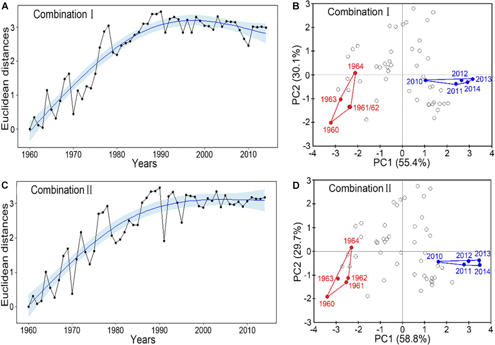
Figure 3. Evaluation of the current fishery community structural state based on the final indicator suite. Panels (A,C) show the time trajectories of Euclidean distance in indicator state space from arbitrary reference year 1960, including a fitted trend with 95% confidence interval. The distance was calculated as the square root of the sum of squared distances between each standardized indicator value in a specific year and its reference value. Panels (B,D) show the location of the last 5 years in the time series (blue) in the 2-dimensional principal component (1st and 2nd) space in comparison to the state domain of the reference period 1960–1964 (red). Combination I consists of ToC, LPC/ToC, MTL, MTC, T-J′FD; combination II consists of ToC, LPC/ToC, MTL, SPC, T-J′FD.
For Combination I, step-like changes occurred in 1971/72, 1985/86, and 2003/04 for PC1 and 1976/77 and 1990/91 for PC2 (Figures 4, 5); similar results were found in Combination II (Supplementary Figures 3, 4). As all five robust IFCSs have high loadings on one or both PCs (Figure 6 and Supplementary Figure 5), this can be interpreted as a deviation from the reference period in all components of the FCS represented by the suites with values of ToC and MTC (alternatively SPC) being lower while MTL, LPC/ToC and particularly T-J′FD being higher during the reference period (Figure 6 and Supplementary Figures 1, 5).
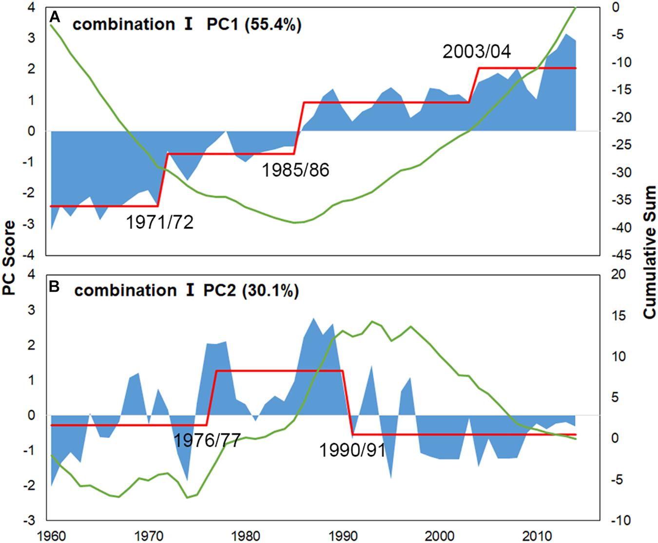
Figure 4. PC scores for the final indicator suite (consist of ToC, LPC/ToC, MTL, MTC, T-J′FD). Blue areas represent scores, green lines denote cumulative sums for scores and red lines represent regime means detected by STARTS.
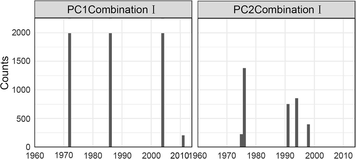
Figure 5. Sensitivity results of STARTS to cut-off length for the final indicator suite (consist of ToC, LPC/ToC, MTL, MTC, T-J′FD). Gray bars represent time nodes with considerable probability of regime shifts.
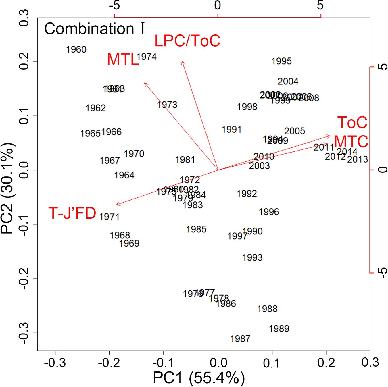
Figure 6. Results of the standardized principal component analysis (PCA) using the final indicator suite (consist of ToC, LPC/ToC, MTL, MTC, T-J′FD). Red lines describing the indicator loadings on the first and second principal components (PC).
Discussion
Performance of IFCSs in the YS
In general, the first five steps of the indicator-testing framework have indicated that the majority of the 22 IFCSs of the YS showed good performances in terms of their sensitivity to pressures, but weak performances in terms of robustness. Regime shifts of marine fish community are frequent occurrences accompanying climate regime shifts (Tian et al., 2006, 2008; Litzow and Ciannelli, 2007; Möllmann and Diekmann, 2012), and such abrupt changes can only be explained by non-linear state changes in response to sudden changes in pressures (Petersen et al., 2008; Fu et al., 2015). However, the IFCS-pressure relationships in our study were largely linear (27 of the 51 significant pressure responses), which contribute to low scores in one of the robustness criteria i.e., Criterion 3.2. Such linear relationships may partly be due to the standardization of data as suggested by Otto et al. (2018a). In addition, all IFCSs that had significant responses to at least one pressure were found to have one or more threshold interactions, which was a primary reason for the low scores in the robustness aspect. Threshold interactions are often used to test non-additive interactions between two types of pressures, which are important for assessing population dynamics (Ciannelli et al., 2004). Threshold responses in potential interactions between pressures provide guidance for potential reference points for fisheries management (Fu et al., 2019). From a conservation perspective, a threshold may represent a risk point where the risk of species loss increases sharply (Toms and Villard, 2015). For example, overfishing cod (Gadus morhua) may change the dynamics of predation-prey relationships between cod and zooplankton, and thus damage the population dynamics of cod (Casini et al., 2009). Therefore, thresholds may offer critical insight and useful guidelines when developing ecosystem-based conservation objectives (Samhouri et al., 2010). From this point, IFCSs that show threshold interactions in their responses to pressures proved their utility for EBFM.
Although 22 IFCSs were considered from different population perspectives, only five indicators were contained in the final indicator suite which were identified based on the performance of each IFCS and the need to reduce redundancies, which were ubiquitous among the IFCSs derived from the unitary data (i.e., only catch data). The five indicators within Combination I, the thermal-IFCS T-J′FD jointly with the functional-IFCS LPC/ToC and the total-IFCSs MTL, ToC and MTC, would allow the evaluation of management measures related to all significant pressures. In particular, the introduction of comprehensive indices MTL and MTC helped improve the data dimension (going beyond catch data only) by incorporating biological characteristics of fish. The MTL and MTC indicators have been widely used in related research to reflect the trophic level and optimal temperature of species, respectively (Tsikliras and Stergiou, 2014; Hermida and Delgado, 2016). In Combination II, SPC was included in the place of MTC as both of them responded to the same pressure PNA with the same performance. Although the results of the two combinations are similar, we focused on Combination I in our result presentation and discussion as the final indicator suite to reflect long-term trajectory of the FCS in the YS as the indicator MTC incorporates biological characteristics of fish while SPC is unitary (based on catch data only). To facilitate the move towards EBFM in the YS by employing and evaluating more comprehensive ecological indicators in terms of their responses to management-related key pressures, we advocate continuous and consistent research surveys to collect pluralistic data, such as length (Large et al., 2013), abundance (Shannon et al., 2009), and age structure (Shin et al., 2010), which are largely lacking in the YS.
In previous studies, LPC (Myers and Worm, 2005) and DeC (Newman et al., 2015, 2016) were found most suitable and subsequently implemented in fisheries management. However, these indicators did not perform necessarily best for the study period (1960–2014) in the YS. Specifically, LPC had high redundancy with ToC and T-J′FD within the final indicator suit in terms of its response to fishing efforts and PDO. In addition, the relationship between DeC and its significant pressures was less robust than LPC/ToC. Such results demonstrate that not all indicators are suitable for fisheries management in all ecosystems, even if they are sensitive in their responses to relevant pressures. We would encourage that the evaluation of indicator performances is done on an ecosystem-specific basis because of the unique characterizes of an ecosystem and the diverse fishery exploitation history (Fu et al., 2019).
Furthermore, the final indicator suite would not be applicable for evaluating the impact of four pressures (i.e., WD, NPI, MOI, Nino 4) as all IFCSs were not found significant in their response to them. Therefore, more comprehensive ecological indicators are needed to evaluate the impacts of these four pressures, and the performance of candidate indicators should be validated before they can be used for assessing ecosystem dynamics and guiding fisheries management.
Optimal Indicators for Reflecting Relative Pressures
Among multiple pressures that impact marine ecosystems, climate change plays one of the most important roles (Barange et al., 2014; Kirkman et al., 2015; Kadin et al., 2019). For instance, climate change was found to be important factor in evaluating the responses of small pelagic fish, an important functional group in marine fish communities, to fishing pressure and decadal variations (Tian et al., 2013; Ma et al., 2018). However, climate change was not identified as important in our study. The SPC was shown to have significant response only to one climate index (i.e., PNA) with weak robustness contrary to previous studies. Moreover, some indicators such as MTC commonly used to reflect climate changes (Tsikliras and Stergiou, 2014) showed no sensitivity to any climate indices. As a whole, 13 of the 22 IFCSs tested significant in their response to one or more climate indices (Table 2). The response mechanism of fish communities to climate change is complex. Climate change may impact the dynamics of marine ecosystems via complex “Atmosphere-ocean-ecosystem” processes (Ma et al., 2019), causing increases in sea water temperature, which further alters reproduction effectiveness (Palomera et al., 2007), survival (Martins et al., 2012), distributional shifts along latitudinal and depth gradients (Perry et al., 2005; Simpson et al., 2011), and other behavioral variations (Goniea et al., 2006; Audzijonyte et al., 2020). It is generally acknowledged that the responses of marine fish communities to climate change can vary among regions (Barange et al., 2014; Guenette et al., 2014), resulting in regional specificity in the performances of IFCSs. Again, our results advocate that it is imperative to validate indicators in different ecosystems before using them in management decisions, as suggested by Östman et al. (2017).
In general, IFCSs have different sensitivity in their responses to different environment variables, and significant responses to regional environment variables mainly occurred in functional-IFCSs and thermal-IFCSs (Table 2). Regional environmental conditions affect FCS directly by limiting the distribution of organisms within their tolerance range or indirectly by altering species interactions (Ochoa-Hueso, 2016). For example, Ocean warming has modified marine biology community structure by increasing biodiversity and miniaturizing the plankton ecosystem, which negatively affects demersal Atlantic cod (Beaugrand et al., 2010). Younger copepodites have strong sensitivity to midwater temperature in spring and summer, while there is a strong positive correlation between females and older copepodites and deep water salinity from spring till autumn (Otto et al., 2020). Moreover, potential threshold interactions among pressures can also alter the shape of the relationships between responses and pressures (Pang et al., 2018). Therefore, considering species compositions in specific food webs is important when employing ecosystem indicators in the evaluation of pressures and management measures.
Marine ecosystems are affected by multiple human pressures (Halpern et al., 2008). Early fisheries studies around the world have provided sufficient proof that several fish groups have declined markedly in population sizes even resulting in local extinction of some vulnerable species, both as target and by-catch species (Stevens et al., 2000). Continuous overfishing also resulted in miniaturization of important commercial species and reconstruction of total fish communities (Conover et al., 2005). Consequently, fishery-based ecosystem indicators are commonly sensitive to fishing efforts (Gascuel et al., 2016). Although we only used engine power data as proxies for the total number of Chinese marine fishing boats in the YS, our results showed that 15 of 22 IFCSs were sensitive to fishing efforts. In particular, the indicators MTL, LPC and T-J′FD were found to have highest sensitivity and robustness compared with other indicators within the final indicator suite. In contrast, the indicators DeC, LPC/ToC, DeC/ToC, DeC/SPC, WWC/ToC showed no significant responses to fishing efforts. The responses of indicators to fishing can be altered by species interactions. For example, small pelagic forage fish often increases apparently accompanying the decline of large predatory fish due to overfishing, which in turn results in the decrease of the biomass of zooplankton and phytoplankton (Frank et al., 2005). Therefore, Using fishing mortality of specific species is optimal when assessing the influences of fishing. In future studies, we intend to introduce more accurate mortality rate of specific species as proxies for anthropogenic pressures.
Long-Term Changes of the FCS in the YS
Combining the scores of IFCSs with the hierarchical group-average cluster analysis, we identified five IFCSs forming a final indicator suite as a proxy for the FCS in the YS. Although only 5 of 22 IFCSs were retained in the final indicator suite and the basic data were simple, our analysis sheds light on the dynamics of the FCS in the YS, proving sufficiency of the five IFCSs in the final indicator suite to represent synthetical information on fish community dynamics. Regime shifts detected in the mid-1970s and the early 1990s (Figure 4) coincided with the climate regime shifts based on the integrated trend analysis using many climate indices, while detected shifts in the final indicator suite in the mid-1980s coincided with the regime shifts of regional environment variables (Ma et al., 2019). The shift detected in the early 1970s was not accompanied by any types of pressures, which may result from the fact that no indicators tested in this study were sensitive to the four pressures (i.e., WD, NPI, MOI, Nino 4), indicating that the final indicator suite was unsuitable for evaluating the impacts of these four pressures.
Both state space approaches indicated that the status of the FCS of the YS deviated obviously from the reference year, despite some level of returning to the earlier state after 2000 (Figure 3A). There is ample evidence that the dynamics of the FCS in the YS synchronized with other regions in the world based on more relevant indices (Perry et al., 2005; Atkinson et al., 2011; Kirkman et al., 2015). The long-term trajectory of the final indicators suite in the study period derived from Euclidean distances analysis was highly consistent with fishing effort in the YS, suggesting that the final indicators suite could reflect fishing efforts appropriately. The PCA convex hull analysis for the final indicator suite showed that SPC contributed most to the observed changes in the IFCSs state space, reflecting the declines of large predatory fish biomass in global ocean (Ransom and Worm, 2003) and also reflecting the increases of small pelagic fish because of reduced predation mortality by large predatory fish (Cury et al., 2000). Moreover, the fluctuation of small pelagic fishes varied with species in the YS (Ma et al., 2018), implying that the increases of small pelagic fish were not only due to the reduction of predators. Therefore, our results also indirectly indicated that environmental conditions may have changed compared to the reference period as small pelagic fish are highly dependent on external environmental conditions (Merino et al., 2010). Such dynamics are also reflected in the decline of the mean trophic level (Zhang et al., 2007), supported by our result concerning MTL. In combination I, MTC plays the most important role, reflecting that global warming is more friendly to warm-water species than cold-water species (Almodóvar et al., 2012; O’Gorman et al., 2016). Global warming caused water temperature range to gradually fluctuate away from the niche of cold-water species, which is adverse to cold-water species but advantageous to warm-water species. Such results were also reflected in another important indicator, i.e., T-J′FD, contributing to the observed changes. Its long-term changes indicated that the resources distribution of three thermal groups trends more evenness with CWC/ToC gradually declining while WWC/ToC generally increasing within the observation period (Supplementary Figure 1). ToC ranked second in its contribution to changes in the IFCS state space, reflecting the rapid increasing of total catch (FAO, 2016).
As the YS ecosystem is continually facing impacts from overfishing and climate change, resulting in serious declines of fishery resources and miniaturization, it is imperative to move towards EBFM. The great change of the FCS in the YS has been proven by our final indicator suite, which can subsequently be used as an effective tool in ecosystem monitoring to reach management targets (Levin et al., 2009). In particular, the increase of SPC has been identified as one of the most outstanding changes of the FCS in the YS. Therefore, we advocate that the management objective of increasing size of fish should be include in the EBFM in the YS, which can potentially be achieved by enlarging mesh size.
Conclusion
In this study, we use a quantitative and flexible framework to verify the performance of IFCSs that represent various aspects of the FCS in the YS. As different regions have different management objectives, we used nightingale rose diagrams to exhibit the performance of IFCSs in relation to pressure management visually. Five indicators, ToC, MTL, LPC/ToC, MTC (or alternatively SPC) and T-J′FD, were determined to form the final indicator suite as a proxy for the FCS in the YS. The five indicators are suitable to detect different pressures with LPC/ToC to SLP and AT; ToC to PWC and SOI; MTC to NPGO; MTC (and SPC) to PNA; T-J′FD to SW, SST, AO and SSS, respectively, while PDO can be detected by both ToC and T-J′FD. Fishing effort can be detected by five indicators of the final indicator suite except LPC/ToC. Based on the final indicator suite, we found the FCS in the YS is deviate distinctly from an earlier reference period, suggesting the impact of over-fishing. The indicator-testing framework has been demonstrated to be applicable to the FCS in the YS. Future fishery and ecosystem management should use the indicator-testing framework for selecting suites of complementary indicators under given management objectives.
Data Availability Statement
The original contributions presented in the study are included in the article/Supplementary Material, further inquiries can be directed to the corresponding authors.
Author Contributions
YL performed the data analyses and wrote the manuscript. CF participated in data analysis. SM conceived the idea for the study. YT and YL helped design the study, and critically revised the manuscript. JL, PS, and ZY edited the manuscript. All authors listed have made a direct and substantial contribution to this work, gave final approval for publication, and agreed to be held accountable for the work performed therein.
Funding
This study was supported by the National Key R&D Program of China (No. 2018YFD0900902), Shandong Key R&D Program (No. 2019GHY112014), and the National Natural Science Foundation of China (NSFC) (Grant Nos. 41930534, 41861134037, and 41876177).
Conflict of Interest
The authors declare that the research was conducted in the absence of any commercial or financial relationships that could be construed as a potential conflict of interest.
Supplementary Material
The Supplementary Material for this article can be found online at: https://www.frontiersin.org/articles/10.3389/fmars.2021.646733/full#supplementary-material
Footnotes
References
Almodóvar, A., Nicola, G. G., Ayllón, D., and Elvira, B. (2012). Global warming threatens the persistence of Mediterranean brown trout. Glob. Chang. Biol. 18, 1549–1560. doi: 10.1111/j.1365-2486.2011.02608.x
Atkinson, L. J., Leslie, R. W., Field, J. G., and Jarre, A. (2011). Changes in demersal fish assemblages on the west coast of South Africa, 1986–2009. Afr. J. Mar. Sci. 33, 157–170. doi: 10.2989/1814232X.2011.572378
Audzijonyte, A., Richards, S. A., Stuart-Smith, R. D., Pecl, G., Edgar, G. J., Barrett, N. S., et al. (2020). Fish body sizes change with temperature but not all species shrink with warming. Nat. Ecol. Evol. 4, 809–814. doi: 10.1038/s41559-020-1171-0
Barange, M., Merino, G., Blanchard, J. L., Scholtens, J., Harle, J., Allison, E. H., et al. (2014). Impacts of climate change on marine ecosystem production in societies dependent on fisheries. Nat. Clim. Chang. 4, 211–216. doi: 10.1038/nclimate2119
Beamish, R. J., Noakes, D. J., McFarlane, G. A., Klyashtorin, L., Ivanov, V. V., and Kurashov, V. (1999). The regime concept and natural trends in the production of Pacific salmon. Can. J. Fish. Aquat. Sci. 56, 516–526. doi: 10.1139/f98-200
Beaugrand, G., Edwards, M., and Legendre, L. (2010). Marine biodiversity, ecosystem functioning and the carbon cycles. Proc. Natl. Acad. Sci. U.S.A. 107, 10120–10124. doi: 10.1073/pnas.0913855107
Bhathal, B., and Pauly, D. (2008). ‘Fishing down marine food webs’ and spatial expansion of coastal fisheries in India, 1950–2000. Fish. Res. 91, 26–34. doi: 10.1016/j.fishres.2007.10.022
Bjørnstad, O. N., and Grenfell, B. T. (2001). Noisy clockwork: time series analysis of population fluctuations in animals. Science 293, 638–643. doi: 10.1126/science.1062226
Boeing, W. J., and Duffy-Anderson, J. T. (2008). Ichthyoplankton dynamics and biodiversity in the Gulf of Alaska: responses to environmental change. Ecol. Indic. 8, 292–302. doi: 10.1016/j.ecolind.2007.03.002
Burgess, M. G., Giacomini, H. C., Szuwalski, C. S., Costello, C., and Gaines, S. D. (2017). Describing ecosystem contexts with singlr-species models: a theoretical synthesis for fisheries. Fish Fish. 18, 264–284. doi: 10.1111/faf.12179
Buuren, S. V., and Groothuis-Oudshoorn, K. (2011). Mice: multivariate imputation by chained equations in R. J. Stat. Softw. 45, 1–68.
Cai, R., Tan, H., and Qi, Q. (2016). Impacts of and adaptation to inter-decadal marine climate change in coastal China seas. Int. J. Climatol. 36, 3770–3780. doi: 10.1002/joc.4591
Casini, M., Hjelm, J., Molinero, J. C., Lövgren, J., Cardinale, M., Bartolino, V., et al. (2009). Trophic cascades promote threshold-like shifts in pelagic marine ecosystems. Proc. Natl. Acad. Sci. U.S.A. 106, 197–202. doi: 10.1073/pnas.0806649105
Ceballos, L. I., Lorenzo, E. D., Hoyos, C. D., Schneider, N., and Taguchi, B. (2009). North Pacific gyre oscillation synchronizes climate fluctuations in the eastern and western boundary systems∗. J. Clim. 22, 5163–5174. doi: 10.1175/2009JCLI2848.1
Chen, C. (2004). Ammodytes personatus resources in the Yellow Sea and its sustainable utilization. J. Fish. China 28, 603–607. (in Chinese),Google Scholar
Ciannelli, L., Chan, K. S., Bailey, K. M., and Stenseth, N. C. (2004). Nonadditive effects of the environment on the survival of a large marine fish population. Ecology 85, 3418–3427. doi: 10.1890/03-0755
Conover, D. O., Arnott, S. A., Walsh, M. R., and Munch, S. B. (2005). Darwinian fishery science: lessons from the Atlantic silverside (Menidia menidia). Can. J. Fish. Aquat. Sci. 62, 730–737. doi: 10.1139/F05-069
Cui, M., and Zorita, E. (1998). Analysis of the sea-level variability along the Chinese coast and estimation of the impact of a CO2-perturbed atmospheric circulation. Tellus A 50, 333–347. doi: 10.3402/tellusa.v50i3.14530
Cury, P., Bakun, A., Crawford, R. J. M., Jarre, A., Qui?ones, R. A., Shannon, L. J., et al. (2000). Small pelagics in upwelling systems: patterns of interaction and structural changes in “wasp-waist” ecosystems. ICES J. Mar. Sci. 57, 603–618. doi: 10.1006/jmsc.2000.0712
de Berg, M., Cheong, O., van Kreveld, M., and Overmars, M. (2008). Computational Geometry- Algorithms and Applications. Berlin: Springer.
Dornelas, M., Gotelli, N. J., McGill, B., Shimadzu, H., Moyes, F., Sievers, C., et al. (2014). Assemblage time series reveal biodiversity change but not systematic loss. Science 344, 296–299. doi: 10.1126/science.1248484
Fabry, V. J., Seibel, B. A., Feely, R. A., and Orr, J. C. (2008). Impacts of ocean acidification on marine fauna and ecosystem processes. ICES J. Mar. Sci. 65, 414–432. doi: 10.1093/icesjms/fsn048
FAO (2016). The State of World Fisheries and Aquaculture 2016. Contributing to Food Security and Nutrition for all. Rome: FAO.
Frank, K. T., Petrie, B., Choi, J. S., and Leggett, W. C. (2005). Trophic cascades in a formerly cod-dominated ecosystem. Science 308, 1621–1623. doi: 10.1126/science.1113075
Fu, C., Large, S., Knight, B., Richardson, A. J., Bundy, A., Reygondeau, G., et al. (2015). Relationships among fisheries exploitation, environmental conditions, and ecological indicators across a series of marine ecosystems. J. Mar. Syst. 148, 101–111. doi: 10.1016/j.jmarsys.2015.01.004
Fu, C., Xu, Y., Bundy, A., Grüss, A., Coll, M., Heymans, J. J., et al. (2019). Making ecological indicators management ready: assessing the specificity, sensitivity, and threshold response of ecological indicators. Ecol. Indic. 105, 16–28. doi: 10.1016/j.ecolind.2019.05.055
Gamtto, S., and Furtado, R. (2009). Feeding diversity in macroinvertebrate communities: a contribution to estimate the ecological status in shallow waters. Ecol. Indic. 9, 1009–1019. doi: 10.1016/j.ecolind.2008.11.012
Garcia, S. M., and Cochrane, K. L. (2005). Ecosystem approach to fisheries: a review of implementation guidelines. ICES J. Mar. Sci. 62, 311–318. doi: 10.1016/j.icesjms.2004.12.003
Gascuel, D., Coll, M., Fox, C., Guénette, S., Guitton, J., Kenny, A., et al. (2016). Fishing impact and environmental status in European seas: a diagnosis from stock assessments and ecosystem indicators. Fish Fish. 17, 31–55. doi: 10.1111/faf.12090
Gissi, E., Manea, E., Mazaris, A. D., Fraschetti, S., Almpanidou, V., Bevilacqua, S., et al. (2021). A review of the combined effects of climate change and other local human stressors on the marine environment. Sci. Total Environ. 755:142564. doi: 10.1016/j.scitotenv.2020.142564
Goniea, T. M., Keefer, M. L., Bjormn, T. C., Peery, C. A., Bennett, D. H., and Stuehrenberg, L. C. (2006). Behavioral thermoregulation and slowed migration by adult fall chinook salmon in response to high Columbia River water temperatures. Trans. Am. Fish. Soc. 135, 408–419. doi: 10.1577/T04-113.1
Guenette, S., Araujo, J. N., and Bundy, A. (2014). Exploring the potential effects of climate change on the Western Scotian Shelf ecosystem, Canada. J. Mar. Syst. 134, 89–100. doi: 10.1016/j.jmarsys.2014.03.001
Halpern, B. S., Walbridge, S., Selkoe, K. A., Kappel, C. V., Micheli, F., D’agrosa, C., et al. (2008). A global map of human impact on marine ecosystems. Science 319, 948–952. doi: 10.1126/science.1149345
Hastie, T. J., and Tibshirani, R. J. (1990). Generalized Additive Models. Boca Raton, FL: Chapman Hall/CRC, doi: 10.1002/sim.4780110717
Hermida, M., and Delgado, J. (2016). High trophic level and low diversity: would madeira benefit from fishing down? Mar. Policy 73, 130–137. doi: 10.1016/j.marpol.2016.07.013
Hoegh-Guldberg, O., and Bruno, J. F. (2010). The impact of climate change on the World’s marine ecosystems. Science 328, 1523–1528. doi: 10.1126/science.1189930
Jennings, S. (2005). Indicator to support an ecosystem approach to fisheries. Fish Fish. 6, 212–232. doi: 10.1111/j.1467-2979.2005.00189.x
Jennings, S., and Kaiser, M. J. (1998). The effects of fishing on marine ecosystems. Adv. Mar. Biol. 34, 201–352. doi: 10.1016/S0065-2881(08)60212-6
Jin, X. S. (2003). Fishery biodiversity and community structure in the Yellow and Bohai Seas. Am. Fish. Soc. Symp. 38, 643–650.
Jørgensen, S. E., Nielsen, S. N., and Fath, B. D. (2016). Recent progress in systems ecology. Ecol. Model. 319, 112–118. doi: 10.1016/j.ecolmodel.2015.08.007
Kadin, M., Blenckner, T., Casini, M., Gårdmark, A., Torres, M. A., and Otto, S. A. (2019). Trophic interactions, management trade-offs and climate change: the need for adaptive thresholds to operationalize ecosystem indicators. Front. Mar. Sci. 6:249. doi: 10.3389/fmars.2019.00249
Kidwell, A., Han, L., Jo, Y. H., and Yan, X. H. (2017). Decadal Western Pacific warm pool variability: a centroid and heat content study. Sci. Rep.U. K. 7:13141. doi: 10.1038/s41598-017-13351-x
Kirkman, S. P., Yemane, D., Atkinson, L. J., Kathena, J., Nsiangango, S., Singh, L., et al. (2015). Regime shifts in demersal assemblages of the Benguela current large marine ecosystem: a comparative assessment. Fish. Oceanogr. 24, 15–30. doi: 10.1111/fog.12053
Large, S. I., Fay, G., Friedland, K. D., and Link, J. S. (2013). Defining trends and thresholds in responses of ecological indicators to fishing and environmental pressures. ICES J. Mar. Sci. 70, 755–767. doi: 10.1093/icesjms/fst067
Large, S. I., Fay, G., Friedland, K. D., and Link, J. S. (2015). Critical points in ecosystem responses to fishing and environmental pressures. Mar. Ecol. Prog. Ser. 521, 1–17. doi: 10.3354/meps11165
Levin, P. S., Fogarty, M. J., Murawski, S. A., and Fluharty, D. (2009). Integrated ecosystem assessments: developing the scientific basis for ecosystem-based management of the ocean. PLoS Biol. 7:e14. doi: 10.1371/journal.pbio.1000014
Liang, C., Xian, W., and Pauly, D. (2018). Impacts of ocean warming on China’s fisheries catches: an application of “mean temperature of the catcH″. Concept. Front. Mar. Sci. 5:26. doi: 10.3389/fmars.2018.00026
Liang, C., Xian, W., and Pauly, D. (2020). Assessments of 15 Exploited Fish Stocks in Chinese, South Korean and Japanese Waters Using the CMSY and BSM Methods. Front. Mar. Sci. 7:623. doi: 10.3389/fmars.2020.00623
Lin, Q., Jin, X., and Zhang, B. (2013). Trophic interactions, ecosystem structure and function in the southern Yellow Sea. Chin. J. Oceanol. Limnol. 31, 46–58. doi: 10.1007/s00343-013-2013-6
Link, J. S. (2005). Translating ecosystem indicators into decision criteria. ICES J. Mar. Sci. 62, 569–576. doi: 10.1016/j.icesjms.2004.12.015
Link, J. S., Brodziak, J. K. T., Edwards, S. F., Overholtz, W. J., Mountain, D., Jossi, J. W., et al. (2002). Marine ecosystem assessment in a fisheries management context. Can. J. Fish. Aquat. Sci. 59, 1429–1440. doi: 10.1139/f02-115
Link, J. S., Stockhausen, W. T., Skaret, G., Overholtz, W., Megrey, B. A., Gjøster, H., et al. (2009). A comparison of biological trends from four marine ecosystems: Synchronies, differences, and commonalities. Prog. Oceanogr. 81, 29–46. doi: 10.1016/j.pocean.2009.04.004
Litzow, M. A., and Ciannelli, L. (2007). Oscillating trophic control induces community reorganization in a marine ecosystem. Ecol. Lett. 10, 1124–1134. doi: 10.1111/j.1461-0248.2007.01111.x
Litzow, M. A., Mueter, F. J., and Hobday, A. J. (2014). Reassessing regime shifts in the North Pacific: incremental climate change and commercial fishing are necessary for explaining decadal-scale biological variability. Glob. Chang. Biol. 20, 38–50. doi: 10.1111/gcb.12373
Ma, S., Cheng, J., Li, J., Liu, Y., Wan, R., and Tian, Y. (2018). Interannual to decadal variability in the catches of small pelagic fishes from China Seas and its responses to climatic regime shifts. Deep Sea Res. Part II 159, 112–129. doi: 10.1016/j.dsr2.2018.10.005
Ma, S., Liu, Y., Li, J., Fu, C., Ye, Z., Sun, P., et al. (2019). Climate-induced long-term variations in ecosystem structure and atmosphere-ocean-ecosystem processes in the Yellow Sea and East China Sea. Prog. Oceanogr. 175, 183–197. doi: 10.1016/j.pocean.2019.04.008
Martins, E. G., Hinch, S. G., Patterson, D. A., Hague, M. J., Cooke, S. J., Miller, K. M., et al. (2012). High river temperature reduces survival of sockeye salmon (Oncorhynchus nerka) approaching spawning grounds and exacerbates female mortality. Can. J. Fish. Aquat. Sci. 69, 330–342. doi: 10.1139/f2011-154
Merino, G., Barange, M., and Mullon, C. (2010). Climate variability and change scenarios for a marine commodity: modelling small pelagic fish, fisheries and fishmeal in a globalized market. J. Mar. Syst. 81, 196–205. doi: 10.1016/j.jmarsys.2009.12.010
Möllmann, C., and Diekmann, R. (2012). Marine ecosystem regime shifts induced by climate and overfishing: a review for the Northern Hemisphere. Adv. Ecol. Res. 47, 303–347. doi: 10.1016/B978-0-12-398315-2.00004-1
Möllmann, C., Diekmann, R., Müller-Karulis, B., Kornilovs, G., Plikshs, M., and Axe, P. (2009). Reorganization of a large marine ecosystem due to atmospheric and anthropogenic pressure: a discontinuous regime shift in the Central Baltic Sea. Glob. Chang. Biol. 15, 1377–1393. doi: 10.1111/j.1365-2486.2008.01814.x
Mu, Y., Yu, H., Chen, J., and Zhu, Y. (2007). A qualitative appraisal of China’s efforts in fishing capacity management. J. Ocean Univ. China 6, 1–11. doi: 10.1007/s11802-007-0001-1
Munyandorero, J. (2012). A recruitment-mortality model in the precautionary management toolkit of African tropical inland, single-species fisheries. Fish. Res. 127, 26–33. doi: 10.1016/j.fishres.2012.04.017
Myers, R. A., and Worm, B. (2005). Extinction, survival or recovery of large predatory fishes. Philos. Trans. R. Soc. Lond. B. Biol. Sci. 360, 13–20. doi: 10.1098/rstb.2004.1573
Newman, S. J., Wakefield, C. B., Williams, A. J., O’Malley, J. M., Nicol, S. J., DeMartini, E. E., et al. (2015). International workshop on methodological evolution to improve estimates of life history parameters and fisheries management of data-poor deep-water snappers and groupers. Mar. Policy 60, 182–185. doi: 10.1016/j.marpol.2015.06.020
Newman, S. J., Williams, A. J., Wakefield, C. B., Nicol, S. J., Taylor, B. M., and O’Malley, J. M. (2016). Review of the life history characteristics, ecology and fisheries for deep-water tropical demersal fish in the Indo-Pacific region. Rev. Fish Biol. Fish. 26, 537–562. doi: 10.1007/s11160-016-9442-1
Nurani, T. W., Wahyuningrum, P. I., Wisudo, S. H., Arhatin, R. E., and Komarudin, D. (2015). Catch of tuna fish on trolling fishing in Indian Ocean Waters, Southern Coast of East Java related to sea surface temperature variability. Malays. Appl. Biol. 44, 25–28.
Ochoa-Hueso, R. (2016). Nonlinear disruption of ecological interactions in response to nitrogen deposition. Ecology 87, 2802–2814. doi: 10.1002/ecy.1521
O’Gorman, E. J., Ólafsson, ÓP., Demars, B. O. L., Friberg, N., Guðbergsson, G., Hannesdóttir, E. R., et al. (2016). Temperature effects on fish production across a natural thermal gradient. Glob. Chang. Biol. 22, 3206–3220. doi: 10.1111/gcb.13233
Östman, Ö, Lingman, A., Bergström, L., and Olsson, J. (2017). Temporal development and spatial scale of coastal fish indicators in reference ecosystems: hydroclimate and anthropogenic drivers. J. Appl. Ecol. 54, 557–566. doi: 10.1111/1365-2664.12719
Ottersen, G., Olsen, E., van der Meeren, G. I., Dommasnes, A., and Loeng, H. (2011). The Norwegian plan for integrated ecosystem-based management of the marine environment in the Norwegian Sea. Mar. Policy 35, 389–398. doi: 10.1016/j.marpol.2010.10.017
Otto, S. A., Kadin, M., Casini, M., Torres, M. A., and Blenckner, T. (2018a). A quantitative framework for selecting and validating food web indicators. Ecol. Indic. 84, 619–631. doi: 10.1016/j.ecolind.2017.05.045
Otto, S. A., Niiranen, S., Blenckner, T., Tomczak, M. T., Müller-Karulis, B., Rubene, G., et al. (2020). Life cycle dynamics of a key marine species under multiple stressors. Front. Mar. Sci. 7:296. doi: 10.3389/fmars.2020.00296
Otto, S. A., Plonus, R., Funk, S., and Keth, A. (2018b). INDperform: Evaluation of Indicator Performances for Assessing Ecosystem States. R Package Version 0.1.1.
Palomera, I., Olivar, M. P., Salat, J., Sabatés, A., Coll, M., and García, A. (2007). Small pelagic fish in the NW Mediterranean Sea: an ecological review. Prog. Oceanogr. 74, 377–396. doi: 10.1016/j.pocean.2007.04.012
Pang, Y., Tian, Y., Fu, C., Wang, B., Li, J., Ren, Y., et al. (2018). Variability of coastal cephalopods in overexploited China Seas under climate change with implications on fisheries management. Fish. Res. 208, 22–33. doi: 10.1016/j.fishres.2018.07.004
Park, K. A., Lee, E. Y., Chang, E., and Hong, S. (2015). Spatial and temporal variability of sea surface temperature and warming trends in the Yellow Sea. J. Marine Syst. 143, 24–38. doi: 10.1016/j.jmarsys.2014.10.013
Pauly, D., and Zeller, D. (2016). Catch Reconstruction: Concepts, Methods, and Data Sources: Sea Around Us. Vancouver: University of British Columbia.
Perry, A. L., Low, P. J., Ellis, J. R., and Reynolds, J. D. (2005). Climate change and distribution shifts in marine fishes. Science 308, 1912–1915. doi: 10.1126/science.1111322
Petersen, J. K., Hansen, J. W., Laursen, M. B., Clausen, P., Carstensen, J., and Conley, D. J. (2008). Regime shift in a coastal marine ecosystem. Ecol. Appl. 18, 497–510. doi: 10.1890/07-0752.1
Pikitch, E. K., Santora, C., Babcock, E. A., Bonfil, R., Conover, D. O., Dayton, P., et al. (2004). Ecosystem-based fishery management. Science 305, 346–347. doi: 10.1126/science.109822210.1126/science.1098222
Ransom, M., and Worm, B. (2003). Rapid worldwide depletion of predatory fish communities. Nature 423, 280–283. doi: 10.1038/nature01610
Rochet, M.-J., and Trenkel, V. (2009). Why and how could indicators be used in an ecosystem approach to fisheries management? Fish Fish. Ser. 31, 209–226.
Rodionov, S., and Overland, J. E. (2005). Application of a sequential regime shift detection method to the Bering Sea ecosystem. ICES J. Mar. Sci. 62, 328–332.
Rodionov, S. N. (2004). A sequential algorithm for testing climate regime shifts. Geophys. Res. Lett. 31, 111–142. doi: 10.1029/2004GL019448
Rossberg, A. G., Uusitalo, L., Berg, T., Zaiko, A., Chenuil, A., Uyarra, M. C., et al. (2017). Quantitative criteria for choosing targets and indicators for sustainable use of ecosystems. Ecol. Indic. 72, 215–224. doi: 10.1016/j.ecolind.2016.08.005
Sainsbury, K. J., Punt, A. E., and Smith, A. D. M. (2000). Design of operational management strategies for achieving fishery ecosystem objectives. ICES J. Mar. Sci. 57, 731–741. doi: 10.1006/jmsc.2000.0737
Samhouri, J. F., Levin, P. S., and Ainsworth, C. H. (2010). Identifying thresholds for ecosystem-based management. PLoS One 5:e8907. doi: 10.1371/journal.pone.0008907
Shan, X. J., Jin, X. S., Zhou, Z. P., and Dai, F. Q. (2012). Stock dynamics of Cleisthenes herzensteini in the central and southern Yellow Sea. Acta Ecol. Sin. 32, 244–252. doi: 10.1016/j.chnaes.2012.07.010
Shannon, L. J., Coll, M., and Neira, S. (2009). Exploring the dynamics of ecological indicators using food web models fitted to time series of abundance and catch data. Ecol. Indic. 9, 1078–1095. doi: 10.1016/j.ecolind.2008.12.007
Sherman, K., Sissenwine, M., Christensen, V., Duda, A., Hempel, G., Ibe, C., et al. (2005). A global movement toward an ecosystem approach to management of marine resources. Mar. Ecol. Prog. Ser. 300, 241–296. doi: 10.3354/meps300275
Shin, Y. J., Bundy, A., Shannon, L. J., Simier, M., Coll, M., Fulton, E. A., et al. (2010). Can simple be useful and reliable? Using ecological indicators to represent and compare the states of marine ecosystems. ICES J. Mar. Sci. 67, 717–731. doi: 10.1093/icesjms/fsp287
Shin, Y. J., Houle, J. E., Akoglu, E., Blanchard, J. L., Bundy, A., Coll, M., et al. (2018). The specificity of marine ecological indicators to fishing in the face of environmental change: a multi-model evaluation. Ecol. Indic. 89, 317–326. doi: 10.1016/j.ecolind.2018.01.010
Simpson, S. D., Jennings, S., Johnson, M. P., Blanchard, J. L., Schön, P. J., Sims, D. W., et al. (2011). Continental shelf-wide response of a fish assemblage to rapid warming of the sea. Curr. Biol. 21, 1565–1570. doi: 10.1016/j.cub.2011.08.016
Solanki, H. U., Bhatpuria, D., and Chauhan, P. (2015). Signature analysis of satellite derived SSHa, SST and chlorophyll concentration and their linkage with marine fishery resources. J. Mar. Syst. 150, 12–21. doi: 10.1016/j.jmarsys.2015.05.004
Stevens, J. D., Bonfil, R., Dulvy, N. K., and Walker, P. A. (2000). The effects of fishing on sharks, rays, and chimaeras (chondrichthyans), and the implications for marine ecosystems. ICES J. Mar. Sci. 57, 476–494. doi: 10.1006/jmsc.2000.0724
Tang, Q. (2009). “Changing states of the yellow sea large marine ecosystem: anthropogenic forcing and climate impacts,” in Sustaining the Worlds Large Marine Ecosystems, eds K. Sherman, M. C. Aquarone, and S. Adams (Gland: IUCN).
Tang, Q. S., Ying, Y. P., and Wu, Q. (2016). The biomass yields and management challenges for the Yellow sea large marine ecosystem. Environ. Dev. 17, 175–181. doi: 10.1016/j.envdev.2015.06.012
Tian, Y., Akamine, T., and Suda, M. (2004). Modeling the influence of oceanic-climatic changes on the dynamics of Pacific saury in the northwestern Pacific using a life cycle model. Fish. Oceanogr. 13, 125–137. doi: 10.1111/j.1365-2419.2004.00314.x
Tian, Y., Kidokoro, H., and Fujino, T. (2011). Interannual-decadal variability of demersal fish assemblages in the Tsushima Warm Current region of the Japan Sea: Impacts of climate regime shifts and trawl fisheries with implications for ecosystem-based management. Fish. Res. 112, 140–153. doi: 10.1016/j.fishres.2011.01.034
Tian, Y., Kidokoro, H., and Watanabe, T. (2006). Long-term changes in the fish community structure from the Tsushima warm current region of the Japan/East Sea with an emphasis on the impacts of fishing and climate regime shift over the last four decades. Prog. Oceanogr. 68, 217–237. doi: 10.1016/j.pocean.2006.02.009
Tian, Y., Kidokoro, H., Watanabe, T., and Iguchi, N. (2008). The late 1980s regime shift in the ecosystem of Tsushima warm current in the Japan/East Sea: evidence from historical data and possible mechanisms. Prog. Oceanogr. 77, 127–145. doi: 10.1016/j.pocean.2008.03.007
Tian, Y., Uchikawa, K., Ueda, Y., and Cheng, J. (2013). Comparison of fluctuations in fish communities and trophic structures of ecosystems from three currents around Japan: synchronies and differences. ICES J. Mar. Sci. 71, 19–34. doi: 10.1093/icesjms/fst169
Toms, J. D., and Villard, M. A. (2015). Threshold detection: matching statistical methodology to ecological questions and conservation planning objectives. Avian Conserv. Ecol. 10:2. doi: 10.5751/ACE-00715-100102
Trenkel, V. M., and Rochet, M. J. (2009). Intersection-union tests for characterising recent changes in smoothed indicator time series. Ecol. Indic. 9, 732–739. doi: 10.1016/j.ecolind.2008.09.005
Tsikliras, A. C., Dinouli, A., Tsiros, V. Z., and Tsalkou, E. (2015). The Mediterranean and Black Sea fisheries at risk from overexploitation. PLoS One 10:e0121188. doi: 10.1371/journal.pone.0121188
Tsikliras, A. C., and Stergiou, K. I. (2014). Mean temperature of the catch increases quickly in the Mediterranean Sea. Mar. Ecol. Prog. Ser. 515, 281–284. doi: 10.3354/meps11005
Urban, M. C. (2015). Accelerating extinction risk from climate change. Science 348, 571–573. doi: 10.1126/science.aaa4984
Vörösmarty, C. J., McIntyre, P. B., Gessner, M. O., Dudgeon, D., Prusevich, A., Green, P., et al. (2010). Global threats to human water security and river biodiversity. Nature 467, 555–561. doi: 10.1038/nature09440
Wei, H., Yuan, C., Lu, Y., Zhang, Z., and Luo, X. (2013). Forcing mechanisms of heat content variations in the Yellow Sea. J. Geophys. Res. Oceans 118, 4504–4513. doi: 10.1002/jgrc.20326
Weiskopf, S. R., Rubenstein, M. A., Crozier, L. G., Gaichas, S., Griffis, R., Halofsky, J. E., et al. (2020). Climate change effects on biodiversity, ecosystems, ecosystem services, and natural resource management in the United States. Sci. Total Environ. 733, 137782. doi: 10.1016/j.scitotenv.2020.137782
Wilhm, J. L. (1968). Use of biomass units in Shannon’s formula. Ecology 49, 153–156. doi: 10.2307/1933573
Xu, B. D., and Jin, X. S. (2005). Variations in fish community structure during winter in the southern Yellow Sea over the period 1985–2002. Fish. Res. 71, 79–91. doi: 10.1016/j.fishres.2004.07.011
Zhang, B., Tang, Q., and Xu, J. (2007). Decadal-scale variations of trophic levels at high trophic levels in the Yellow Sea and the Bohai Sea ecosystem. J. Mar. Syst. 67, 304–311. doi: 10.1016/j.jmarsys.2006.04.015
Zhang, K., Guo, J. Z., Xu, Y. W., Jiang, Y., Fan, J. T., Xu, S. N., et al. (2020). Long-term variations in fish community structure under multiple stressors in a semi-closed marine ecosystem in the South China Sea. Sci. Total Environ. 745:140892. doi: 10.1016/j.scitotenv.2020.140892
Zhao, X., Cui, L., Liu, X., Situ, J., and Chen, E. (2015). Chinese Fishery Statistics. Beijing: China Agriculture Press.
Keywords: indicator-testing framework, state-space approach, ecological indicator, fish community structure, Yellow Sea, over-exploitation
Citation: Li Y, Ma S, Fu C, Tian Y, Li J, Sun P, Ye Z and Liu Y (2021) Appraising the Status of Fish Community Structure in the Yellow Sea Based on an Indicator-Testing Framework. Front. Mar. Sci. 8:646733. doi: 10.3389/fmars.2021.646733
Received: 28 December 2020; Accepted: 06 April 2021;
Published: 27 April 2021.
Edited by:
Jamie C. Tam, Bedford Institute of Oceanography (BIO), CanadaReviewed by:
Yuan Li, Third Institute of Oceanography, State Oceanic Administration, ChinaGang Hou, Fisheries College, Guangdong Ocean University, China
Robert Gamble, National Oceanic and Atmospheric Administration (NOAA), United States
Copyright © 2021 Li, Ma, Fu, Tian, Li, Sun, Ye and Liu. This is an open-access article distributed under the terms of the Creative Commons Attribution License (CC BY). The use, distribution or reproduction in other forums is permitted, provided the original author(s) and the copyright owner(s) are credited and that the original publication in this journal is cited, in accordance with accepted academic practice. No use, distribution or reproduction is permitted which does not comply with these terms.
*Correspondence: Yongjun Tian, eWp0aWFuQG91Yy5lZHUuY24=; Yang Liu, eWFuZ2xpdTMxNUBvdWMuZWR1LmNu