 Yao Meng
 Hailong Liu
 Ruiqiang Ding
 Pengfei Lin
 Mengrong Ding1,2
- 1LASG, Institute of Atmospheric Physics, Chinese Academy of Sciences, Beijing, China
- 2College of Earth and Planetary Sciences, University of Chinese Academy of Sciences, Beijing, China
- 3Center for Ocean Mega-Science, Chinese Academy of Sciences, Qingdao, China
- 4State Key Laboratory of Earth Surface Processes and Resource Ecology, Beijing Normal University, Beijing, China
- 5Center for Monsoon System Research (CMSR), Institute of Atmospheric Physics, Chinese Academy of Sciences, Beijing, China
In this study, the nonlinear local Lyapunov exponent and nonlinear error growth dynamics are employed to estimate the predictability limit of oceanic mesoscale eddy (OME) tracks quantitatively using three datasets. The results show that the mean predictability limit of OME tracks is about 53 days for cyclonic eddy (CE) and 52 days for anticyclonic eddy (AE) in the Kuroshio Extension (KE). The predictability limit varies spatially. The predictability limit of OME tracks is higher for the eastern region (about 62.5 days) than that for the western part (about 46 days). The CEs (AEs) predictability limit is relatively high in the southern (northern) region. Additionally, the lifetime, amplitude, and radius of OME are closely related to the predictability limit. The long-lived, large-amplitude, and large-sized OMEs tend to be more predictable. The eastern region often generates long-lived and large-size OMEs, thereby obtaining a higher predictability limit of OME tracks. Furthermore, the relationship between the predictability limit and the smoothness of the OME tracks was investigated using a metric to describe the track’s complexation. Usually, OMEs with high predictability limit values often show extender and smoother trajectories. The effects of the surface ocean circulations and the surface winds are also investigated. The strong and energetic currents lead to a short limitation in the west region.
Introduction
Oceanic mesoscale eddies (OMEs), which are ubiquitous all over the world ocean, are coherent rotating structures of ocean-spanning tens to hundreds of kilometers and lasting a few days to several months. OMEs could cause transports of mass, heat, salt, and nutrients across the ocean with the magnitude comparable to the large-scale currents due to their nonlinearity (Chen et al., 2007; Ferrari and Wunsch, 2009; Early et al., 2011; Xiu and Chai, 2011; Zhang et al., 2014); thereby, they become critical for issues such as the water mass distribution (e.g., Zhang et al., 2014), the dynamics of the general circulation (e.g., Hallberg and Gnanadesikan, 2006), and the air–sea interactions (e.g., Farneti et al., 2010), etc. Additionally, the short-term ocean forecast at synoptic and up to intraseasonal time scales can be significantly affected by OMEs (Hurlburt et al., 2009; Pinardi et al., 2011). Therefore, understanding the predictability of OME propagation and magnitudes is crucial for the short-term ocean forecast and prediction.
Recently, the predictability of OMEs has been investigated in some studies. Based on an oceanic assimilated system, Xu et al. (2019) found that the generation, evolution, and propagation paths of two anticyclonic eddies (AEs) can be well reproduced when the observed amplitude is >8 cm or the nonlinear parameter is >2 for about a month. In addition, a good initial condition after assimilating observations can help improve the quality of eddy prediction. Li et al. (2019) built up a predictive model using the multiple linear regression method to predict the OME tracks for 4 weeks in the northern South China Sea. Moreover, the predictive model performance strongly depends on the inherent difficulty of the trajectory forecast. Wang et al. (2020) have tried to predict the OME properties and propagation trajectories using machine learning methods. Their forecast model has achieved a better performance according to their evaluation for a 1–4-week forecast. They also found that the prediction performance of the models improved when OME amplitude, radius, and maximum circum-average speed increases. The possible time scale of OMEs for predictions have been tested and proposed before in the previous studies, but the upper limit of the time scale of the OME propagations after their generations still have not been investigated yet.
A method based on nonlinear local Lyapunov exponent (NLLE) was proposed by Chen et al. (2006) and Ding and Li (2007), which can quantitively estimate the predictability limit of n-dimensional or a single variable within atmospheric and oceanic systems. The NLLE measures the average growth rate of nonlinear dynamic systems’ initial errors without linearizing the equations. Compared with the traditional Lyapunov exponent (LE), the NLLE is more suitable and accurate for quantitatively estimating the predictability limit of a nonlinear chaotic system. Several studies have applied the NLLE method to the study of oceanic and atmospheric predictability, such as geopotential height (Ding and Li, 2009), sea surface temperature (Li and Ding, 2013), and precipitation (Liu et al., 2016). The NLLE method was recently used to estimate the predictability limit of tropical cyclones (TCs) tracks (Zhong et al., 2018), which is analogous to OME tracks, indicating that the method might be applied to the trajectory dataset and to estimate the predictability limit of particle tracks.
In the present study, the NLLE method has been adopted to estimate the predictability limit of OME tracks in the Kuroshio Extension (KE) region using eddy propagation datasets. It is also the first time that the OME tracks’ predictability limit has been estimated. Additionally, the factors affecting the length of the limitation, including the OME properties and the large-scale surface current of the surrounding environment, have also been discussed here. The remainder of this paper is arranged as follows; in The OME trajectory data and method, the details of the datasets and method will be well discussed. The results are shown in Results. Conclusion and discussion includes concluding remarks and discusses the nonlinear parameter of OME, OME datasets, the differences between previous studies and eddy–eddy interaction. These results may help us better understand the predictability limit of OMEs and further build an observational reference for the operational prediction for OMEs.
The OME Trajectory Data and Method
Data
In this study, the trajectories of the OMEs for January 1993–April 2015 derived from AVISO sea level anomaly from Chelton et al. (2011) were employed as the primary dataset to compute the predictability limit of the OME tracks over the KE region1, called Chelton hereafter. The OME dataset contains the daily positions of the OMEs using longitude and latitude, their amplitudes, and radii. Two thousand seven hundred fifty OMEs with a lifetime over 28 days occur in the KE region (30°N–40°N, 143°E–175°W) during the study period.
We also used the other two OME datasets from Faghmous et al. (2013) (called Faghmous) and Dong et al. (2011) (called Dong) to cross-compare the results and to estimate the uncertainties from the datasets. These two OME datasets contain the same eddy features as Chelton but with a weekly interval. We use the original time resolution of OME datasets to calculate the predictability. A total of 3,330 and 3,503 OMEs are for Faghmous and Dong from 1993 to 2010, respectively. The differences in OME characteristics among Chelton, Faghmous, and Dong have been primarily evaluated by Meng et al. (2020). Because the input data, the criteria of eddy identification, and the implementation of the method are different from each other, the results from these three datasets are not exactly alike. However, the normalized spatial patterns of major characters are similar in the target region.
The NLLE Approach
The NLLE of a single variable x on time t0 is defined as follows:
where λ depends on the initial state x(t0) of the reference orbit in phase space, the initial error δ(t0) defined herein as the difference in reference OMEs and its local dynamical analogs (Zhong et al., 2018), and the time step τ. λ > 0 implies that the distance between similar initial orbits increases with time, and their correlation is weakened with time. The large value of λ means the initial error grows more rapidly.
Figure 1 is a schematic diagram of the mean error growth of a sufficiently small perturbation for a dynamical system obtained by traditional LE (blue dash line) and NLLE (red solid line), respectively. The NLLE differs from the traditional LE, which only depends on the initial state x(t0) and time step τ (Chen et al., 2006; Li and Ding, 2011). In the beginning, two methods show a similar linear growth rate. The error growth of NLLE started to deviate from the development of LE after the linear rapid increasing period, then entered a nonlinear phase with a much-decreasing growth rate, finally reaching a saturation state when the growth rate approaches zero. When the mean error growth comes to the saturation level with constant error growth, all the initial information is lost, and the prediction is not skillful. The predictability limit herein is defined as the time at which error reaches the saturation level (nonlinear stochastic states), Tp, so the predictability limit of a system at initial state x(t0) can be quantitively determined (Ding and Li, 2007; Li and Ding, 2011). However, the LE shows that error is always increasing monotonously. The difference indicates that when errors increase to some value, LE theory is not applicable anymore. NLLE theory is required to describe the error growth and obtain the predictability limit. Therefore, the NLLE approach is more suitable for describing infinitesimal error evolution with the long-time interval (Chen et al., 2006; Ding and Li, 2012).
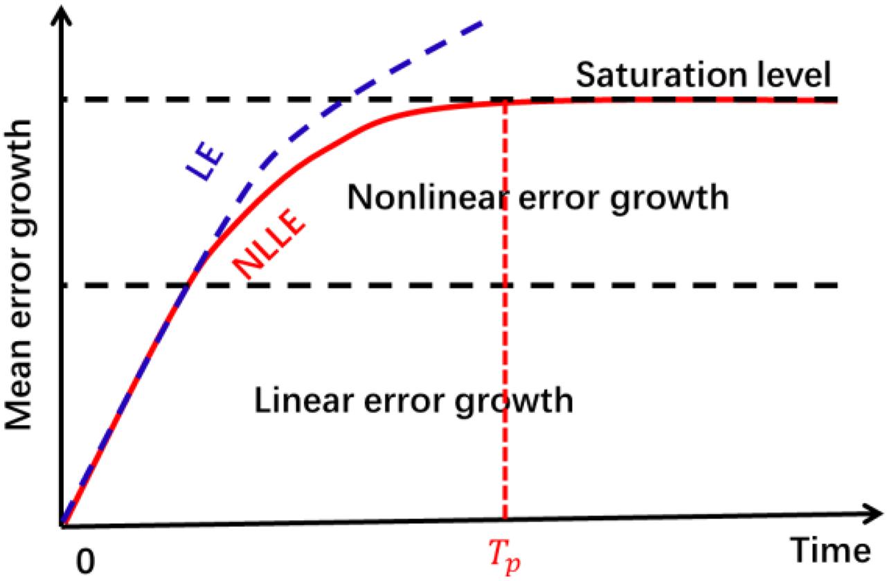
Figure 1. Schematic diagram of the mean error growth of a nonlinear dynamic system obtained by nonlinear local Lyapunov exponent (NLLE) (red) and traditional Lyapunov exponent (LE) (blue) approach. The mean error growth (y-axis) uses a logarithmic scale to amplify the differences between the linear and nonlinear error evolutions. Tp is the time that NLLE is reaching saturation status, which also stands for the predictability limit of NLLE (adopted and modified from Zhong et al., 2018).
The ensemble mean NLLE over the global attractor of the dynamical system is given by
where < > N denotes the ensemble mean of samples of sufficient sample size N(N→∞), and global attractor contains all the limit cases of the large-scale and long-term behavior of the system. The mean relative growth of the initial error (RGIE) can be obtained by
Based on the nonlinear error growth theory (Li and Ding, 2011), RGIE can be obtained as follows:
where denotes the convergence in probability, and the constant C is considered as the theoretical saturation value of when sample size N tends toward infinity. According to the definition, the predictability limit can be obtained to be Tp in Figure 1.
Estimation of NLLE From Eddy Tracks Dataset
Before computing NLLE using OME tracks, the analogous OMEs must be found out first. Li and Ding (2011) has developed an efficient algorithm based on local dynamical analogs (LDAs) to calculate the NLLE and its derivatives using observational data. For a chaotic system, the evolutions of two states are sure to be analogous over a short time interval if they are analogous at the initial stage (Lorenz, 1969; Wolf et al., 1985). The LDAs algorithm aims to seek analogous initial states and evolution patterns from the time series. Zhong et al. (2018) obtained the analogous TC tracks using LDAs. The analogous TC tracks are determined by the initial distance, evolutionary distance, seasonality, and initial intensity. Then, the predictability limit of TC tracks is measured by the divergence of the evolutionary tracks of two initially analogous OMEs.
Following Zhong et al. (2018), the determination of two analogous OME tracks is based on four factors: (a) initial distance d0 = d(t0), which is the distance between reference OME and analogous OME at the initial state (Figure 2); (b) the evolutionary distance de, which can be obtained by
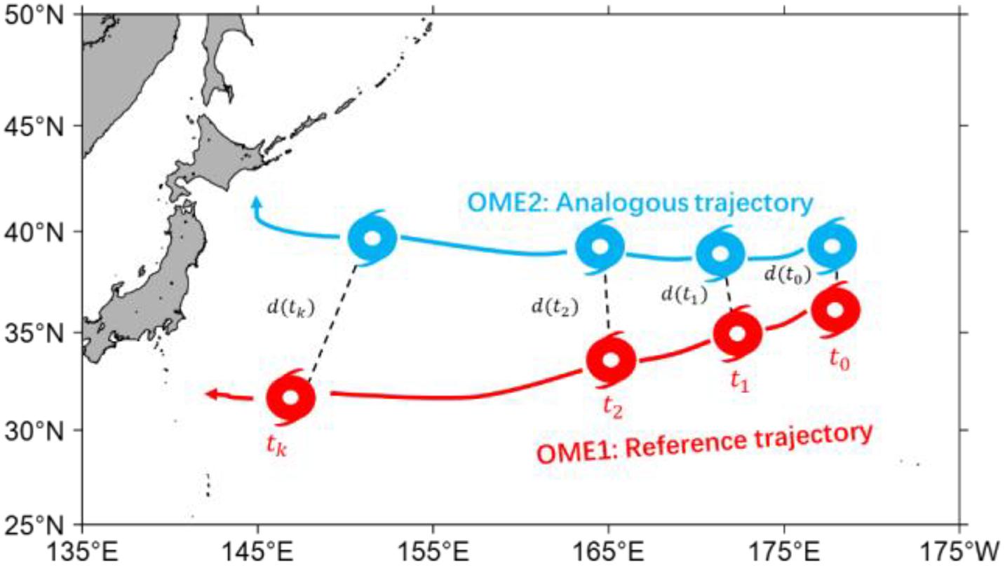
Figure 2. The schematic diagram of the procedure to calculate the nonlinear local Lyapunov exponent (NLLE) from the observational eddy track data. The trajectory of an analogous oceanic mesoscale eddy (OME) of the reference OME is denoted as the analogous trajectory. The absolute distance error’s growth rate between the reference OME and analogous OME at each time step (tk,k = 0,1,2,3,…) is used to estimate the NLLE.
where de is the mean distance between two analogous OMEs over the initial stage (from t1 to tK) after OMEs have formed; (c) the polarity of OMEs, which have been classified into cyclonic eddies (CEs) and anticyclonic eddies (AEs); (d) the intensity of OMEs, which is defined as the maximum of sea surface height anomaly. A minimal value of initial distance (d0) ensure that the genesis location of two independent OMEs is exceptionally close, and the small value of de ensure that the moving trajectories of two OMEs are consistent. Because the different polarity of OMEs have different physical characters and different spatial distribution (particular in the study region, Ji et al., 2018), it is necessary to seek analogous OMEs based on resembling polarity. However, no polarity preferences were found in the predictability limit of OME tracks in the following study. The conditions above are likely to exclude the nonanalogous OMEs as much as possible, thereby finding a truly local analog of the reference OME.
In the LDAs algorithm, the sum of d0 and de (dt) is used to determine the analog of two OMEs,
If dt is sufficiently small, the two OMEs is analogous at the initial time. The nearest neighbor of the reference OME can be chosen if dt is the minimum.
For every reference OME, we could identify its analogous OMEs if the total distance dt is small enough (Figure 2). The growth rate of the initial distance (error) at every time step, tk(k = 0,1,2,3,…), is denoted as follows:
The above steps are repeated for each analogous OME pair. From Equations (2), (3), and (4), we can obtain the approximation of the mean RGIE as follows:
Sensitivity Test of the Distance, the Time Steps, and the Sample Size
There are three primary parameters in the NLLE method above: the metrics of distance dt, the time steps of K for de, and the sample size. Before analyzing the results, these parameters’ sensitivity to the predictability limit has been scrutinized at first. Figure 3 shows the estimated predictability limit of OME tracks as a function of the dt, K, and the sample size.
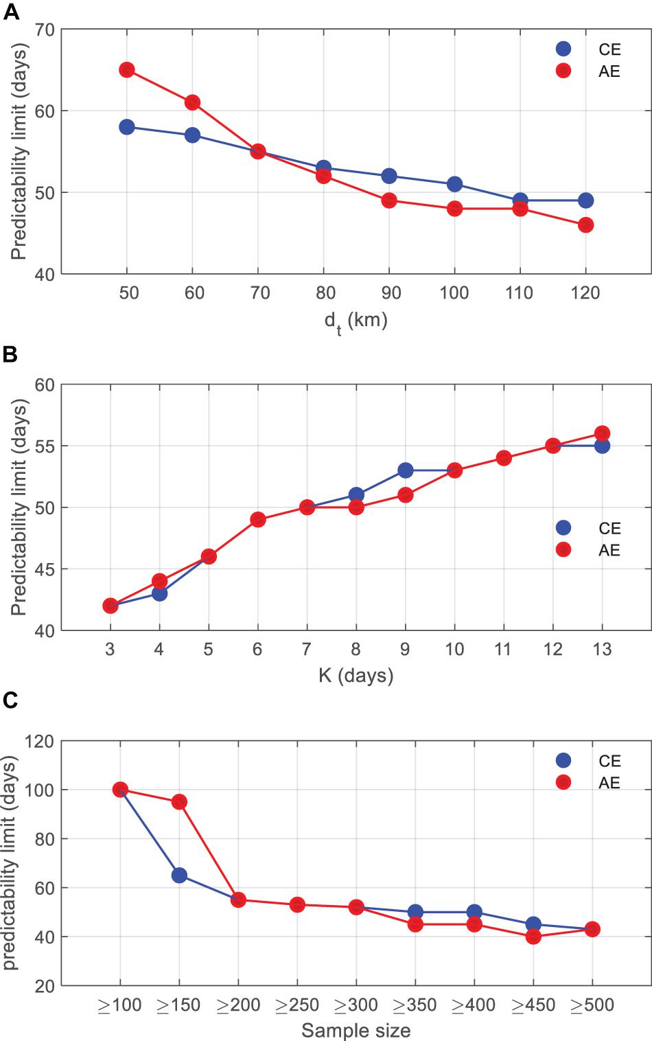
Figure 3. The sensitive tests of predictability limits of the oceanic mesoscale eddy (OME) tracks as a function of (A) dt (units: km), (B) K (units: days), and (C) the minimum sample size. The blue points are for CE, and red points are for AE.
A sufficiently large number of samples are required when applying the NLLE to estimate the predictability limit (Liu et al., 2016). However, the number of observational OMEs is finite. The OMEs track datasets are limited by the satellite observation period, which is only about 20–25 years. To obtain sufficient samples, one reference OME generally corresponds to multianalogous OMEs within limits of dt, which forms multianalogous pairs—on the other hand, increasing the criterion of dt also may find more analogous OMEs.
In Figure 3A, the predictability limit decreases with dt increasing from 50 to 110 km for every 10 km, which can be explained by Equation (1). The increases in dt means the increase in the initial error. As the initial error increasing, the NLLE value becomes smaller, and then, the predictability limit decreases. Here, we refer to the mean radius of the OMEs in the KE region (about 80 km) as the dt value. In this situation, the number of the analogous pairs we found reaches 2,791, which is a sufficient sampling based on the following results. Note that all the error herein is the distance of the center point between two independent OMEs.
According to the NLLE theory, two states are analogous at the initial time if their evolutions in phase space are analogous over a short time. The number of time steps, K, can help us exclude local nonanalogous states as much as possible. Figure 3B shows a gradual increase in predictability limit with the increasing value of K. We take no more than 6% of the average lifetime of the OMEs in the KE region as the value of K. A large K value weakens the error growth rate in the initial stage. Here, the initial time interval is 10 days.
The sample size is also a key parameter. The minimum sample size for computing the mean value of RGIE at a time tk is examined in Figure 3C. The predictability limit’s value becomes stable between 200 and 500, increasing 50 for every step, which means more than 200 samples must be used to get a stable value of the predictability limit. Here, we set the sample threshold as 300.
Results
The Properties of OMEs
Before estimating the predictability limit of OME tracks, we first examine the properties of OMEs in the KE region. According to Table 1, the differences between AEs and CEs in numbers, area–mean lifetime, amplitude, and radius are not significant. However, we found a large contrast for the CEs and AEs in the geostrophic distributions between northern and southern and between the eastern and western parts of the KE region. Previous studies have already pointed out that eddies’ lifetime longer than 50 weeks and shorter than 20 weeks are attributed to two different generation mechanisms (Ji et al., 2018).
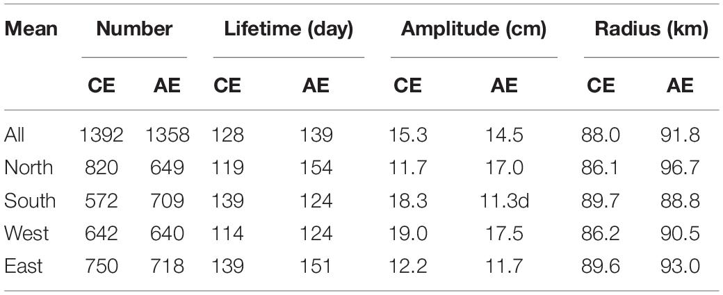
Table 1. The mean properties of the cyclonic eddies (CEs) and anticyclonic eddies (AEs) in the Kuroshio Extension (KE) region and its four subregions, namely, north (35°N–40°N, 143°E–175°W), south (30°N–35°N, 143°E–175°W), west (30°N–40°N, 143°E–160°E), and east (30°N–40°N, 160°E–175°W) during the period of 1993–2015.
Figure 4 shows the spatial distribution of the mean properties of OMEs in the central KE region for CEs (left panel) and AEs (right panel) in 2° × 2° grids, together with zonal and meridional mean curves. There is a smaller number of OMEs around the jet stream, around 30°N. Much more AEs tend to occur in the northern part of the region. The long-lived CEs and AEs locate on either side of the southern and northern areas of KE, CEs in the south part, and AEs in the north region. Similarly, the large amplitude values for CEs and AEs are also in the southern and northern regions. The mean radii of OMEs are relatively larger around the central axis of KE near 35°N.
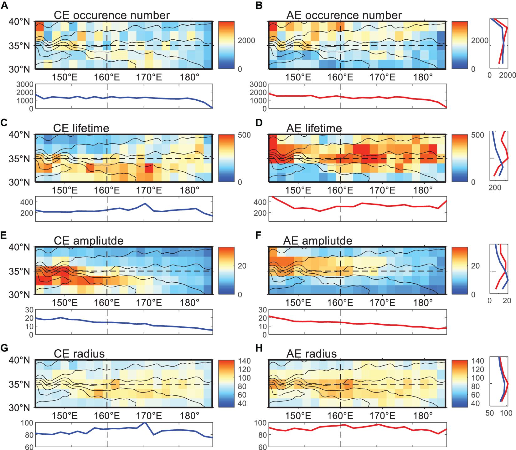
Figure 4. The means properties of the oceanic mesoscale eddies (OMEs) from Chelton in 2°× 2° grids for cyclonic eddies (CEs) (left panel) and anticyclonic eddied (AEs) (right panel). Panels (A,C,E,G) are the occurrence number, lifetime (unit: days), amplitude (unit: cm), and radius (unit: km) for CEs, respectively. Panels (B,D,F,H) are the same as panels (A,C,E,G) but for AEs. The black contours show the mean absolute dynamic topography from AVISO (MADT, unit: cm) during 1993–2015. The two dashed lines at 35°N and 160°E divide the area into four subregions. The right and bottom sides of each figure are the zonal and meridional mean results. Blue and the red color represents CEs and AEs.
Additionally, the OMEs properties are also different between the western and the eastern regions in the KE. The mean lifetime of OMEs in the east of KE is 25 days larger than that in the western part, and the radius shows the same trend (Table 1 and Figures 4C,D). Conversely, the mean amplitude of OMEs is larger in the west of KE, with 18 cm in the west and 12 cm in the east (Table 1 and Figures 4E,F).
We also investigated the characteristic of OME tracks for AEs and CEs in Figure 5. We found that more than 74% (2028) OMEs propagated westward, and only 26% (722) OMEs had a net eastward displacement. The ratio is like the values of Chelton et al. (2011) for the global domain, about 75 and 25%. The eastern propagation of OMEs is primarily caused by the strong eastward currents in this area (Chelton et al., 2011). To better see the tracks, we divided OMEs into three groups based on lifetime: <70 days, 70–182 days, and more than 182 days are shown in Figures 5A–F. The criterion is according to both the average lifetime and Chelton et al. (2011). The average lifetime is about 140 days in this region, and we set half of the average lifetime as the short-lived criterion. Chelton et al. (2011) used 182 days (26 weeks) as a criterion to analyze relative long-lived eddy trajectories. It is also long enough to represent the long-lived eddies in the KE region. The number of each polarity is labeled on the top of each panel. One notable characteristic is that the proportion of the eastward OMEs is much less in the long-lived OMEs. Another feature is that eastward CEs and AEs tend to occur in the north and south of KE. This phenomenon is evident in Figures 5B,D.
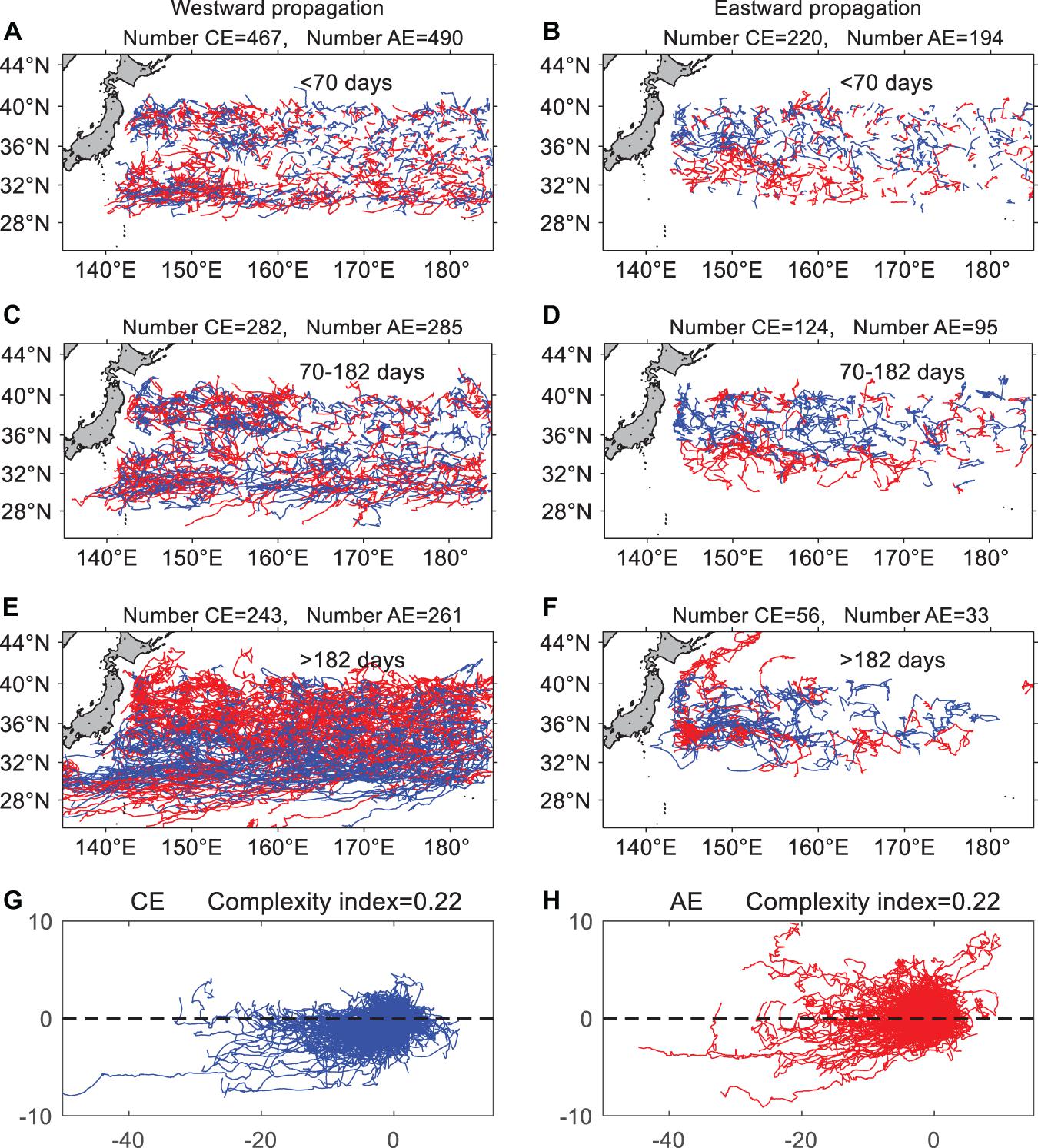
Figure 5. The oceanic mesoscale eddy (OME) trajectories with lifetimes shorter than 70 days for (A) westward OMEs and (B) eastward OMEs. Panels (C–F) are the same but for 70–182 days and more than 182 days. Panels (G,H) are normalized trajectories of OME tracks for all cyclonic eddies (CEs) (blue) and anticyclonic eddies (AEs) (red), respectively.
To measure the complexation of OME tracks, we define an eddy complexity index (CI) of OME trajectory as follow:
where D is the distance from the initial position to the termination position, and L represents the eddy trajectory’s distance during the part of or entire lifespan. CI is a positive number between 0 and 1. The more complex of the trajectory corresponds to the smaller of the CI. Figures 5G,H are normalized trajectories of OME tracks for all CEs (blue) and AEs (red). We found that CEs and AEs tend to have poleward and equatorward meridional deflections, respectively. This is consistent with the characteristic of eddy propagations revealed by other studies (e.g., Cheng et al., 2014). CEs and AEs have similar values of CI, 0.22. The eddy trajectories are usually about five times longer than the distance between the generation and termination position in this region. This also indicates that the predictability of CEs and AEs trajectories may have no significant difference in the whole KE region.
We also investigated the characteristic of the analogous OMEs only. The number of OMEs, which has found analogs, is 1593, accounting for 58%. The properties of analogous OMEs show that the spatial distribution of the analogous OMEs shares a similar pattern (Supplementary Figure 1), and the probability density function is identical (Supplementary Figure 2). Therefore, selecting analogous OMEs could represent the total samples in the KE region to estimate the predictability limit.
Mean Predictability Limit of the OME Tracks in the KE Region and Its Subregions
Figure 6 shows the CE and AE tracks’ mean error growth for the entire KE region from three datasets. Here, the mean error growth represents the RGIE, which is defined as the ratio of the real-time track error at the time of evolution to the initial distance. Based on the NLLE approach and the LDAs algorithm, the mean error growth of OME tracks can be obtained through Equation (8) using three eddy tracks datasets. The mean error of the OME tracks grow quickly at the initial stage, then enters a nonlinear growth phase. After 60 days, the error growth rate is almost zero, so the estimated saturation value is defined by the average of the relative error growth after the 60th day.
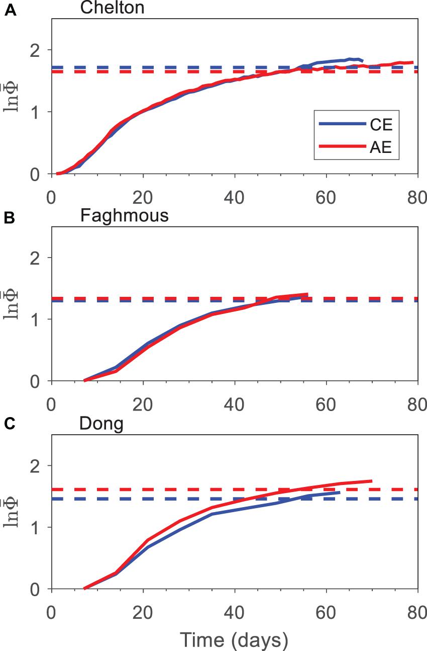
Figure 6. The mean error growth of all oceanic mesoscale eddy (OME) tracks in the Kuroshio Extension (KE) region obtained datasets of (A) Chelton, (B) Faghmous, and (C) Dong. The blue curves are for cyclonic eddies (CEs), and the red ones are for anticyclonic eddies (AEs). The dashed line represents the 95% level of the saturation value obtained by the mean value after the 60th day.
To reduce the effects of sampling fluctuations, we define the predictability limit as the time at which the mean error growth reaches 95% of saturation value following previous studies (Ding and Li, 2009; Li and Ding, 2013; Ding et al., 2016; Zhong et al., 2018). According to the saturation error, we determine that the predictability limit of OME tracks is 53 for CEs and 52 for AEs from Chelton datasets (Figure 6A). It should be noted that the saturation level mainly depends on the dynamical characteristics of the nonlinear system itself, and error depends on the analogous OMEs. Hence, it is, to some extent, a relatively objective criterion to quantitatively determine the predictability limit.
To estimate the uncertainties of the predictability limit due to datasets, we further calculated the values from both Faghmous and Dong (Figures 6B,C). The predictability limits of OME tracks obtained from these two datasets are primary in agreement with the results shown in Figure 6A, with the predictability values of 51/48 days for Faghmous and 53/53 days for Dong, <5% of Chelton’s values. This also indicates that the results seem not dependent much on the datasets or the methods to derive the eddy tracks. Hereafter, we mainly use the Chelton to discuss the predictability limit of the OME tracks.
We compute the spatial distribution of the OME tracks’ predictability limit obtained from Chelton (Figure 7). To calculate the spatial distribution, we first quantitatively estimated the predictability limit of the individual OME track. Then, the individual predictability limit was then averaged on 5° × 5°grids based on the generation locations. The predictability limit in the KE region (black box of Figure 7) ranges from 36 to 67 days and primarily affects by the genesis location of CEs and AEs. The predictability limit of the CE (AE) tracks in the southern (northern) part (20°N–35°N) is more significant than those in the northern (southern) part (35°N–40°N). These patterns are similar to the spatial distribution of number, polarity, lifetime, amplitude, and radius (Figure 4). Therefore, we speculate that the predictability limit might be related to eddies properties.
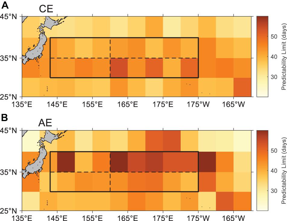
Figure 7. Spatial distribution of the area means predictability limit (days) of (A) cyclonic eddy (CE) and (B) anticyclonic eddy (AE) tracks in 5° × 5° grid boxes.
We further divided the entire region into four subregions: south (30°N–35°N, 143°E–175°W), north (35°N–40°N, 143°E–175°W), west (30°N–40°N, 143°E–160°E), and east (30°N–40°N, 160°E–175°W), as the black box shown in Figure 7. The mean error growth of the OME tracks in the four subregions is shown in Figure 8. The mean errors grow more rapidly and reach a saturation state faster in the western region than in the eastern region (Figures 8A,B). The CE and AE tracks’ overall predictability limit in the east region of KE is 65 and 60 days, which are approximately 2 weeks longer than that in the west, 52 and 40 days. Interestingly, CE tracks’ mean error increases more quickly and rapidly reaches a saturation level than that of AE tracks in the northern region, with the predictability limits of 54 and 66 days for CEs and AEs, respectively (Figure 8C). However, the situation is opposite in the southern region; CE tracks have a larger predictability limit (56 days) than that of AE tracks (42 days) (Figure 8D).
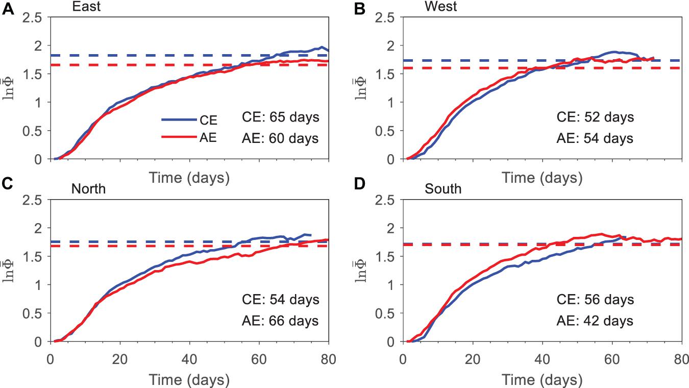
Figure 8. The same as Figure 6, but for the mean error growth of the oceanic mesoscale eddy (OME) tracks in the (A) eastern, (B) western, (C) northern, and (D) southern parts of the Kuroshio Extension (KE) region for Chelton. The blue curves are for cyclonic eddies (CEs), and the red ones are for anticyclonic eddies (AEs). The dashed line represents the 95% level of the saturation value obtained by the mean value after the 60th day.
According to the analysis above, there is a significant spatial pattern in the OME tracks’ predictability limit. To understand it, we show the mean trajectories of all the analogous OMEs in four subregions in Figure 9 and compute the CI of mean trajectories for the first 60 days and the whole period. We can find that the OMEs with smooth trajectories or large CI values tend to have longer predictability limits. It is evident that trajectories for both CEs and AEs in the eastern region are much smoother than those in the western region (Figures 9A,B). The CIs in the eastern region (0.82 for CEs and 0.93 for AEs) are also larger than those in the western region (0.61 for CEs and 0.86 for AEs) during the initial stage, even in the whole period. This can explain the longer predictability limit in the eastern part. The complexity of the western region’s trajectories might relate to the location close to the boundary or the relatively stronger background currents in this region. The CI also can explain the contrast between the southern and northern regions (Figures 9C,D). The tracks of CEs (AEs) in the northern (southern) part of the KE region have a shorter predictability limit and lower CI value than that of the southern region.
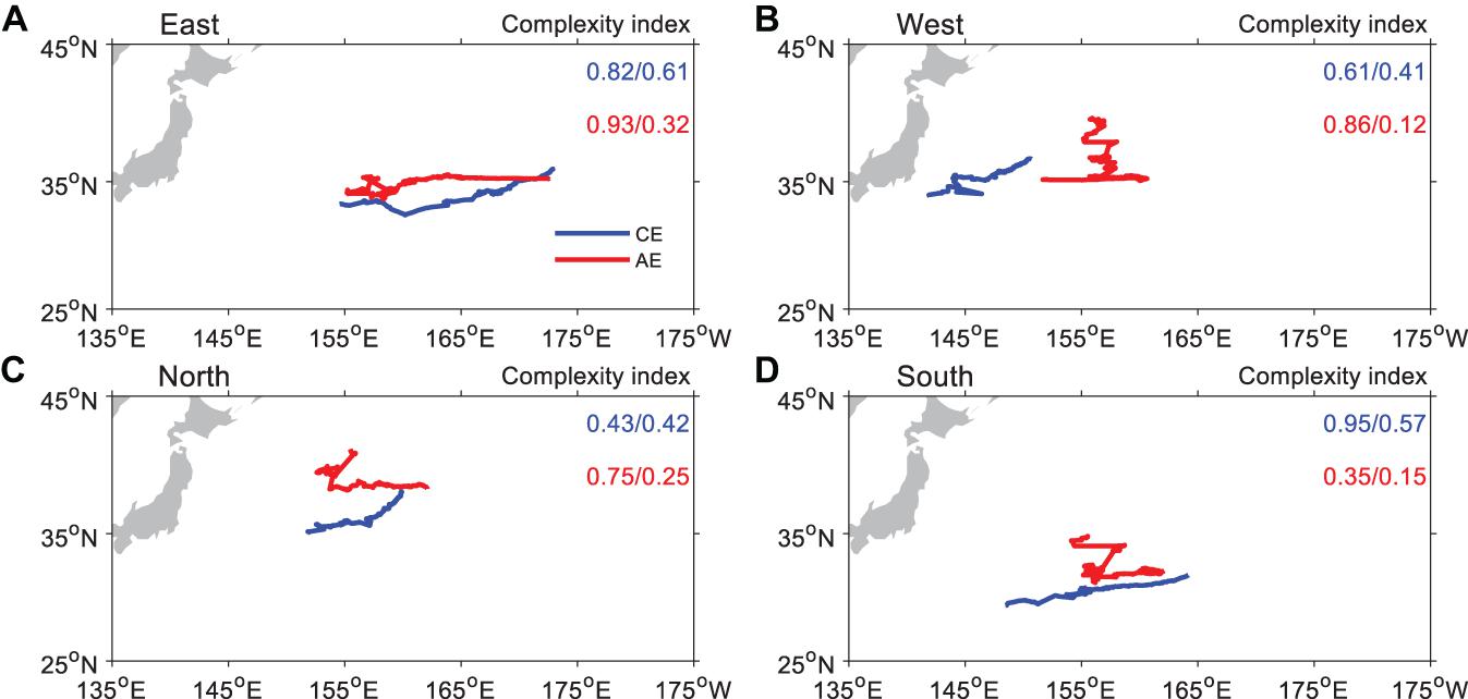
Figure 9. Mean tracks of the oceanic mesoscale eddies (OMEs) in the (A) East, (B) West, (C) North, and (D) South subregions. The blue curves are for cyclonic eddies (CEs), and the red ones are for anticyclonic eddies (AEs). The value of the Complexity Index (CI) of each mean trajectory is also shown in each figure. Before the slashes, the values are CIs for the first 60 days, while the whole lifetime after the slashes. The blue curves are for CEs, and the red ones are for AEs.
Predictability Limits for Different Lifetimes, Amplitudes, and Radii
The above section shows that the predictability limit of OME tracks vary in space. The predictability limit’s spatial distribution shares some common features with OME properties’ spatial distribution. The previous study of Early et al. (2011) suggested that the zonal propagating speeds of OMEs are related to their amplitude and size using a reduced gravity model, which indicated that the trajectory or the predictability limit of the trajectory of OMEs might vary with eddy properties. Therefore, it is necessary to consider the connection between properties and the predictability limit of OME tracks.
Figure 10 shows the predictability limits for different lifetimes, amplitudes, and radii, while the mean error growths are shown in Supplementary Figure 3 in the Supplementary Material. We classified a lifetime into two groups: short lived (<20 weeks) and long lived (>20 weeks). The classification criterion, 20 weeks, is based on the different OMEs generation mechanism, according to Ji et al. (2018). They found that the OMEs induced by flow shear are small and have a short time scale, while the OMEs generated by the development of meanders in the KE path are strong and have the longest lifetime. The analogous OME pairs for both short and long lifetimes are 1,560 and 237, respectively. This result indicates that the long-lived OMEs tend to have a longer predictability limit. According to the 95% saturation level, the predictability limit of short- and long-lived CE (AE) tracks is 57 (51) days and 110 (120) days (Figure 10A), respectively.
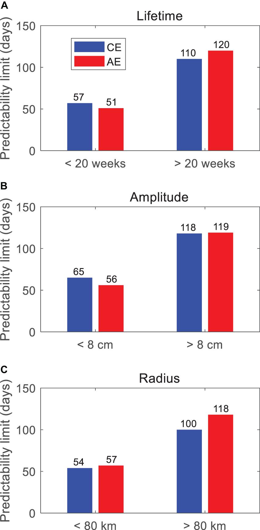
Figure 10. The predictability limits of oceanic mesoscale eddy (OME) tracks classified by different eddy properties, including (A) lifetime, (B) amplitude, and (C) radius. All the values are obtained by the 95% level of the saturation value received by the mean value of all OME tracks’ error growth after the 60th day. The blue bars are for CEs, and the red ones are for AEs (unit: days).
All OMEs are also classified into two groups according to the amplitude, namely, small amplitude (<8 cm) and large amplitude (>8 cm) (Figure 10B), and the radius, namely, small scale (<80 km) and large scale (>80 km) (Figure 10C). The amplitude and radius of OME often change throughout life; thus, the classification is based on the mean value during the entire lifespan. The results also clearly showed that the strong and large-size OMEs have the highest predictability limit. The predictability limit values for strong or large eddies are almost twice as those for weak or small ones.
We further investigated different categories’ mean trajectories to understand the relationship between eddy properties and their predictability of tracks (Figure 11). The start points are the averaged location for each type, which is consistent with the spatial distribution in Figure 4, the long life (short life), weak (strong), and small (large) eddies occurring in the eastern (western) part of the region. In general, the eddies have a longer life; the larger amplitude and the bigger size tend to have longer predictability limit. The longer and smoother trajectories for both CEs and AEs could explain for the larger predictability limit. However, the metrics to measure the complexation of eddy trajectories, CI, only works for CEs, not for AEs, particularly during the initial period (first 60 days). We find that the CI value is still not perfect for describing the complexity of the OME tracks. However, we can still observe that the trajectory’s movement characteristics are related to the predictability limit through observation.
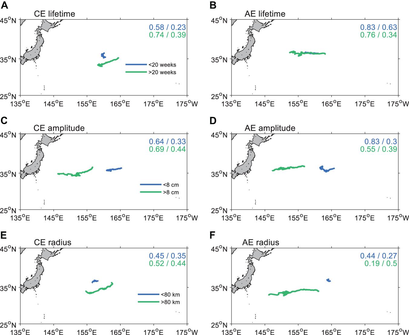
Figure 11. The mean trajectories of all cyclonic eddies (CEs) and anticyclonic eddies (AEs) for different (A,B) lifetime, (C,D) amplitude, and (E,F) radius. The value of the Complexity Index (CI) of each mean trajectory is also shown in each figure. Before the slashes, the values are CIs for the first 60 days while the whole lifetime after the slashes.
As shown in Figure 4, the longer lifetime OMEs usually occurred in the eastern region. This is also consistent with the geostrophic distribution of the predictability limit shown in the previous section (Figures 7, 8). The OME tracks in the east part of the target region tend to have a longer predictability limit. However, the stronger eddies also have a longer predictability limit, which seems contradicted with the spatial distribution. The stronger eddies usually occur in the western part (Figures 4E,F). This indicates that the relationship between the eddy properties and the predictability limit is complicated, and factors other than eddy properties may affect the limit.
External Environment of the KE Region
Besides the eddy properties, the OME trajectories are also affected by the ocean and atmosphere’s large-scale motions. Figure 12A shows the mean sea surface height (SSH, shaded) and the geostrophic current (vectors) from Mercator Ocean reanalysis data over 14 years, which is available on the Copernicus Marine Environment Monitoring Service (CMEMS) website.2 The red curve is the approximate location of the central axis of the Kuroshio current. We can find that the larger meridional gradient of SSH, stronger surface currents, and the larger meander of the Kuroshio current all appear in the western region. These will lead the OMEs much easier to change their trajectories and become unpredictable. The magnitude of surface wind in the KE region (Figure 12B) is more than 7 m/s. Still, it is relatively homogeneous in our study domain, indicating that the mean surface wind may not affect the movement of OMEs very much.
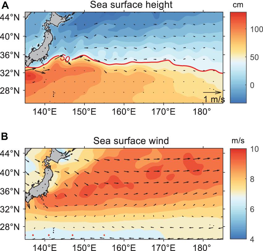
Figure 12. The spatial distribution of (A) annual mean sea surface height (contour, units: cm) geostrophic current (vectors) from Mercator Ocean analysis data from 1993 to 2006 and (B) annual mean sea surface wind from National Oceanic and Atmospheric Administration (NOAA) from 1999 to 2009 (units: m/s).
The mean currents in the KE region could be one of the significant impacts on the OME tracks. To further illustrate the unstable statement of KE currents, Figure 13 shows the standard deviation of monthly mean SSH and velocities in both zonal and meridional directions from 1993 to 2006. The whole KE region has a large amplitude for SSH and speeds, with the largest values occurring in the western part, more than 0.4 m for SSH and 0.4 m/s for speeds. This may suggest that surface currents are more unstable in the west region and may lead to shorter predictability limits.
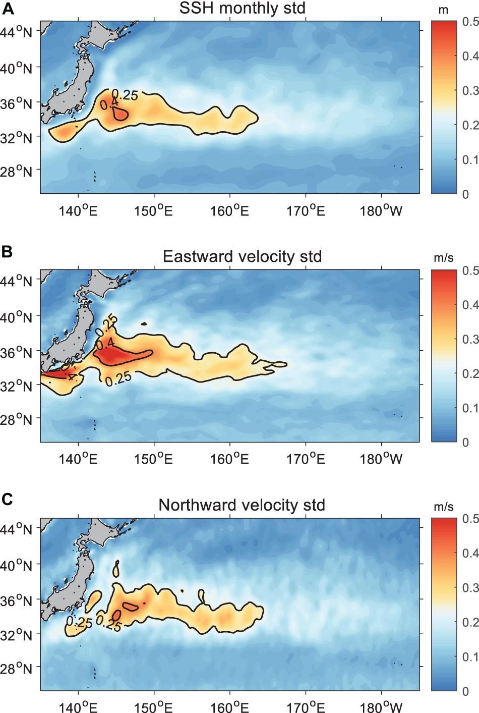
Figure 13. The standard deviation of the monthly mean (A) surface sea level (units: m), (B) eastward, and (C) northward geostrophic velocity from Mercator Ocean analysis data during the period of 1993–2006 (units: m/s).
Conclusion and Discussion
Conclusion
Based on the NLLE approach and LDAs algorithms, we estimate the predictability limit in the whole KE region quantitively using three eddy track datasets. The results show that the predictability limits of CEs and AEs are 53 and 52 days in KE and vary in the four subregions ranging from 42 to 66 days. The predictability limit of OME tracks is higher in the eastern region (about 62.5 days) than that in the western region (about 46 days), implying that daily OME tracks’ prediction is more challenging in the nearshore region than in the opened sea area. Additionally, the CEs (AEs) predictability limit is relatively high in the southern (northern) region.
The predictability limit of OME also tracks closely related to lifetime, amplitude, and radius. The long-lived, large-amplitude, and large-size OMEs tend to be more predictable with more than 100 days, whereas short-lived, small-amplitude, and small-size OMEs tend to be less predictable with the value of about 60 days.
We have proposed a metrics called the Complexity Index (CI) to examine the OME tracks’ smoothness to understand the predictability limit. It turns out that the OMEs with smooth trajectories or large CI tend to have longer predictability limits in most cases. We examined the differences in the function of life duration and CI among four subregions and found that a shorter predictability limit has a much rapid decrease for CI values. However, the CI does not work well for AEs in the different classification of OME properties.
Besides the properties of OME, the external oceanic and atmospheric environment also can affect the predictability of OME tracks. The Kuroshio axis is stronger and has larger variability in the region close to the western boundary, which will shorten the limit in this area. The external effects may explain why the west subregion has strong eddies but a shorter predictability limit. We also found that the surface wind may not contribute to the instability much.
Based on our analysis, three kinds of factors may affect the predictability limit of eddy tracks. The first factor is the boundary, which would change the eddy trajectories when eddy gets close to the boundary. The second factor is the characters of eddies, such as the amplitude, the radius, and the lifetime. The stronger and larger eddies would not be affected by the external factors and will be more predictable. The third is the background currents or winds. The former will interact with the eddies, and the latter will directly force the eddies and change their path.
Discussion
In addition to the eddy features like the amplitude, the radius, and the lifetime, we have also investigated the predictability limit of eddy tracks based on different nonlinear parameters before. However, the result is not shown in the paper. The results show that CE/AE with a higher U/c tends to have a larger predictability limit. The predictability limit of weak-nonlinear (U/c < 5) and strong-nonlinear (U/c > 7) CE tracks are 29 and 39 days, respectively, but 33 and 90 days for AE. Therefore, the stronger nonlinear eddies generally have a longer predictability limit.
The present study shows that the predictability limit of OME tracks is not dependent on datasets, although the trajectories in Figure 5 of Meng et al. (2020) look totally different. We found that the average trajectories of these three datasets (Figure 5 in Meng et al., 2020) almost overlap in the initial stage and begin to diverge after about 200 days (or longitude less than −3°). The mean predictability limit of OME tracks is only about 50 days, and therefore, the predictability limit mainly depends on the initial stage of trajectories.
The predicted time scales in the previous studies are approximately 30 days (Li et al., 2019; Xu et al., 2019; Wang et al., 2020), while the predictability limits of the OME tracks computed in the present study are more than 50 days. It seems about 1.5–2 times greater than that in previous studies. We think that two reasons perhaps cause the longer predictability limit in the present studies. First is the study region being different. This leads to the features of eddies, and the environment is also different. Here, we study the KE region, while Xu et al. (2019) and Li et al. (2019) investigated the South China Sea, and Wang et al. (2020) focused on the whole global. Second, the previous studies did not focus on the upper limit of predictability as to the present study. In these studies, the eddy features may be predicted before approximately 1 month. However, they did not try to explore the upper limit. Additionally, there are only two cases in Xu et al. (2019), which cannot be compared with the present study.
Although we discuss the relationship between eddy properties and predictability and external environment, the effect of eddy–eddy interactions are excluded. A recent paper by Ni et al. (2020) pointed out that the interaction between these OMEs would potentially affect trajectories and lead to moving randomly in any direction at any latitude. An earlier study also has indicated that eddy–eddy interactions on the eddy propagation help induce the eddy trajectory curve or loop (Early et al., 2011). These studies suggest that the eddy–eddy interaction might affect the predictability limit of eddy tracks to some extent. The effects of the eddy–eddy interaction on the results of the present study should be investigated further.
This study helps us understand the predictability of OMEs. These results cannot directly apply to the real operational forecast; however, the predictability limit can provide a baseline for forecasting in this region. In the future, model simulation analysis will be needed to explore more in-depth both the physical understanding and the impact of external factors on the predictability.
Data Availability Statement
The original contributions presented in the study are included in the article/Supplementary Material, further inquiries can be directed to the corresponding author/s.
Author Contributions
YM and HL conceived the study and preformed most of the analysis and writing. RD, PL, MD, and PW contributed data and other information, as well as assisting with writing and analysis. All authors contributed to the article and approved the submitted version.
Funding
This study was supported by the National Natural Science Foundation of China (Grants 41931183, 41976026, and 41931182), the National Key R&D Program for Developing Basic Sciences (2018YFA0605703), and the Strategic Priority Research Program of the Chinese Academy of Sciences (Grant no. XDB42010404). The authors, HL and PL, also acknowledge the technical support from the National Key Scientific and Technological Infrastructure project “Earth System Science Numerical Simulator Facility” (EarthLab).
Conflict of Interest
The authors declare that the research was conducted in the absence of any commercial or financial relationships that could be construed as a potential conflict of interest.
Acknowledgments
We are grateful for the mesoscale eddy datasets provided by Chelton et al. (2011); Faghmous et al. (2013), and Dong et al. (2011).
Supplementary Material
The Supplementary Material for this article can be found online at: https://www.frontiersin.org/articles/10.3389/fmars.2021.658125/full#supplementary-material
Footnotes
References
Chelton, D. B., Schlax, M. G., and Samelson, R. M. (2011). Global observations of nonlinear mesoscale eddies. Prog. Oceanogr. 91, 167–216. doi: 10.1016/j.pocean.2011.01.002
Chen, B., Li, J., and Ding, R. (2006). Nonlinear local Lyapunov exponent and atmospheric predictability research. Sci. China Ser. D 49, 1111–1120. doi: 10.1007/s11430-006-1111-0
Chen, Y. L. L., Chen, H. Y., Lin, I. I., Lee, M. A., and Chang, J. (2007). Effects of cold eddy on phytoplankton production and assemblages in luzon strait bordering the south china sea. J. Oceanogr. 63, 671–683. doi: 10.1007/s10872-007-0059-9
Cheng, Y., Ho, C., Zheng, Q., and Kuo, N. (2014). Statistical characteristics of mesoscale eddies in the north pacific derived from satellite altimetry. Remote Sens. 6, 5164–5183. doi: 10.3390/rs6065164
Ding, R., and Li, J. (2007). Nonlinear finite-time Lyapunov exponent and predictability. Phys. Lett. A 364, 396–400. doi: 10.1016/j.physleta.2006.11.094
Ding, R., and Li, J. (2009). Long-term trend and decadal variability of persistence of daily 500-mb geopotential height anomalies during boreal winter. Mon. Wea. Rev. 137, 3519–3534. doi: 10.1175/2009mwr2841.1
Ding, R., and Li, J. (2012). Relationships between the limit of predictability and initial error in the uncoupled and coupled Lorenz models. Adv. Atmos. Sci. 29, 1078–1088. doi: 10.1007/s00376-012-1207-8
Ding, R. Q., Li, J. P., Zheng, F., Feng, J., and Liu, D. Q. (2016). Estimating the limit of decadal-scale climate predictability using observational data. Climate Dyn. 46, 1563–1580. doi: 10.1007/s00382-015-2662-6
Dong, C., Nencioli, F., Liu, Y., and McWilliams, J. C. (2011). An automated approach to detect oceanic eddies from satellite remotely sensed sea surface temperature data. IEEE Geos. Rem. Sens. Let. 8, 1055–1059. doi: 10.1109/LGRS.2011.2155029
Early, J. J., Samelson, R. M., and Chelton, D. B. (2011). The evolution and propagation of quasigeostrophic ocean eddies. J. Phys. Oceanogra. 41, 1535–1555. doi: 10.1175/2011JPO4601.1
Faghmous, J. H., Le, M., Uluyol, M., Kumar, V., and Chatterjee, S. (2013). “A parameter-free spatio-temporal pattern mining model to catalog global ocean dynamics,” in Proceedings of the 2013 IEEE 13th International Conference on Data Mining, (Dallas, TX), 151–160.
Farneti, R., Delworth, T. L., Rosati, A. J., Griffies, S. M., and Zeng, F. (2010). The role of mesoscale eddies in the rectification of the Southern Ocean response to climate change. J. Phys. Ocean. 40, 1539–1557. doi: 10.1175/2010JPO4353.1
Ferrari, R., and Wunsch, C. (2009). Ocean circulation kinetic energy: reservoirs, sources, and sinks. Ann. Rev. Flui Mec. 41, 253–282. doi: 10.1146/annurev.fluid.40.111406.102139
Hallberg, R., and Gnanadesikan, A. (2006). The role of eddies in determining the structure and response of the wind-driven Southern Hemisphere overturning: Results from the Modeling Eddies in the Southern Ocean (MESO) project. J. phys. Ocean. 36, 2232–2252. doi: 10.1175/JPO2980.1
Hurlburt, H. E., Chassignet, E. P., Cummings, J. A., Kara, A. B., and Metzger, E. J. (2009). Eddy-resolving global ocean prediction. Geophys. Monograph. 177, 353–381. doi: 10.1029/177GM21
Ji, J., Dong, C., Zhang, B., Liu, Y., and Chen, D. (2018). Oceanic eddy characteristics and generation mechanisms in the kuroshio extension region. J. Geophys. Res. Oceans. 123, 8548–8567. doi: 10.1029/2018JC014196
Li, J., and Ding, R. (2011). Temporal-spatial distribution of atmospheric predictability limit by local dynamical analogs. Mon. Wea. Rev. 139, 3265–3283. doi: 10.1175/MWR-D-10-05020.1
Li, J., and Ding, R. (2013). Temporal-spatial distribution of the predictability limit of monthly sea surface temperature in the global oceans. Inter. J. Clim. 33, 1936–1947. doi: 10.1002/joc.3562
Li, J., Wang, G., Xue, H., and Wang, H. (2019). A simple predictive model for the eddy propagation trajectory in the northern south china sea. Ocean Sci. 15, 401–412. doi: 10.5194/os-15-401-2019
Liu, J., Li, W., Chen, L., Zuo, J., and Zhang, P. (2016). Estimation of the monthly precipitation predictability limit in China using the nonlinear local Lyapunov exponent. J. Meteo. Re. 30, 93–102. doi: 10.1007/s13351-015-5049-z
Lorenz, E. N. (1969). The predictability of a flow which processes many scales of mothion[J]. Tellus 21, 289–307. doi: 10.1111/j.2153-3490.1969.tb00444.x
Meng, Y., Liu, H., Lin, P., Ding, M., and Dong, C. (2020). Oceanic mesoscale eddy in the Kuroshio Extension: comparison of four datasets. Atm. Oce. Sci. Let. 14:100011. doi: 10.1016/j.aosl.2020.100011
Ni, Q., Zhai, X., Wang, G., and Marshall, D. P. (2020). Random movement of mesoscale eddies in the global ocean. J. Phys. Oceanogra. 50, 2341–2357. doi: 10.1175/JPO-D-19-0192.1
Pinardi, N., Bonazzi, A., Dobricic, S., Milliff, R. F., Wikle, C. K., and Berliner, L. M. (2011). Ocean ensemble forecasting. Part II: mediterranean forecast system response. Q. J. R. Meteorol. Soc. 137, 879–893.
Wang, X., Wang, H., Liu, D., and Wang, W. (2020). The prediction of oceanic mesoscale eddy properties and propagation trajectories based on machine learning. Water 12:2521. doi: 10.3390/w12092521
Wolf, A., Swift, J. B., Swinney, H. L., and Vastano, J. A. (1985). Determining Lyapunov exponents from a time series. Phys. D: Nonlinear Phenomena 16, 285–317. doi: 10.1016/0167-2789(85)90011-9
Xiu, P., and Chai, F. (2011). Modeled biogeochemical responses to mesoscale eddies in the South China Sea. J. Geophys. Res. Oceans 116:C10006. doi: 10.1029/2010jc006800
Xu, D., Zhuang, W., and Yan, Y. (2019). Could the two anticyclonic eddies during winter 2003/2004 be reproduced and predicted in the northern South China Sea? Oce. Sci. 15, 97–111. doi: 10.5194/os-15-97-2019
Zhang, Z., Wang, W., and Qiu, B. (2014). Oceanic mass transport by mesoscale eddies. Science 345, 322–324.
Keywords: mesoscale eddy, predictability limit, Kuroshio Extension, nonlinear local Lyapunov exponent (NLLE), eddy tracks
Citation: Meng Y, Liu H, Ding R, Lin P, Ding M and Wang P (2021) The Predictability Limit of Ocean Mesoscale Eddy Tracks in the Kuroshio Extension Region. Front. Mar. Sci. 8:658125. doi: 10.3389/fmars.2021.658125
Received: 25 January 2021; Accepted: 28 May 2021;
Published: 02 July 2021.
Edited by:
Zhiyu Liu, Xiamen University, ChinaReviewed by:
Adam Thomas Devlin, Jiangxi Normal University, ChinaZhengguang Zhang, Ocean University of China, China
Guihua Wang, Fudan University, China
Copyright © 2021 Meng, Liu, Ding, Lin, Ding and Wang. This is an open-access article distributed under the terms of the Creative Commons Attribution License (CC BY). The use, distribution or reproduction in other forums is permitted, provided the original author(s) and the copyright owner(s) are credited and that the original publication in this journal is cited, in accordance with accepted academic practice. No use, distribution or reproduction is permitted which does not comply with these terms.
*Correspondence: Hailong Liu, bGhsQGxhc2cuaWFwLmFjLmNu; Pengfei Lin, bGlucGZAbWFpbC5pYXAuYWMuY24=