Drivers of Spatial Distributions of Basking Shark (Cetorhinus maximus) in the Southwest Pacific

Finucci, Brittany; Duffy, Clinton A. J.; Brough, Tom; Francis, Malcolm P.; Milardi, Marco; Pinkerton, Matthew H.; Petersen, Grady; Stephenson, Fabrice

doi:10.3389/fmars.2021.665337

ORIGINAL RESEARCH article

Front. Mar. Sci., 26 April 2021

Sec. Marine Megafauna

Volume 8 - 2021 | https://doi.org/10.3389/fmars.2021.665337

Drivers of Spatial Distributions of Basking Shark (Cetorhinus maximus) in the Southwest Pacific

$\r\nBrittany Finucci*$ Brittany Finucci^1*

Clinton A. J. Duffy²

Tom Brough³

Malcolm P. Francis¹

Marco Milardi⁴

Matthew H. Pinkerton¹

Grady Petersen³

Fabrice Stephenson³

¹National Institute of Water and Atmospheric Research (NIWA), Wellington, New Zealand
²Department of Conservation, Auckland, New Zealand
³National Institute of Water and Atmospheric Research (NIWA), Hamilton, New Zealand
⁴Fisheries New Zealand - Tini a Tangaroa, Ministry for Primary Industries - Manatū Ahu Matua, Wellington, New Zealand

Basking sharks (Cetorhinus maximus) were widely reported throughout New Zealand waters. Once commonly observed, and sometimes in large numbers, basking sharks are now infrequently reported. Basking shark observations are known to be highly variable across years, and their distribution and occurrence have been shown to be influenced by environmental predictors such as thermal fronts, chl-a concentration, and the abundance of prey (zooplankton). Little is known of basking sharks in the South Pacific and more information on distribution, habitat use, and migratory patterns is required to better understand the species’ regional ecology. Here, we used bootstrapped Habitat Suitability Models [HSM, ensembled from Boosted Regression Tree (BRT) and Random Forest (RF) models] to determine the drivers of basking shark distribution, predict habitat suitability and estimated uncertainty in the South Pacific for the first time. High−resolution environmental (1 km² grid resolution) and biotic data, including inferred prey species, and all available basking shark records across New Zealand’s Exclusive Economic Zone (EEZ) were included in the ensemble HSMs. The most influential driver of modeled basking shark distribution was vertical flux of particulate organic matter at the seabed, which may indicate higher levels of primary production in the surface ocean and higher prey density in the mesopelagic zone and at the seafloor. The BRT and RF models had good predictive power (AUC and TSS > 0.7) and both models performed similarly with low variability in the model fit metrics. Areas of high basking shark habitat suitability included the east and west coasts of the South Island, Puysegur Ridge, and Auckland Island slope. The outputs produced here could be incorporated into future management framework for assessing threat and conservation needs (e.g., spatially explicit risk assessment) for this regionally protected species, as well as providing guidance for future research efforts (e.g., areas of interest for sampling).

Introduction

The basking shark (Cetorhinus maximus) is a planktivorous coastal-pelagic species widely distributed in the temperate and tropical waters of the Atlantic and Pacific Oceans, and fringes of the Indian Ocean (southern Australia, Indonesia, South Africa) (Rigby et al., 2019). It is the second largest fish in the world after the whale shark (Rhincodon typus), reaching an maximum size greater than 10 m total length (Weigmann, 2016). Basking sharks are known for their slow surface swimming behavior but may also spend months at mesopelagic depths, and may dive to at least 1,264 m depth (Gore et al., 2008; Skomal et al., 2009; Dewar et al., 2018). The species also engages in long distance migrations and has been recorded crossing the Atlantic Ocean both from east to west and from north to south (Skomal et al., 2009; Braun et al., 2018; Dewar et al., 2018; Johnston et al., 2019). Recent genetic analysis suggests high gene flow and weak genetic structuring across the Atlantic and Pacific Oceans (Lieber et al., 2020). Despite their large size, basking sharks remain elusive and data-poor in the Pacific Ocean; habitat use and movement patterns in the South Pacific, and more specifically around New Zealand, are poorly understood.

New Zealand was once a hotspot for basking sharks in the South Pacific Ocean. Historically, the species was common in New Zealand coastal and offshore waters between 39°S and 51°S. Most records were from south of Cook Strait in cold, nutrient-rich waters along the Subtropical Front (Francis and Duffy, 2002). Individuals and large schools were most commonly reported during the spring and summer months along the east coast of the South Island and off Snares-Auckland Islands (Francis, 2017). Aerial surveys for Hector’s dolphins (Cephalorhynchus hectori) conducted around Bank’s Peninsula (east coast of the South Island) reported large groups of over 100 individuals in the early 1990s (Francis and Duffy, 2002). Subsequent aerial surveys for basking sharks and Hector’s dolphins have not seen any basking sharks. Only a few individuals are now reported annually, primarily as fisheries bycatch (Francis, 2017). Beyond New Zealand, basking sharks have been very infrequently observed across the South Pacific Ocean (Yatsu, 1995; Hernández et al., 2010).

Basking sharks are susceptible to exploitation from fishing due to their naturally low population sizes, presumed slow growth rates, and low reproductive rates (Francis, 2017). The species was subject to targeted fishing throughout its range and while most targeted fisheries ceased in the 2000s, basking sharks are still taken as bycatch by a number of fishing gear types (e.g., trawl, trammel net, set net). Elsewhere they are threatened by interactions with recreational vessels and commercial shipping due to the species’ time spent at the surface (Austin et al., 2019; Rigby et al., 2019). Population recovery has been low or negligible up to two decades after fishing ceased (Fowler et al., 2005). In 2002, basking sharks were listed in Appendix II of the Convention on International Trade in Endangered Species of Wild Fauna and Flora (CITES, 2002), and in 2005, were listed on Appendices I and II in the Convention of Migratory Species (CMS). In 2019, basking shark was assessed as globally Endangered by the International Union for Conservation of Nature (IUCN) Red List of Threatened Species (Rigby et al., 2019).

Basking sharks have been protected in New Zealand waters since 2010. There are no specific management measures in place for basking sharks, apart from mandatory reporting of captures and the return of captured individuals to the sea. There are very few fisheries independent data available and estimates of basking shark bycatch likely underestimate the total New Zealand catches because they do not account for captures in unobserved set net fisheries and inshore trawl fisheries (Francis, 2017). Patterns in unstandardized catch-per-unit-effort (CPUE) imply basking sharks were captured in relatively large numbers in the late 1980s and early 1990s, with peak bycatch occurring between 1988 and 1991 (Francis, 2017). Following this period, observed bycatch rates declined substantially. Off the east coast of the South Island raw CPUE peaked in 1991 at 81.9 sharks per 1,000 tows then fell to zero reported captures from 2005–2016 (Francis, 2017). In recent years, the species has occasionally been taken as bycatch in trawl and set net fisheries, with trawl bycatch typically occurring near or beyond the edge of the continental shelf (Francis and Smith, 2010; Francis, 2017). It is unclear if the recent decline in basking shark records in New Zealand is a result of a change to fishing practices that are less likely to encounter basking sharks, changes in regional availability of sharks, a real decline in abundance or a combination of these (Francis, 2017).

Distributions of basking shark are known to be highly variable between years, with up to 20 years between sightings reported from some Northern Hemisphere locations (Dewar et al., 2018). Their distribution and occurrence appears to be strongly linked to zooplankton/prey abundance at smaller spatial scales, but the drivers of broad scale distribution patterns are largely unknown (Sims, 2008). In the Northern Hemisphere, environmental predictors such as sea surface temperature (SST), thermal fronts, chl-a concentration, and the abundance of zooplankton seem to influence their distribution (Cotton et al., 2005; Austin et al., 2019). However, without sufficient information on the species’ distribution, habitat use, and migratory patterns, it is difficult to determine the cause of variability in abundance and distribution.

Correlative models that predict the occurrence of species in relation to environmental variables (termed habitat suitability models or species distribution models) have become an important part of resource management and conservation biology. Such models are capable of filling knowledge gaps on spatial and temporal distributions and predicting areas of suitable habitat for widely distributed species (Elith et al., 2006; Weber et al., 2017). By relating species’ sightings to environmental predictor variables, the abundance or probability of taxa presence at a given location can be estimated along with a characterization of the environmental drivers of species distributions. These models are becoming increasingly popular for use on marine species spanning large geographic and bathymetric ranges and have been employed for a range of cetaceans (Stephenson et al., 2020b), seabirds (Cleasby et al., 2020), and cartilaginous fishes, including basking sharks in the Northeast Atlantic (Austin et al., 2019).

Here, we combine functionally relevant, high−resolution environmental data (1 km² grid resolution) with data on basking shark occurrences to predict basking shark habitat suitability across New Zealand’s Exclusive Economic Zone (EEZ). Unlike many habitat suitability models which include only environmental data and primary productivity, here we had the unique opportunity to also include high trophic level biotic data (zooplankton prey densities). The distribution of prey is often unavailable or overlooked, and at times, is a key predictor of species’ distributions (Dormann et al., 2018; Carroll et al., 2019). Understanding biotic interactions and their influence in driving species’ distributions is important for predicting into unsampled space because the trophic interactions that are at the core of species habitat use may be better captured (e.g., more accurate predictions due to climate change) (Araújo and Luoto, 2007). Regional differences in drivers of species’ distribution can also be present (Petatan-Ramirez et al., 2020). Thus, identifying factors that drive basking shark distribution across the New Zealand marine region is important for better understanding the species’ regional ecology and to direct and inform future research and spatially explicit conservation efforts for this protected species.

Materials and Methods

Study Area

The study area extends over 4.2 million km² of the South Pacific Ocean within the New Zealand EEZ (≈ 25–57°S; 162°E–172°W; Figure 1). New Zealand’s EEZ contains highly productive zones of mixing between warm, higher salinity, nutrient poor, northern waters, and cold, lower salinity, nutrient rich, southern waters. These productive zones support high biological diversity and a variety of customary, recreational, and commercial fisheries (Bradford-Grieve et al., 2006; Leathwick et al., 2006; Stephenson et al., 2018, 2020a). The New Zealand continental shelf environment is influenced by a combination of climatic features that produce a range of nearshore conditions, upwelling, tidal mixing, and upper-ocean mixing. Surface and thermocline waters of different origin are separated by three major fronts, the Subtropical Front, the Subantarctic Front, and the Polar Front, while the flow of bottom water is predominately carried by the Deep Western Boundary Current (Chiswell et al., 2015). New Zealand bathymetry is equally as complex, reaching abyssal depths beyond 10,000 m in the Kermadec Trench and includes over 800 distinct sea features (Rowden et al., 2005; Linley et al., 2017).

FIGURE 1

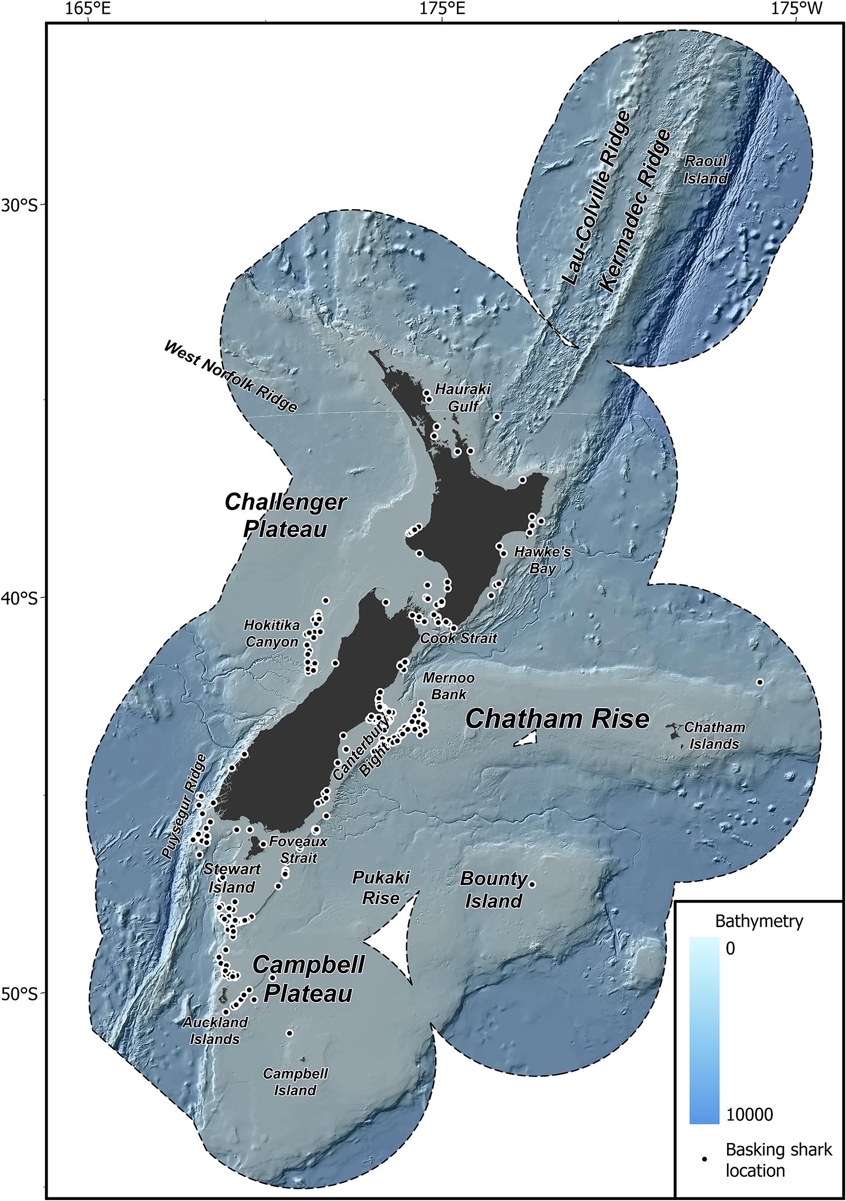
Figure 1. Map of the study region. New Zealand Exclusive Economic Zone (EEZ, black dashed line), bathymetry, and feature names used throughout the text modified from Stephenson et al. (2020a), and the location of basking shark records used in this study (black dots).

Species Records

Basking shark records (n = 401) were collated from various sources including records from observed and self-reported captures in commercial fisheries, public sightings, media reports, museum records, fishery surveys, aerial surveys and beach cast specimens. Records variously included information on date, number of individuals, geographic co-ordinates and source (where available) and spanned a period of 131 years (1889–2020). The only directed sampling effort for New Zealand basking sharks were aerial surveys off the east coast of the South Island over the summer months (January to March) of 2010–2011. No sharks were observed during these surveys. The data were groomed to ensure accurate identification and only records that were confirmed or probable basking shark observations within the New Zealand EEZ were retained. Where geographic co-ordinates were missing an approximate position was assigned based upon the description of the location. This was necessary for all aerial survey records, media reports and public sightings. Because of difficulties in correcting for differences in sampling methods, all catch records were converted into presence records (Elith et al., 2011; Stephenson et al., 2018). To minimize the effect of spatial bias in the occurrence data, species records were aggregated spatially to a 1 km² grid resolution (Aiello-Lammens et al., 2015; Stephenson et al., 2020b). Strandings and records without an approximate date reference (month) were removed. The final dataset included presence records of basking sharks at 369 unique sampling locations (Figure 1).

Environmental and Biotic Predictor Variables

To characterize variability in the New Zealand marine environment, spatial environmental and biotic variables were collated at a 1 km² grid resolution, with each spanning the breadth of the New Zealand EEZ (Table 1 and Supplementary Table 1, further details are available in Stephenson et al., 2020a). In addition to these variables, spatial estimates of various zooplankton densities (inferred prey for basking shark) (Pinkerton et al., 2020) were used as biological predictors in the models (Supplementary Table 1). Estimates of zooplankton densities did not cover the entire New Zealand EEZ (Supplementary Figures 1.9–1.15). Areas lacking this information will simply represent the modeled relationship between basking shark records and the environmental variables. A preliminary examination of currently available zooplankton density estimates reveals these are likely to cover core areas of basking shark distribution.

TABLE 1

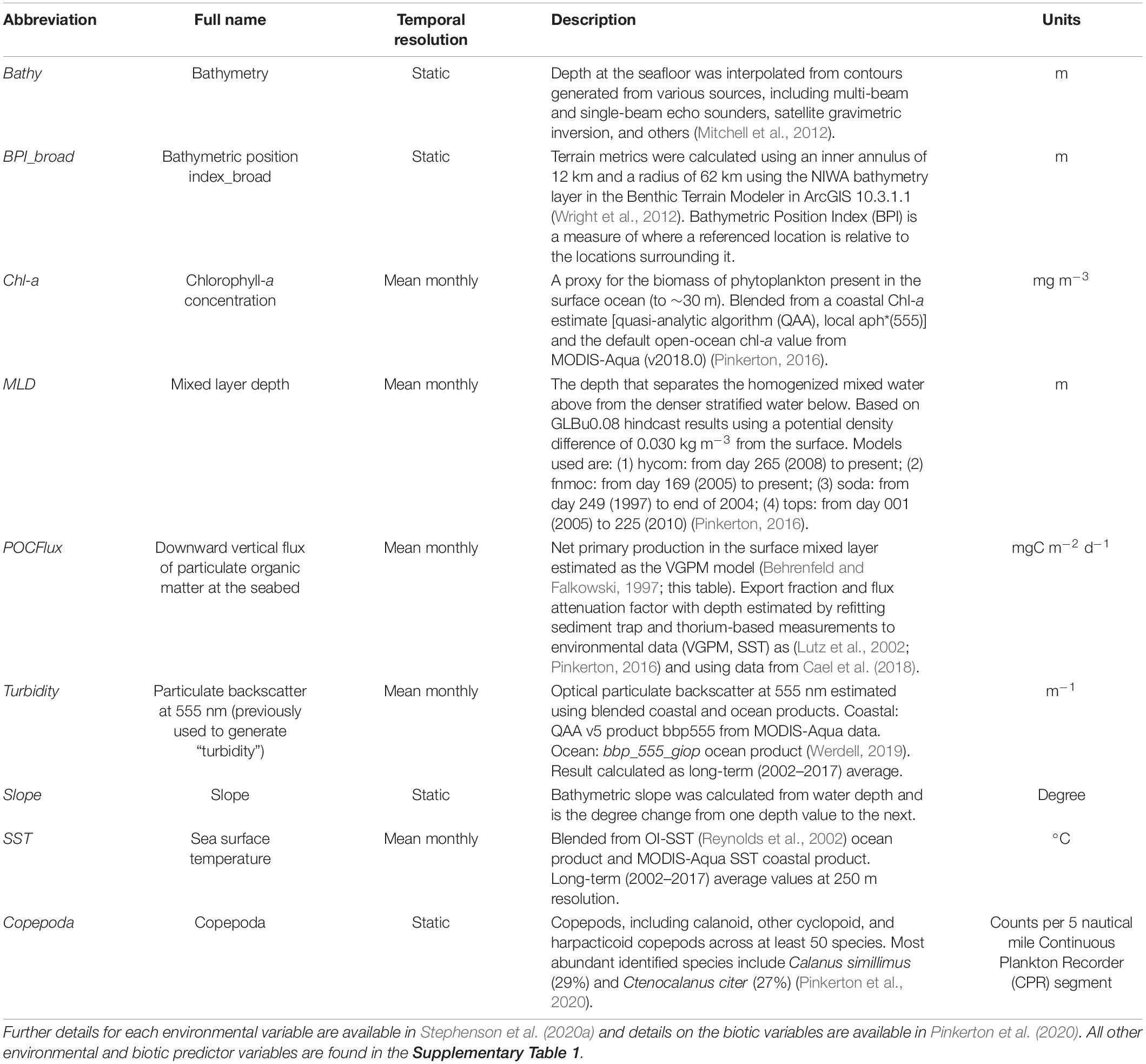
Table 1. Spatial environmental and biotic predictor variables included in the final models, collated for species distribution models from Stephenson et al. (2020a).

Of the available environmental and biotic variables, a subset was selected to be used in the models (Table 1) based on model tuning described in section “Predictor Variable Selection.” Although most of the chosen environmental variables were static (e.g., bathymetry, Bathy), several variables were dynamic in time, representing mean monthly statistics for the past 20 years (e.g., chlorophyll-a concentration, Chl-a, “temporal resolution” column in Table 1). The environmental data spans a much shorter timeframe than the basking shark observations (131 years), and thus, long-term trends in habitat suitability could not be examined. Prior to fitting of the habitat suitability models, values for each environmental and biotic variable were extracted for locations of basking shark records by overlaying the records onto each of the environmental and biotic variable layers using the “raster” package in R (Hijmans and van Etten, 2012). For dynamic environmental variables (mean monthly statistics), recorded dates of basking shark records were used to extract respective values from the month the record was made.

Habitat Suitability Modeling

Habitat Suitability Models (HSMs) were used to analyze and spatially predict the distribution of basking shark habitat suitability (measured as habitat suitability index—HSI). Acknowledging that our environmental predictors are mean (or mean monthly) averages for the past 20 years, we explored models for two time periods: 1889–2020 (all data, n = 369) and as subset of basking shark occurrence which matched the time frame of our environmental predictors 2000–2020 (n = 123). The relationship between environmental variables, biotic variables and basking shark records was explored using ensemble predictions (Ensemble HSM) from Boosted Regression Tree (BRT) and Random Forest (RF) models. This approach limits dependence on a single model type or structural assumption and may result in a more robust characterization of the predicted spatial variation and uncertainties (Robert et al., 2016). To estimate basking shark distributions, BRT and RF models require locations of both presences (occurrence records) and absences. Here, true absences (i.e., sample locations where no basking sharks were recorded) were not available for opportunistic records such as public sightings, media reports, or museum records. True absences were also unavailable for the non-opportunistic sampling methods (i.e., trawl tows, observer records, scientific surveys), particularly from commercial records which are complicated with the inclusion of multiple gear types and fishing protocols (thus affecting catchability) and issues regarding a lack of reporting of basking shark interactions (Francis, 2017). Therefore, presence only modeling approaches using pseudo-absences (i.e., locations where basking sharks were not recorded within our study area) were necessary.

Pseudo-Absence Selection

A two-dimensional kernel density estimate (KDE) was produced using all basking shark locations (presence data) using a cell size of 1 km² and a default bandwidth (Supplementary Figure 2). Within the KDE, the 95% percentage volume contour (minimum area in which 95% of the KDE value is located) was selected (Calenge, 2006). The 95% KDE was used to create a probability grid from which pseudo-absences were sampled according to the probability of grid weights (that is, where KDE values were high, the chance of selecting an absence was high) (Georgian et al., 2019). Pseudo-absences were generated through random selection of points from within the probability grid except within a 1 km²-grid radius of the presence localities. By selecting pseudo-absences in this manner, the pseudo-absences were subject to the same sampling bias as the presence data. This method has been shown to increase the accuracy of presence only BRT and RF models (Elith et al., 2010; Cerasoli et al., 2017; Georgian et al., 2019). Following recommended best practice, the number of pseudo-absences selected by month were equivalent to the number of monthly presences (Barbet-Massin et al., 2012).

Predictor Variable Selection

In most cases, the inclusion of many variables (e.g., >20 variables) in tree-based machine learning models (i.e., BRT and RF) is avoided because they only provide minimal improvement in predictive accuracy, and complicate interpretation of model outcomes (Leathwick et al., 2006). As the interpretation of drivers of distribution of basking shark was a key requirement, a reduction in the number of predictor variables was undertaken in order to produce a parsimonious model. A BRT model was initially fitted using all available environmental variables which was then subjected to a simplification process whereby environmental variables were removed from the models, one at a time, using the “simplify” function (Elith et al., 2006). This simplification process firstly assesses the relative contributions of each variable in terms of deviance explained, with the lowest contributing variables removed from the model. The model is then refitted with the remaining environmental variables. The change in deviance explained that resulted from removing the variable was then examined and the process repeated until the deviance explained decreased by >1% between removal of predictor variables. Despite having a relatively small influence on the model, Chl-a was retained as this predictor was found to be an important predictor of basking shark distribution elsewhere (Austin et al., 2019).

The final variables retained for modeling were Bathymetry, BPI broad, Chl-a, mixed layer depth (MLD), Turbidity, POCFlux, Slope, and SST (Table 1), as well as Copepoda, a known prey species for basking sharks (Grieve, 1966). Several environmental variables showed some co-linearity (Supplementary Figure 3) however, all levels of co-linearity were considered acceptable for tree-based machine learning methods (Pearson correlation < 0.75; Elith et al., 2010; Dormann et al., 2013). The “final” environmental variables selected through this approach were also used in RF models (Supplementary Table 1 and Supplementary Figures 1.1–1.8). Partial dependence plots were made for the BRT and RF models to evaluate the effect of each predictor on species’ distribution by plotting the effect of the predictor on the response (basking shark presence) after accounting for the average effects of all other model predictors (Elith et al., 2008).

Boosted Regression Tree Models

BRT modeling combines many individual regression trees (models that relate a response to their predictors by recursive binary splits) and boosting (an adaptive method for combining many simple models to give improved predictive performance) to form a single ensemble model (Elith et al., 2008). Detailed descriptions of the BRT method are available in Ridgeway (2007) and Elith et al. (2008). All statistical analyses were undertaken in R (R Core Team, 2020) using the “Dismo” package (Hijmans et al., 2017). BRT models were fitted with a Bernoulli error distribution, a tree complexity of 2, a learning rate of 0.01 (with parameters selected so as to fit trees for each bootstrapped model), a bag fraction of 0.7 and random 10-fold cross evaluation following recommendations from Leathwick et al. (2006) and Elith et al. (2008). The BRT method has been widely used in ecological applications and has performed well in previous studies of fish, zooplankton, and cetacean distributions in New Zealand (Leathwick et al., 2006; Compton et al., 2013; Pinkerton et al., 2020; Stephenson et al., 2020b).

Random Forest Models

RF models fit an ensemble of regression (abundance data) or classification tree (presence/absence data) models describing the relationship between the distribution of an individual species and some set of environmental variables (Ellis et al., 2012). Following environmental and biotic predictor variable selection using the BRT model, RF models were fitted using the R package “randomForest” (Breiman, 2001) and were tuned using the train function in the R package “caret” (Kuhn et al., 2020). The train function selects optimal values for the complexity parameters mtry (the number of variables used in each tree node), maxnodes (the maximum number of terminal nodes in each trees), and ntree (the number of trees to grow).

Bootstrapping the Models

BRT and RF models were bootstrapped 200 times. A random “training” sample with a sample size equal to the number of presence records was drawn with replacement. A random sample of pseudo-absences of equal number was drawn without replacement from the full set of available pseudo-absences stratified by month (to match the monthly environmental data) (Barbet-Massin et al., 2012) and the models were run using these presence-pseudo absence records. Presence records which were not randomly selected were combined with a random number of pseudo-absences and were set aside for independent assessment of model performance (referred herein as “evaluation” data). At each BRT and RF model iteration, geographic predictions were made using environmental predictor variables to a 1 km² grid. Given that BRT and RF models used pseudo-absences, we refer to our outputs as “habitat suitability” (rather than the commonly used “probability of occurrence”) because we did not have information on “catchability” or “sightability” of basking sharks from the different sampling methods nor did we have estimates of species prevalence (Anderson et al., 2016; Georgian et al., 2019). HSI and a spatially explicit measure of uncertainty (measured as the standard deviation of the mean predicted HSI) were calculated for each grid cell using the 200 bootstrapped layers.

Model Performance

BRT and RF model performance were evaluated using AUC (area under the Receiver Operating Characteristic curve) and TSS (True Skill Statistic). AUC is an effective measure of model performance and a threshold-independent measure of accuracy, while the TSS is a threshold-dependent measure of accuracy, but is not sensitive to prevalence (Allouche et al., 2006; Komac et al., 2016). AUC scores range from 0 to 1, with a score of 0.5 indicating model performance is equal to random chance, a score > 0.7 indicating adequate performance, and a score > 0.80 indicating excellent performance (Hosmer et al., 2013). TSS, which takes into account Specificity (correct prediction of absence) and Sensitivity (correct prediction of presence) to provide an index ranging from –1 to +1, where +1 equals perfect agreement and –1 is no better than random, Allouche et al. (2006). A TSS value > 0.6 is considered useful (Allouche et al., 2006). Model fit metrics were calculated using both the “training” dataset and the “evaluation” dataset. The latter is considered a more robust and conservative method of evaluating goodness-of-fit of a model than using the same data with which the model was trained (Friedman et al., 2001).

Ensemble Models

We produced an ensemble model by taking weighted averages of the predictions from each model type, using methods adapted from Anderson et al. (2016, 2020) and Georgian et al. (2019). This adapted procedure derives a two-part weighting for each component of the ensemble model, taking equal contributions from the overall model performance (AUC value derived from the “evaluation”) and the uncertainty measure (SD) in each cell, as follows:

{W1}_{BRT} = \frac{{AUC}_{BRT}}{{AUC}_{BRT} + {AUC}_{RF}} and W 1_{R F} = \frac{A U C_{R F}}{A U C_{B R T} + A U C_{R F}}

{W2}_{BRT} = 1 - \frac{{SD}_{BRT}}{{SD}_{BRT} + {SD}_{RF}} and W 2_{R F} = 1 - \frac{S D_{R F}}{S D_{B R T} + S D_{R F}}

W_{BRT} = \frac{{W1}_{BRT} + {W2}_{BRT}}{2} and W_{R F} = \frac{W 1_{R F} + W 2_{R F}}{2}

X_{ENS} = X_{BRT} * W_{BRT} + X_{RF} * W_{RF}

{SD}_{ENS} = {SD}_{BRT} * W_{BRT} + {SD}_{RF} * W_{RF}

where AUC_BRT and AUC_RF are the model performance statistics; X_BRT and X_RF are the model predictions; SD_BRT and SD_RF are the bootstrap SDs; and X_ENS and SD_ENS are the weighted ensemble predictions and weighted SDs, respectively, from which maps of predicted species distribution and model uncertainty were produced.

Measures of Uncertainty

Two measures of spatially explicit uncertainty were produced: an estimate of our spatial coverage of species occurrence (95% KDE) and the standard deviation of the predicted basking shark distribution (i.e., model uncertainty). The calculated spatial coverage of species occurrence was assumed to be indicative of basking shark distributions, and thus, is presumed to have more certain predictions of the species’ distribution of suitable habitat. Where predictions were projected outside the spatial coverage of species occurrence (i.e., where there are few or no sightings), it is assumed that the relationship between the environment and species’ records may be less robust and thus predictions outside this range contain some degree of uncertainty (e.g., similarly to the methods used in Stephenson et al., 2020b). Standard deviation (SD) of the mean predicted habitat suitability were estimated through the bootstrapping methods outlined in section “Bootstrapping the Models” and are provided as uncertainty estimates of basking shark distribution.

Ensemble model performance was assessed using AUC and TSS by comparing ensemble model predictions to all basking shark presence records and an equal number of randomly selected pseudo-absence data. To ensure that the random selection of pseudo-absence data did not provide misleading model performance metrics, this procedure was iterated 50 times and mean AUC and TSS score calculated for the ensemble model (Barbet-Massin et al., 2012). Ensemble partial dependence plots were created with an average of the BRT and RF partial dependence plots.

Model performance and outputs for the two time-series were found to be very similar and the outputs for the longer time series (1889–2020) are reported in the Results. The final model shown here is a temporally and spatially smooth prediction of basking shark HSI in New Zealand waters. By including all available data points, the model has retained a substantial amount of the New Zealand environment, including areas known to be historically important for basking sharks (e.g., east coast of the South Island). Inclusion of historical data across a long temporal span has been shown to achieve the highest model performance in SDMs, particularly when presence-only data is available (Lütolf et al., 2006). Model performance, partial dependence plot and predicted habitat suitability for the shorter time series (2000–2010) are found in the Supplementary Table 2 and Supplementary Figures 8, 9).

Results

Basking Shark Records

Of the records retained for use in the models, most basking shark records (72%, n = 265) occurred in the spring and summer months (September to February). Most (69%) records came from fishing interactions (trawl = 244, set net = 7, surface longline = 3), followed by public sightings (13%, n = 47), aerial surveys (11%, n = 41), research vessels (4%, n = 14), and alternative capture methods (e.g., harpoon) or unknown sources (4%, n = 13). Since 2000, most records (84%, n = 103) have been from fishing events, with one aerial record and 19 opportunistic sightings. The most recent coastal sighting and coastal fishing interaction (set net) occurred in March 2012 and August 2014, respectively, and the last known report of a school (≥3 individuals) was from April 2013 where seven individuals were captured in one trawling event. Estimated lengths were available for 169 records (42%); 32 records were <5 m (19%), 126 records were 5–10 m (74.5%), and 11 records were >10 m (6.5%) (Supplementary Figure 4). For observations where length was recorded, sex was available for 81 of these records (20% of all basking shark observations). Most sharks (89%, n = 72) were male and nine (11%) were female (Supplementary Figure 5).

Model Performance

AUC and TSS scores using evaluation data were very similar between models, with the RF model performing slightly better than the BRT model (AUC: 0.92 and 0.89; TSS: 0.72 and 0.69, respectively, Table 2). Both indices indicated the models were useful in predicting basking shark occurrence (>0.7). Measures of BRT and RF model performance scores had low variability (measured by the standard deviation of the mean), suggesting the models were performing consistently across bootstrap samples. Model fits between training data and evaluation data were similar, with model fits for the evaluation data slightly lower than the training data (as would be expected). The similarity of these fits provides some indication that the training data were not overfitted in the models.

TABLE 2

Table 2. Mean cross-validated estimates of model performance for the bootstrapped boosted regression tree (BRT) and random forest (RF) models (time series 1889–2020).

Variable Selection and Contribution

The relative importance of each predictor and their influence on basking shark habitat suitability were consistent across BRT and RF models (Supplementary Figures 6, 7). The three most important variables in predicting basking shark habitat suitability were vertical flux (POCFlux, with 26.0% influence on the response), slope (Slope, 14.1%), and turbidity (Turbidity, 10.6%) (Figure 2). Bathymetry (Bathy, 9.7%) and BPI broad (BPI broad, 9.6%) were also moderately important variables. There was a strong positive relationship of predicted basking shark HSI with vertical flux, highest in areas where vertical flux was 20 mgC m^–2 d^–1 or greater than what would be expected for the given depth. High HSI was predicted in gently sloping and less complex seafloor topographies with moderate turbidity. Two depth strata had high HSI—nearshore depths and depths between 200 and 550 m. A less clear relationship was observed between HSI and SST and mixed layer depth (MLD), with low HSI occurring between temperatures of 12.5 and 15°C and in areas where the mixed layer depth was approximately 75 m. There was a weak relationship between HSI and copepod (Copepoda) densities, with low HSI occurring with low levels of copepod densities, a peak in HSI at moderate copepod densities (10–20 counts per 5 nautical miles), and a plateau in HSI values at the highest levels of copepod densities (>25 counts per 5 nautical miles). HSI was lowest at moderate levels of chl-a concentration (Chl-a) (0.5–1.0 mg m^–3) and highest at high chl-a concentration (>1.2 mg m^–3).

FIGURE 2

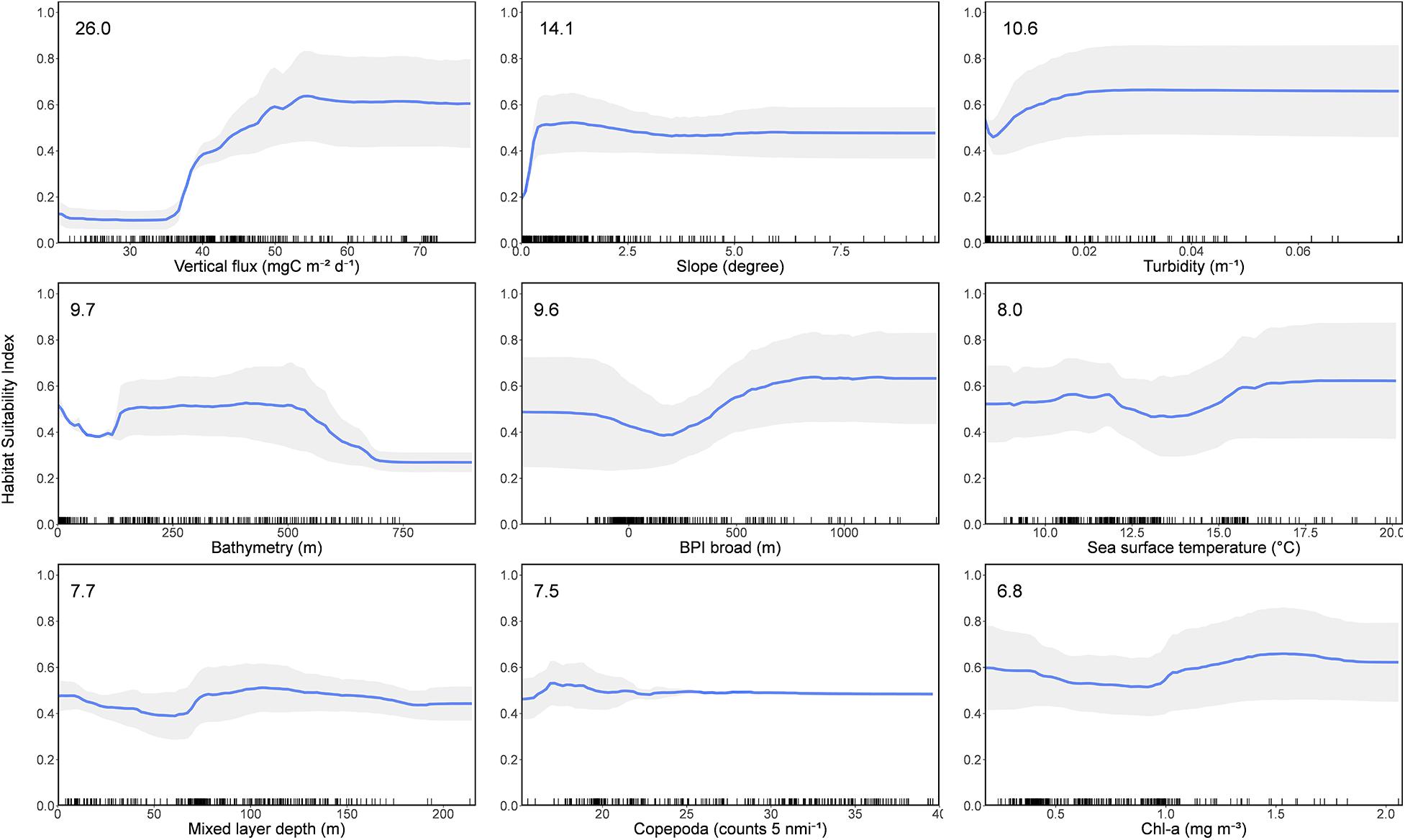
Figure 2. Partial dependence plots of the mean boosted regression tree (BRT) and random forest (RF) models for the nine variables (time series 1889–2020), showing the influence of each predictor variable on the response. Variables are ordered by influence as indicated in top left hand of plots. Shaded area represents standard deviation.

Predicted Basking Shark Distributions

Areas of predicted high habitat suitability for basking sharks in New Zealand waters occurred along the continental slope, particularly along the 250 m contour along the North and South Islands, Mernoo Bank, Pukaki Rise, Puysegur Ridge, and around New Zealand’s offshore islands (Chatham Islands, Stewart Island, Bounty Islands, and Auckland Islands) (Figures 3, 4). Within the spatial coverage of species occurrence, areas of moderate uncertainty (SD > 0.2) included most offshore waters north of 40°S, the deeper depths (>500 m) of the Hokitika Canyon, northern Chatham Rise, coastal waters off east coast of the South Island (Canterbury Bight), Foveaux Strait and Puysegur Ridge (Figure 5). The northern North Island and features further from the continental shelf, including the eastern half of the Chatham Rise were outside of the estimated spatial coverage (95% KDE) of species occurrence. In addition, moderate—high uncertainty (SD > 0.2) was reported along deep sea features north of New Zealand, including the Kermadec Ridge and Trench, the Lau-Colville Ridge, and the Norfolk Ridge (Figure 5).

FIGURE 3

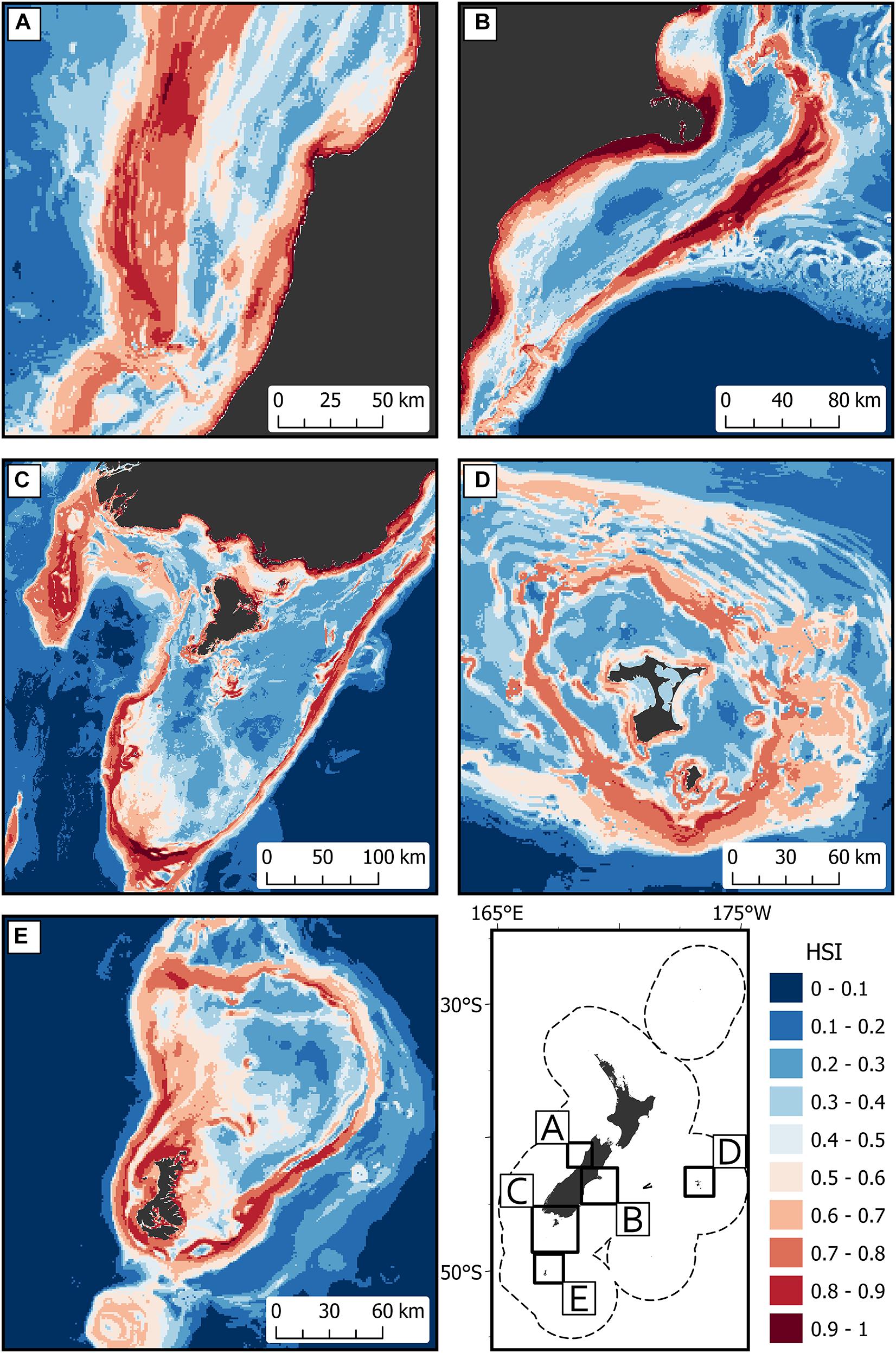
Figure 3. The predicted habitat suitability index (HSI) of basking shark in the New Zealand Exclusive Economic Zone (EEZ) from 1889 to 2020 modeled using the bootstrapped ensemble models for (A) west coast South Island; (B) east coast South Island; (C) south of South Island including Puysegur Ridge and Stewart Island; (D) Chatham Islands; and (E) Auckland Islands. Areas outside 95% kernel density estimate (KDE) probability grid indicating lower confidence that can be placed in the predicted probability occurrence are covered by crossed black lines. Note that the Chatham Islands (D) is outside the KDE probability grid estimate.

FIGURE 4

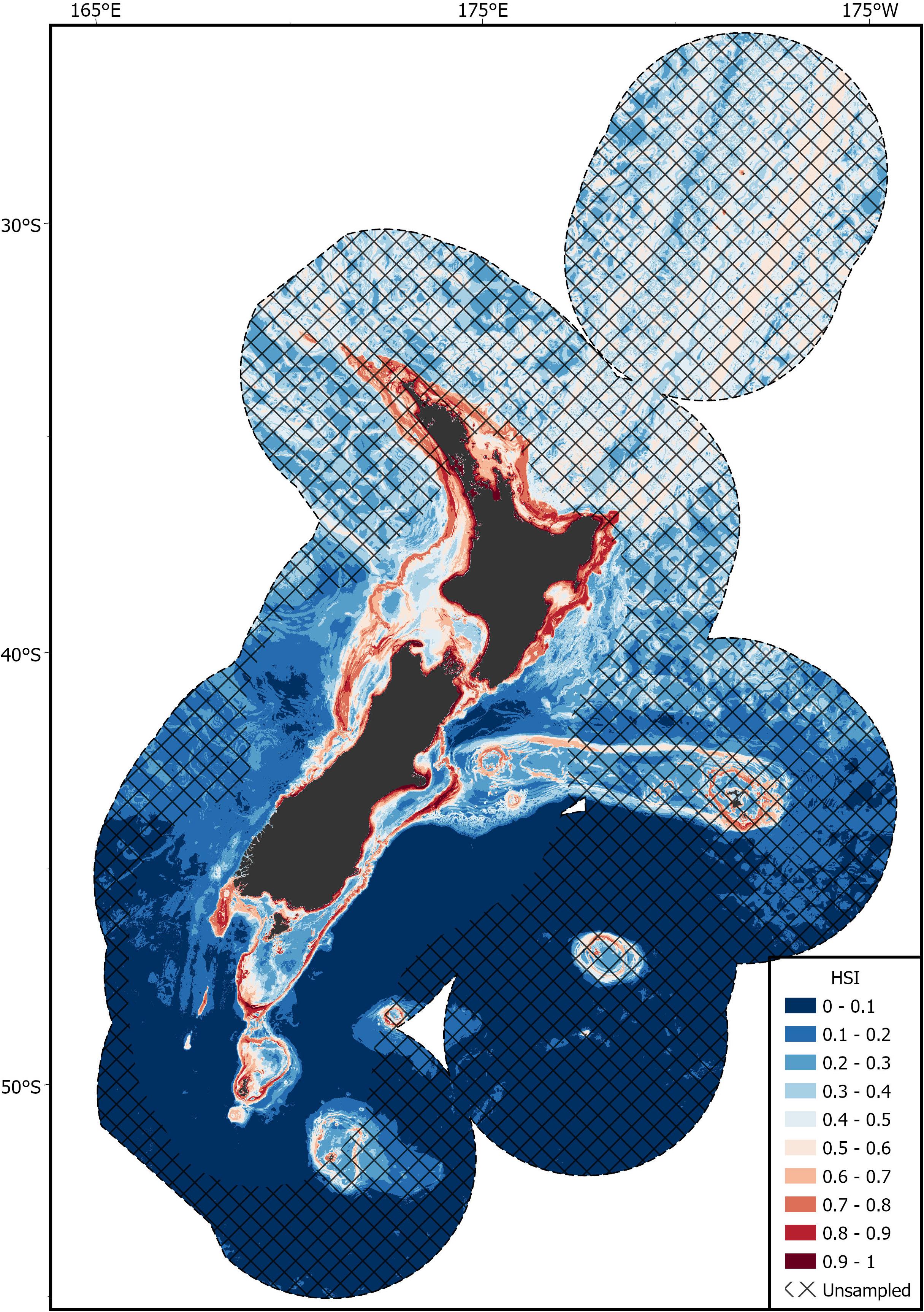
Figure 4. The predicted habitat suitability index (HSI) of basking shark in the New Zealand Exclusive Economic Zone (EEZ) from 1889 to 2020 modeled using the bootstrapped ensemble models. Areas outside 95% kernel density estimate (KDE) probability grid indicating lower confidence that can be placed in the predicted probability occurrence are covered by crossed black lines.

FIGURE 5

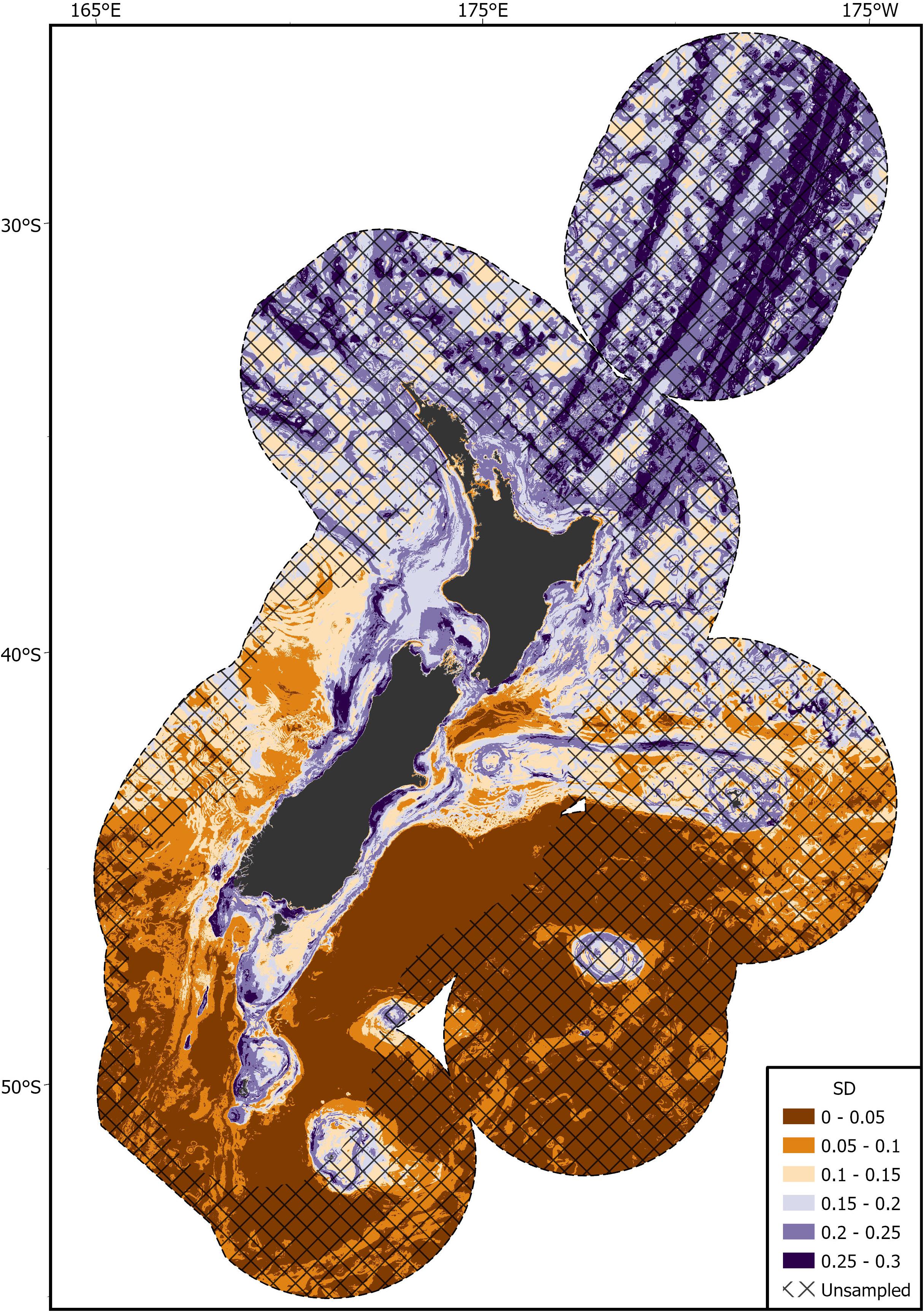
Figure 5. Standard deviation (SD) of the predicted habitat suitability index (HSI) of basking shark in the New Zealand Exclusive Economic Zone (EEZ) from 1889 to 2020 modeled using the bootstrapped ensemble models. Areas outside 95% kernel density estimate (KDE) probability grid indicating lower confidence that can be placed in the predicted probability occurrence are covered by crossed black lines.

Discussion

This study has provided the first insight into habitat suitability for basking sharks in the Southwest Pacific. Our approach assessed habitat suitability by incorporating a combination of static and temporally dynamic environmental (n = 7), biotic (n = 1), and inferred prey (n = 1) predictors into ensembled HSI models. The BRT and RF models had good predictive power (AUC and TSS > 0.7) and both models performed similarly with low variability in the model fit metrics. The outputs produced here will be useful for fisheries risk assessment (e.g., spatially explicit risk assessment), as well as providing guidance for future research efforts (e.g., areas of interest for future sampling). However, caution should be considered given the relatively few species presence records and lack of true absence data.

Drivers of Predicted Basking Shark Distribution

Basking shark habitat suitability was largely influenced by variables representing ocean processes. The environmental predictors used in this work were comprehensive and many were dynamic (i.e., monthly means were available). Overall, areas with high levels of vertical flux of particulate organic matter at the seabed had high habitat suitability. This is likely indicative of higher levels of primary production in the surface ocean and higher prey density in the mesopelagic zone and at the seafloor and may be a suitable proxy when prey data is unavailable. The biotic predictive layers included here were found to have lower influence on habitat suitability compared to some of the environmental predictors. However, prey availability is highly patchy and temporally variable; thus, it is likely that a static variable reflecting prey abundance was unable to accurately represent the spatial distribution of prey. The inclusion of biotic predictors in the model is important in understanding species’ relationship with the marine environment in unobserved space and has been identified as a potential link in understanding effects of climate change. In the Northeast Atlantic, basking sharks are often observed in shallow, highly productive coastal waters during spring and summer months where they feed on zooplankton blooms (Sims, 2008). Historically, basking sharks were commonly observed in similar environments (e.g., east coast of the South Island) around New Zealand (Francis and Duffy, 2002). Although prey preference for New Zealand sharks is poorly understood, there is some relationship between New Zealand basking shark distribution and copepod abundance, as seen in the North Atlantic (Sims and Merrett, 1997).

The inclusion of dynamic (mean monthly) environmental variables here may allow the models to capture temporal change in patterns of basking shark distribution, including seasonal changes and interannual variability. Despite the availability of dynamic environmental predictors, true temporal changes in distribution are difficult to confirm due to the limited amount of biological data (basking shark observations) available. However, in our results, both inshore and offshore regions were highlighted as areas of high habitat suitability. This is particularly evident in the bimodal effect of the bathymetry predictor, where basking shark habitat suitability was observed to be highest in very shallow depths (<100 m), and again at depths between 200 and 500 m. This result is consistent with previous work where basking sharks have been shown to exhibit seasonal vertical space use in the Northeast Atlantic, with tagged individuals occupying shallow depths (<100 m) in the summer months and depths greater than 1,000 m in late winter/early spring (Doherty et al., 2019).

While bathymetry (and slope) were also found to be important predictors, their effect may be partially influenced by basking shark availability to fisheries (see below). Basking sharks have been shown to dive as deep as 1,264 m and have been regularly documented at depths of 600–1100 m (Francis and Duffy, 2002; Gore et al., 2008; Doherty et al., 2017). The species has also been shown to follow distinct water masses at depth, remaining at depths of 250 m or more for months without coming to the surface (Braun et al., 2018; Dewar et al., 2018). Basking sharks are known for complex diel vertical movements, which are thought to be influenced by shifts in prey availability and oceanography (Sims et al., 2005; Dewar et al., 2018). In well-stratified deep waters, basking sharks exhibit normal diel vertical movements (shallow depths at night, deeper depths during daylight), while sharks occupying inshore, inner-shelf areas near thermal fronts conduct reverse diel vertical movements (shallow depths during the day, deeper depths at night) (Sims et al., 2005). This may explain, at least in part, why more contemporary reports of basking sharks in deepwater fisheries have been made during daylight hours (when sharks are occurring at their preferred deeper depth range) but does not offer insight into the disappearance of inshore observations or why individuals are no longer seen at the surface in the region.

Water temperature had relatively minimal influence on basking shark distribution. Basking sharks appear to have a broad thermal range and are therefore relatively unrestricted by temperature (Sims et al., 2003). They are also known to cross tropical regions by submerging into deeper, colder water (Skomal et al., 2009), and one individual was encountered in tropical waters off Indonesia (Fahmi and White, 2015). While gradual changes in sea temperatures may have minimal effect on basking sharks, ocean heat waves and extreme processes associated with SSTs might be more relevant and are expected to become more prevalent with climate change. By 2100, climate change projections predict SST will increase by 2.5°C, which in turn is predicted to lead to a deepening in the surface mixed layer depth (by 15%), declines in primary production (4.5%) and particle flux (12%); the largest changes in macronutrients are predicted in eastern Chatham Rise and southern Sub-Antarctic waters (Law et al., 2018). Such changes may alter food availability (prey distribution and abundance) for basking sharks resulting in shifts in their distribution.

Predictors found to positively influence basking shark HSI could be further explored to better understand historic and future basking shark distribution. Predictors including chl-a concentration and vertical flux are often used as an index of phytoplankton abundance (primary production) and are strongly linked to primary consumers such as copepods. In recent decades, dramatic shifts in chl-a concentration have been reported in the South Pacific and the Southern Oceans (Del Castillo et al., 2019). Significant declines in chl-a concentration were observed in spring and summer months in the South Pacific from 1979 to 2000, while significant increases were linked to extreme summer marine heatwaves in the Southern Ocean between 2002 and 2018 (Gregg and Conkright, 2002; Montie et al., 2020). Highly variable oceanographic conditions around New Zealand are strongly correlated with climate phenomenon such as El Niño–Southern Oscillation (ENSO) (Bradford-Grieve et al., 2006). In the Northern Hemisphere, basking shark movement patterns have been linked to shifts in prey availability and oceanography (Sims et al., 2005; Gore et al., 2008; Dewar et al., 2018). One tagged individual was shown to remain in an area with putative upwelling and high abundance of phytoplankton in the Western Atlantic for up to a month (Gore et al., 2008). In the Northeast Atlantic, a northward shift in basking shark distribution in response to long-term zooplankton declines was found to correspond with declines in basking shark catch in Irish fisheries to the south from 1948 to 1975 (Sims and Reid, 2002). Similar models used in this project could be explored to predict basking shark distribution response to future climate change forecasting and events such as ENSOs [e.g., Earth System Models, Anderson et al. (2020)].

Basking Shark Habitat Suitability in New Zealand

Areas of high basking shark habitat suitability included the east and west coasts of the South Island, Puysegur Ridge, and the Auckland Island slope. Some areas of Chatham Rise, specifically around Mernoo Bank (including Mernoo Saddle) and off the southern slope of Pitt Island (Chatham Islands), were also identified as areas of high habitat suitability. Much of Chatham Rise, however, was outside the spatial coverage of species occurrence and thus habitat suitability predictions hold a higher degree of uncertainty. Chatham Rise is a known hotspot for chondrichthyan diversity in New Zealand waters (Wetherbee, 2000), but interestingly, basking sharks have very rarely been reported from the area. Chatham Rise, as well as Puysegur Ridge, have relatively low densities of copepods (see Supplementary Figure 1.9) and may not be optimal feeding grounds for basking sharks. However, in international waters east and north-east of Chatham Rise, 15 juvenile basking sharks (180–310 cm total length) were reported by Japanese drift net vessels operating at shallow depths (10 m) (Yatsu, 1995). This report suggests juvenile sharks may inhabit epipelagic waters in the open ocean (Francis, 2017).

Given the long temporal span of the data, model predictions may be more representative of past, rather than current habitat suitability, particularly some inshore parts of the predicted distribution. Basking sharks are occasionally recorded from northern New Zealand and were reported to be regular visitors to the Hauraki Gulf during spring in the late nineteenth century (Cheeseman, 1891). The predictions presented here are smoothed over time, as there is a mismatch between the availability of basking shark records (131 years) and environmental data (approximately 20 years). It is possible that the models have highlighted seasonal patterns of distribution by indicating both inshore and offshore regions as areas of high habitat suitability with the presence of bimodality in the bathymetry HSI. However, these patterns could also be indicative of a shift to deeper, offshore habitats in recent decades.

There were several areas where the spatially explicit uncertainty (measured as the SD) was relatively high, indicating the relationship between basking sharks and the environment was more uncertain. Our understanding of basking shark use of the pelagic habitat remains relatively unknown, largely due to the spatial bias in observations (e.g., lack of open ocean pelagic research surveys). In areas with high uncertainty, such as Cook Strait, the northern Chatham Rise, and Foveaux Strait, few basking shark sightings where available and uncertainty might be linked to low sample size. Uncertainties regarding the most northern predictions of habitat suitability (north of 40°S) may, in part, be explained instead by a lack of information on copepod density north of 40°S (Pinkerton et al., 2020), but is more likely associated with a lack of basking shark data. Despite a lack of surface sightings around northern New Zealand, there is some evidence of basking shark captures in deepwater trawl fisheries off central Hawke’s Bay. Basking sharks may be present along the upper slope around northern New Zealand but there is no fisheries-independent data (research or public sightings) to indicate their presence. In the Kermadec Islands where there is minimal human presence, there is one unconfirmed stranding of a basking shark from Raoul Island (Morton, 1957).

The estimate of spatial coverage of species occurrence (top 95% of the KDE of basking shark occurrences) provides a representation of the likely geographic (and in turn environmental) space occupied by basking sharks within New Zealand waters. Predicted distribution outside of this area, should be treated with caution as this represents prediction into largely unsampled space. In this study, the environmental threshold reflects the distribution of presences only—and thus retains any spatial biases associated with these datasets. In particular, the spatial distribution of presences is related to the distribution of fishing effort and human population centers (for opportunistic sightings) and may not be an accurate representation of hotspots. However, using the top 95% of the KDE of basking shark occurrences provides a more conservative estimate of this species’ spatial distribution, which can be useful in determining when modeled predictions are occurring outside of sampled environmental space. This measure provides a meaningful threshold with which to classify broad areas as “uncertain.”

Future Directions

The lack of basking shark records in New Zealand waters during recent years highlights the need to better understand their overall abundance, distribution, movements, and habitat use in the South Pacific Ocean as well as changes to the sighting effort. Currently data collection on the species in the Southern Hemisphere is heavily reliant on interactions with fisheries, especially trawl fisheries (Francis and Smith, 2010; Hernández et al., 2010; Lucifora et al., 2015; Francis, 2017). Because of this, our knowledge of New Zealand basking shark distribution is essentially limited to areas of relatively high historic and current trawl fishing effort (Clarke et al., 2017; Baird and Wood, 2018). Most basking shark interactions occur during the spring-summer months, corresponding to when fishing vessels target commercially important species, such as spawning aggregations of arrow squid (Nototodarus sloanii) (Hurst et al., 2012). As a protected species, it is mandatory to report basking shark interactions with fisheries. However, there is uncertainty in the levels of reporting, and observer coverage is relatively low in some fisheries (e.g., inshore fisheries), particularly around northern New Zealand, so that presence records are likely underestimated (Francis, 2017). Understanding habitat use will assist in assessing risk to fishing activities and could be incorporated into management frameworks such as the spatially explicit risk assessment that New Zealand has in place for other protected species (Large et al., 2019).

Identifying areas of high habitat suitability could also assist in decision making processes for future research efforts. Previous research has identified the need to tag free-swimming basking sharks to better understand species movement, habitat use, and interactions with fisheries (Francis, 2017). This will require the ability to find individuals at the surface, and at an accessible location. Meeting these requirements has prevented any efforts of tagging New Zealand basking sharks to date. In the Atlantic Ocean, basking sharks have been successfully tagged off Cape Cod, Massachusetts and the west coast of Scotland and Isle of Man (Skomal et al., 2009; Doherty et al., 2017; Hawkes et al., 2020) and in the Pacific, off San Diego and Monterey Bay, California (Dewar et al., 2018). By identifying areas of high habitat suitability, research efforts can be directed to specific areas of interest to increase the tagging success. For example, the Auckland Islands has been identified as an area of high habitat suitability for basking sharks where basking sharks were historically sighted at the surface (Parrott, 1958). This area is also a known hotspot for other large filter-feeding vertebrates that feed along the Subtropical Front (STF), a continuous feature within the Southern Tropical Convergence at latitudes 39°–42°S, characterized by elevated primary productivity (Murphy et al., 2001; Rayment et al., 2015; Mackay et al., 2020). Southern Ocean oceanographic fronts have been identified as important foraging areas for a range of marine predators (Bost et al., 2009) and may also be important for basking sharks.

Differences in habitat suitability among sexes or size classes, a common observation among sharks, were not examined at this time due to the relatively small sample size of basking sharks across the region and low availability of size and sex data for most records. This information is becoming more readily available through fisheries observer data collection and should be explored further in the future. New Zealand has a considerable number of records of small (<5 m) sharks, accounting for nearly 20% of records where length has been recorded. Some of the most recent reports of basking sharks in New Zealand waters have been juvenile individuals, including a 3 m female captured east of the Auckland Islands in January 2018 and a 3.3 m male captured off the west coast South Island in August 2020. Both individuals were released alive. Continued collection of biological data on basking sharks is essential for understanding differences in habitat use across life history stages, particularly for juvenile basking shark as they are globally rare and their habitat preference is unknown.

More data on at-sea distribution of basking sharks is required to understand habitat use, threat overlap, and population status throughout the New Zealand and South Pacific region. The total South Pacific basking shark population size is unlikely to be high; in the Northeast Atlantic, basking shark numbers likely do not exceed 10 000 individuals (Lieber et al., 2020). With little population differentiation across global regions, it is plausible that basking sharks observed in New Zealand waters engage in large scale intra- and inter-oceanic migrations (Lieber et al., 2020). This may make species’ detection more difficult in the vast marine space of New Zealand’s EEZ. In the past, aerial surveys have been successful in detecting basking sharks distributed over relatively large spatial scales in New Zealand, and elsewhere for estimating regional population sizes (Francis and Duffy, 2002; Westgate et al., 2014). However, surveys conducted in 2010–2011 off Banks Peninsula failed to locate any basking sharks (Chapman and Duffy, 2011). These surveys have not been repeated since. Basking sharks may travel or feed in subsurface habitat, and therefore go undetected in aerial surveys. Alternative means of tracking these animals, such as autonomous underwater vehicles (AUV) (Hawkes et al., 2020) offer great potential for the future.

Data Availability Statement

The raw data supporting the conclusions of this article will be made available by the authors, without undue reservation, to any qualified researcher.

Author Contributions

CD and FS conceived the project. BF, FS, MF, CD, and MP collected the data. BF and FS analyzed the data and wrote the draft manuscript. GP created the maps. All authors discussed the results, contributed to the final manuscript, and approved the submitted version.

Funding

This project was funded by the Department of Conservation, Wellington, New Zealand (project CSP POP2020-03).

Conflict of Interest

The authors declare that the research was conducted in the absence of any commercial or financial relationships that could be construed as a potential conflict of interest.

Acknowledgments

Thanks to Jade Maggs (NIWA) and Fisheries New Zealand (FNZ) RDM for data extractions. Thank you to Ben Sharp (FNZ) for feedback on the methods. Satellite data are used courtesy of NASA (MODIS, SeaWiFS ocean color) and NOAA (AVHRR, sea-surface temperature). Mixed-layer depth data are used courtesy of Oregon State University “ocean primary productivity” project.

Supplementary Material

The Supplementary Material for this article can be found online at: https://www.frontiersin.org/articles/10.3389/fmars.2021.665337/full#supplementary-material

References

Aiello-Lammens, M. E., Boria, R. A., Radosavljevic, A., Vilela, B., and Anderson, R. P. (2015). spThin: an R package for spatial thinning of species occurrence records for use in ecological niche models. Ecography 38, 541–545. doi: 10.1111/ecog.01132