Integrated Assessment of Ocean Acidification Risks to Pteropods in the Northern High Latitudes: Regional Comparison of Exposure, Sensitivity and Adaptive Capacity

Exposure to the impact of ocean acidification (OA) is increasing in high-latitudinal productive habitats. Pelagic calcifying snails (pteropods), a significant component of the diet of economically important fish, are found in high abundance in these regions. Pteropods have thin shells that readily dissolve at low aragonite saturation state (Ω_ar), making them susceptible to OA. Here, we conducted a first integrated risk assessment for pteropods in the Eastern Pacific subpolar gyre, the Gulf of Alaska (GoA), Bering Sea, and Amundsen Gulf. We determined the risk for pteropod populations by integrating measures of OA exposure, biological sensitivity, and resilience. Exposure was based on physical-chemical hydrographic observations and regional biogeochemical model outputs, delineating seasonal and decadal changes in carbonate chemistry conditions. Biological sensitivity was based on pteropod morphometrics and shell-building processes, including shell dissolution, density and thickness. Resilience and adaptive capacity were based on species diversity and spatial connectivity, derived from the particle tracking modeling. Extensive shell dissolution was found in the central and western part of the subpolar gyre, parts of the Bering Sea, and Amundsen Gulf. We identified two distinct morphotypes: L. helicina helicina and L. helicina pacifica, with high-spired and flatter shells, respectively. Despite the presence of different morphotypes, genetic analyses based on mitochondrial haplotypes identified a single species, without differentiation between the morphological forms, coinciding with evidence of widespread spatial connectivity. We found that shell morphometric characteristics depends on omega saturation state (Ω_ar); under Ω_ar decline, pteropods build flatter and thicker shells, which is indicative of a certain level of phenotypic plasticity. An integrated risk evaluation based on multiple approaches assumes a high risk for pteropod population persistence with intensification of OA in the high latitude eastern North Pacific because of their known vulnerability, along with limited evidence of species diversity despite their connectivity and our current lack of sufficient knowledge of their adaptive capacity. Such a comprehensive understanding would permit improved prediction of ecosystem change relevant to effective fisheries resource management, as well as a more robust foundation for monitoring ecosystem health and investigating OA impacts in high-latitudinal habitats.

Introduction

The pervasiveness of global climate change threatens biodiversity, habitat suitability, ecosystem function, structure and services (Bindoff et al., 2019). Such changes are especially pertinent in high-latitudinal habitats across the eastern North Pacific Ocean, including the Gulf of Alaska (GoA) and its subpolar gyre, the polar waters of the Bering Sea, one of the most productive seas on the planet (Brown et al., 2011), and the Amundsen Gulf of the Canadian Beaufort Sea. Yet, the subpolar and polar seas are sensitive to ocean acidification (OA) due to naturally low buffering capacity, coupled with multiple climate-change and related physical-chemical drivers, such as increasing freshwater input from glacial runoff, rivers, sea ice melt, and increasing temperature (Mathis et al., 2011; Evans et al., 2013; Cross et al., 2013, Hauri et al., 2020). Substantial changes in carbonate chemistry conditions have already been detected, demonstrating increasing corrosiveness in high-latitudinal North Pacific regions (IPCC, 2014, 2019; Carter et al., 2017, 2019; Bindoff et al., 2019; Hauri et al., 2021). These changes coincide spatially and temporally with the habitats of important commercial and subsistence fisheries (Mathis et al., 2014), underscoring the need for a detailed understanding of the species tolerances and their habitats that will most likely be at risk. Currently, experimental data from the Pacific subpolar gyre, GoA, and Bering Sea show that economically important crab species (Long et al., 2013, 2016) and coho salmon (Williams et al., 2019) are sensitive to OA. However, very limited information exists from field measurements on the current impacts of OA on the most sensitive marine calcifying zooplankton (Cai et al., 2020), such as pteropods, with direct or indirect importance for the fisheries. Pteropods are a key species within the high-latitudinal ecosystems (Kobayashi, 1974; Fabry, 1989; Bednaršek et al., 2012a) that demonstrate severe sensitivity to OA. Multiple biological pathways of this species are impacted by OA conditions, compromising their growth, fecundity, and ultimately their survival (Comeau et al., 2009; 2010; Lischka et al., 2011; Bednaršek et al., 2014, 2019; Feely et al., 2016; Manno et al., 2016). As a result of such OA-related sensitivity, pteropods rank in the top quartile of ecological integrity indicators and are used to identify early warning signs and habitats of concern related to OA (Bednaršek et al., 2017).

Pteropods have a wide-ranging, year-around distribution in the subpolar gyre (Mackas and Galbraith, 2012), offshore and coastal habitats of the GoA (Tsurumi et al., 2005; Doubleday and Hopcroft, 2015), and Bering Sea (Eisner et al., 2014, 2017; Janssen et al., 2019), and the Amundsen Gulf (Darnis et al., 2008; Walkusz et al., 2013; Niemi et al., 2021). Pteropods in the GoA are commonly found in the diets of various life stages of Pacific Salmon species, such as pink, sockeye and chum salmon (Auburn and Ignell, 2000; Daly et al., 2019), that rely upon pteropods to support somatic growth and lipid reserves, especially during the critical summer and autumn growth periods (Auburn and Ignell, 2000; Armstrong et al., 2005; Beauchamp et al., 2007; Zavolokin et al., 2014; Doubleday and Hopcroft, 2015; Daly et al., 2019). They can also play a role in the diet of various fish in the Bering Sea, where high pteropod abundance occurs in the southern part of the basin, predominantly during the autumn (Eisner et al., 2014, 2017, 2017), making them one of the most dominant components of the diet of various salmon species (Zavolokin et al., 2007). In the Amundsen Gulf, pteropods comprise a small component of demersal Arctic cod diets (Majewski et al., 2016) and can be found at high numbers in the stomachs of coastal fish, including Arctic char (Niemi et al., 2021). In addition, given that pteropods in these regions have one of the highest abundances and biomass on the global scale, they also significantly contribute to the biological pump, especially to the carbonate flux (Bednaršek et al., 2012a). The most abundant species is Limacina helicina, which is present in two forms that are morphologically distinct from each other in the adult stage; one designated as L. helicina helicina, distinguished by an extended spire with striated surface, and the other as L. helicina pacifica, with a depressed (flat) spire and no striae present (McGowan, 1963; Janssen et al., 2019).

Assessing OA risks requires explicit linkages between three components (sensu Williams et al., 2008): (1) regional and local exposure to OA (e.g., changes in habitat suitability, spatial and temporal habitat change); (2) species’ sensitivity governed by intrinsic metabolic and ecological traits, such as climatic preferences, reproductive outputs, habitat use, and biotic and abiotic interactions; and (3) resilience and adaptive capacity (e.g., genetic and phylogenetic diversity, phenotypic plasticity, life history traits, dispersal potential, spatial connectivity). Emerging literature illustrates the species’ sensitivity under increasing OA exposure, but little is known about a vital component of the risk assessment: their distinct ecological, phenotypic or evolutionary specialization to changing conditions (e.g., Williams et al., 2008; Burridge et al., 2015).

Given the key role of pteropods in high-latitude ecosystems, there is an urgent need for an integrated assessment of OA risks for pteropod population viability in the high-latitudinal habitats, including the eastern part of the North Pacific, GoA, Bearing and Amundsen Gulf. Following Williams et al. (2008), we delineated pteropod OA risk assessment as a combination of exposure, sensitivity, and adaptive capacity. First, OA exposure was estimated using hydrographic observations and regional ocean biogeochemical models; we used model outputs to define short-term, seasonal OA exposure, as well as longer-term OA trends with the interannual and decadal changes that characterize a gradual OA intensification in the species’ exposure. These metrics of change offer tools to delineate the location of OA hotspots and habitat suitability with respect to OA, as well as temporal windows during which the biological exposure will be most significant.

Second, sensitivity was determined by observing early and well-defined negative effects of OA on pteropods, starting at aragonite saturation state (Ω_ar) values below 1.3 (Bednaršek et al., 2019), which is related to the shell biomineralization processes (dissolution and calcification). Such sensitivity was explored with respect to various morphotypes and matched with Ω_ar observations of the pteropods’ place of origin. Another important aspect of sensitivity is life history, specifically that of exposure severity as it co-occurs with varying levels of vulnerability over pteropod life stages.

Third, potential resilience was related to adaptive capacity, or phenotypic plasticity, genetic population structure, and population (spatial) connectivity. Genetic-based analyses can be used to identify cryptic species and their distribution and connectivity across all regions. Given limited knowledge about pteropod cryptic diversity (on the level of Limacina spp.) in the region, we focus our initial efforts on characterizing diversity at the species, subspecies, and morphotype levels (Maas et al., 2013; Gasca and Janssen, 2014; Sromek et al., 2015a,b; Shimizu et al., 2018, 2021). OA-induced exposure would not necessarily result in local vulnerability if individuals were replaceable. Evidence of co-occurring cryptic species or subspecies with differential response to OA might buffer changes in abundance. Similarly, large-scale spatial connectivity between geographic areas may promote replacement from unaffected areas.

Here, we conduct a comprehensive assessment of OA risks for the pteropod population in the eastern North Pacific Ocean and identify the areas of potential concern with respect to OA in the North Pacific subpolar gyre, GoA, Bering Sea, and Amundsen Gulf. We used a combination of high-resolution models, chemical observations, particle tracking and genetic surveys of species morphometrics to determine exposure, biological responses related to sensitivity, and resilience or adaptive capacity of pteropods to OA.

Methods

Physical-Chemical Seawater Characterization

Water samples for physical and chemical parameters were collected on the GO-SHIP P16N cruise (Figure 1A), the Dyson cruise in the Bering Sea (Figure 1B) and in the Amundsen Gulf (Canadian Beaufort Sea-Marine Ecosystem Assessment, or CBS-MEA; Figure 1C). Water was collected with a CTD/rosette package equipped with sensors for temperature (°C), salinity (PSU), and oxygen (μmol kg^–1), and a rosette of Niskin bottles for collecting discrete water samples throughout the water column. Dissolved oxygen was measured using titrations. Dissolved inorganic carbon (DIC) and total alkalinity (TA) samples were collected at discrete depths throughout the water column. In the Bering Sea, TA and DIC lab analyses were conducted on the water samples where pteropods were present. DIC and TA samples were collected in 250 ml borosilicate glass bottles and preserved with mercuric chloride following Dickson et al. (2007). DIC was measured using gas extraction and colorimetric titration with photometric endpoint detection (Johnson et al., 1998). TA was determined using open-cell potentiometric titration with a full curve Gran end-point determination (Haradsson et al., 1997). Certified Reference Materials (CRMs) were analyzed with both the DIC and TA samples as an independent verification of instrument calibrations (Dickson et al., 2007; Feely et al., 2016). Precision of measurements for DIC and TA was better than 0.1 % and 0.2 %, respectively. The saturation state of seawater with respect to aragonite was calculated from the DIC and TA measurements with the CO2SYS program (Lewis and Wallace, 1998) using the dissociation constants of Lueker et al. (2000) and the boron constant of Lee et al. (2010). Based on the uncertainties in the DIC and TA measurements and the thermodynamic constants, the uncertainty in the calculated Ω_ar was approximately 0.02. The Ω_ar observed values were correlated with the pteropod shell parameters (dissolution, density, thickness).

FIGURE 1

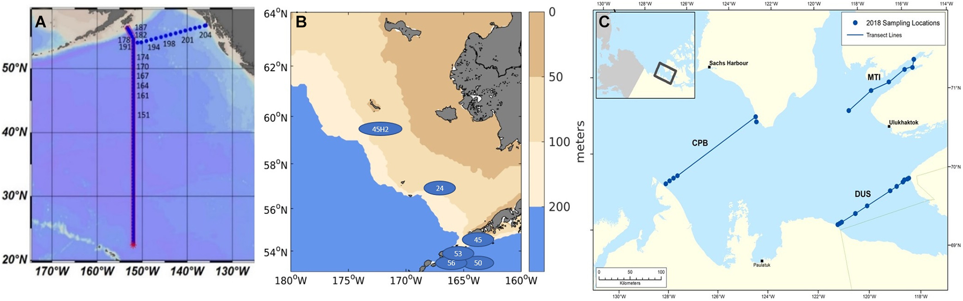
Figure 1. Biological samples taken in the Eastern pacific subpolar gyre and the GoA (A; samples analyzed from stations 164 to 204), and the Bering Sea (B; blue ellipses) and Amundsen Gulf (C) with three indicated transects related to the pteropod origin (Cape Bathurst (CPB), Dolphin and Union Strait (DUS), and Minto Inlet (MTI; see Niemi et al., 2021).

Pteropod Sampling

The list of stations where pteropods were collected, along with the data on abundance (reported in individuals per m²), shell morphological and genetic characteristics across all the investigated stations (North Pacific subpolar gyre, GoA, Bering Sea, Amundsen Gulf) are presented in Figure 1 and Table 1. Pteropods were sampled at 12 stations ranging from 48° to 56°N in the Gulf of Alaska and North Pacific subpolar gyre on the GO-SHIP P16N cruise in May and June 2015. Pteropods were collected using 202 and 335 μm mesh Bongo nets that were obliquely trawled for 20 min across the upper 100 m of the water column at night. Pteropod samples from the Bering Sea were obtained during an oceanographic survey by NOAA Alaska Fisheries Science Center (DY17-04 and DY17-08) in spring and summer (April and August) 2017. Samples were collected using 505 μm mesh net at six different stations. All pteropods were preserved in 100% buffered ethanol. Such sampling method does not accurately represent pteropod abundances or their life stages, and thus, abundance data was not reported for the Bering Sea. During the 2018, pteropods in the Amundsen Gulf were collected using a 500 μm mesh Bongo net that was obliquely trawled for up to 15 min across five different depth strata: 0–25 m, 25–50 m, 50–100 m, 100–200 m, and > 200 m. All sampling was conducted during daylight hours and pteropods were handpicked and frozen (−80°C) for genetic and shell analyses. From the 2018 CBS-MEA sampling stations, pteropods were selected from stations at CPB, MTI and DUS transects to be analyzed for shell morphometrics, density, and thickness.

TABLE 1

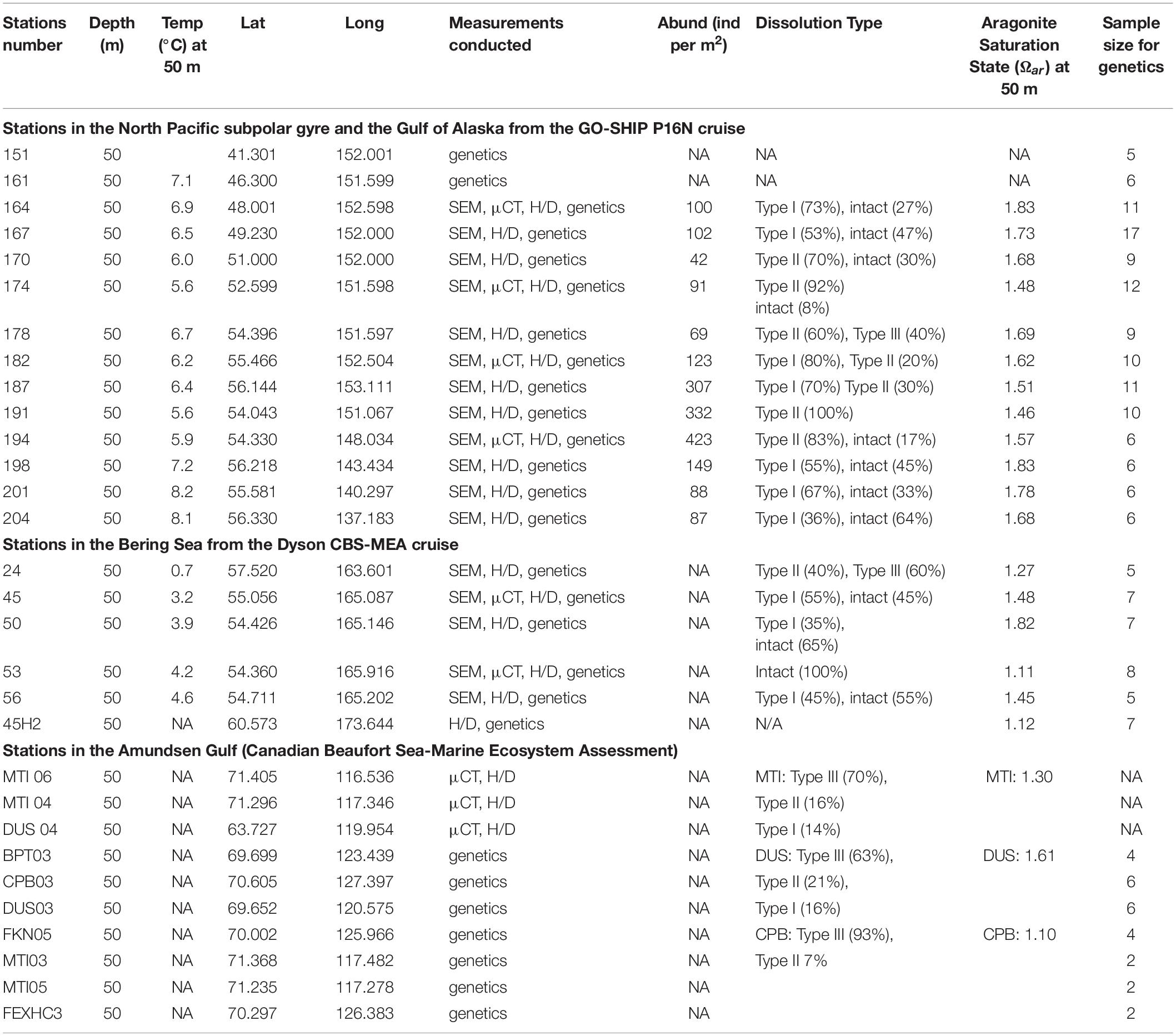
Table 1. Collected samples with indication for all the additionally conducted measurements on shell morphology, genetics, and dissolution estimates from the Eastern Pacific subpolar gyre and GoA on the GOSHIP P16N cruise; Dyson CBS-MEA in the Bering Sea cruise; and in the Amundsen Gulf.

Exposure to OA in the GoA Based on the GoA-COBALT Model

To estimate seasonal, decadal, and long-term exposure to OA in the GoA, we used model output from a hindcast simulation conducted with the GoA-COBALT (Carbon, Ocean Biogeochemistry and Lower Trophic) model (Hauri et al., 2020). This model is based on the three-dimensional physical Regional Oceanic Model System (ROMS, Shchepetkin and McWilliams, 2005), the modified version of the COBALT (3PS-COBALT, Stock et al., 2014; van Oostende et al., 2018) model, and the moderately high-resolution terrestrial hydrological model by Beamer et al. (2016). Physical initial and boundary conditions were taken from the Simple Ocean Data assimilation ocean/sea ice reanalysis 3.3.1 (SODA; Carton et al., 2018). Dissolved inorganic carbon (DIC) and total alkalinity (TA) initial conditions were taken from the mapped version 2 of the Global Ocean Data Analysis Project (GLODAPv2.2016b; Lauvset et al., 2016) data set. DIC was adjusted to the corresponding hindcast year using regional anthropogenic CO₂ estimates by Carter et al. (2017). Nitrate, phosphate, oxygen, and silicate initial conditions were extracted from the World Ocean Atlas 2013 (Garcia et al., 2013). All other variables were initialized based on a climatology from a GFDL-COBALT simulation (1988– 2007), as described in Stock et al. (2014). The model was run from 1980 to 2013 and was forced with atmospheric pCO₂ observations from the Mauna Loa CO₂ record (¹last accessed 22 January 2018). Winds, surface air temperature, pressure, humidity, and radiation were forced with data from the Japanese 55-year Reanalysis (JRA55-do) 1.3 project (Tsujino et al., 2018). Modeled freshwater was brought in from numerous rivers and tidewater glaciers at a 1 km resolution and daily timestep with point-source river input via exchange of mass, momentum, and tracers through the coastal wall at all depths (Beamer et al., 2016; Danielson et al., 2020). Nutrient, DIC, and TA concentrations in the freshwater were based on available observations (Stackpoole et al., 2016, 2017). The reader is referred to Hauri et al. (2020) for more information on the model and a detailed model evaluation.

Exposure to OA in the Bering Sea

Ocean acidification (OA) exposure in the Bering Sea was estimated with model results from a 10 km horizontal resolution implementation of the Regional Ocean Modeling System (ROMS; Shchepetkin and McWilliams, 2005; Danielson et al., 2011) denoted as “Bering10K”, coupled to the BEST-NPZ ecosystem model (Gibson and Spitz, 2011). Atmospheric forcing of air temperature, winds, specific humidity, rainfall, and shortwave and longwave radiation come from The Climate Forecast System Reanalysis (CFSR; Saha et al., 2010) and CVSv2 operational analysis (Saha et al., 2014). Tidal mixing and ice dynamics were also included. The BEST-NPZ ecosystem model recently underwent a substantial code revision aimed at improving model simulation of biological variables, namely primary productivity, through revisions to the ecosystem light and nutrient equations and by increasing the number of vertical layers from 10 to 30 (Kearney et al., 2020). This ecosystem model includes two phytoplankton groups (large and small), microzooplankton, large and small copepods, and euphausiids. Phytoplankton productivity consumes nutrients (nitrate, ammonium, iron) which are transferred to zooplankton biomass via grazing, or to detritus via mortality. Carbonate chemistry has also been added to model ocean acidity and elucidate underlying mechanisms of inorganic carbon cycling within different shelf regions (Pilcher et al., 2019). Boundary and initial conditions for DIC and TA were calculated from empirically derived fits with salinity using ship-based data collected during the Bering Sea Ecosystem Study (BEST) and Bering Sea Integrated Research Project (BSIERP). Freshwater runoff was modified to contain seasonally varying concentrations of DIC and TA representative of outflow from the mouth of the Yukon River. Atmospheric CO₂ varied seasonally following output from the NOAA Earth System Research Laboratory’s CarbonTracker 2016 Product (CT2016; Peters et al., 2007).

Estimating Spatial Connectivity Using Particle Tracking Model

To examine spatial connectivity in the GoA, we used hydrodynamic output from the model hindcasts described in Coyle et al. (2019). Atmospheric forcing of air temperature, winds, specific humidity, rainfall, and shortwave and longwave radiation were interpolated from the CFSR (Saha et al., 2010) and CVSv2 operational analysis (Saha et al., 2014). These hindcasts include coastal runoff (Beamer et al., 2016) as well as explicit tidal dynamics (and associated mixing). Tidally filtered weekly averaged velocities from this ROMS-based, 3-km resolution model were re-gridded to regular latitude-longitude-depth coordinates, and these values were subsequently interpolated to track particles forward in time, using a daily time step, at a constant 200 m depth.

The literature suggests that, due to prevalent currents, pteropods from the eastern North Pacific Gyre are advected (McGowan, 1963) into the GoA via northwards transport. As such, we initiated particle tracking in the offshore regions at 53°N in April for the following reasons: first, the prevalence of the northward advection that can carry pteropods from the offshore eastern Pacific subpolar gyre toward the GoA within the duration of their life cycle; second, the known offshore regional presence of pteropods and their spring spawning (e.g., Mackas and Galbraith, 2012; Doubleday and Hopcroft, 2015); third, southernmost boundary in the model domain where the initiation was feasible. The duration of particle tracking for 8 or 12 months was used to correspond to the pteropod life history, delineated by the completion of their early life stage into subadults or adults (Fabry, 1989). The particle tracking location with the shortest duration of initiation was thus used as an indicator of the early, most sensitive life stages, while the location of particles with the longest duration indicated the presence of the adults.

To examine spatial connectivity in the Bering Sea, a similar procedure was employed using output from the ROMS-based, 10-km resolution model described in Kearney et al. (2020). The physical structure and forcing of this model was identical to the version used for the Bering Sea OA exposure methods, as described above for the ROMS Bering 10K model. Regularly gridded, weekly averaged velocities from this model hindcast were interpolated to track particles backward in time using 60°N, 173°W as an ending location (on April 15, 2017) in a daily time step at a constant 50 m depth, which is an average depth distribution for L. helicina.

Morphometrics of Pteropod Morphotypes

Individuals of two different morphotypes of species Limacina helicina, recognized as L. helicina helicina and L. helicina pacifica, were selected from the samples to conduct the analyses at the morphotype level. The samples did not include morphotype characterization for individuals smaller than 0.5 mm in diameter. Individual pteropod height and width were measured with the Amscope software (Irvine, CA, United States) to subsequently determine specific morphotype. Separation of different morphotypes is possible only among the adults (McGowan, 1963; Janssen et al., 2019); thus, we only analyzed the adult life stages. Separation of the adults was first based on the presence or absence of striation (Janssen et al., 2019) and the shape of the shell (high spired shape vs flattened). The shape was reported as a height-diameter ratio (H/D) ratio (McGowan, 1963). Lower H/D ratios (flat shells) with no striation identified adult L. helicina pacifica, while higher H/D (with extended shell spire) and striation presence identified the adults of L. helicina helicina (Figure 2). When H/D ratios were plotted against the diameter of the shell, the shell proportions were fairly constant throughout the size range of the individuals collected, allowing subsequent separation of the two morphotypes (McGowan, 1963). Altogether, 98 individuals were analyzed for the morphometric analyses: 56 from the Eastern Pacific subpolar gyre, including the GoA, 17 from the Bering Sea, and 25 from the Amundsen Gulf. However, the sampling approach was not adequate to quantitatively determine spatial distribution of different morphotypes. We used both morphotypes for genetic analyses and shell dissolution analyses, while only L. helicina pacifica was used for investigating shell dissolution in combination with bulk shell density and thickness, due to insufficient sample numbers for L. helicina helicina.

FIGURE 2

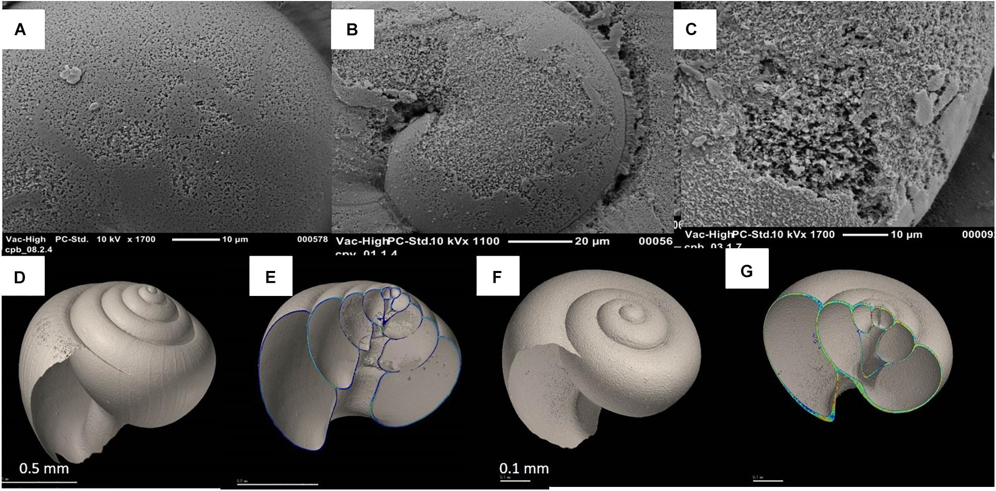
Figure 2. Various degrees of pteropod shell dissolution from the GoA and the Bering Sea, progressing from increased porosity, moderate to the most severe dissolution; Type I (A,B), Type II (B,C), and Type III (C). Two different Morphotypes of Limacina helicina: Limacina h. helicina (D) and Limacina h. pacifica (F) with respective images of their shell thickness for Limacina h. helicina (E) and for Limacina h. pacifica (G). Color bar indicates the CT number as a shell density from 380 (lowest density) to 1000 (highest density).

Bulk Shell Density and Thickness Using Microcomputer Tomography (μXCT)

For measures of pteropod shell deposition processes, an average of 10 organisms of L. helicina pacifica per station were analyzed for bulk shell density and thickness using micro-computed tomography (μXCT; Figure 2). Only the adult animals with greater than 4 whorls were analyzed, so that shell deposition patterns could be related to a single life stage, thus excluding the early life stages that could potentially introduce life-stage bias. We differentiated two morphotypes based on their H/D ratio (McGowan, 1963; Janssen et al., 2018), as well as the absence of striation. Therefore, density and thickness measurements were morphotype-specific (only on L. helicina pacifica). A total of 83 air-dried individuals were analyzed, 41 from the Eastern subpolar gyre with the GoA, 16 from the Bering Sea and 25 from the Amundsen Gulf. After overnight drying, a μXCT ScanXmate–D160TSS105 (Comscantecno Co., Ltd., Yokohama, Japan) was used to apply X-rays to the sample stage. This system can rotate through 360 degrees, with high-resolution settings (X-ray focus spot diameter, 0.8 μm; X-ray tube voltage, 80 kV; detector array size, 1024 × 1024; 1800 projections/360°, four-times averaging). This X-ray analysis focused on the aragonite shell; therefore, the soft tissue inside the shells was not considered and was numerically removed from the 3D images. Spatial resolution of the scanned image was from 1.0 to 1.2 μm, depending on the size of the shell. Reconstruction of 3D tomography was obtained by the convolution back projection (CBP) method used the ConeCTexpress (Comscantecno Co., Ltd., Yokohama, Japan). Calculation of shell thickness and density was performed by Molcer Plus imaging software (White Rabbit Corp., Inc., Tokyo, Japan).

To evaluate the bulk density of shell, we used the CT number. The CT number is a relative number of mean grayscale value with respect to the standard material of known density. When the object is constituted by a single substance, the CT number is proportional to the bulk density. In this study, we used a limestone grain (calcite crystal, calcite standard NIST RM8544 (NBS19)) with a 300 μm diameter as the standard material, which has the same composition of the target material. This limestone particle was used on individual pteropod shells for all analysis and the calculation of the CT number. Pteropod bulk shell density was evaluated by 16-bit grayscale contrasts (65,536 gray level gradations) of a transparent image achieved by μXCT. We used the CT number of the pteropod shell which is represented by equation 1:

$CTnumber=[(\mathrm{\mu }\mathrm{\_}shell-\mathrm{\mu }\mathrm{\_}air)/(\mathrm{\mu }\mathrm{\_}calciteSTD-\mathrm{\mu }\mathrm{\_}air)]\times 1000(1)$

where μ_shell, μ_air, and μ_calciteSTD were the X-ray attenuation coefficients of the sample, calcite, and air, respectively. The bulk shell density for an entire test was evaluated with equation 2:

$MeanCTnumber=\frac{1}{T}\sum _{n=230}^{1000}n{T}_n(2)$

where n was the CT number, T_n was the total number of voxels with a specific CT number (n), and T was the total number of voxels in the whole shell. The highest density was 1000 and the lowest density was 230, being represented by the boundary between the pteropod shell and the surrounding air. The mean CT number indicated the mean density of an individual test as normalized per shell length, which we refer to as ‘normalized shell thickness’ or ‘normalized bulk shell density’ in the text below.

Bulk shell density (g per cm^–3) was calculated from the mean CT number as following:

$Bulkshelldensity=(CTnumber-49.04)/350.47(3)$

Shell morphometrics (H/D ratio), thickness, and density data were compared with the observational data related to Ω_ar to investigate the impact of carbonate chemistry on shell-building processes over the depth of the water column inhabited by the pteropods (sensu Bednaršek et al., 2014). In addition, shell density and thickness were statistically correlated to the H/D ratio across all the investigated basins using either linear or polynomial regression (Supplementary Figure 1).

Shell Dissolution

We identified the incidence of different types of shell dissolution across individuals (Table 1 and Supplementary Figure 2) collected along carbonate chemistry gradients and compared shell dissolution across different regions of the subpolar gyre, GoA and Bering Sea. While evaluating shell dissolution, it is important to have as unbiased process as possible. Thus, while we randomly selected the individuals for shell dissolution not to introduce any bias in the shell examination process, we also made sure we had a sufficient number of organisms present to determine any difference in the shell dissolution between two different morphotypes. When the number of organisms allowed for this, we aimed to equally split the analyzed subsample between two different morphotypes (in the North Pacific subpolar gyre and the GoA); however, when this was not possible due to insufficient amount of pteropod individuals (such as in the Bering Sea), then we analyzed whatever morphotypes were present. The occurrence of pteropod shell dissolution in the Amundsen Gulf, as relevant to this study, has been described by Niemi et al. (2021) and here only discussed briefly. Shell dissolution was assessed for each individual and an average value was calculated per station (Table 1 and Supplementary Figure 2). We analyzed 10-15 individuals from each of 12 stations from the subpolar gyre, including the GoA, and 6 stations from the Bering Sea.

We prepared each individual by removing the organic layer using a combination of protocols (Bednaršek et al., 2012b, 2016a). Briefly, pteropods were transferred from 100% to 70% and 50% ethanol in gradual steps, rinsed thoroughly with DI water, exposed to diluted bleach (5% sodium hypochlorite) for a treatment of approximately 30 min that was subsequently rinsed with DI water for 2-3 times to clean the shell surface, and subsequent air-dried for 12 h. Mounted samples were coated with a combination of Au-Pd for 120 s at 35A before being examined under the scanning electron microscopy (SEM).

For measures of shell dissolution severity, the presence of three categories of dissolution was assessed following Bednaršek et al. (2012b). Type I indicated a shallow, upper-prismatic level of dissolution, followed by Type II with modest dissolution protruding deeper into the cross-lamella layer, and Type III indicating the most severe dissolution protruding deeper into the crystalline layers (Supplementary Figure 2). The percentage dissolution type occurrence was assessed per each individual and correlated with the observational cruise data related to Ω_ar in the subpolar gyre, the GoA and the Bering Sea.

Genetic-Based Analyses

Sample Collection

Between five and 17 individuals per station were sampled from the Bering Sea and Gulf of Alaska cruises (Table 1). Sampling was opportunistic and depended on frequency and condition of individuals collected at each station. An additional 13 individuals were sampled from the Amundsen Gulf to act as “outlier” samples to determine species or subspecies distribution across broader oceanographic basins (Table 1). Individuals were photographed prior to DNA extraction and their morphotypes were recorded using the methods described above.

DNA Extraction, PCR, and Sequencing

DNA from each individual was extracted using the QIAGEN DNeasy tissue extraction kit (Hilden, Germany). An approximately 600 base pair region of Cytochrome c oxidase I (COI) unit was amplified using universal primers for marine invertebrates (Forward: GGTCAACAAATCATAAAGATATTGG, Reverse: TAAACTTCAGGGTGACCAAAAAATCA; Folmer et al., 1994; Geller et al., 2013; Sromek et al., 2015b). Polymerase chain reactions comprised 10–15 ng of template DNA, 4.0 mM MgCl₂ and GoTaq G2 Master Mix (Promega, United States), using an initial cycle at 98°C for 3 min, 30 cycles of 10 s at 98°C, 30 s at 55°C and 30 s at 72°C, and 5 min at 72°C. PCR products were Sanger sequenced in both directions at a commercial facility (Molecular Cloning Laboratories, San Francisco, CA, United States). Consensus haplotype sequences for each individual were created using the COI forward and reverse sequences obtained.

To determine whether there was evidence for cryptic species within the regions we sampled, we examined genetic distances between individual haplotypes and visualized the data using phylogenetic trees. The haplotype distribution across the two morphotypes was explicitly examined. To determine whether there was evidence for population structure, genetic distances were calculated within and between haplotypes at each geographic station. Finally, the sequences generated as part of the current study were compared to previously published sequences (Supplementary Tables 1, 2), to determine whether there was any evidence for species or population differentiation across the range of L. helicina.

In all analyses, sequences were aligned between individuals using the Muscle algorithm (Edgar, 2004). Pairwise distances (p-distance) between haplotypes and populations were estimated in MEGA V7.0 (Kumar et al., 2016), and standard error estimates were derived using 500 bootstrap replicates (Supplementary Tables 3, 4). Phylogenies between haplotypes were determined using a Minimum-spanning network (Bandelt et al., 1999), calculated in PopART (Leigh and Bryant, 2015).

Results

Habitats of Concern in the Subpolar Gyre and GoA as Related to OA

The P16N cruise data (from 2015) in the subpolar gyre and GoA shows that the dissolution-inducive corrosive waters (threshold for severe dissolution Ω_ar < 1.2; Bednaršek et al., 2019) are shallowest at about 53°N, 152°W (Figure 3), with the isolines of Ω_ar < 1.2 deepening both to the south in the southern subpolar region and to the north on the GoA continental shelf. The corrosive waters are characterized by “low” temperature (< 6°C), high DIC (> 2180 μmol kg−1), and Ω_ar < 1.2 (Figures 3A–F).

FIGURE 3

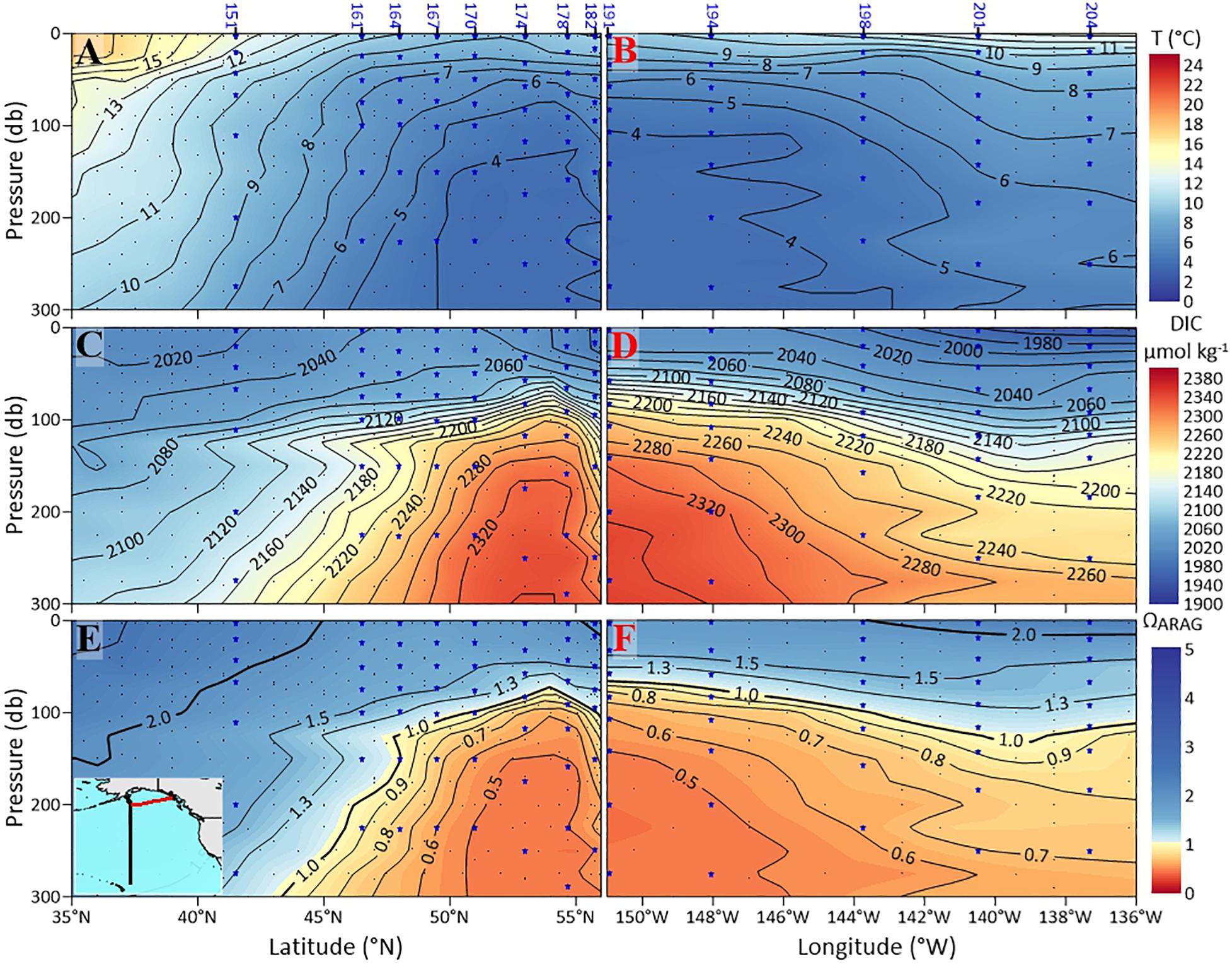
Figure 3. Plots of observational data from the P16N cruise (Eastern Pacific subpolar gyre and the GoA) sections of: potential temperature °C (A,B); dissolved inorganic carbon (DIC) in μmol kg^–1 (C,D); and aragonite saturation state, Ω_ar (E,F). The sections on the left are from the south to north transect (black-colored contour on the small map), and the sections on the right (red colored contour on the small map) are from the west to east transect (see insert map in E). The pteropod station numbers are at the top. Indicated are the two solid black contour lines showing Ω_ar of 1 and 1.3.

GoA-COBALT model output (Hauri et al., 2020) of the time series of Ω_ar at 54°N, 152°W and at 57°N, 152°W indicate that the Ω_ar shoaling into the upper 50 – 100 m of the water column occurs during winter and early spring, partially extending into summer (Figure 4). At depths greater than 100 m, most of the deeper waters across the GoA and shelf region are undersaturated with respect to aragonite (Ω_ar < 1). In the GoA model outputs from 2013, there is a west-to-east deepening of Ω_ar in the upper 100 m of the water column, with the minimum Ω_ar occurring at about 51-55°N, 152°W, in the subpolar gyre (Figures 3, 5). Accordingly, the depth of the Ω_ar saturation horizon (where Ω_ar = 1) is shallowest in the western part of the study region (< 100 m) and deepens toward the eastern side of the subpolar gyre to approximately 110-130 m (Figure 6). The highest saturation state and deepest aragonite saturation horizon occur in the summer and autumn months, and significantly lower saturation states and shallower Ω_ar horizon occur during winter and early spring months (Figure 4). Summertime subsurface Ω_ar (spatially averaged across 50 to 100 m depth, and temporally averaged across June, July, and August) is generally < 1.3 across the region, especially in the near-shore regions of the northern and eastern GoA. From Kodiak (57°N/150°W) southward, wintertime (temporally averaged across December, January, and February) subsurface Ω_ar increases to levels > 1.3 along the shelf, while off the shelf, a large area stays undersaturated with respect to Ω_ar (Figure 4A). In the central region of the subpolar gyre and the GoA, Ω_ar saturation horizon is located near 50 m throughout the year (Figure 5A), while seasonal changes in the Ω_ar saturation horizon in the eastern part of the GoA cause shorter periods of exposure to low Ω_ar conditions (Figures 5A,B).

FIGURE 4

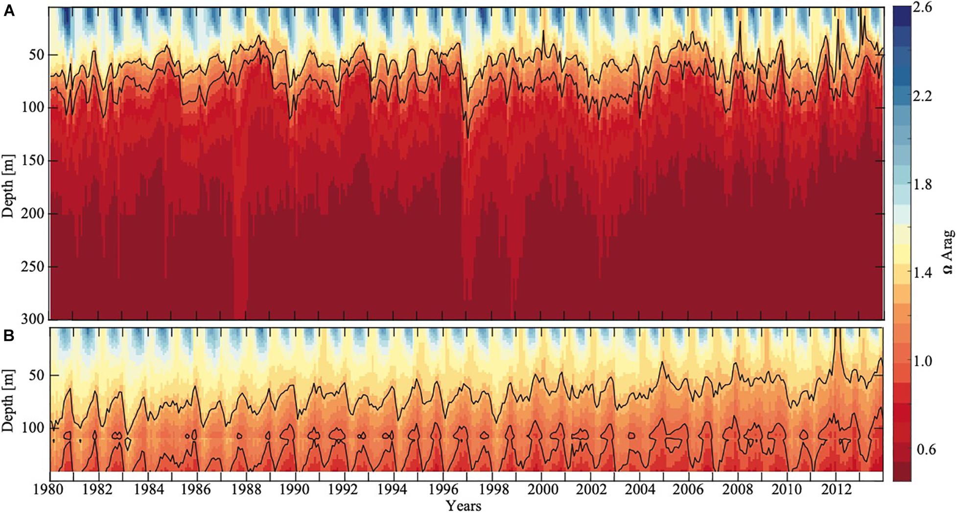
Figure 4. Modeled aragonite saturation state of the Eastern Pacific subpolar gyre and the GoA as a function of depth and time (years) at station 191 (A, 54°N and 152°W) and at a random location on the shelf (B, 57°N and 152°W). Solid black contour lines show Ω_ar equal to 1 and 1.3. On the shelf, the seafloor is located at around 140 m depth (white area). Model output is from the GoA -COBALT hindcast simulation described by Hauri et al. (2020).

FIGURE 5

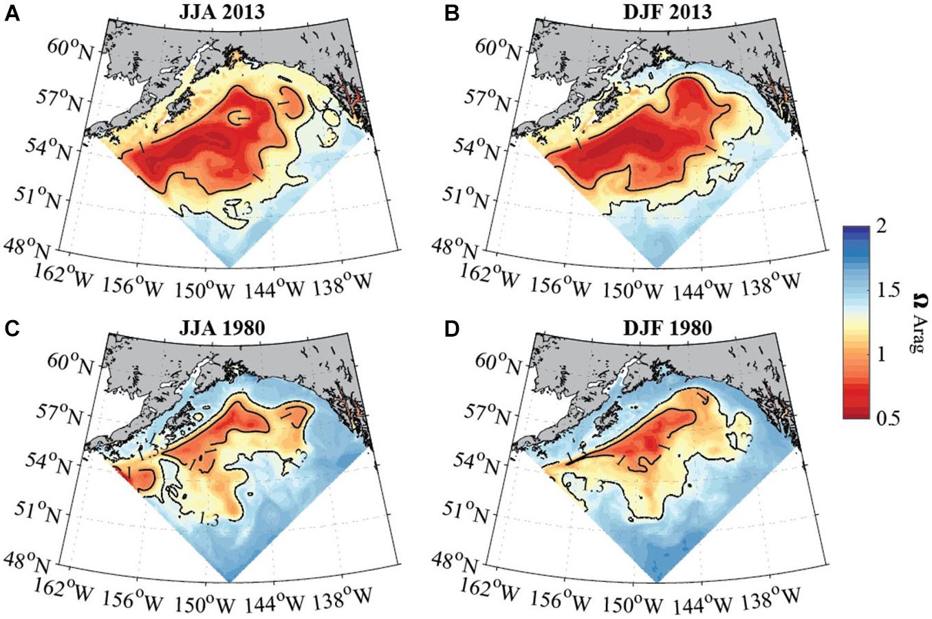
Figure 5. Average seasonal aragonite saturation state (modeled data) across the upper 50 to 100 m in the GoA for June to August (A,C; left column) and December to February (B,D; right column) for 2013 (top row) and 1980 (bottom row). Solid black contour lines depict aragonite saturation state equal to 1 and 1.3. White areas show locations where the topography is shallower than 50 m. Model output is from the GOA-COBALT hindcast simulation described by Hauri et al. (2020).

FIGURE 6

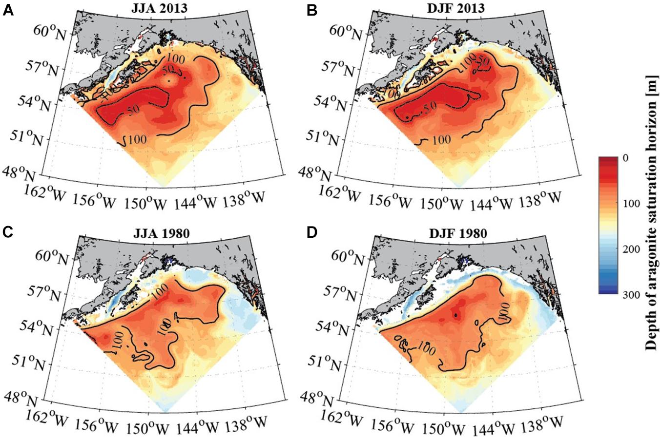
Figure 6. Average seasonal depth of the aragonite saturation horizon [m] in the GoA for June to August (A,C; left column) and December to February (B,D; right column) for 2013 (top row) and 1980 (bottom row). Solid black contour lines depict depth of the aragonite saturation horizon at 50 and 100 m (modeled data). White areas show locations where the aragonite saturation (Ω_ar) horizon is deeper than the topography, indicating the absence of undersaturated waters. Model output is from the GOA-COBALT hindcast simulation described by Hauri et al. (2020).

Decadal Changes in OA Habitats in the GoA Over the 34-Year Period

In evaluating long-term change in the subpolar gyre and GoA since the 1980s, the model output suggests significant decline of Ω_ar in the upper 100 m of the water column (Figure 4). The area of undersaturated water over the 50 to 100 m depth range more than doubled between 1980 and 2013 at the location of the model output (Figure 4A). Such modelling results are consistent with large-scale field observations (Carter et al., 2017). While some subsurface waters are already undersaturated with respect to aragonite in 1980, areas of Ω_ar < 1 are now much more widespread across the GoA. Furthermore, in 1980, Ω_ar frequently reach levels < 1.2 in waters deeper than 50 m, while in more recent years, Ω_ar also frequently reaches levels < 1.2 in the upper 50 m of the water column in both on- and off-shelf areas on a seasonal basis (Figure 6). In particular, the subpolar gyre is significantly lower in Ω_ar in the winter months. While Ω_ar conditions in the subpolar gyre in the 1980s ranged from 0.8 < Ω_ar < 1.2, current ranges are from 0.5 < Ω_ar < 0.8. Overall, the center of the subpolar gyre is currently the most vulnerable to the effects of increasing OA (Hauri et al., 2021). Although the eastern part of the GoA has seen a similar magnitude of change, the current OA conditions are less severe.

Current Habitats of Concern With Respect to OA in the Bering Sea

The Bering Sea 10K model output suggests that in the subsurface water between 50 and 100 m Ω_ar is < 1.3 across nearly all of the Bering Sea shelf, and Ω_ar < 1 for large portions of the northwestern shelf for both winter (December-February) and summer (June-August) months (Figure 7). In Figure 7, regions with a depth < 50 m, which are representative of the inner-shelf domain, are excluded. Subsurface Ω_ar values are generally lower in summer months compared to winter months, except for a relatively small region of buffered waters within Bristol Bay. The most corrosive waters are located in the northwestern Bering Sea. Panels A and B in Figure 8 illustrate a depth profile of model output for Ω_ar along the midnorth (MN) shelf transect (denoted by the magenta line in Figure 7). Phytoplankton productivity in surface waters and respiration at depth generate a very strong vertical gradient in Ω_ar during summer, compared to a relatively weak vertical gradient in winter. Surface Ω_ar values are greater than 2 during the summer, but less than 1.3 during the winter. Panel C in Figure 8 shows the modeled vertical profile of Ω_ar at an outer shelf location over the entire 2003–2012 period. This figure illustrates the seasonal cycle of low winter surface values, followed by higher surface Ω_ar values in spring-summer, and a subsequent subsurface drawdown in autumn due to respiration. Such intense seasonal changes in the spatial and vertical Ω_ar conditions define the exposure time of less favorable conditions (Ω_ar < 1.3) on a seasonal basis. The subsurface values of Ω_ar tend to decrease by ∼0.1 over the 2003-2012 timeframe, coinciding with a shift in physical variability from a warm temperature period to a cold temperature period. This temperature shift in the colder years due to increased vertical mixing and nutrient resupply in the euphotic layer (Pilcher et al., 2019) generates an increase in primary productivity and anthropogenic carbon uptake, with subsequent increase in respiration that exacerbates the expected OA trend over this timeframe. The surface trends of 0.025–0.04 units/year are significant for the inner and middle shelf domains (Pilcher et al., 2019).

FIGURE 7

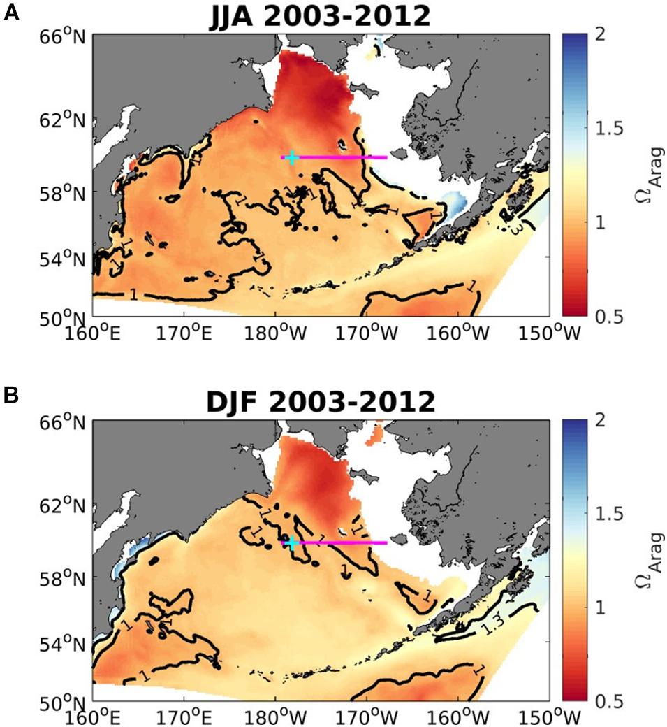
Figure 7. Average seasonal aragonite saturation state (Ω_ar) across the upper 50 to 100 m in the Bering Sea for June to August (A; upper) and December to February (B; lower), averaged over 2003-2012 (modeled data). Solid black contour lines depict aragonite saturation state equals 1 and 1.3. White areas show locations shallower than 50 m. Magenta line shows the midnorth (MN) shelf transect, and cyan plus-sign denotes the MN18 station location. Model output is from the Bering10K hindcast simulation described by Pilcher et al. (2019).

FIGURE 8

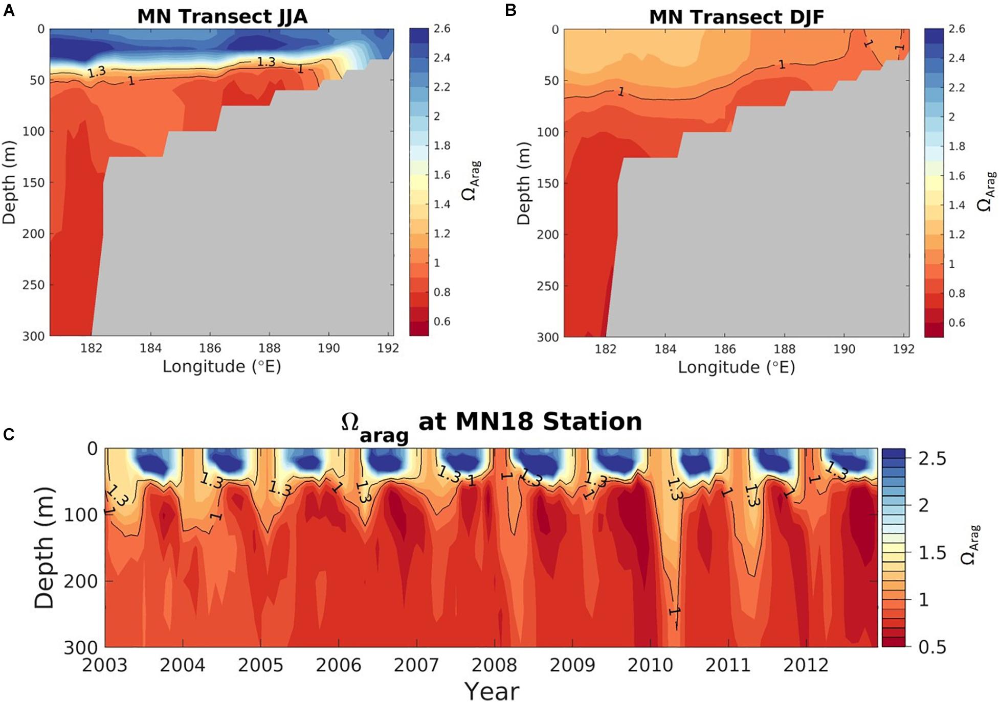
Figure 8. Transect plots of aragonite saturation state (Ω_ar) in the Bering Sea, along the midnorth (MN) shelf transect line, denoted by the magenta line in Figure 7, for (A) June July August (JJA) and (B) December, January, February (DJF), averaged over 2003-2012 (modeled data). (C) Aragonite saturation state at station MN18 (cyan plus-sign, Figure 7) as a function of depth (y-axis), and time (x-axis). Model output is from the Bering10K hindcast simulation described by Pilcher et al. (2019).

Current Conditions in the Amundsen Gulf

Generally, in the Canadian sector of the Amundsen Sea, the supersaturated conditions occurred in surface waters, while undersaturated conditions (Ω_ar < 1) occurred across the Gulf in the Pacific halocline layer (50–200 m). Some smaller-scale variation in the Ω_ar is possible, depending on the transects sampled (Figures 9A–C), with such conditions described in more detail by Niemi et al. (2021). In the areas where pteropods were collected, Ω_ar in the Pacific layer ranged from 0.76 to 1.3, and averaged around 0.88, indicating that the pteropods’ main habitat is largely corrosive in summer (Figure 9).

FIGURE 9

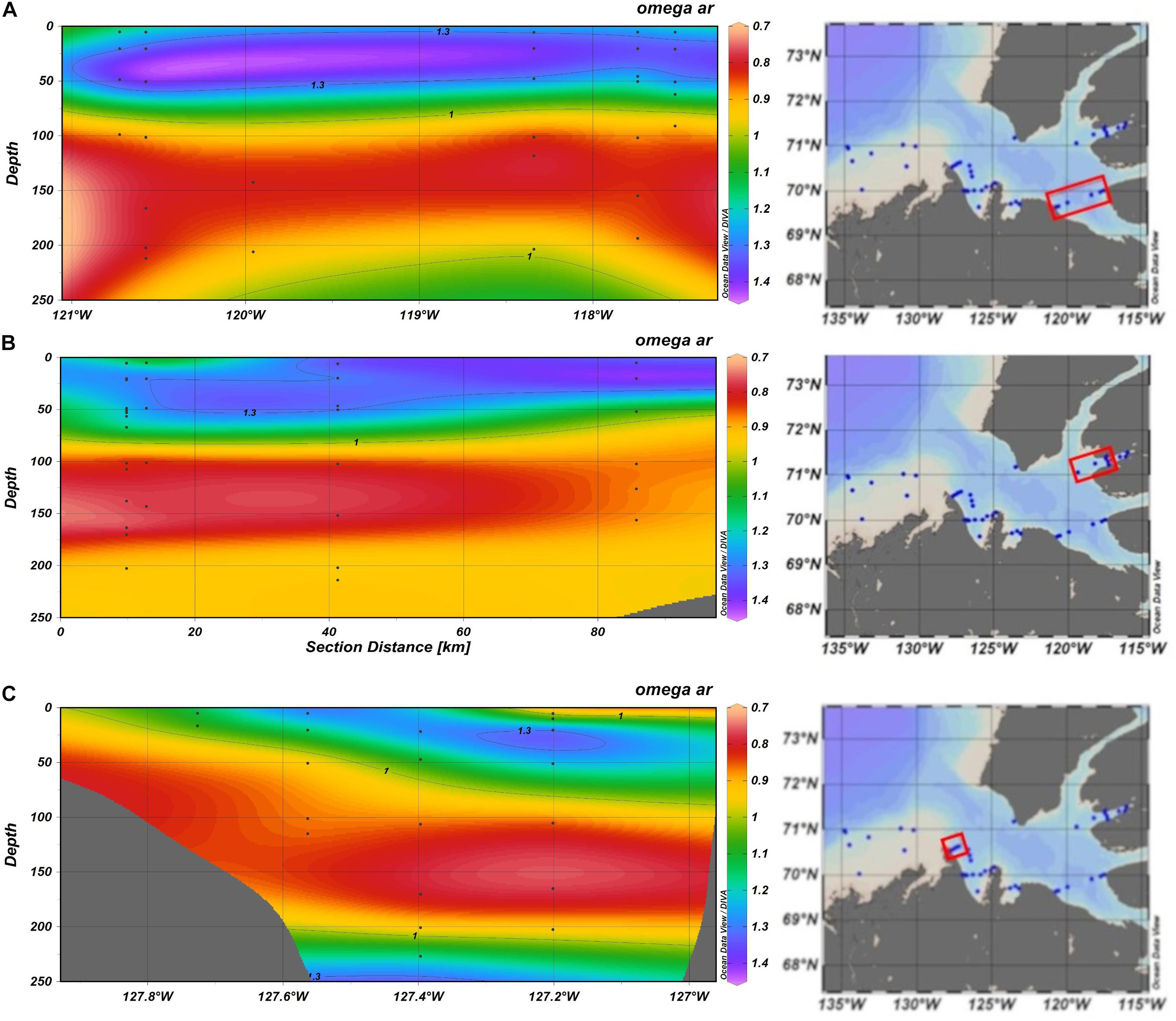
Figure 9. Transect plots of aragonite saturation state (Ω_ar; based on the observational data) in the Amundsen Gulf in the Canadian Arctic sampled in August 2018. Transects extend across Dolphin and Union Strait (A); Minto Inlet (B) and across the mouth of the Gulf from Cape Bathurst (C). Red boxes on the transect maps include the biological stations investigated for pteropod shell dissolution (previously published in Niemi et al., 2021).

Sensitivity-Related Biological Parameters

Morphotype Distribution

Pteropods were present across all of our study regions in high abundances, especially from 55 °N (Table 1). Based on the presence of striations, as well as H/D ratios, two adult morphotypes were detected: L. helicina helicina with an inflated spire and striated whorls (Figure 2D), and L. helicina pacifica with a depressed flat spire and no striation (Figure 2F). The H/D ratios plotted against the diameter of the shell showed a relatively constant ratio, regardless of the size range of the adults (Supplementary Figure 1A). The ranges of H/D values for the two morphotypes were similar to those previously reported by McGowan (1963). The H/D range for L. h. pacifica was between 0.8 to 1, while H/D range for L. h. helicina was higher than 1. All morphotypes were found in all three basins (Supplementary Figure 1B).

Shell Thickness and Density Related to the Shell Morphometrics

The distribution of H/D ratios in two morphotypes was also related to a specific range of normalized shell thickness and density (Supplementary Figures 1C,D). Normalized bulk shell thickness showed an inverted bell curve shape relationship with the H/D ratio; its decrease was correlated with declining H/D ratios to a value of approximately 0.9 to 1. Below this ratio, normalized shell thickness started to increase (polynomial fit with R² = 0.17, p-value = 8.622E-05). These results indicate that the organisms with lower spire (lower H/D range) built thicker shells compared to those on the upper range that built thinner shells (Supplementary Figure 1C). The density was not dependent on the H/D ratio, with similar densities across the range (R² = 0.052; p = 0.0155; Supplementary Figure 1D).

Environmental Control on Shell Building Processes

The impact of Ω_ar on the processes of pteropod morphometrics and shell characteristics (H/D ratio, normalized bulk shell density and thickness) across all investigated ocean regions (GoA, Bering, Amundsen) was examined in one morphotype, L. h. pacifica only. The H/D ratio of adult individuals was significantly correlated with Ω_ar. Linear regressions showed the best fit of H/D ratio to be correlated with the Ω_ar, at 50 m (Ω_ar,50) representing an average depth of daily pteropod vertical migration (Figure 10A; R² = 0.6966, p = 8.074E-16). Linking shell morphometrics with the Ω_ar, adult individuals with higher H/D ratios (extended shell with higher spire) were observed at higher Ω_ar, while the organisms with lower H/D (flatter shell with lower spire) were present at lower Ω_ar. We fitted normalized bulk shell thickness against Ω_ar averaged over 100m depth (Ω_ar,avg100). The best linear fit shows the shell thickness to significantly increase with a declining Ω_ar,avg100 (Figure 10B; R² = 0.31, p-value = 0.028). At higher values of Ω_ar, adult pteropods built shells with higher H/D ratios and lower shell thicknesses (Figures 10A,B; Supplementary Figure 1). We also fitted shell thickness against the Ω_ar at 100 m; the best fit found was polynomial one, where shell thickness increased up to a Ω_ar of 1.1, upon which it started to decrease (R² = 0.623; p-value = 2.581E-07; Figure 10C). This value could be considered an inflection point (threshold), below which the shell building processes start to decline. Such patterns were observable when combining the data of L. helicina pacifica across investigated ocean regions. However, on the regional basis, the lack of sufficient data or limited Ω_ar,avg100 condition gradients prevented us from making conclusions for each region separately, especially for the Bering Sea region with its narrow range of Ω_ar,avg100 conditions. Normalized bulk shell density was not significantly correlated with Ω_ar,avg100 (R² = 0.027, p-value = 0.273; Figure 10D). These results imply that only the processes influencing shell thickness, and not density, were impacted by the carbonate chemistry conditions.

FIGURE 10

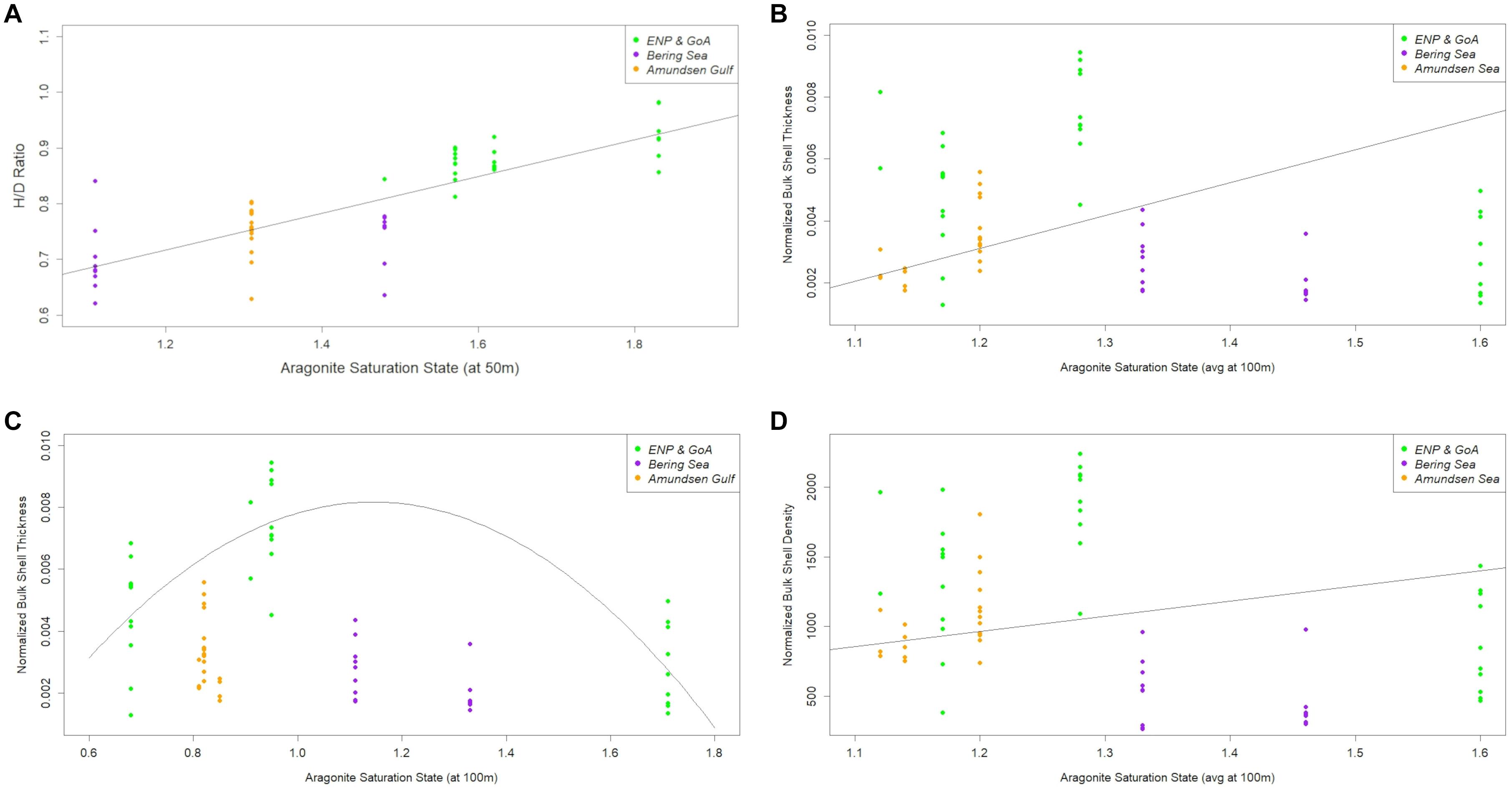
Figure 10. Height-diameter (H/D) ratio distribution (A), normalized bulk shell thickness with linear fit (B), normalized bulk shell thickness with polynomial fit (C), and normalized bulk shell density (D) along the omega saturation state (ar) in three basins (based on the observational data) in Limacina helicina pacifica. The equations for correlation with omega saturation state (Ω_ar) or the combination of temperature and Ω_ar are following: Shell morphology (H/D; Figure 10A) = 0.32095+0.33014* Ω_ar; Normalized Shell Thickness (linear; Figure 10B) = 0.001459+0.001895* Ω_ar; Normalized Shell Thickness (polynomial, Figure 10C) = 0.005569−0.0010466* Ω_ar −0.0004721* Ω${}_{ar}^2$; Normalized Shell Thickness (f (T and Ω_ar)) = 6.803*10⁻³−3.984*10⁻⁵*T-2.364*10⁻³* Ω_ar; Normalized Shell Density (Figure 10D) = −182.5+294.3* T −234.9* Ω_ar.

Pteropod Shell Dissolution Across the Regions

High resolution observations of pteropod shell surface under SEM demonstrated a range of dissolution values, depending on observed Ω_ar conditions at the specific sample locations (Figure 2). The samples collected during spring-summer in the subpolar gyre and the GoA were characterized by a notable difference in the shell dissolution, with the stations across the central and western side of the study region (stations 178-191, Figure 11) showing the greatest severity of dissolution (Table 1). The areas of dissolution spatially coincide with the regions characterized by a shallower Ω_ar depth horizon, depicted in both the observational data and model outputs (Figure 5). In comparison, shell dissolution declined toward the east, with complete disappearance of any dissolution patterns east of 139°W. In addition, the more inshore locations (Station 187) had less severe dissolution compared to the offshore samples. This result again coincides with the GoA-COBALT model output of higher Ω_ar onshore and lower Ω_ar and shallower Ω_ar saturation horizon offshore (Figures 5, 11).

FIGURE 11

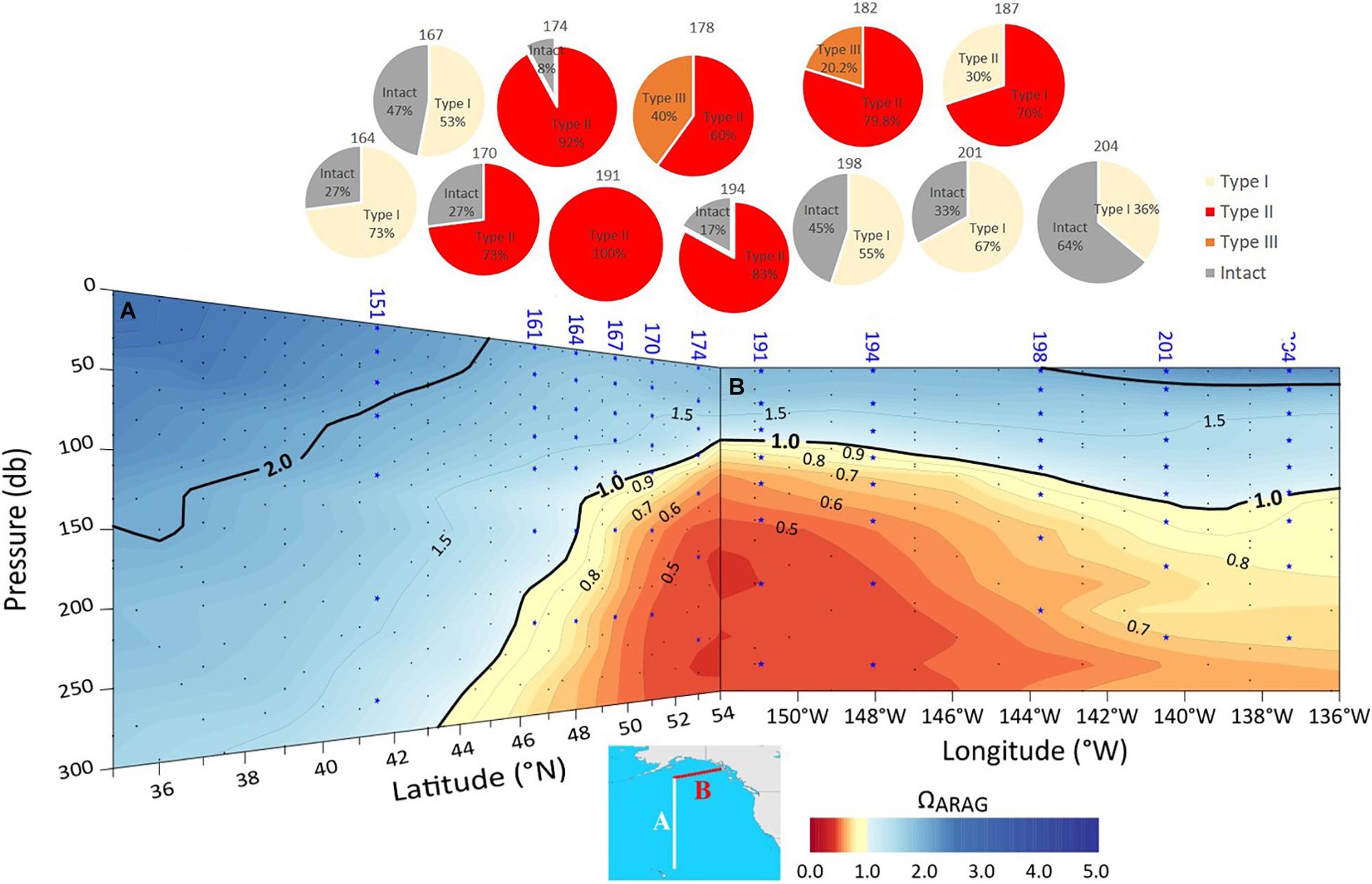
Figure 11. The depth of the aragonite saturation state (Ω_ar; based on observational data) along two sections conducted on P16N cruise in the Eastern P16N cruise in the Eastern Pacific subpolar gyre (A) and GoA (B). with corresponding proportions of different types of pteropod shell dissolution. Pteropod samples were analyzed from stations 164 to 204.

Out of the six collected samples in the Bering Sea during spring-summer, various dissolution ranges were observable (Table 1), mostly characterized by Type I and II dissolution, with only station 24 having more severe (Type III) dissolution present. Because there was insufficient data from the cruise to interpolate across the stations, we could not correlate shell dissolution with the oceanographic gradients as in the GoA, so we used the model output instead (Figures 7, 8). The stations with the most severe dissolution were distributed over the central part of the eastern Bering Sea shelf. This coincides with the model outputs of the observed shallow Ω_ar horizon and Ω_ar < 1 around 50 m depth during this period, which is also in the Bering 10k model output. Intact organisms were present in the southern part of the Bering Sea and around the Aleutian Islands, with the Ω_ar horizon positioned at depth ranges below 100 m.

Shell dissolution in the Amundsen Gulf was described in detail by Niemi et al. (2021). In short, shell dissolution was widespread, occurring at coastal and offshore locations as well as in small embayments. In an initial assessment of 134 samples of L. helicina, greater than 85% of individuals exhibited severe dissolution. The majority of shell damage occurred on the first whorl, indicating that damage likely occurred in early life stages during the spring period (May/June) when sea ice may still be present in the Amundsen Gulf. Overall, we found no observable difference in shell dissolution between two different morphotypes across any of the high latitude regions, indicating that shell dissolution is not a trait that would be morphotype-specific.

Biological Parameters Related to Resilience and Adaptive Capacity

Genetic Analyses

A total of 176 individuals were sequenced at cytochrome c oxidase I (COI) across 21 stations (Supplementary Tables 1, 2). Of these, 130 represented the L. helicina helicina phenotype and 38 represented the L. helicina pacifica phenotype. The phenotype of eight sequences were not determined due to sample deterioration. After alignment, 544bp were shared across all individuals, representing 20 unique COI haplotypes across the entire dataset.

Haplotype diversity was low (Supplementary Table 3): overall nucleotide diversity was 0.005 (SE 0.001). Pairwise distances between individual haplotypes varied between 0.002 and 0.009. These values were lower than accepted for species definition at the CO1 locus (Hebert et al., 2003). The samples were dominated by three haplotypes (Figure 12A): Haplotype 1 was found in 118 individuals, Haplotype 2 in 34 individuals, and Haplotype 3 in 5 individuals. The remaining haplotypes were found in two individuals (Haplotype 4 and 5) or in one individual only (Haplotypes 6-20).

FIGURE 12

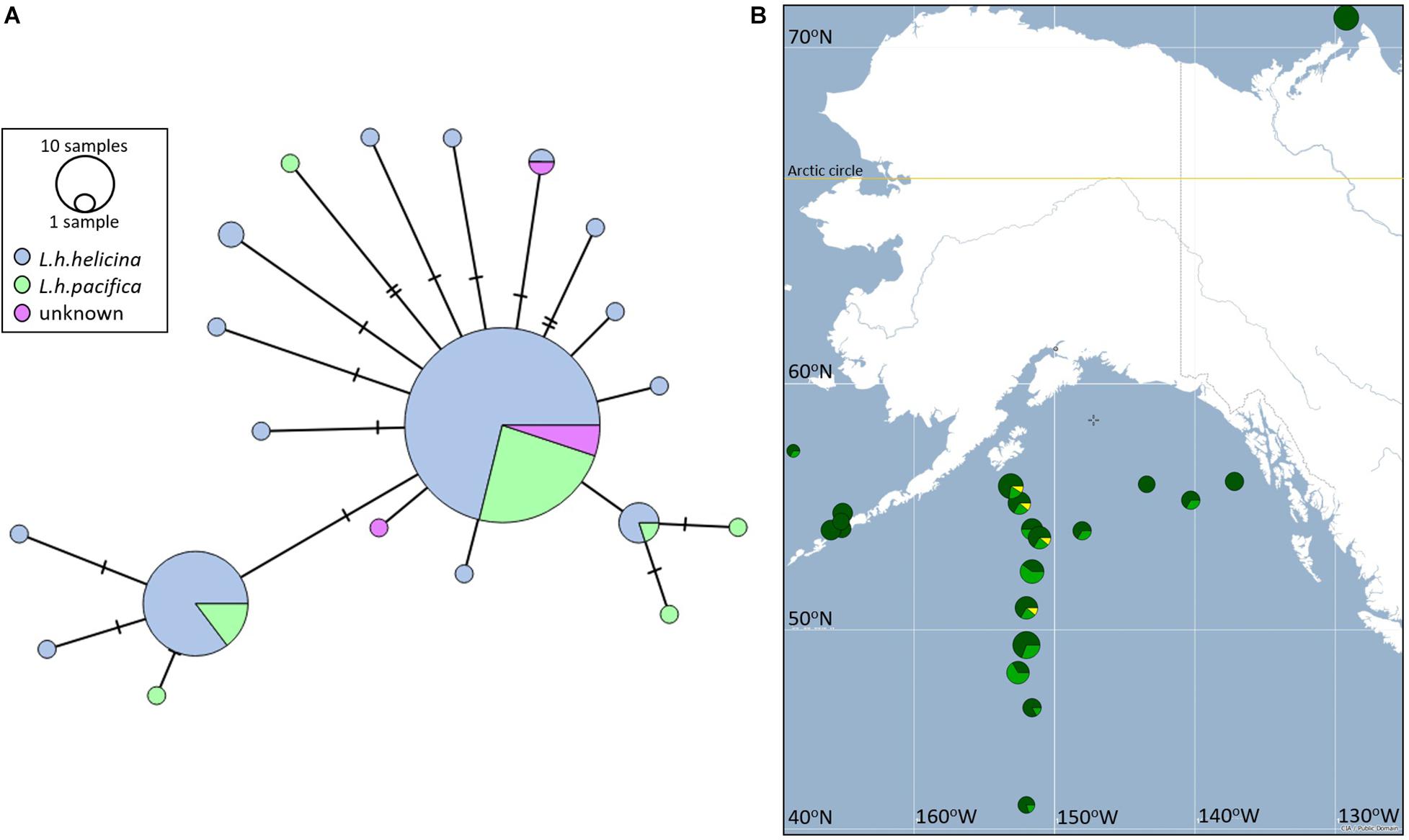
Figure 12. (A) Minimum spanning network between 20 CO1 Haplotypes sequenced across 176 L. helicina morphotypes, sampled from the eastern North Pacific, GoA, Bering Sea and Amundsen Gulf. Haplotypes are joined by number of mutations (horizontal lines), circle sizes represent number of individuals representing each haplotype. The two morphotypes are represented in blue (L.helicina helicina) and green (L. helicina pacifica). Samples in purple could not be phenotyped. (B) Distribution of the three most common COI haplotypes across sampling stations in the Eastern Pacific subpolar gyre, GoA, Bering Sea and the Amundsen Gulf.

The minimum spanning network described a star phylogeny for CO1 haplotypes (Figure 12A); that is, several short branches connected by a common haplotype. Such phylogenies are often interpreted to represent an evolutionarily recent founder event, followed by population expansion. There was no evidence for genetic differentiation between L. helicina morphotypes (Figure 12A). Both morphotypes were represented within three most frequent haplotypes.

Visualization of the frequency distributions of the three most common haplotypes (1-3) suggests that sequence diversity decreases in the northernmost populations, particularly in the Bering Sea and Amundsen Gulf (Figure 12B). However, formal analysis of haplotype diversity between stations sampled revealed no significant differences between populations (Supplementary Table 4). Divergence of haplotype frequencies between populations varied between 0.001 and 0.002, with standard errors falling in the same order of magnitude. The power of this analysis may be affected by sample sizes, which varied between 5 and 17 individuals per station. However, given the high frequency of the most common haplotype, as well as the close relationship between these haplotypes, large sample sizes per station would be required to detect putative differences.

A total of 259 published COI sequences (Supplementary Table 2) were combined with the 179 sequences derived from this study and were grouped into nine broad geographic regions: Amundsen Gulf, Bering Sea, subpolar gyre, Greenland, Kara Sea, Hudson Bay (Northern Canada), Western North Pacific, Svalbard and White Sea. Global haplotype divergence was small, with most haplotypes differing from each other by a few mutations (Supplementary Figure 3). However, two previously described haplogroups (Abyzova et al., 2018; Shimizu et al., 2018) described the data, with evidence of a unique haplogroup limited to Svalbard and the Kara Sea, and dominance of the second haplogroup in the Bering Sea, Amundsen Gulf and North Pacific Seas. While the haplogroups differ by only a few mutations, these data suggests separate colonization and divergence events and broad-scale population structure. However, pairwise tests for divergence (Supplementary Table 5) revealed small pairwise distances between geographic regions.

Spatial Connectivity Based on Particle Tracking Model Outputs

Particle tracking models were used to investigate pteropod spatial connectivity over the subpolar gyre in the GoA. These were based on the assumption of a northward juvenile pteropod advection from the eastern North Pacific and life duration of approximately eight months to a year, during which pteropods would reach adulthood. The results indicate that pteropods were dispersed throughout the entire area during this period, irrespective of location origin (Figure 13), with high abundances present (Table 1). On the other hand, shorter durations of particle tracking indicated the locations of the early life stages, which are dependent on the location of their spawning.

FIGURE 13

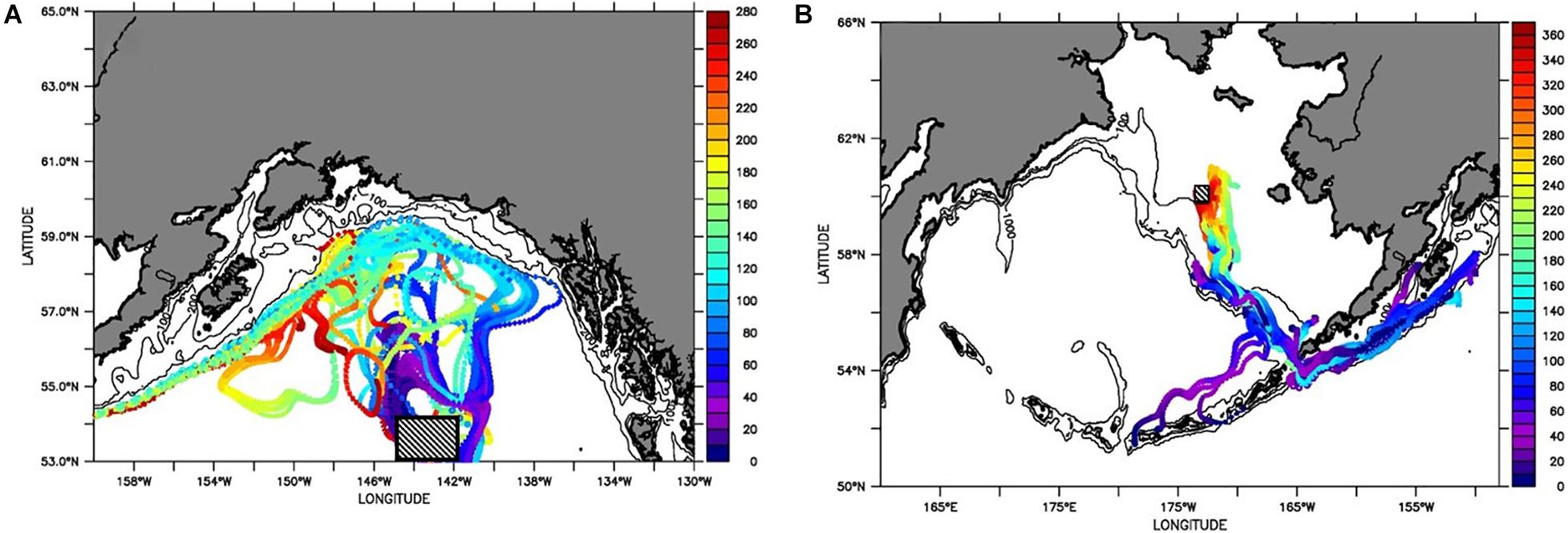
Figure 13. Particle tracking at (A) 200 m depth in the Eastern Pacific subpolar gyre for a time period of 8 months (280 days), and (B) at 50 m depth in the Bering Sea for the time period of 12 months (365 days). Vertical scale bar indicates (A) number of days in the forward tracked particles since their release near 53°N, 143°W on April 15, 2012; and for (B) days of the backward tracked particles using 60°N, 173°W as ending location on April 15, 2017 (with initial release in April 15, 2016). Blue colors indicate shorter, and red color indicate longer time intervals since release. Initial release is indicted by a square. The hydrodynamic output from the model hindcasts is described by Coyle et al. (2019) and Kearney et al. (2020).

Northward advection dominates in the first three months after the typical spawning period in late spring. In the following 4–8 months, flow of the GoA waters occurs westward along the Aleutian Islands (Figure 13A). If initiation is assumed to occur in the offshore subpolar gyre, the early life stages can thus reach the GoA in the summer, while the subadults and adults would be distributed in the GoA’s coastal and shelf region and advected westward in the winter. The dispersal of the particles over long distances demonstrates large-scale biogeographic distribution with no apparent species boundaries across the entire area.

Extensive spatial connectivity was also observed in the Bering Sea (Figure 13B), where we tracked particles backward in time for a full year from a mid-shelf location on the northwestern shelf. This ending location was chosen based on observational results. Particles reaching this destination all originated from the south, primarily from the Gulf of Alaska (passing through Unimak Pass), but also from the deep basin to the north of the Western Aleutian Islands. From either starting location the particles travel along the shelf break to the north of the Aleutian Islands during an approximately 8-month period, subsequent to their initial release in April. In general a smaller spread of particles was observed for the Bering Sea than was the case in the GOA. Note these results are not strictly comparable, as we tracked particles forward in time in the GOA case, and backwards in the Bering Sea case. It is further possible that more dispersion would have been obtained with a different ending location in the Bering Sea. Fundamentally, however, the smaller spread of the Bering Sea tracks reflects the presence of vigorous 200-km scale eddies in the deep GOA, as compared to the relatively quiescent conditions on the shallow Bering Sea shelf.

Discussion

This interdisciplinary study provides an integrated OA risk assessment for high-latitudinal pteropod populations of the subpolar gyre, GoA, Bering Sea and Amundsen Gulf. Here, we synthetize multi-faceted components of the risk assessment, as defined by OA exposure, species and morphotype sensitivity, and resilience through genetic structure and spatial connectivity.

Model output comparisons between the two regions (the GoA and the Bering Sea) revealed the differences in the magnitude of Ω_ar conditions, both in the context of the vertical gradients and seasonal cycles related to Ω_ar. Overall, the model outputs as well as data based on P16N cruise observations (Figure 1), suggest that Ω_ar is lower in the North Pacific subpolar gyre, while the habitats in the eastern part of the GoA seem to be less OA-compressed, providing more favorable conditions for pteropod populations. The Bering Sea, in comparison, has somewhat lower values of Ω_ar and a shallower Ω_ar horizon than the subpolar gyre/GoA. This observation is consistent with decreasing Ω_ar towards the poles in North-Pacific-Arctic waters (Mathis et al., 2015), indicating that this region may have experienced more severe biological impacts corresponding with the changes, especially in the last two to three decades (Carter et al., 2017). Seasonality is an important parameter to consider, because it defines the duration of exposure to less favorable conditions. In the GoA, the subsurface conditions are less favorable in the summer, while the subsurface conditions in the Bering Sea are less favorable in the winter (Figures 5–8). As illustrated by the Bering Sea model, vertical habitat suitability is reduced in the summertime, showing persistent subsurface Ω_ar < 1.2 conditions despite high surface Ω_ar conditions that are buffered by substantial primary productivity. There is a clear exception in the subpolar gyre, where unfavorable conditions appear to persist throughout the year. Still, while surface waters of the subarctic Pacific are projected to become Ω_ar < 1 (Bindoff et al., 2019), global model simulations suggest that surface waters of the Bering Sea will remain supersaturated even under the RCP 8.5 scenario. Hence, the upper surface waters represent suitable habitat for sensitive pelagic calcifiers. However, it remains uncertain if the vertical migrators, such as pteropods, could only occupy surface waters given their ecological dependence on deeper depths (Lalli and Gilmer, 1989).

With respect to the trend observed over the last 34 years, the GoA-COBALT model output of the subpolar gyre and the GoA suggests a declining trend of Ω_ar and shoaling of the Ω_ar saturation horizon. This indicates that pteropod populations have been experiencing an increase in exposure to lower Ω_ar in their habitats over decadal time scales. While we do not have biological data over the same time period as the model output, we assume that it is very likely that the severity of pteropod shell dissolution described here is a consequence of rapid, multiple human-related impacts in the region, and not a natural change in the region (Mathis et al., 2015; Carter et al., 2017; Hauri et al., 2021). The lack of a hindcast simulation in the Bering Sea does not allow such biological risk assessment over a longer time period.

Insights into the seasonal carbonate chemistry variability is important to infer the impacts of exposure within the L. helicina life history. The life cycle of northern high-latitude pteropods is regionally specific, lasting between 1 and 2 years (Kobayashi, 1974; Fabry, 1989; Gannefors et al., 2005), and is characterized by late spring-summer spawning, with subsequent presence of subadults and adults during the winter periods of the corresponding years. Successful recruitment depends mostly on survivorship during two key periods: the early life stages that have higher sensitivity to OA, and the adult stages that are responsible for successful spawning and recruitment (Bednaršek et al., 2016b). Model outputs during the spring-summer period can be used to characterize exposure of the early life stages (larval and juveniles) to OA, while the model outputs integrated over the upper 50–100 m of the water column for the winter months can serve as an approximation of the adult exposure (Bednaršek et al., 2019). The summer conditions in the GoA are more favorable, thus early life stages will be less impacted relative to the adults that experience lower Ω_ar wintertime exposure. In contrast, the Bering Sea has opposite seasonality, characterized by the summer reduction of the suitable Ω_ar conditions, with adults being less impacted compared to the early life stages. It is also important to note that regionally specific conditions, like the year-round unfavorable conditions in the subpolar gyre, might impact both early and adult life stages, delineating this region of the highest OA concern.

Observations of adult pteropod shell dissolution during spring-summer surveys in both basins spatially correlate with the spring spatial carbonate chemistry patterns, as delineated by the P16N cruise observations and biogeochemical models in the GoA and subpolar gyre (Figures 1, 11). In the GoA, there was more severe dissolution in the western part of the study area, coinciding with the highest pteropod abundances, and less severe dissolution in the onshore waters. In the Bering Sea, severe dissolution occurred in the north-central part, where the model outputs projected lower Ω_ar compared to the higher Ω_ar in the south. The GoA is more likely to experience severe spring and summertime dissolution of pteropod shells compared to the same period in the Bering Sea. Our data show that thinner shells, along with dissolution uniformly distributed around the shell surface, are evidence of an impact related to lower Ω_ar cumulative exposure (Bednaršek et al., 2016a). This is opposite to the conclusion from Peck et al. (2016); namely that dissolution only occurs if the periostracum is damaged or if imposed through predation pressure. More severe dissolution in the Amundsen Gulf likely occurs because of the dominance of undersaturated Pacific waters within the pteropod habitat, where prolonged low Ω_ar exposure could represent higher risks, characteristic of the polar habitats of the Northern Hemisphere. Given that our genetic analyses show that the Amundsen Gulf pteropods share the same species distribution as the GoA and the Bering Sea individuals, there is no reason to believe that another more resilient species or subspecies will replace the current populations (Niemi et al., 2021).

There are additional parameters that can impact shell processes (Bednaršek et al., 2018; Oakes and Sessa, 2020), including regional parameters that can reverse the shell patterns observed in this study (Mekkes et al., 2021), making it important to compare the differences always among the same morphotypes. Seasonal patterns of high primary production in the Bering Sea could potentially offset some of the negative effects (sensu Bednaršek et al., 2018), with temperature and oxygen also playing a role in the shell building processes (Mekkes et al., 2021). Both the GoA and the Bering Sea pteropods have substantially less severe dissolution compared to that reported in the Arctic regions, such as the Amundsen Gulf. Limited extent of shell repair in the form of crystalline regrowth was reported in the presence of abundant food availability only in a few adult organisms (Niemi et al., 2021). Against a general pattern of thinner shells with only a few individuals displaying limited shell repair, this data shows high risk for pteropod population. Our findings therefore do not support the observation of pteropod resilience to OA by Peck et al. (2018).

Sensitivity and adaptation capacity were evaluated by examining the shell morphometric characteristics. Flatter and thicker (lower H/D) individuals were found in habitats associated with more severe Ω_ar, while high-spire, less thick (high H/D) individuals were present at higher Ω_ar. This distribution likely indicates that pteropods can build thicker shells and display some plastic responses, thus indicating a phenotypic response in the less favorable conditions that protects them against intense shell dissolution. A divergent range of plastic responses in the two distinct phenotypic morphotypes could be differential acclimation to Ω_ar exposure. The extended height over the same diameter results in higher surface shell area of L. helicina helicina, pointing towards the fact that a larger extent of shell surface can be exposed to the surrounding waters compared to L. helicina pacifica with lower surface area. As such, we postulate that different morphotypes might develop in the native habitats characterized by the intensity of Ω_ar exposure. By inhabiting more intense OA conditions, L. helicina pacifica may form flatter and thicker shells to protect the shell against more severe exposure to lower Ω_ar. Flatter shells with lower surface exposure is intended to reduce the exposure to low Ω_ar, while thicker shells can potentially tolerate more extensive dissolution better at lower Ω_ar. On the other hand, L. helicina helicina inhabits the habitat with less severe, low Ω_ar exposure and does not need such protecting mechanisms; greater shell surface and thinner shells can be sustained at less intense OA condition.

Pteropod morphotype distribution data over much larger spatial scales in the North Pacific clearly demonstrates the eastward occurrence of L. helicina pacifica, while L. helicina helicina is dominant westwards (McGowan, 1963). In combination with the carbonate chemistry data over the examined area that shows a progressing shoaling of carbonate chemistry eastwards (Carter et al., 2017; Cai et al., 2020), there is a spatial pattern of L. helicina helicina inhabiting the westward region with higher Ω_ar and L. helicina pacifica present in the lower Ω_ar eastward region, to which they seem to be more adapted to via their morphometric characteristics. However, given the presences of both morphotypes across the stations of the investigated area of the subpolar gyre and the GoA, our study is likely not spatially extensive enough to be able to demonstrate differential morphotype occurrence over Ω_ar scales.

In terms of shell building processes, pteropods continue building their shells even under lower Ω_ar conditions (sensu Comeau et al., 2010) but at reduced growth rates, presumably due to the trade-offs in the compensatory processes. However, it seems that the conditions of around 1.1 < Ω_ar > 1.3 (Figures 10B,C) could be delineated as a threshold below which the shell building process becomes energetically more expensive, and thus, shell processes start to decline. A similar Ω_ar biomineralization threshold was previously reported by Bednaršek et al. (2019). Interestingly, shell density seems to be an independent process not driven by Ω_ar, likely pointing towards the fact that building a shell with consistent density is an important process for the organisms and is thus more tightly regulated than processes governing shell thickness. While the differences across the eastern-western area in aragonite saturation state were substantially different, we note minimal differences in temperature across the same area, with only 1-2°C difference (Figures 3A,B), suggesting a relatively homogenous habitat temperature wise (sensu McGowan, 1963). As Ω_ar and temperature are highly colinear in both basins, it makes it impossible to differentiate which parameter is a major driver behind the biological responses. In addition, the lack of data on other potentially important parameters, such as food availability (sensu Bednaršek et al., 2018) is currently not allowing for a more accurate interpretation and prediction of the drivers and mechanisms behind the biomineralization processes and population-level outcomes under future OA intensification.

Beside a direct impact of OA on reproduction (sensu Manno et al., 2016), there could be indirect implications of energetic expenditure related to reproductive outputs. The assumption is that higher Ω_ar conditions would allow individuals to potentially invest more energy into growth, resulting in larger shells with greater tissue mass. Building shells under low Ω_ar conditions (below 1.1) would require greater energetic investment, which may be indirectly reflected in smaller-sized organisms. Since the reproductive efforts of the individuals are inherently linked to tissue weight (Lalli and Gilmer, 1989), smaller-sized organisms with lower gamete production might have a lower reproductive effort under future OA intensification.

Examining the parameters related to the adaptation capacity (genetic structure, cryptic species, and spatial connectivity) is also important to potentially determine the morphotype-level risks on pteropod population level. For example, OA-induced exposure would not necessarily result in local vulnerability if individuals were replaceable or if spatial connectivity may bring new flux of organism from less impacted areas, while the presence of genetically differentiated subspecies with differential response to OA might buffer changes in distribution and abundance. Despite morphological differences, genetic analyses reveal that there was no basis for differentiation between these two forms at the species level, because both share mitochondrial DNA haplotypes. In addition, particle tracking modeling indicates that the organisms are well mixed over the investigated area, supporting genetic uniformity of the investigated pteropods. Therefore, we suggest that the differences in morphotypes might reflect phenotypic plasticity related to the differential exposure to prevailing OA-related environmental conditions, but likely not limited to Ω_ar only. Alternatively, such differences may arise through fine- scale population structure and local adaptation; this explanation cannot be ascertained with our available data. We conclude that there is no evidence for cryptic species or subspecies across the geographic ranges sampled, based on tests for divergence at the mitochondrial DNA cytochrome oxidase I locus. It is unlikely that hidden species diversity may account for differential morphotype responses to low Ω_ar. It is possible that there is within-species diversity that should be examined using nuclear DNA markers. Our results reveal a possible reduction in haplotype diversity in northern populations, which may point toward population differentiation. However, this result was not significant. On a species-wide range, the previously reported differentiation between unique haplogroups in the Arctic Ocean north of mainland Europe (Kara Sea and Svalbard), the Western North Pacific (Shimizu et al., 2018), and the Okhotsk Sea (Shimizu et al., 2021) was supported here by the addition of further samples from the subpolar gyre, the Bering Sea, and Amundsen Gulf. While the differences between the two haplogroups were small, the results suggest population structure at the species-wide scale, explained by separate colonization events with subsequent divergence over broad geographic ranges. These results are intriguing, given that the single molecular marker used has relatively little power to differentiate between populations.

Investigations based on particle analyses and prevailing advective patterns suggest extensive spatial connectivity. These analyses further support the result of a single cosmopolitan species of L. helicina, revealed by the mitochondrial DNA analyses. Given the time trajectories of the particles modeled here, the results suggest a continuous process of repopulation and intermixing of pteropods in the GoA region in the spatial context of the North Pacific subpolar gyre. High connectivity might alleviate localized negative impacts, especially if different morphotypes are constantly repopulating this region, therefore providing resilience. However, poor survival at different life history stages may affect recruitment throughout the region. For example, the early life stages encounter exposure to low Ω_ar conditions between 53 and 56°N through northward advection. It is also unknown to what degree adaptive capacity at the population level may buffer recruitment variation. Overall, high risk for pteropod population persistence with intensification of OA has to be assumed because of their known vulnerability, along with low evidence for species diversity and the progressive severity of OA exposure, despite their wide connectivity across the considered habitats and our insufficient knowledge on their adaptive capacity in the high latitudes.

Corresponding with pteropod high risk related to OA in the high latitudinal habitats are also high-risk repercussion for the commercially important fisheries and high trophic levels marine vertebrates. Considering the magnitude of OA change in this region coupled with a high pteropod biomass (Bednaršek et al., 2012a; Doubleday and Hopcroft, 2015), negative pteropod population implications could ultimately have an impact for the fisheries dependent on pteropods as a food source, most explicitly for the various salmon species, cod and char, during the fall time in the absence of the other food sources essential for successful fish development. Moreover, given the changes in pteropod shell building processes, i.e. reduced calcification and shell thickness and lower H/D ratio, along with increased dissolution, these high latitudinal regions’ with one of the highest pteropod abundances on a global scale (Table 1; Bednaršek et al., 2012a) might also experience potentially significant biogeochemical effects related to the biological pump, resulting in the lower carbonate export fluxes over time (Carter et al., 2021; Lee and Feely, 2021; Sulpis et al., 2021). The results of this study suggest that an important component of the alkalinity change in the North Pacific may be the result of changes in pteropod production and dissolution. Moving forward into the future, the ecological and biogeochemical implications of these long-term changes will depend on multiple interacting processes, including the morphotype distribution, net shell calcification and dissolution, changes in the morphometrics, their abundance and phenology.

Given the dominance of pteropods in the subpolar gyre and the GoA, long-term observations should be strategically positioned along the W-E gradients where the differences in OA are most pronounced. Understanding of biological vulnerability on the regional scales provides an opportunity to prioritize monitoring to manage, and thus potentially reduce, the realized impact on the fisheries and ecosystems in the high-latitudinal ecosystems under predicted climate change scenarios.

Data Availability Statement

All sequence data are available in Genbank under accession numbers MZ502688–MZ502863 and in the Supplementary Material. The GoA-COBALT model output is publicly available (https://doi.org/10.24431/rw1k43t, Hauri et al., 2020). Carbonate chemistry data from the hydrographic cruise P16N are archived in the NCEI database: https://www.ncei.noaa.gov/data/oceans/ncei/ocads/metadata/0163182.html. The carbonate chemistry data from the Amundsen Gulf (2018) are publicly available in the Ocean Carbon Data System (OCADS), NCEI Accession number 0238161 (https://www.ncei.noaa.gov/data/oceans/ncei/ocads/metadata/0238161.html). The Bering10K model output fields and particle tracking output for the Bering Sea and Gulf of Alaska used in this analysis are available online from the Zenodo library (https://doi.org/10.5281/zenodo.5117852). Model source code for the Bering10K ROMS model is available here (https://github.com/beringnpz/roms-bering-sea). Pteropod abundance data from the GoA and the Bering regions are archived in the NCEI database, along with the hydrographic P16N data; data from the Amundsen Gulf are currently available upon request (Niemi) and will be submitted into the NCEI after the manuscript acceptance. Pteropod shell dissolution data and shell morphometrics and properties are available upon request (Niemi, Bednaršek; pers. communications), followed by the submission into the NCEI database after the manuscript acceptance.

Author Contributions

NB wrote the manuscript with contributions from all coauthors. NB and K-AN conceived the research, analyzed the data, and provided visualizations. CH, DP, and AH provided model outputs. NB directed the zooplankton fieldwork. AN provided biological data from the Amundsen Gulf. RF and CM provided carbonate chemistry data. KK analyzed pteropod shell density and thickness and contributed to the findings about the relevance of environmental data. All authors contributed to the article and approved the submitted version.

Funding

This work was funded by the North Pacific Research Board (NPRB; project number 1615: Pteropods as indicators in the high latitudinal environment) awarded to NB and K-AN. CH acknowledges funding from the National Science Foundation (NSF; Grant Nos. OCE-1459834 and 1656070). RF acknowledges support from the NOAA GOMO Program.

Conflict of Interest

The authors declare that the research was conducted in the absence of any commercial or financial relationships that could be construed as a potential conflict of interest.

Publisher’s Note

All claims expressed in this article are solely those of the authors and do not necessarily represent those of their affiliated organizations, or those of the publisher, the editors and the reviewers. Any product that may be evaluated in this article, or claim that may be made by its manufacturer, is not guaranteed or endorsed by the publisher.

Acknowledgments

We thank Isadora Jimenez-Hidalgo for her technical expertise and Lorenz Hauser and Ana Ramón-Laca for their advice in genetic analyses. We also thank AFSC team, Phyllis Stabeno and Janet Duffy-Anderson. We are grateful to Colleen Harpold and Nissa Ferm to conduct pteropod sampling in the Bering Sea, as well as Peter Proctor for collecting samples for carbonate chemistry in the Bering Sea, and to Shaun Bell to help assist analyses of physical-chemical parameters from Bering Sea cruises. Carbonate chemistry analyses in Beaufort shelf was done in the lab of Kumiko Azetsu-Scott at BIO, funded by ACCASP. Special thank you goes to Jesse Turner who collected pteropod samples on P16, Brendan Carter to collect carbonate chemistry samples, also to Alison MacDonald for making pteropod sampling on P16 feasible. We also thank S. Punshon and J. Charette for carbonate chemistry sample and data analysis for the Amundsen Gulf. We are grateful Arie Janssen with help on distinguishing different pteropod morphotypes.

Supplementary Material

The Supplementary Material for this article can be found online at: https://www.frontiersin.org/articles/10.3389/fmars.2021.671497/full#supplementary-material

Supplementary Figure 1 | The distribution of two different morphotypes based on the H/D ratios (L. helicina helicina and L. helicina pacifica) (A), and as separated per different ocean basins (B). The H/D ratio was correlated with the normalized shell thickness (C) and the density (D) from the individuals across the three ocean basins.

Supplementary Figure 2 | Depiction of three different types of dissolution (each column representing Type I, II or Type III) found on the pteropod shells collected across different basins (gyre, GoA, Bering, and Amundsen Gulf). Types and the extent of dissolution are linked with the sample location and additional analyses conducted on the samples (Table 1). Each photo depicts the type of shell dissolution of the individual organism from a different sampled location, with the scale bar indicating the size.

Supplementary Figure 3 | Minimum spanning network between CO1 Haplotypes sequenced across 427 individual L. helicina, sampled from the Amundsen Gulf (abbr. BeauSea), Bering Sea (abbr. BerngSea), Eastern North Pacific (abbr. ENPac), Greenland (abbr. Grnld), Kara Sea (abbr. Kara), Hudson Bay (abbr. NCanada), Western North Pacific (abbr. WNPac), Svalbard (abbr. Svbd) and White Sea. Haplotypes are joined by number of mutations (horizontal lines), circle sizes represent number of individuals representing each haplotype.

Supplementary Table 1 | COI gene sequences for both morphotypes of L. helicina across all the investigated regions (subpolar gyre, GoA, Bering, Bering Sea, Amundsen Gulf).

Supplementary Table 2 | Referenced studies, locations, and accession numbers of the previously published COI gene sequences for Limacina helicina.

Supplementary Table 3 | Estimates of Evolutionary Divergence (p-distance) between COI haplotype sequences 1-20 (in bold), genotyped in L. helicina collected from the North Pacific, Bering Sea and Amundsen Gulf. Below the diagonal: number of base pair differences per site calculated between haplotypes. Standard error estimate(s) derived from 500 bootstrap replicates are above the diagonal.

Supplementary Table 4 | Estimates of Evolutionary Divergence (p-distance) between Stations, based on COI haplotype sequences sampled at each station. The number of base differences per site from averaging over all sequence pairs between groups below the diagonal, standard error estimate(s) derived from 500 bootstrap replicates are above the diagonal.

Supplementary Table 5 | Estimates of Evolutionary Divergence (p-distance) between regions. The number of base differences per site from averaging over all sequence pairs between groups below the diagonal, standard error estimate(s) derived from 500 bootstrap replicates are above the diagonal. The samples originate from the North Pacific (abbr. ENPac), Greenland (abbr. Grnld), Kara Sea (abbr. Kara), Hudson Bay (abbr. NCanada), Western North Pacific (abbr. WNPac), Svalbard (abbr. Svbd) and White Sea.

Footnotes

1. ^ https://www.esrl.noaa.gov/gmd/ccgg/trends/data.html

References

Abyzova, G. A., Nikitin, M. A., Popova, O. V., and Pasternak, A. F. (2018). Genetic population structure of the pelagic mollusk Limacina helicina in the Kara Sea. PeerJ 6:e5709.

Google Scholar

Armstrong, J. L., Boldt, J. L., Cross, A. D., Moss, J. H., Davis, N. D., Myers, K. W., et al. (2005). Distribution, size, and interannual, seasonal and diel food habits of northern Gulf of Alaska juvenile pink salmon, Oncorhynchus gorbuscha. Deep Sea Res. Part II 52, 247–265. doi: 10.1016/j.dsr2.2004.09.019

CrossRef Full Text | Google Scholar

Auburn, M. E., and Ignell, S. E. (2000). Food habits of juvenile salmon in the Gulf of Alaska July–August 1996. N. Pac. Anadr. Fish. Comm. Bull. 2, 89–97.

Google Scholar

Bandelt, H. J., Forster, P., and Röhl, A. (1999). Median-joining networks for inferring intraspecific phylogenies. Mol. Biol. Evol. 16, 37–48.

Google Scholar

Beamer, J. P., Hill, D. F., Arendt, A., and Liston, G. E. (2016). High-resolution modeling of coastal freshwater discharge and glacier mass balance in the Gulf of Alaska watershed. Water Resour. Res. 52, 3888–3909. doi: 10.1002/2015wr018457

CrossRef Full Text | Google Scholar

Beauchamp, D. A., Cross, A. D., Armstrong, J. L., Myers, K. W., Moss, J. H., Boldt, J. L., et al. (2007). Bioenergetic responses by Pacific salmon to climate and ecosystem variation. N. Pac. Anadr. Fish. Comm. Bull. 4, 257–269.

Google Scholar

Bednaršek, N., Možina, J., Vogt, M., O’Brien, C., and Tarling, G. A. (2012a). The global distribution of pteropods and their contribution to carbonate and carbon biomass in the modern ocean. Earth Syst. Sci. Data 4, 167–186. doi: 10.5194/essd-4-167-2012

CrossRef Full Text | Google Scholar

Bednaršek, N., Tarling, G. A., Bakker, D. C., Fielding, S., Cohen, A., Kuzirian, A., et al. (2012b). Description and quantification of pteropod shell dissolution: a sensitive bioindicator of ocean acidification. Glob. Chang. Biol. 18, 2378–2388. doi: 10.1111/j.1365-2486.2012.02668.x

CrossRef Full Text | Google Scholar

Bednaršek, N., Johnson, J., and Feely, R. A. (2016a). Comment on Peck et al: vulnerability of pteropod (Limacina helicina) to ocean acidification: shell dissolution occurs despite an intact organic layer. DSRII 127, 53–56. doi: 10.1016/j.dsr2.2016.03.006

CrossRef Full Text | Google Scholar

Bednaršek, N., Feely, R. A., Reum, J. C. P., Peterson, B., Menkel, J., Alin, S. R., et al. (2014). Limacina helicina shell dissolution as an indicator of declining habitat suitability owing to ocean acidification in the California Current Ecosystem. Proc. R. Soc. B Biol. Sci. 281:20140123. doi: 10.1098/rspb.2014.0123

PubMed Abstract | CrossRef Full Text | Google Scholar

Bednaršek, N., Harvey, C. J., Kaplan, I. C., Feely, R. A., and Možina, J. (2016b). Pteropods on the edge: cumulative effects of ocean acidification, warming, and deoxygenation. Prog. Oceanogr. 145, 1–24. doi: 10.1016/j.pocean.2016.04.002

CrossRef Full Text | Google Scholar

Bednaršek, N., Feely, R. A., Tolimieri, N., Hermann, A. J., Siedlecki, S. A., Waldbusser, G. G., et al. (2017). Exposure history determines pteropod vulnerability to ocean acidification along the US West Coast. Sci. Rep. 7:4526. doi: 10.1038/s41598-017-03934-z

PubMed Abstract | CrossRef Full Text | Google Scholar

Bednaršek, N., Feely, R. A., Beck, M. W., Glippa, O., Kanerva, M., and Engström-Öst, J. (2018). El Niño-related thermal stress coupled with upwelling-related ocean acidification negatively impacts cellular to population-level responses in pteropods along the California current system with implications for increased bioenergetic costs. Front. Mar. Sci. 5:486. doi: 10.3389/fmars.2018.00486

CrossRef Full Text | Google Scholar

Bednaršek, N., Feely, R. A., Howes, E. L., Hunt, B. P. V., Kessouri, F., León, P., et al. (2019). systematic review and meta-analysis toward synthesis of thresholds of ocean acidification impacts on calcifying pteropods and interactions with warming. Front. Mar. Sci. 6:227. doi: 10.3389/fmars.2019.00227

CrossRef Full Text | Google Scholar

Bindoff, N. L., Cheung, W. W. L., Kairo, J. G., Arístegui, J., Guinder, V. A., Hallberg, R., et al. (2019). “Changing ocean, marine ecosystems, and dependent communities,” in IPCC Special Report on the Ocean and Cryosphere in a Changing Climate, eds H.-O. Pörtner, D. C. Roberts, V. Masson-Delmotte, P. Zhai, M. Tignor, and E. Poloczanska (Geneva: IPCC).

Google Scholar

Brown, Z. W., van Dijken, G. L., and Arrigo, K. R. (2011). A reassessment of primary production and environmental change in the Bering Sea. J. Geophys. Res. Oceans 116, doi: 10.1029/2010JC006766

CrossRef Full Text | Google Scholar

Burridge, A. K., Goetze, E., Raes, N., Huisman, J., and Peijnenburg, K. T. C. A. (2015). Global biogeography and evolution of Cuvierina pteropods. BMC Evol. Biol. 15:39. doi: 10.1186/s12862-015-0310-8

PubMed Abstract | CrossRef Full Text | Google Scholar

Cai, W.-J., Xu, Y.-Y., Feely, R. A., Wanninkhof, R., Jönsson, B., Alin, S. R., et al. (2020). Controls on surface water carbonate chemistry along North American ocean margins. Nat. Commun. 11:2691. doi: 10.1038/s41467-020-16530-z

PubMed Abstract | CrossRef Full Text | Google Scholar

Carter, B. R., Feely, R. A., Wanninkhof, R., Kouketsu, S., Sonnerup, R. E., Pardo, P. C., et al. (2019). Pacific anthropogenic carbon between 1991 and 2017. Global Biogeochem. Cycles 33, 597–617. doi: 10.1029/2018gb006154

CrossRef Full Text | Google Scholar

Carter, B. R., Feely, R. A., Lauvset, S. K., Olsen, A., DeVries, T., and Sonnerup, R. (2021). Preformed properties for marine organic matter and carbonate mineral cycling quantification. Global Biogeochem. Cycles 35:e2020GB006623. doi: 10.1029/2020GB006623

CrossRef Full Text | Google Scholar

Carter, B. R., Feely, R. A., Mecking, S., Cross, J. N., Macdonald, A. M., Siedlecki, S. A., et al. (2017). Two decades of Pacific anthropogenic carbon storage and ocean acidification along Global Ocean Ship-based Hydrographic Investigations Program sections P16 and P02. Global Biogeochem. Cycles 31, 306–327. doi: 10.1002/2016GB005485

CrossRef Full Text | Google Scholar

Carton, J. A., Chepurin, G. A., and Chen, L. (2018). SODA3: a new ocean climate reanalysis. J. Clim. 31, 6967–6983. doi: 10.1175/JCLI-D-18-0149.1

CrossRef Full Text | Google Scholar

Comeau, S., Gorsky, G., Jeffree, R., Teyssié, J.-L., and Gattuso, J.-P. (2009). Impact of ocean acidification on a key Arctic pelagic mollusc (Limacina helicina). Biogeosciences 6, 1877–1882. doi: 10.5194/bg-6-1877-2009

CrossRef Full Text | Google Scholar

Comeau, S., Gorsky, G., Alliouane, S., and Gattuso, J. P. (2010). Larvae of the pteropod Cavolinia inflexa exposed to aragonite undersaturation are viable but shell-less. Mar. Biol. 157, 2341–2345. doi: 10.1007/s00227-010-1493-6

CrossRef Full Text | Google Scholar

Coyle, K. O., Hermann, A. J., and Hopcroft, R. R. (2019). Modeled spatial-temporal distribution of productivity, chlorophyll, iron and nitrate on the northern Gulf of Alaska shelf relative to field observations. Deep Sea Res. Part II 165, 163–191. doi: 10.1016/j.dsr2.2019.05.006

CrossRef Full Text | Google Scholar

Cross, J. N., Mathis, J. T., Bates, N. R., and Byrne, R. H. (2013). Conservative and non-conservative variations of total alkalinity on the southeastern Bering Sea shelf. Mar. Chem. 154, 100–112. doi: 10.1016/j.marchem.2013.05.012

CrossRef Full Text | Google Scholar

Daly, E. A., Moss, J. H., Fergusson, E., and Debenham, C. (2019). Feeding ecology of salmon in eastern and central Gulf of Alaska. Deep Sea Res. Part II 165, 329–339. doi: 10.1016/j.dsr2.2019.06.006

CrossRef Full Text | Google Scholar

Danielson, S., Curchitser, E., Hedstrom, K., Weingartner, T., and Stabeno, P. (2011). On ocean and sea ice modes of variability in the Bering Sea. J. Geophys. Res. Oceans 116:C12034. doi: 10.1029/2011JC007389

CrossRef Full Text | Google Scholar

Danielson, S. L., Hill, D. F., Hedstrom, K. S., Beamer, J., and Curchitser, E. (2020). Demonstrating a high-resolution Gulf of Alaska ocean circulation model forced across the coastal interface by high-resolution terrestrial hydrological models. J. Geophys. Res. Oceans 125:e2019JC015724. doi: 10.1029/2019JC015724

CrossRef Full Text | Google Scholar

Darnis, G., Barber, D. G., and Fortier, L. (2008). Sea ice and the onshore-offshore gradient in pre-winter zooplankton assemblages in southeastern Beaufort Sea. J. Mar. Syst. 74, 994–1011. doi: 10.1016/j.jmarsys.2007.09.003

CrossRef Full Text | Google Scholar

Dickson, A. G., Sabine, C. L., and Christian, J. R. (2007). Guide to Best Practices for Ocean CO2 Measurements. Sidney BC: North Pacific Marine Science Organization.

Google Scholar

Doubleday, A. J., and Hopcroft, R. R. (2015). Interannual patterns during spring and late summer of larvaceans and pteropods in the coastal Gulf of Alaska, and their relationship to pink salmon survival. J. Plankton Res. 37, 134–150. doi: 10.1093/plankt/fbu092

CrossRef Full Text | Google Scholar

Eisner, L. B., Napp, J. M., Mier, K. L., Pinchuk, A. I., and Andrews, A. G. III (2014). Climate-mediated changes in zooplankton community structure for the eastern Bering Sea. Deep Sea Res. Part II Top. Stud. Oceanogr. 109, 157–171.

Google Scholar

Eisner, L. B., Pinchuk, A. I., Kimmel, D. G., Mier, K. L., Harpold, C. E., and Siddon, E. C. (2017). Seasonal, interannual, and spatial patterns of community composition over the eastern Bering Sea shelf in cold years. Part I: zooplankton. ICES J. Mar. Sci. 75, 72–86. doi: 10.1093/icesjms/fsx156

CrossRef Full Text | Google Scholar

Edgar, R. C. (2004). MUSCLE: multiple sequence alignment with high accuracy and high throughput. Nucleic Acids Res. 32, 1792–1797. doi: 10.1093/nar/gkh340

PubMed Abstract | CrossRef Full Text | Google Scholar

Evans, W., Mathis, J. T., Winsor, P., Statscewich, H., and Whitledge, T. E. (2013). A regression modeling approach for studying carbonate system variability in the northern Gulf of Alaska. J. Geophys. Res. Oceans 118, 476–489. doi: 10.1029/2012JC008246

CrossRef Full Text | Google Scholar

Fabry, V. J. (1989). Aragonite production by pteropod molluscs in the subarctic Pacific. Deep Sea Res. Part A Oceanogr. Res. Pap. 36, 1735–1751. doi: 10.1016/0198-0149(89)90069-1

CrossRef Full Text | Google Scholar

Feely, R. A., Alin, S. R., Carter, B., Bednaršek, N., Hales, B., Chan, F., et al. (2016). Chemical and biological impacts of ocean acidification along the west coast of North America. Estuar. Coast. Shelf Sci. 183, 260–270. doi: 10.1016/j.ecss.2016.08.043

CrossRef Full Text | Google Scholar

Folmer, O., Black, M., Hoeh, W., Lutz, R., and Vrijenhoek, R. (1994). DNA primers for amplification of mitochondrial cytochrome c oxidase subunit I from diverse metazoan invertebrates. Mol. Mar. Biol. Biotechnol. 3, 294–299.

Google Scholar

Gannefors, C., Böer, M., Kattner, G., Graeve, M., Eiane, K., Gulliksen, B., et al. (2005). The Arctic sea butterfly Limacina helicina: lipids and life strategy. Mar. Biol. 147, 169–177. doi: 10.1007/s00227-004-1544-y

CrossRef Full Text | Google Scholar

Garcia, H. E., Locarnini, R. A., Boyer, T. P., Antonov, J. I., Baranova, O. K., Zweng, M. M., et al. (2013). in World Ocean Atlas 2013, Volume 4: Dissolved Inorganic Nutrients (Phosphate, Nitrate, Silicate), Vol. 76, eds S. Levitus and A. Mishonov (Washington DC: NOAA Atlas NESDIS), 25.

Google Scholar

Gasca, R., and Janssen, A. W. (2014). Taxonomic review, molecular data and key to the species of Creseidae from the Atlantic Ocean. J. Molluscan Stud. 80, 35–42. doi: 10.1093/mollus/eyt038

PubMed Abstract | CrossRef Full Text | Google Scholar

Geller, J., Meyer, C., Parker, M., and Hawk, H. (2013). Redesign of PCR primers for mitochondrial cytochrome c oxidase subunit I for marine invertebrates and application in all-taxa biotic surveys. Mol. Ecol. Resour. 13, 851–861. doi: 10.1111/1755-0998.12138

PubMed Abstract | CrossRef Full Text | Google Scholar

Gibson, G. A., and Spitz, Y. H. (2011). Impacts of biological parameterization, initial conditions, and environmental forcing on parameter sensitivity and uncertainty in a marine ecosystem model for the Bering Sea. J. Mar. Syst. 88, 214–231. doi: 10.1016/j.jmarsys.2011.04.008

CrossRef Full Text | Google Scholar

Haradsson, C., Anderson, L. G., Hassellöv, M., Hulth, S., and Olsson, K. (1997). Rapid high-precision potentiometric titration of alkalinity in ocean and sediment pore waters. Deep Sea Res. Part I 44, 2031–2044. doi: 10.1016/s0967-0637(97)00088-5

CrossRef Full Text | Google Scholar

Hauri, C., Pagès, R., McDonnell, A. M. P., Stuecker, M. F., Danielson, S. L., Hedstrom, K., et al. (2021). Modulation of ocean acidification by decadal climate variability in the Gulf of Alaska. Nat. Commun. Earth Environ. (in press). doi: 10.1038/s43247-021-00254-

CrossRef Full Text | Google Scholar

Hauri, C., Schultz, C., Hedstrom, K., Danielson, S., Irving, B., Doney, S. C., et al. (2020). A regional hindcast model simulating ecosystem dynamics, inorganic carbon chemistry, and ocean acidification in the Gulf of Alaska. Biogeosciences 17, 3837–3857. doi: 10.5194/bg-17-3837-2020

CrossRef Full Text | Google Scholar

Hebert, P. D., Ratnasingham, S., and De Waard, J. R. (2003). Barcoding animal life: cytochrome c oxidase subunit 1 divergences among closely related species. Proc. R. Soc. Lond. 270(Suppl. 1), S96–S99.

Google Scholar

IPCC (2014). in Climate Change 2014: Synthesis Report. Contribution of Working Groups I, II and III to the Fifth Assessment Report of the Intergovernmental Panel on Climate Change, eds Core Writing Team, R. K. Pachauri, and L. A. Meyer (Geneva: IPCC), 151.

Google Scholar

IPCC (2019). in IPCC Special Report on the Ocean and Cryosphere in a Changing Climate, eds H.-O. Pörtner, D. C. Roberts, V. Masson-Delmotte, P. Zhai, M. Tignor, E. Poloczanska, et al. (Geneva: IPCC).

Google Scholar

Janssen, A. W., Burridge, A. K., Mekkes, L., and Peijnenburg, K. T. C. A. (2018). History of the Clio pyramidata-complex (Mollusca, Gastropoda, Euthecosomata, Cliidae) in the northern and central Atlantic Ocean, Caribbean and Mediterranean, restoring its original concept. Basteria 82, 83–102.

Google Scholar

Janssen, A. W., Bush, S. L., and Bednaršek, N. (2019). The shelled pteropods of the northeast Pacific Ocean (Mollusca: Heterobranchia, Pteropoda). Zoosymposia 13, 305–346. doi: 10.11646/zoosymposia.13.1.22

CrossRef Full Text | Google Scholar

Johnson, K. M., Andrew, G. D., Eischeid, G., Catherine, G., Guenther, P., Key, R. M., et al. (1998). Coulometric total carbon dioxide analysis for marine studies: assessment of the quality of total inorganic carbon measurements made during the US Indian Ocean CO2 Survey 1994–1996. Mar. Chem. 63, 21–37.

Google Scholar

Kearney, K., Hermann, A., Cheng, W., Ortiz, I., and Aydin, K. (2020). A coupled pelagic–benthic–sympagic biogeochemical model for the Bering Sea: documentation and validation of the BESTNPZ model (v2019.08.23) within a high-resolution regional ocean model. Geosci. Model Dev. 13, 597–650. doi: 10.5194/gmd-13-597-2020

CrossRef Full Text | Google Scholar

Kobayashi, H. A. (1974). Growth cycle and related vertical distribution of the thecosomatous pteropod Spiratella (“Limacina”) helicina in the central Arctic Ocean. Mar. Biol. 26, 295–301. doi: 10.1007/BF00391513

CrossRef Full Text | Google Scholar

Kumar, S., Stecher, G., and Tamura, K. (2016). MEGA7: molecular evolutionary genetics analysis version 7.0 for bigger datasets. Mol. Biol. Evol. 33, 1870–1874. doi: 10.1093/molbev/msw054

PubMed Abstract | CrossRef Full Text | Google Scholar

Lalli, C. M., and Gilmer, R. W. (1989). Pelagic Snails: The Biology of Holoplanktonic Gastropod Mollusks. Palo Alto CA: Stanford University Press.

Google Scholar

Lauvset, S. K., Key, R. M., Olsen, A., Van Heuven, S., Velo, A., Lin, X., et al. (2016). A new global interior ocean mapped climatology: The 1× 1 GLODAP version 2. Earth Syst. Sci. Data 8, 325–340.

Google Scholar

Lee, K., and Feely, R. A. (2021). News and views: dissolution resolution. Nat. Geosci. 14, 356–358. doi: 10.1038/s41561-021-00765-6

CrossRef Full Text | Google Scholar

Lee, K., Kim, T. W., Byrne, R. H., Millero, F. J., Feely, R. A., and Liu, Y. M. (2010). The universal ratio of boron to chlorinity for the North Pacific and North Atlantic oceans. Geochim. Cosmochim. Acta 74, 1801–1811.

Google Scholar

Leigh, J. W., and Bryant, D. (2015). popart: full-feature software for haplotype network construction. Methods Ecol Evol 6, 1110–1116. doi: 10.1111/2041-210X.12410

CrossRef Full Text | Google Scholar

Lewis, E., and Wallace, D. W. R. (1998). Program Developed for CO2 System Calculations, ORNL/CDIAC-105, Carbon Dioxide Inf. Anal. Cent., Oak Ridge Natl. Lab., Oak Ridge, Tenn. 38. https://salish-sea.pnnl.gov/media/ORNL-CDIAC-105.pdf (accessed January 2019).

Google Scholar

Lischka, S., Büdenbender, J., Boxhammer, T., and Riebesell, U. (2011). Impact of ocean acidification and elevated temperatures on early juveniles of the polar shelled pteropod Limacina helicina: mortality, shell degradation, and shell growth. Biogeosciences (BG) 8, 919–932. doi: 10.5194/bg-8-919-2011

CrossRef Full Text | Google Scholar

Long, W. C., Swiney, K. M., Harris, C., Page, H. N., and Foy, R. J. (2013). Effects of Ocean Acidification on Juvenile Red King Crab (Paralithodes camtschaticus) and Tanner Crab (Chionoecetes bairdi) Growth, Condition, Calcification, and Survival. PLoS One 8:e60959. doi: 10.1371/journal.pone.0060959

PubMed Abstract | CrossRef Full Text | Google Scholar

Long, W. C., Swiney, K. M., and Foy, R. J. (2016). Effects of high pCO2 on Tanner crab reproduction and early life history, Part II: carryover effects on larvae from oogenesis and embryogenesis are stronger than direct effects. ICES J. Mar. Sci. 73, 836–848. doi: 10.1093/icesjms/fsv251

CrossRef Full Text | Google Scholar

Lueker, T. J., Dickson, A. G., and Keeling, C. D. (2000). Ocean pCO2 calculated from dissolved inorganic carbon, alkalinity, and equations for K1 and K2: validation based on laboratory measurements of CO2 in gas and seawater at equilibrium. Mar. Chem. 70, 105–119. doi: 10.1016/s0304-4203(00)00022-0

CrossRef Full Text | Google Scholar

Maas, A. E., Blanco-Bercial, L., and Lawson, G. L. (2013). Reexamination of the species assignment of diacavolinia pteropods Using DNA barcoding. PLoS One 8:e53889. doi: 10.1371/journal.pone.0053889

PubMed Abstract | CrossRef Full Text | Google Scholar

Mackas, D. L., and Galbraith, M. D. (2012). Pteropod time-series from the NE Pacific. ICES J. Mar. Sci. 69, 448–459. doi: 10.1093/icesjms/fsr163

CrossRef Full Text | Google Scholar

Majewski, A. R., Walkusz, W., Lynn, B. R., Atchison, S., Eert, J. (2016). Distribution and diet of demersal Arctic Cod, Boreogadus saida, in relation to habitat characteristics in the Canadian Beaufort Sea. Polar Biol. 39, 1087–1098. doi: 10.1007/s00300-015-1857-y

CrossRef Full Text | Google Scholar

Manno, C., Peck, V. L., and Tarling, G. A. (2016). Pteropod eggs released at high pCO 2 lack resilience to ocean acidification. Sci. Rep. 6:25752. doi: 10.1038/srep25752

PubMed Abstract | CrossRef Full Text | Google Scholar

Mathis, J. T., Cross, J. N., and Bates, N. R. (2011). Coupling primary production and terrestrial runoff to ocean acidification and carbonate mineral suppression in the eastern Bering Sea. J. Geophys. Res. Oceans 116, doi: 10.1029/2010JC006453

CrossRef Full Text | Google Scholar

Mathis, J. T., Cross, J. N., Monacci, N., Feely, R. A., and Stabeno, P. (2014). Evidence of prolonged aragonite undersaturations in the bottom waters of the southern Bering Sea shelf from autonomous sensors. Deep Sea Res. Part II Top. Stud. Oceanogr. 109, 125–133. doi: 10.1016/j.dsr2.2013.07.019

CrossRef Full Text | Google Scholar

Mathis, J. T., Cross, J. N., Evans, W., and Doney, S. C. (2015). Ocean acidification in the surface waters of the Pacific-Arctic boundary regions. Oceanography 28, 122–135. doi: 10.5670/oceanog.2015.36

CrossRef Full Text | Google Scholar

McGowan, J. A. (1963). “Geographical variation in Limacina helicina in the North Pacific,” in Speciation in the Sea, eds J. P. Harding and N. Tebble (London: Publications of the Systematics Association), 109–128.

Google Scholar

Mekkes, L., Renema, W., Bednaršek, N., Alin, S. R., Feely, R. A., Huisman, J., et al. (2021). Pteropods make thinner shells in the upwelling region of the California current ecosystem. Sci. Rep. 11:1731.

Google Scholar

Niemi, A., Bednaršek, N., Michel, C., Feely, R. A., Williams, W., and Azetsu-Scott, K. (2021). Widespread severe pteropod shell dissolution in Amundsen Gulf. Front. Mar. Sci. 8:600184. doi: 10.3389/fmars.2021.600184

CrossRef Full Text | Google Scholar

Oakes, R. L., and Sessa, J. A. (2020). Determining how biotic and abiotic variables affect the shell condition and parameters of Heliconoides inflatus pteropods from a sediment trap in the Cariaco Basin. Biogeosciences 17, 1975–1990. doi: 10.5194/bg-17-1975-2020

CrossRef Full Text | Google Scholar

Peck, V. L., Tarling, G. A., Manno, C., Harper, E. M., and Tynan, E. (2016). Outer organic layer and internal repair mechanism protects pteropod Limacina helicina from ocean acidification. Deep Sea Res. Part II Top. Stud. Oceanogr. 127, 41–52. doi: 10.1016/j.dsr2.2015.12.005

CrossRef Full Text | Google Scholar

Peck, V. L., Oakes, R. L., Harper, E. M., Manno, C., and Tarling, G. A. (2018). Pteropods counter mechanical damage and dissolution through extensive shell repair. Nat. Commun. 9:264.

Google Scholar

Peters, W., Jacobson, A. R., Sweeney, C., Andrews, A. E., Conway, T. J., Masarie, K., et al. (2007). An atmospheric perspective on North American carbon dioxide exchange: carbontracker. Proc. Natl. Acad. Sci.U.S.A. 104, 18925–18930. doi: 10.1073/pnas.0708986104

PubMed Abstract | CrossRef Full Text | Google Scholar

Pilcher, D. J., Naiman, D. M., Cross, J. N., Hermann, A. J., Siedlecki, S. A., Gibson, G. A., et al. (2019). Modeled effect of coastal biogeochemical processes, climate variability, and ocean acidification on aragonite saturation state in the Bering Sea. Front. Mar. Sci. 5:508. doi: 10.3389/fmars.2018.00508

CrossRef Full Text | Google Scholar

Saha, S., Moorthi, S., Pan, H. L., Wu, X., Wang, J., Nadiga, S., et al. (2010). The NCEP climate forecast system reanalysis. Bull. Am. Meteorol. Soc. 91, 1015–1057. doi: 10.1175/2010BAMS3001.1

CrossRef Full Text | Google Scholar

Saha, S., Moorthi, S., Wu, X., Wang, J., Nadiga, S., Tripp, P., et al. (2014). The NCEP climate forecast system version 2. J. Clim. 27, 2185–2208. doi: 10.1175/JCLI-D-12-00823.1

CrossRef Full Text | Google Scholar

Shchepetkin, A. F., and McWilliams, J. C. (2005). The regional oceanic modeling system (ROMS): a split explicit, free-surface, topography-following-coordinate oceanic model. Ocean Modell. 9, 347–404. doi: 10.1016/j.ocemod.2004.08.002

CrossRef Full Text | Google Scholar

Shimizu, K., Kimoto, K., Noshita, K., Wakita, M., Fujiki, T., and Sasaki, T. (2018). Phylogeography of the pelagic snail Limacina helicina (Gastropoda: Thecosomata) in the subarctic western North Pacific. J. Molluscan Stud. 84, 30–37. doi: 10.1093/mollus/eyx040

PubMed Abstract | CrossRef Full Text | Google Scholar

Shimizu, K., Noshita, K., Kimoto, K., and Sasaki, T. (2021). Phylogeography and shell morphology of the pelagic snail Limacina helicina in the Okhotsk Sea and western North Pacific. Mar. Biodivers. 51:22.

Google Scholar

Sromek, L., Lasota, R., Szymelfenig, M., and Wolowicz, M. (2015a). Genetic evidence for the existence of two species of the “Bipolar” Pelagic Mollusk Clione limacina. Am. Malacol. Bull. 33, 118–120. doi: 10.4003/006.033.0108

CrossRef Full Text | Google Scholar

Sromek, L., Lasota, R., and Wolowicz, M. (2015b). Impact of glaciations on genetic diversity of pelagic mollusks: antarctic Limacina antarctica and Arctic Limacina helicina. Mar. Ecol. Prog. Ser. 525, 143–152. doi: 10.3354/meps11237

CrossRef Full Text | Google Scholar

Stackpoole, S., Butman, D., Clow, D., Verdin, K., Gaglioti, B., and Striegl, R. (2016). “Chapter 8. carbon burial, transport, and emission from inland aquatic ecosystems in Alaska,” in Baseline and Projected Future Carbon Storage and Greenhouse-Gas Fluxes in Ecosystems of Alaska, eds Z. Zhu, A. David, and Guire Mc (Reston VA: U.S. Geological Survey).

Google Scholar

Stackpoole, S. M., Butman, D. E., Clow, D. W., Verdin, K. L., Gaglioti, B. V., Genet, H., et al. (2017). Inland waters and their role in the carbon cycle of Alaska. Ecol. Appl. 27, 1403–1420. doi: 10.1002/eap.1552

PubMed Abstract | CrossRef Full Text | Google Scholar

Stock, C. A., Dunne, J. P., and John, J. G. (2014). Global-scale carbon and energy flows through the marine planktonic food web: an analysis with a coupled physical–biological model. Prog. Oceanogr. 120, 1–28. doi: 10.1016/j.pocean.2013.07.001

CrossRef Full Text | Google Scholar

Sulpis, O., Jeansson, E., Dinauer, A., Lauvset, S. K., Middelburg, J. J. (2021). Calcium carbonate dissolution patterns in the ocean. Nat. Geosci. 14, 423–428. doi: 10.1038/s41561-021-00743-y

CrossRef Full Text | Google Scholar

Tsujino, H., Urakawa, S., Nakano, H., Small, R. J., Kim, W. M., Yeager, S. G., et al. (2018). JRA-55 based surface dataset for driving ocean–sea-ice models (JRA55-do). Ocean Modell. 130, 79–139. doi: 10.1016/j.ocemod.2018.07.002

CrossRef Full Text | Google Scholar

Tsurumi, M., Mackas, D. L., Whitney, F. A., DiBacco, C., Galbraith, M. D., and Wong, C. S. (2005). Pteropods, eddies, carbon flux, and climate variability in the Alaska gyre. Deep Sea Res. Part II Top. Stud. Oceanogr. 52, 1037–1053. doi: 10.1016/j.dsr2.2005.02.005

CrossRef Full Text | Google Scholar

van Oostende, N., Dussin, R., Stock, C. A., Barton, A. D., Curchitser, E., Dunne, J. P., et al. (2018). Simulating the ocean’s chlorophyll dynamic range from coastal upwelling to oligotrophy. Prog. Oceanogr. 168, 232–247. doi: 10.1016/j.pocean.2018.10.009

CrossRef Full Text | Google Scholar

Walkusz, W., Williams, W. J., and Kwasniewski, S. (2013). Vertical distribution of mesozooplankton in the coastal Canadian Beaufort Sea in summer. J. Mar. Syst. 127, 26–35. doi: 10.1016/j.jmarsys.2012.01.001

CrossRef Full Text | Google Scholar

Williams, C. R., Dittman, A. H., McElhany, P., Busch, D. S., Maher, M. T., Bammler, T. K., et al. (2019). Elevated CO2 impairs olfactory-mediated neural and behavioral responses and gene expression in ocean-phase coho salmon (Oncorhynchus kisutch). Global Chang. Biol. 25, 963–977. doi: 10.1111/gcb.14532

PubMed Abstract | CrossRef Full Text | Google Scholar

Williams, S. E., Shoo, L. P., Isaac, J. L., Hoffmann, A. A., and Langham, G. (2008). Towards an integrated framework for assessing the vulnerability of species to climate change. PLoS Biol. 6:2621–2626. doi: 10.1371/journal.pbio.0060325

PubMed Abstract | CrossRef Full Text | Google Scholar

Zavolokin, A. V., Efimkin, A. Y., Slabinskiy, A. M., and Kosenok, N. S. (2007). Food supply and trophic relationships of Pacific salmon (Oncorhynchus spp.) and Atka mackerel (Pleurogrammus monopterygius) in the western Bering Sea in fall 2002–2004. N. Pac. Anadr. Fish. Comm. Bull. 4, 127–131.

Google Scholar

Zavolokin, A. V., Kulik, V. V., and Zavarina, L. O. (2014). The food supply of the Pacific salmon of the genus Oncorhynchus in the northwestern Pacific Ocean. 2. comparative characterization and general state. Russ. J. Mar. Biol. 40, 199–207. doi: 10.1134/S1063074014030092

CrossRef Full Text | Google Scholar