Tidal and Physicochemical Effects on Phytoplankton Community Variability at Tagus Estuary (Portugal)

Cereja, Rui; Brotas, Vanda; Cruz, Joana P. C.; Rodrigues, Marta; Brito, Ana C.

doi:10.3389/fmars.2021.675699

ORIGINAL RESEARCH article

Front. Mar. Sci., 07 July 2021

Sec. Marine Ecosystem Ecology

Volume 8 - 2021 | https://doi.org/10.3389/fmars.2021.675699

This article is part of the Research Topic Emerging Topics in Coastal and Transitional Ecosystems: Science, Literacy, and Innovation View all 32 articles

Tidal and Physicochemical Effects on Phytoplankton Community Variability at Tagus Estuary (Portugal)

$\nRui Cereja,$ Rui Cereja^1,2^*

Vanda Brotas^1,3

Joana P. C. Cruz¹

Marta Rodrigues⁴

Ana C. Brito^1,3

¹Center for Marine and Environmental Sciences (MARE), Lisbon, Portugal
²Dom Luiz Institute, Faculty of Sciences, University of Lisbon, Lisbon, Portugal
³Departamento de Biologia Vegetal, Faculdade de Ciências, Universidade de Lisboa, Lisbon, Portugal
⁴National Laboratory for Civil Engineering, Lisbon, Portugal

The Tagus Estuary is one of the largest estuaries in Europe and merges large urban and industrial areas. Understanding phytoplankton community variability is key for an appropriate assessment of the estuarine ecological status. The objective of the present study was to assess the importance of the tidal influence over the phytoplankton community and to evaluate its main drivers of variation. Weekly sampling was performed at two stations on the Tagus Estuary with different anthropogenic pressures (Alcântara and Barreiro). The sampling covered periods with different tidal amplitude. Alcântara presented both the lowest and highest concentrations of dissolved inorganic nitrogen (DIN) and orthophosphate concentration (DIP), depending on the tidal height. Such high variability in this sampling station is probably due to its proximity to a sewage treatment station outfall and to the estuary mouth. In the present study, both seasonal and tidal variations influenced the chlorophyll a concentration of which the tidal cycle explained up to 50% of the chlorophyll a variations. Chlorophyll a displayed a seasonal trend with two peaks of phytoplankton biomass between spring and mid-summer. The main drivers of chlorophyll a variation were radiation, water temperature, tidal amplitude, salinity, river discharge, and the inorganic nutrients DIN and DSi. The estuarine phytoplankton community was mainly dominated by Bacillariophyceae, especially at Alcântara. Bacillariophyceae were less important at Barreiro, where communities had a higher representation from other phytoplankton groups, such as Cryptophyceae and Prasinophyceae. The drivers of variability in the community composition were similar to those influencing the total biomass. In conclusion, the spring-neap tidal cycle strongly influenced the phytoplankton community, both in terms of biomass and community composition. Of the several tidal conditions, spring tides were the tidal condition that presented both higher biomass and higher Bacillariophyceae representativity in the community.

Introduction

Estuaries are among the most productive ecosystems in the world (Ketchum, 1967), acting as nursery areas (Cabral and Costa, 1999), habitat, and feeding grounds (Dias et al., 2008) for several species such as fish, marine mammals, and wading birds, which benefit from the high productivity of estuarine areas. Estuaries are often the focal point for coastal settlements and industrial areas suffering from several anthropogenic pressures, such as margin transformation, residential and industrial sewage discharge, boat traffic, and agriculture fertilizer runoff (Caeiro et al., 2005; Spatharis et al., 2007; McKinley et al., 2011). Eutrophication is a continuous threat to estuaries due to the continuous growth of the human population and consequent increase in food production (agriculture and animal farms) and energy demand (Pate et al., 2007; Bajželj et al., 2014).

The water exchange in estuaries is influenced by both the freshwater input and seawater dilution (Garcia-Soto et al., 1990), resulting in large spatial and temporal variations on the physicochemical parameters and the phytoplankton community. For instance, turbidity usually presents an increasing steady trend downward from riverine waters until salinity increases, generating a turbidity maximum at the landward limit of the salinity intrusion and greatly decreasing thereafter (Geyer, 1993). This also results in significant spatial variability in light availability, which in turn lead to different consumption and requirement of nutrients for the phytoplankton community (O'Donohue and Dennison, 1997). Nutrients, which are usually generated inland, tend to decrease from riverine to coastal waters (Cabeçadas et al., 1999; Wen et al., 2008). Still, such patterns can be altered by sewage discharges that are often present in estuaries. Moreover, tidal exchanges generate fluctuations in these parameters by continuously forcing coastal water (with higher salinity and, in general, lower nutrients and particles) upward or downward, contributing not only to the spatial but also to the temporal variability of both natural and anthropogenic drivers (Cabrita and Moita, 1995). Moreover, the confined waters of estuaries also have relatively low depths, being susceptible to atmospheric forcings, like wind and temperature variations, thus presenting great daily and seasonal variability (Kessarkar et al., 2009; Uncles and Stephens, 2010; Cereja et al., 2017). Also, coastal upwelling nearby to the estuary mouth can affect the estuarine waters through tidal mixing (Colbert and McManus, 2003; Davis et al., 2014).

Usually, the growth of estuarine phytoplankton communities is limited by nutrients, light availability, or both, depending on the water mass characteristics (Cloern, 1987, 2001; Nedwell et al., 2002; Nielsen et al., 2002 Gameiro et al., 2007). In several European turbid estuaries, located in temperate regions, light availability usually is the main limiting factor for phytoplankton growth (Goosen et al., 1999; Domingues et al., 2011). In general, these estuaries present higher concentrations of chlorophyll a in the upper and middle parts of the estuary. Spatially, chlorophyll a varies following two possible spatial patterns: (i) one in which chlorophyll decreases continuously throughout the salinity gradient and (ii) the other where chlorophyll maximum is located downstream to the turbidity maximum presenting a decreasing trend from there to the estuary mouth (Lemaire et al., 2002). Temperate estuaries usually present marked seasonal variations in the chlorophyll a concentrations, presenting maximum values between early spring and summer. Bacillariophyceae are usually the dominant group, representing high percentages of biomass (Lemaire et al., 2002; Lopes et al., 2007; Brito et al., 2015). Following the Water Framework Directive, community composition has been used as an indicator of the ecological status (Devlin et al., 2007, 2012). Bacillariophyceae dominance in estuarine waters has been considered a proxy of good ecological status since flagellate dominance is usually associated with eutrophic waters (Cloern, 1991). In mesotidal estuaries, tidal variations have been shown to influence parameters such as suspended solids and nutrients (Balls, 1990; Goosen et al., 1999). Fortnightly, tidal influence over chlorophyll a and community composition have been rarely analyzed, as most studies have focused on the low-water high-water daily cycle (Balls, 1994; Cabeçadas, 1999; Goosen et al., 1999).

The Tagus Estuary is a mesotidal estuary along the west coast of Portugal. It houses large cities, with around 2.3 million inhabitants in 2013 (INE.pt accessed on 17 July 2020), and industrial areas that discharge sewage (in general with secondary or more advanced treatment) into the estuarine waters (PGRH, Agência Portuguesa do Ambiente, 2016). It is a turbid estuary, with suspended particles varying between <12 and >500 mg/L along its longitudinal axis (Vale and Sundby, 1987). The Tagus Estuary presents vertical stratification in salinity and nutrients during high river discharges events (Neves, 2010; Rodrigues and Fortunato, 2017). Vale and Sundby (1987) also observed the existence of vertical stratification for turbidity during neap tides, not being registered during spring tides. The Tagus Estuary is one of the Portuguese estuaries with greater residence time (around 10 days) that has a high phytoplankton diversity (Ferreira et al., 2005). Tides have proven to influence the estuary conditions, in particular, water temperature, chlorophyll a, suspended particles, and nutrient concentrations, which are generally higher at low tides (Vale and Sundby, 1987; Cabrita and Moita, 1995). Nutrients present a seasonal trend, with maximal concentrations of dissolved inorganic nitrogen (DIN) and silicates during the winter–spring period (Gameiro et al., 2007; Borges et al., 2020). Gameiro and Brotas (2010) indicated that 15% of N input into the estuary originated from sewage discharges. Moreover, Gameiro et al. (2004) observed that the spatial distribution of ammonium was correlated with sewage distribution. The implementation of wastewater treatment in the Tagus Estuary started in the 1990s, and its efficiency greatly improved during the 2000s (Rodrigues et al., 2020). Although treatment began in the 1990s, Gameiro and Brotas (2010), sampling in an inner zone of the estuary, did not find any differences in nutrient concentrations between 1980 and 2007, but more recently, Rodrigues et al. (2020), sampling throughout the estuary, demonstrated a decline in all nutrients from the 1980s to 2019.

Chlorophyll a concentrations in Tagus Estuary are considered moderate to low when compared with other mesotidal estuaries (Gameiro et al., 2007). Its spatial, seasonal, and interannual variations have been intensely studied in the past. However, the variability induced by daily and fortnight tidal cycles has not yet been comprehensively studied. Cabrita and Moita (1995) reported daily differences in the phytoplankton biomass between high and low tides, with higher chlorophyll a, nutrients, and turbidity at low tide. Most of the previous monitoring works showed that seasonal variations in the chlorophyll a concentrations were mainly driven by air and water temperature, river flow, water retention time, and irradiance, i.e., seasonal-dependent variables (Cabeçadas, 1999 Gameiro et al., 2004, 2007, 2011; Gameiro and Brotas, 2010). Still, salinity and nutrients have also been referred to as important drivers for phytoplankton biomass (e.g., Brogueira et al., 2007), being associated with the retention time and river flow (Saraiva et al., 2007).

Phytoplankton community structure has changed in the last decades in comparison with the 1980s. From 1999 to 2007, Brito et al. (2015) reported lower chlorophyll a concentrations and higher total cell abundances than those registered in the 1980s, resulting from the higher importance of smaller organisms such as Cryptophyceae, Euglenophyceae, and Prasinophyceae (Brito et al., 2015). Generally, in terms of biomass, Bacillariophyceae is the dominant group in the estuary, with Cryptophyceae, Chlorophyceae, and Euglenophyceae contributing to the community (Gameiro and Brotas, 2010; and references herein). Gameiro et al. (2007) also reported a clear seasonal pattern within the community, where the Cryptophyceae contribution increased during autumn and winter.

Regarding spatial variability, although the phytoplankton community have been well-studied in the Tagus Estuary, such studies were mainly focused on the middle part of the estuary and during high-tide conditions (Gameiro et al., 2004, 2007, 2011; Gameiro and Brotas, 2010; Brito et al., 2015). Therefore, it is important to investigate the phytoplankton community dynamics in the water bodies of the lower part of the estuary, as well as to understand the influence of the tides over the community. Due to the rapid response of phytoplankton communities to several anthropogenic and environmentally driven factors, phytoplankton biomass, for which chlorophyll a is used as a universal proxy, is an important component for the assessment of the ecological quality of water bodies, under the Water Framework Directive (Devlin et al., 2012).

The main objective of the present study was to investigate the relationship between the Tagus estuarine phytoplankton community and environmental conditions in two superimposed temporal scales: tidal and seasonal. The specific questions were as follows: (i) What are the main drivers of seasonal variation of the phytoplankton community? and (ii) Is the tidal cycle a significant driver of variability? This work addresses the lack of information on how the community reacts to the tidal cycle and to better characterize the phytoplankton community in the lower parts of the estuary, using weekly data.

Materials and Methods

Sampling Campaigns

Weekly sampling campaigns were conducted from April 9, 2018 to April 18, 2019, in order to cover changes in the tidal cycle, being only one sampling event performed per week. Sampling was performed at two easily accessible land stations located at mid-lower estuary: (i) Alcântara (38.6978 N and 9.1754 W) and (ii) Barreiro (38.6839 N and 9.0583 W) (Figure 1). These stations were selected due to their easy access, with some distance into the water (docks), and located in an area of the estuary with little available data. Alcântara sampling station has a sewage treatment plant (STP) outfall nearby (at a distance of 115 m) and is possibly influenced by it. This is the largest STP in the estuary, receiving the sewage waters from the majority of Lisbon city area (David et al., 2015). There is an STP outfall near Barreiro station as well, however, it is located 550 m away and serves a much smaller population. All tidal phases were considered: high and low water and spring and neap tides, in a total of 44 sampling campaigns in Alcântara and 47 in Barreiro. Differences in the number of sampling campaigns were due to logistic constraints.

FIGURE 1

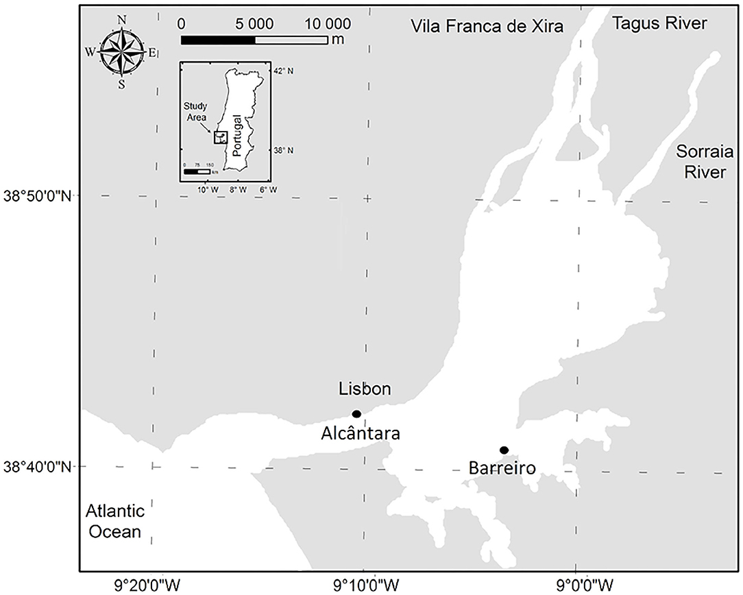
Figure 1. Geographic setting of the Tagus Estuary and the location of the sampling stations. Figure adapted from Brito et al. (2015).

A multiparameter probe (YSI EXO 2) was used to measure in situ temperature, salinity, pH, dissolved oxygen, and turbidity (in NTU) (Table 1). Vertical profiles were not performed as the Tagus Estuary is well mixed (Rodrigues and Fortunato, 2017), and these stations present low bottom depths (4–7 m). Secchi depth was assessed using a 50-cm white Secchi disk. Light extinction coefficient (Kd) was calculated by dividing 1.7 by the Secchi depth, as described in Tilzer (1988). A volume of 5 L of surface water was collected for analysis of (i) suspended particles, (ii) dissolved nutrients, and (iii) phytoplankton pigments. Water for nutrient analysis was filtered on-site with a hand filtration system using a precombusted (450°C for 4 h) 47-mm-diameter Whatman GF/C filter (Glass Fibber with 1.2 μm pore; Sigma Aldrich, St. Louis, MO, USA). These samples were then placed in a cooler, transported to the lab as soon as possible, and frozen at −20°C. Water for pigment analysis and suspended particulate matter (SPM) quantification were also placed in a cooler, protected from light and heat during transport to the lab, where they were processed.

TABLE 1

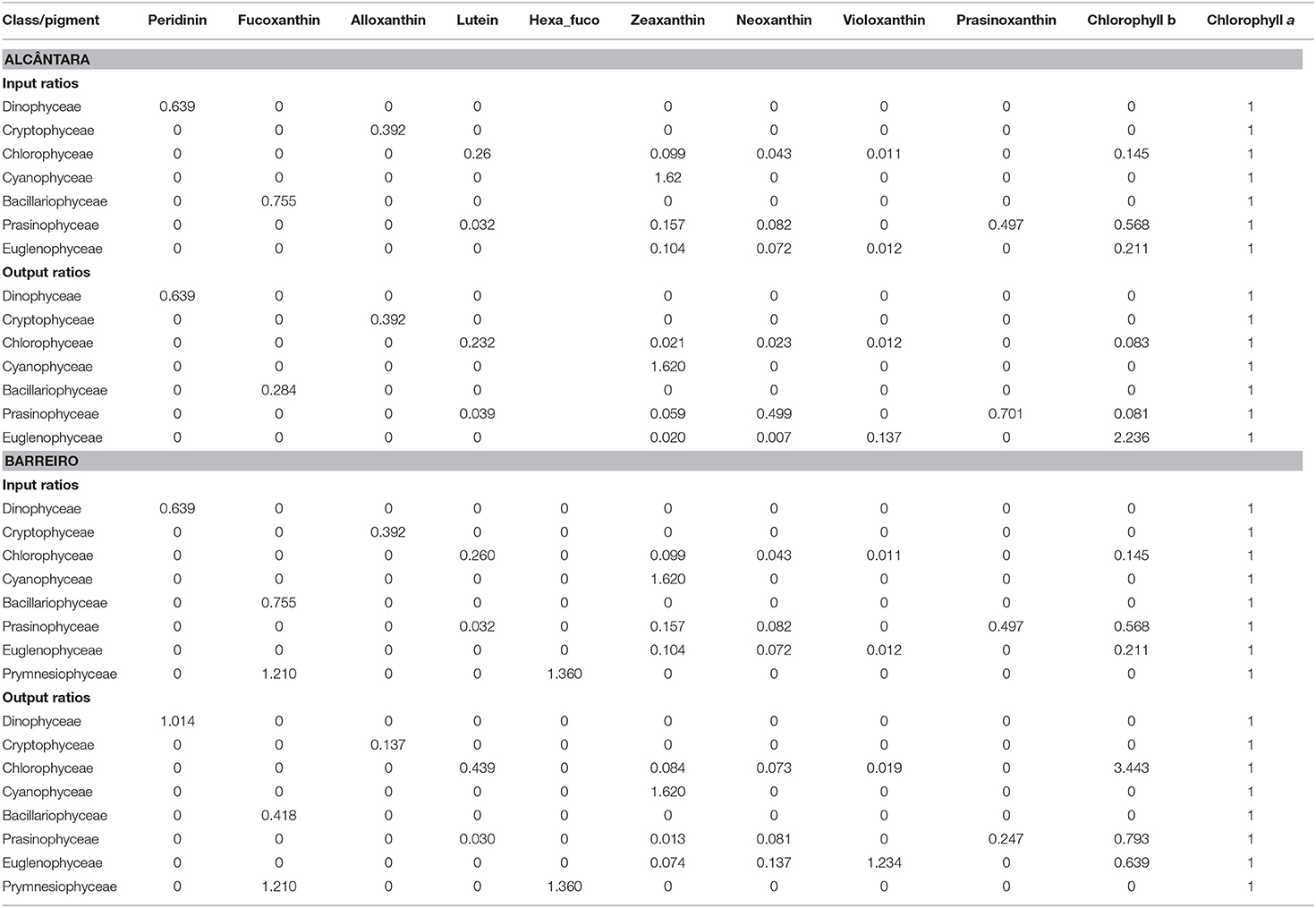
Table 1. Input and output ratios of marker pigments to chlorophyll a for Alcântara and Barreiro stations.

Weekly data on radiation (as weekly mean of total solar radiation per day), air temperature (both in Figure 2), and rainfall, as well as 5-day averages of river discharge (Figure 3) were gathered from Sistema Nacional de Informação de Recursos Hídricos [Sistema Nacional de Informação de Recursos Hídricos (SNIRH), 2019; www.snirh.pt].

FIGURE 2

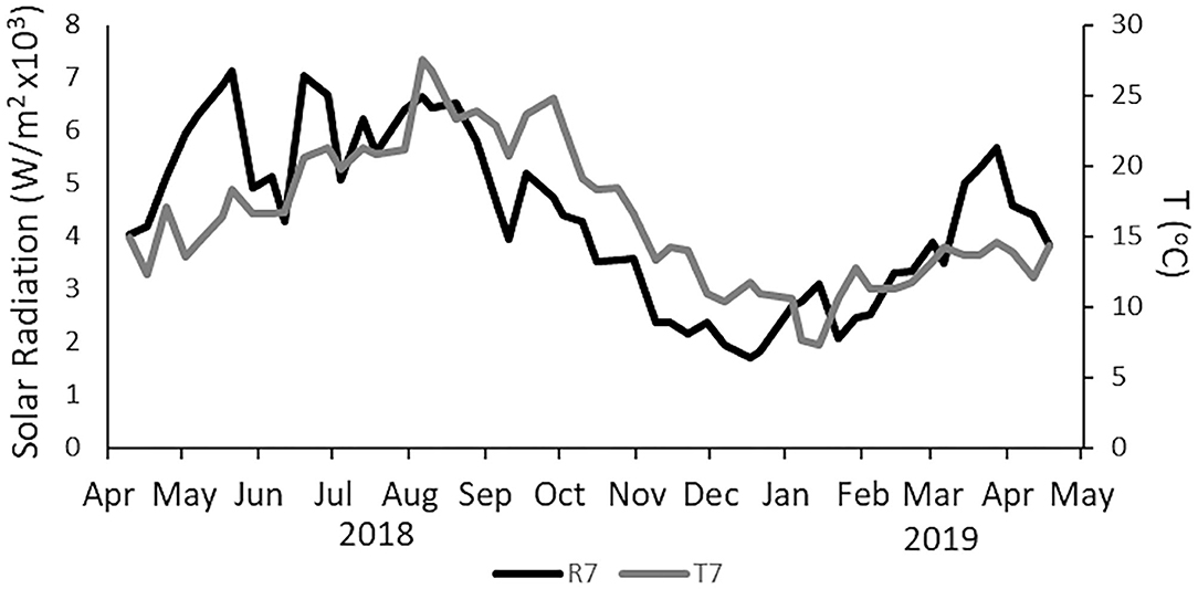
Figure 2. Weekly mean of total solar radiation per day (black line, responding to left side axis, on ×10³ W/m², radiation is expressed as the total radiation accumulated per day) and weekly mean temperature [light gray line, responding to right-side axis in degrees Celsius (°C)]. Data obtained from SNIRH (snirh.apambiente.pt) and measured at São João do Tojal meteorological station.

FIGURE 3

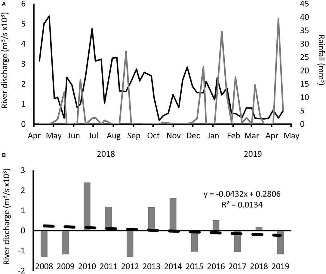
Figure 3. River discharge and rainfall in the Tagus Estuary. (A) Seven-day mean river discharge (black line) and 7-day total rainfall (gray line). (B) Yearly anomalies in relation to the global average using historical annual mean discharge from Almourol hydrometric station (data available since 1974) from SNIRH (snirh.apambiente.pt).

Analysis of Nutrient Concentrations

Triplicate samples for silicate, orthophosphate, nitrite, and nitrate concentrations were quantified through a TECATOR Flux Injection Analyzer FIA STAR 5000 (FOSS Tecator, Höganäs, Sweden) using the brand protocols. In the analyzer, nitrate was determined according to Grasshoff (1976), nitrite according to Bendschneider and Robinson (1952), and phosphates and silicates according to Murphy and Riley (1962) and Fanning and Pilson (1973), respectively. Ammonium concentrations were determined in triplicates, using manual colorimetric methods according to Koroleff (1969). DIN was computed as the sum of nitrite, nitrate, and ammonium concentrations.

Analysis of Suspended Particulate Matter and Organic Matter

For each sampling event, water for suspended particulate matter was filtered in triplicates using a precombusted (450°C for 4 h) 47-mm-diameter Whatman GF/C filter. After the sample filtration, 100 ml of ultra-pure water was passed through the filter to remove dissolved matter that would otherwise deposit in the filter, and the filter was stored in a drying oven at 60°C. Filters were allowed to dry for at least 24 h at 60°C and afterwards transferred to a desiccator to allow cooling. When resumed to room temperature, filters were weighted using a high precision scale. The weight of SPM (mg/L) is calculated by subtracting the weight of the filter before and after filtration. To quantify suspended organic (OM, mg/L) and inorganic matters (IM, mg/L), the filters were combusted at 450°C in order to extract the organic matter and weighed again. Organic matter is quantified by subtracting the weight of the filter after the last combustion to SPM. For inorganic matter, the weight of the combusted filter before filtration is subtracted to the weight of the filter after the last combustion.

Quantification of Phytoplankton Pigments

Phytoplankton pigments were quantified using two different methodologies: spectrophotometry and high-performance liquid chromatography (HPLC). HPLC analysis provided the full pigment signature of phytoplankton communities; however, only one sample was processed per station. For spectrophotometry, following the method proposed by Lorenzen (1967), to provide concentrations of chlorophyll a and phaeopigments, triplicate samples were used (for volumes, see Supplementary Table 1). Chlorophyll a data obtained from both methods presented the same temporal pattern and were almost identical (R² = 0.90, m = 1.06 and R² = 0.94, m = 1.03 for Alcântara and Barreiro, respectively). Given the different comparisons and statistical analyses conducted in this study, it was necessary to include both datasets. The spectrophotometric Chl a was used for the general phytoplankton biomass analysis while the HPLC chl a was only used for the community composition analysis. Water filtration was performed using 47 mm diameter (spectrophotometry) and 25 mm diameter (HPLC) GF/F Whatman filters (0.7 μm pore). Samples were stored at −80°C.

Quantification of Chlorophyll a and Phaeopigments by Spectrophotometry

Chlorophyll a and phaeopigment concentrations were estimated following the Lorenzen (1967) method. Extraction of pigments was performed by shredding the filters in 6 ml of acetone at 90% (v/v) dilution and left to rest at −20°C for 24 h. The samples were then centrifuged at 4,000 rpm for 15 min at 4°C. The supernatant was measured at 664 and 750 nm in a Shimadzu UV-260 UV-VIS spectrophotometer (Shimadzu, Kyoto, Japan). Measurements were taken before and after the addition of 12.5 μl of hydrochloric acid at 0.5 M to a 1-mL cuvette.

Quantification of Phytoplankton Pigments by HPLC and Chemotaxonomy

Pigment extraction and quantification was performed according to Gameiro et al. (2007) in a Shimadzu HPLC that is composed of a solvent delivery module (LC-10ADVP), a pump module (LC-10AD), a degasser module (DGU-14A), an oven module (CTO-10AS) and with system controller (SCL-10AVP), and a photodiode array (SPDM10AVP). Chromatography separation was performed using a C18 column for reversed-phase chromatography (Supelcosil, 0.46 25 cm, 5 mm particles; Sigma Aldrich, St. Louis, MO, USA). The solvent gradient followed Kraay et al. (1992) adapted by Brotas and Plante-Cuny (1996) with a flow rate of 0.6 m/min, an injection volume of 100 ml, and a duration of 35 min. Pigments were identified by comparing retention times and absorption spectra with pure crystalline standards from DHI. Pigment concentration was then calculated according to the following formula:

\begin{array}{l} P P (μg / L) = (\frac{S t}{S s}) \times (\frac{V m}{V f}) \times (A_{F P} \times m) \end{array}

In which PP is the concentration of a specific phytoplankton pigment (μg/L), St is the internal standard theoretical area, Ss is the internal standard sample area (both Ss and St are measured at the same wavelength of each pigment being quantified), Vm is the volume (ml) of extraction solution, Vf is the water volume filtered by the filter being analyzed, AFP is the absorbance for the desired pigment, and m is the slope of the calibration curve.

The relative composition of the phytoplankton groups was calculated using HPLC pigment concentration data and CHEMTAX chemical taxonomy software, version 1.95 (Mackey et al., 1996). CHEMTAX uses factor analysis and the steepest-descent algorithm to find the best fit of the data on an initial pigment ratio matrix. The method proposed by Latasa (2007) was then applied. This consists of performing subsequent CHEMTAX runs using the optimized pigment ratios resulting from the previous run. The main objective is to reduce the associated error to the minimum. Generally, the pigment ratios used were adapted from Gameiro et al. (2007). Moreover, for Barreiro samples, the ratios for Prymnesiophyceae presented by Mendes et al. (2011) were also added to respond to the presence of 19′-hexanoyloxyfucoxanthin. This pigment was not identified in Alcântara. Groups were defined using the taxonomic level “Class” and following the World Register of Marine Species (worms, at marinespecies.org, accessed on April 21, 2021). Input and output ratios are presented in Table 1.

Statistical Analysis

General Additive Models

The effect of physicochemical parameters on chlorophyll a concentrations were assessed using a generalized additive model with a cubic regression spline with K = 3. Due to the traditional F-like distribution of chlorophyll a concentrations, a Gamma distribution with a “log” link function was used in these models. Also, to assess how relative community composition changes due to environmental forcing, generalized additive models were performed, for the dominant or most relevant groups (Bacillariophyceae, Cryptophyceae, and Dinophyceae in both sampling sites and also for Prasinophyceae in Barreiro), with cubic regression splines with K = 3 and beta regression family with “identity” link function. In both general additive model (GAM) analyses, variables that present a sparse distribution on higher values were logarithmized to avoid problems in the model fit due to the higher importance attributed to single values on the extreme of the distribution. To assess the presence of multicollinearity between predictor variables, Spearman correlations were performed. Variables were excluded from the analysis when correlation was higher than 0.7 or worst concurvity was higher than 0.8. Correlations and concurvity values are presented in Supplementary Table 2. When a variable had to be removed, variables that have proved, in previous works, to be important in explaining chlorophyll a variations were maintained. Tidal height (for which sampling campaigns were also set) was not included as it was highly concurve with tidal range and, in Alcântara, also with nutrients. DIN and DSi presented high concurvity in Barreiro but were both kept since both are important to explain either chlorophyll concentration or group relative abundance. R software (R Core Team, 2019) was used to compute the models.

Truncated Fourier Series

To investigate the temporal variation of chlorophyll a concentrations, and due to the existence of missing values and irregular sampling intervals, a truncated Fourier series with M sets of sine–cosine waves have been fitted to the chlorophyll a data in function with time as described in Brito et al. (2012b). In this model, the lowest frequency (n = 1) represents the annual wave while the highest frequency (n = M) was set as 26, which comply with the Nyquist frequency limit (see Brito et al., 2012b for more information) and represents a periodicity of 15 days, which correspond to the tidal neap spring cycle. Afterwards, an analysis of variance was carried out to assess the relative importance of the seasonal cycle (represented by the wave-pairs 1–3), the higher-frequency temporal variation (wave-pairs 4 through 26) and the within-day variability in each component.

This model has the advantage of dealing with irregular sampling, by not employing the usual, but older methods (Chatfield, 2003) involving the successive fitting of sine–cosine pairs of increasing frequency (Brito et al., 2009). The Fourier analysis was performed using Matlab 2019A.

Results

Physicochemical Parameters

Temperature and radiation presented the typical seasonal pattern for temperate latitudes. The temperature increased from April to August, with the maximum weekly mean temperature (27.5°C) registered on August 6, 2018, decreasing from this point until January 14, when the minimum temperature was registered (Figure 2). Table 2 presents a summary of the physicochemical parameters, and the raw data is presented in Supplementary Table 3. Radiation increased from April to June when its maximum was registered (mean daily radiation of 7,111 W/m² on the week of May 21), and then decreased back until the minimum value registered on 21 of December (Figure 2). Alcântara presented the highest values for DIN, DIP, and suspended matter. Peaks in DIN concentrations, up to 200–500 μM, were frequently observed at Alcântara and were always related to peaks in DIP concentrations. At Barreiro, DIN concentrations varied between 15 and 35 μM, with two clear occasions, in May and August, where DIN concentrations decreased until almost 0 μM (Figures 4A,B). DIP concentrations in Alcântara were highly correlated with DIN (0.91, Supplementary Table 3; Figure 4C). At Barreiro, no correlation was found (0.39, Supplementary Table 3), although DIN reduction in August occurred simultaneously with a decrease of DIP and DSi concentrations to almost 0 μM (Figure 4D). Although the average concentrations of silicates were higher at Alcântara, observed values are relatively similar to the ones measured at Barreiro (Figures 4E,F, respectively). SPM was higher in Alcântara, and the concentration peaked during winter, from January to March. Regarding the Redfield ratios (Redfield, 1958; Brzezinski, 1985), Alcântara had most of the data points (73.8%) above the 16:1 DIN:DIP ratio, but only 7% over the 16:1 DSi:DIP ratio. Barreiro had 34% above the 16:1 DIN:DIP ratio, 9% over the 16:1 DSi:DIP ratio, and 4% above the 16:16:1 DSi:DIN:DIP (Supplementary Table 4; Figures 4I,J).

TABLE 2

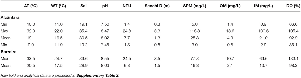
Table 2. Maximum, minimum, and mean for air temperature (AT), the water temperature at sampling (WT), salinity, pH, turbidity (NTU), Secchi depth (Secchi D), suspended particulate matter (SPM), suspended organic matter (OM), suspended inorganic matter (IM), dissolved oxygen saturation DO (%), and concentration of dissolved oxygen.

FIGURE 4

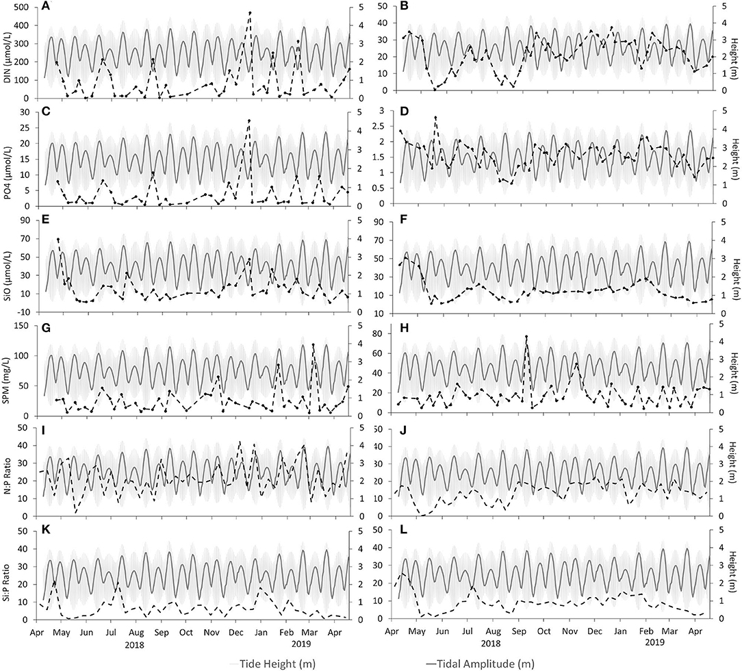
Figure 4. Nutrients and suspended particulate matter for the sampling period, plotted against tidal cycle (light gray shade on the back) and tidal range (gray line). The dotted lines represent, for Alcântara (left) and Barreiro (right), of which graphs (A,B) present dissolved inorganic nitrogen in micromoles per liter, (C,D) present the concentrations of orthophosphate (DIP) in micromoles per liter, (E,F) present the concentration of silicates (SiO) in micromoles per liter, (G,H) present the concentrations of suspended particulate matter (SPM) in milligrams per liter, and (I–L) present the nutrient ratio DIN:DIP and DSi:DIP.

Phytoplankton Biomass (Chlorophyll a)

Chlorophyll a concentrations varied between 0.5 and 6.2 μg/L in Alcântara and 0.6 and 11.3 μg/L in Barreiro (Figures 5A,B). The seasonal pattern observed at both stations has common features, namely two peaks of chlorophyll a: (i) the first observed in spring, starting in mid-May 2018 and lasting until mid-June 2018 at Barreiro and end of June at Alcântara and (ii) the second in summer, in early August. However, distinct features were registered between the two sites; in particular, there were two other peaks in Alcântara, not observed in Barreiro, in October 2018 and March 2019.

FIGURE 5

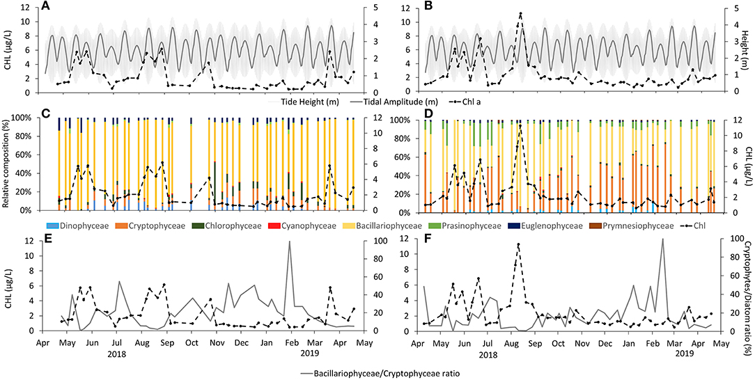
Figure 5. Chlorophyll a (quantified by spectrophotometer) distribution at (A) Alcântara (left side) and (B) Barreiro (right side) compared with tidal height (gray shade) and tidal range (gray line); in (C,D) with relative community composition quantified by HPLC and CHEMTAX and in (E,F) with Bacillariophyceae/Cryptophyceae ratio.

Phytoplankton Community Composition

In terms of phytoplankton community composition, it was possible to observe that Bacillariophyceae dominated the phytoplankton community in Alcântara throughout the year (up to 100% and a mean of 76% of the community, Figure 5). Other important groups in Alcântara were Chlorophyceae (up to 45% and mean of 5% of the community in October 2018), Cryptophyceae (up to 24% and mean of 8% of the community), and Dinophyceae with a maximum of 15% and mean of 4% of the community registered in September. In general, at Barreiro, Bacillariophyceae were also dominant (up to 97% and mean of 52% of the community, Figure 4), followed by Cryptophyceae (up to 74% and mean of 35% of the community) and Prasinophyceae (that represented up to 31% and a mean of 8% of the community). At both sampling sites, Bacillariophyceae clearly dominated the phytoplankton community when a chlorophyll a peak was observed (Figure 5).

In terms of tidal conditions, Bacillariophyceae presented stronger dominance during spring tides with up to 99 and 96% and a mean of 82 and 58% of the community at spring tides, in Alcântara and Barreiro, respectively. During neap tides, Bacillariophyceae represented up to 96% of the community in Alcântara and 91% at Barreiro, with associated means of 71 and 45% at Alcântara and Barreiro, respectively. Cryptophyceae presented the opposite trend with higher values during spring tides, representing up to 14 and 61% and means of 7 and 31% of the community for Alcântara and Barreiro. At neap tides, Cryptophyceae composed up to 24 and 74% and a mean of 9 and 40% of the community for Alcântara and Barreiro, respectively (Figure 6).

FIGURE 6

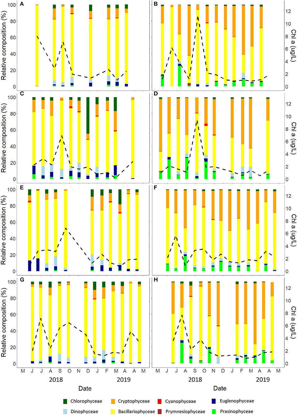
Figure 6. Community composition determined by CHEMTAX and expressed on micrograms per liter of chlorophyll a for Alcântara (left side) and Barreiro (right side) for spring high tide (A,B), neap high tide (C,D), neap low tide (E,F), and spring low tide (G,H).

Effect of the Spring-Neap Tidal Cycle on Phytoplankton Biomass

A Fourier analysis considering a maximum of 26 wave-pairs were found to be highly explicative for both Alcântara and Barreiro (92 and 90% of variance explained, respectively; Table 3; Figure 7). A good temporal agreement between model output, considering 26 wave-pairs, and data points were observed (Figure 7) for both sites. The seasonal cycle (1–3 waves) explained 37% of the variance at Alcântara. The higher-frequency temporal variation corresponding to a period down to 14 days, representing the spring vs. neap variation (4–26 waves) explained an additional 55% of the variance. At Barreiro, the results are very similar. The seasonal component explained 36% of the variance and an additional 54% were explained by fitting 4 to 26 waves (n). Fits were significant at a significance level of 0.05 (p < 0.001 for both Alcântara and Barreiro fits), which was used for all analyses.

TABLE 3

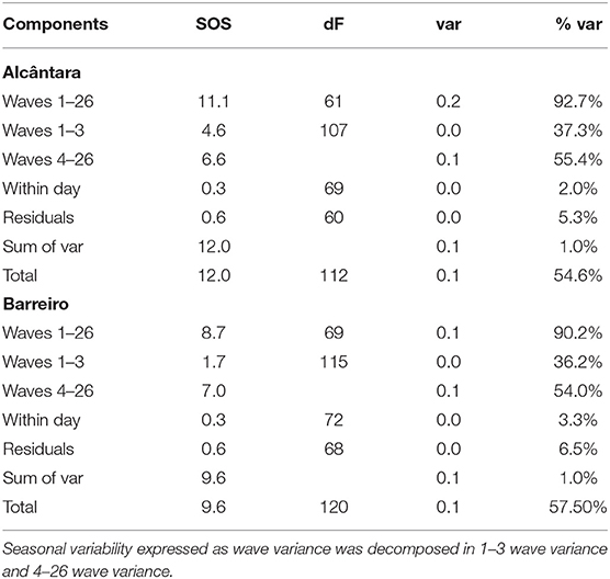
Table 3. Sum of squares (SOS), degrees of freedom (dF), variance (var), and percentage of explained variance (% var) of the three main components (waves, within day, and residuals) and totals.

FIGURE 7

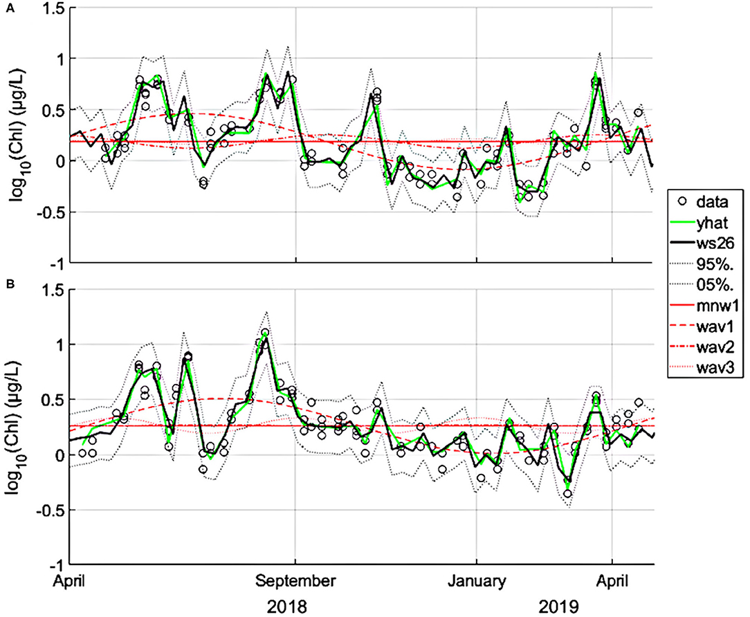
Figure 7. Seasonal pattern of chlorophyll a for Alcântara (A) and Barreiro (B), obtained by fitting 26 wave-pairs (sine–cosine) according to the truncated Fourier series approach. Log-transformed data are presented as dots. The 5 and 95% confidence intervals are represented as dotted black lines. The green line (yhat) is the equivalent to the sum of waves (ws) but adjusted for a time step that is coincident with the sampling date. Waves 1–3 (annual and seasonal variations) are presented as dashed and dotted red lines.

Assessment of Main Drivers of Phytoplankton Variability

The application of the GAM model to the chlorophyll a data, as a proxy of phytoplankton biomass, revealed a significant influence of several variables, such as the following: tidal range, water temperature, salinity, silicate concentration, DIN concentration, and river discharge. Salinity and river discharge values were higher during spring (Figure 3; Table 4). In Alcântara, chlorophyll a concentrations increased with tidal range and water temperature. Higher chlorophyll a concentrations were found to be associated with lower salinity (which was observed during spring), low silicate concentrations, low river discharges, and extreme values (both high and low) of DIN (Table 5; Supplementary Figure 1). For Barreiro, the main drivers of chlorophyll a concentrations were water temperature, pH, tidal range, silicate concentration, and solar radiation (Table 4). Of these, tidal range, water temperature, and salinity influenced the chlorophyll a concentrations with the same patterns observed in Alcântara (Table 5).

TABLE 4

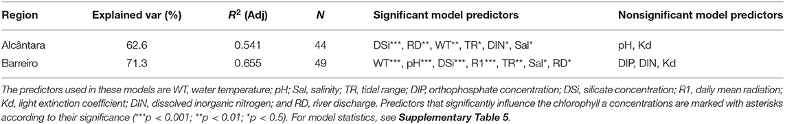
Table 4. Predictors and p-value for generalized additive models for Alcântara and Barreiro.

TABLE 5

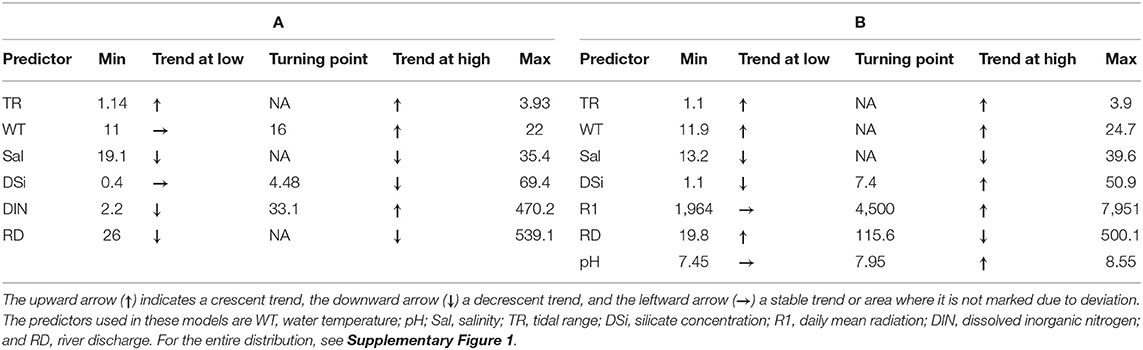
Table 5. Summary of the relationship between the predictor variables and chlorophyll a from minimum to a turning point in the trend (if any) and from there to maximum values of the predictor variable.

Additionally, high chlorophyll a concentrations were observed in association with high values of pH and solar radiation, particularly during late spring and summer (Table 5; Supplementary Figure 1).

Results from GAMs applied to groups are presented in Tables 6, 7, as well as in Supplementary Figure 2. General additive models show that, in Alcântara, Bacillariophyceae composition was positively related with tidal range and water temperature, while being negatively influenced by silicate concentration and river discharge. Cryptophyceae were significantly influenced by tidal range, water temperature, DIN, and silicate concentration and river discharge with all the variables presenting an inverse pattern to that found for the Bacillariophyceae. Dinophyceae presented significant differences only with river discharge, which increased their representativity from lower to medium values of river discharge but had no effect in higher values.

TABLE 6

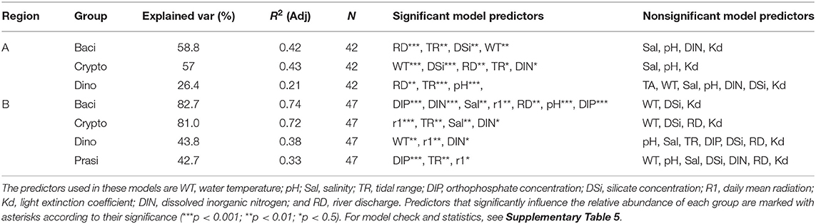
Table 6. Beta regression generalized additive model fit to each of the dominant groups (Bacillariophyceae, Cryptophyceae, and Prasinophyceae as Diato, Crypto, and Prasino, respectively) and Dinophyceae (as Dino) using cubic regression splines and K = 3.

TABLE 7

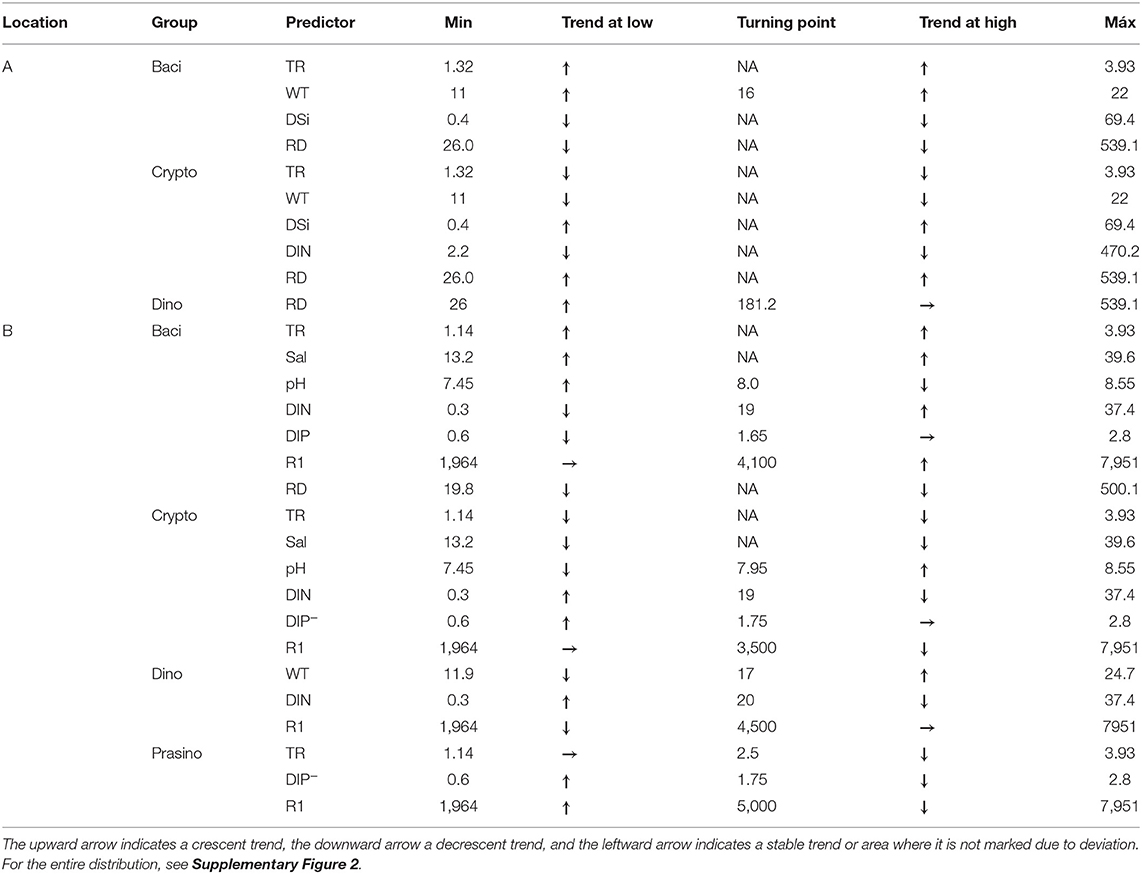
Table 7. Summary of the relation between the predictor variables and the phytoplankton groups from its minimum to a turning point in the trend (if any) and from there to the maximum of the predictor variable.

At Barreiro, the tidal range was the only variable that presented the same pattern of Alcântara for the different taxonomic groups. At Barreiro, Bacillariophyceae had a positive relationship with salinity, tidal range, and high values of solar radiation. Also, Bacillariophyceae were higher for median values of pH (maximum at around 8 of pH) and at extreme values of DIN (minimum at 20 μmol/L). In relation to DIP, Bacillariophyceae were higher when low concentrations of this nutrient were detected, presenting also a slight increase at high values (minimum at 1.7 μmol/L). Cryptophyceae were significantly influenced by water temperature, pH, salinity, tidal range, DIP, DIN, and solar radiation, from which all except water temperature (not significant for Bacillariophyceae) followed the opposite trend of that registered for Bacillariophyceae. In relation to water temperature, Cryptophyceae were negatively influenced by this variable, decreasing with warmer waters. Dinophyceae were significantly influenced by water temperature, tidal range, solar radiation, DIN, and SPM. From these, tidal range, solar radiation, and DIN presented an inverse pattern when compared with Bacillariophyceae. The importance of this phytoplankton class increased when the water temperature was higher than 17°C and lower than 16°C. Prasinophyceae representativity in the community was significantly influenced by tidal range, DIP, and solar radiation. Their importance decreased at high values of the tidal range being stable at ranges under 2.5 m. Also, higher percentages of Prasinophyceae were associated with medium values of both DIP and radiation (maxima at around 1.75 μmol/L of DIP and 5,000 W/m² of radiation).

Discussion

Environmental Patterns in the Tagus Estuary

In previous studies, nutrient variability in the Tagus Estuary presented a seasonal trend, with maximal concentrations of dissolved inorganic nitrogen (DIN) and silicates during the winter–spring period. This is likely a consequence of their freshwater origin together with the decreased biomass of phytoplankton that is registered during winter, increasing again in the spring (Gameiro et al., 2007; Borges et al., 2020). Phosphates have also presented maximum values in summer, potentially due to the increase in water temperature during the summer that promotes the release of phosphate from the sediment (Gameiro et al., 2011; Borges et al., 2020). In estuaries, a decrease in turbidity, suspended matter, nutrients, and chlorophyll a from the turbidity maximum toward the estuary mouth is generally observed (conservative mixing) (Vale and Sundby, 1987; Cabeçadas et al., 1999; Garnier et al., 2010; Liang et al., 2013). Conservative mixing has been verified in several systems, such as the Scheldt (Soetaert et al., 2006), Lojn, Ems, and Douro estuaries, and occasionally also in the Girone Estuary (Lemaire et al., 2002; Azevedo et al., 2008). The Tagus Estuary presents its turbidity maximum around 30 to 50 km upstream of the estuary mouth, thus located upstream of the sampling stations of the present study (Vale and Sundby, 1987; Vale, 1990). In this work, the concentrations of nutrients, SPM and chlorophyll a observed at Barreiro were within the expected range for this location (SNIRH.pt accessed on February 18, 2021), being lower than the ones found in upstream areas (Gameiro et al., 2007; Gameiro and Brotas, 2010; Brito et al., 2012a). However, at Alcântara, a different situation was observed. The lowest values of chlorophyll a and DIP, as well as the maximum value for Secchi Depth, were observed at Alcântara. On the other hand, Alcântara also presented higher mean and maximum values of DIP, DIN, and suspended matter concentrations than those observed at the Barreiro sampling station. These values were also higher than the ones recorded in previous studies upstream in the estuary (Gameiro et al., 2007; Gameiro and Brotas, 2010; Brito et al., 2012a), which did not comply with the conservative mixing. Such higher concentrations were mainly detected during low tides while the lower nutrient concentrations were found during high tides. This divergence of the conservative mixing is probably a consequence of the proximity to a sewage treatment station outfall. Sewage discharges enhance both DIN and DIP while having a reduced effect on Si (Struyf et al., 2004; Caetano et al., 2016; Maguire and Fulweiler, 2016). Such associations between outfalls and the increase in inorganic forms of N and P have been verified in many European estuaries, such as the Ria de Aveiro (Lopes et al., 2007) and Forth estuary (Balls, 1990). In Alcântara, ammonium, nitrite, nitrate, and orthophosphate concentrations were highly correlated and presented high concentrations. Si, which is mainly originated by rock weathering (Treguer et al., 1995; Garnier et al., 2002), had concentrations that were within the range of values previously reported for the estuary (SNIRH.pt, accessed on February 1, 2020). In this case, during low tides, the water body is influenced by the water coming from the outfall. However, at high tide, the large volume of coastal water (poor in nutrients and turbidity) entering the estuary is bound to dissipate the outfall influence over this sampling location. Such effect may also have been magnified by the fact that the sampling was performed from land, and particularly, near the outfall. These stations had only 5–10 m depth in the low tide. Previous studies have verified that the sewage plume tends to be more noticeable closer to the margin (Costa et al., 2012). Therefore, if sampling is performed further away from the shoreline, where the bottom depth is higher, these differences are expected to be much smaller.

Temporal Variation of Phytoplankton Biomass as a Function of Its Drivers

Regarding annual variability, chlorophyll a presented a similar pattern in both sampling stations, yielding peaks in phytoplankton biomass from May to the end of June and in August. Afterwards, from October to March, chlorophyll a concentrations remained below 2 μg/L. Such temporal variability was identified by the first three waves of the Fourier analysis, explaining 37.2 and 36.2% of the data variability for Alcântara and Barreiro, respectively. The importance of seasonal effects on chlorophyll a is well-described in the literature as a common feature in estuarine and coastal waters (Iriarte and Purdie, 2004; Shen et al., 2011; Carstensen et al., 2015), as well as for the Tagus (Gameiro et al., 2007). In the Tagus Estuary, an increase in chlorophyll a is reported in spring and summer by several authors (Mateus and Neves, 2008; Gameiro and Brotas, 2010; Gameiro et al., 2011; Brito et al., 2012a). Still, as verified in the results presented herein, seasonal variations only accounted for a small part of the chlorophyll a variability, meaning that other periodic drivers were more relevant to chlorophyll a.

GAM analysis computed the relationship between chlorophyll a concentration and the variables that represented the seasonal variability: temperature and solar radiation (in Alcântara these parameters were highly correlated). Besides seasonal variables, also nutrients, salinity, and turbidity have been considered as important drivers of variation on phytoplankton biomass in the Tagus Estuary (Brogueira et al., 2007; Gameiro et al., 2007; Saraiva et al., 2007). In the present work, both salinity and nutrients were found to have a significant influence on chlorophyll a concentration at both sampling stations. Due to the location of these sampling stations in the lower estuary, silicate is probably being consumed upwards of these stations. Still, and although the correlation between discharges and silicate concentration was low, it is possible to observe that low silicate concentrations are coincident with low river discharge situations. In fact, although 2018 was not an extremely dry year for the area of the Tagus Estuary, 2019 was a dry year (Pordata.pt, accessed on February 2, 2020) (Base de dados de Portugal Contemporânio, 2020). As a consequence, a reduction in the river discharge in the final sampling months is clearly seen. The Tagus river discharges are greatly influenced by several dams along the river course. López-Moreno et al. (2009) noticed that dams reduce the seasonal effect of rain by decreasing the water flow in the winter and increasing it in the summer. In the same study, it is noticed that dams have the effect of increasing drought in areas downstream of their walls. Also, during the sampling period (spring 2018 to spring 2019), parts of the Iberian Peninsula were under drought, hence it is likely that large amounts of water could have been transferred from the Tagus to smaller rivers, a common procedure in dry years (Morote et al., 2019). Such reduction in freshwater discharges leads to a reduction in the entrance of silicates to the estuary (Rodrigues et al., 2019). As the Estuarine Turbidity Maximum is dependent on salinity, it may be forced upstream, which can promote phytoplankton growth in the lower areas of the estuary, leading to an increase in nutrient assimilation. The reduction in the freshwater input, and consequently in the DSi concentrations, can also lead to changes in the phytoplankton community (Rocha et al., 2002; Domingues et al., 2008, 2015). Effects of silicate reduction on the phytoplankton biomass and community succession has also been registered in several systems such as the Curonian Lagoon, in the Baltic Sea (Pilkaityte and Razinkovas, 2006), Moreton Bay (Glibert et al., 2006), and Pearl River Estuary (Yin et al., 2000).

The Fourier series analysis also indicated that high-frequency processes, up to 26 waves (i.e., 15-day variation) explained up to 55 and 58% of phytoplankton variability in Alcântara and Barreiro, respectively. The influence of the tidal range, which presents a periodicity of 15 days, on the phytoplankton dynamics has been well described in other estuaries and enclosed waters (Cloern, 1991; Gianesella et al., 2000; Azhikodan and Yokoyama, 2016). Generally, this relationship is driven by changes in the residence time and in the dilution effect due to the entrance of coastal waters, with higher chlorophyll a concentrations usually associated with neap tides. Monbet (1992) analyzed the influence of the neap-spring tidal cycle, conducting a metaanalysis with several estuaries around the world (including the Tagus Estuary) and suggested that the lower chlorophyll a concentrations should be observed during spring tides, as a consequence of the higher mixing during such tidal conditions that can drag the phytoplankton cells under the photic layer. In fact, the tidal range effect over chlorophyll was significant at both stations, presenting an increase in chlorophyll a at higher tidal range (spring tides). Given that higher tidal ranges are likely to be associated with lower residence times and higher turbidity, this seems to be in disagreement with what was previously described in the literature, i.e., an association between higher chlorophyll a concentration with higher residence times caused by neap tides (Cloern, 1991; Lucas et al., 1999; Trigueros and Orive, 2000). This is probably a combination of the well-flushed nature of the low and mid-Tagus Estuary, with the large extent of highly productive mudflats present in the mid-estuary (Brotas and Catarino, 1995; Rodrigues and Fortunato, 2017). Nevertheless, it is important to note that the residence time in the Tagus results from the joint action of several factors, such as tide, river flow and wind (Oliveira and Baptista, 1998; Braunschweig et al., 2003; Vaz and Dias, 2014) that adds complexity to the analysis. In addition, such an increase in chlorophyll a concentrations does not seem to result from changes in light availability during spring tides since turbidity increases during such tidal conditions due to the resuspension of sediments (Vale and Sundby, 1987). This resuspension is a common feature of highly turbid estuaries (De Jorge and Van Beusekom, 1995; Gianesella et al., 2000; Ubertini et al., 2012) and contributes to the increase in photosynthetic biomass by the resuspension of microphytobenthos (Brotas et al., 1995; Cabrita and Brotas, 2000; Jesus et al., 2009). The importance of tide in resuspending microphytobenthos and its association with SPM have been observed in other systems (Brito et al., 2012b, Redzuan and Underwood, 2021). In this case, the resuspension of sediments by the stronger currents of the spring tides could be the cause for the increase in the chlorophyll a in the water column. In the mid part of the Tagus Estuary, Brito et al. (2015) reported high numbers of several diatom species usually associated with microphytobenthos, such as Navicula sp. and Diploneis sp. In the future, additional microscopy analysis could provide valuable information to confirm such hypotheses for these locations.

Community Composition

General Patterns of Community Composition

In estuaries, the dominance of Bacillariophyceae over small flagellates is considered an indicator of a good environmental state (Devlin et al., 2012; Ferreira et al., 2017) and is found in many of the European estuaries as, the Krka Estuary (Cetinić et al., 2006), Schelde Estuary, Elbe Estuary (Muylaert and Sabbe, 1996), Ria de Aveiro (Lopes et al., 2007), and Guadiana Estuary (Rocha et al., 2002; Domingues et al., 2005). Bacillariophyceae has been recorded as the main bloomers in the mid-Tagus Estuary (Gameiro and Brotas, 2010). In a recent period (2006–2007), Brito et al. (2015) reported a reduction in Bacillariophyceae dominance in favor of Cryptophyceae. The authors suggested that this shift could be caused by a top–down effect due to the increase of the invasive clam Ruditapes philippinarum. Grazing is known for being able to shape the estuarine phytoplankton community (Lonsdale et al., 1996; Cloern, 2018). Bacillariophyceae are more edible for organisms at higher trophic levels, such as large fish and shellfish (Officer and Ryther, 1980; National Research Council, 1993). The influence of bivalve grazing over the community greatly varies with the system in analysis. Jones et al. (2017), analyzing the bivalve grazing effect on the food web in Whangateau Harbor, verified that its effect was higher over microphytobenthos than over pelagic species. On the other hand, Jiang et al. (2020) verified that grazing was one of the dominant drivers of phytoplankton spatial variability at Eastern Scheldt. Such relationships still need to be shown for the Tagus Estuary, but the continuous monitoring program that has been performed for 20 years in the mid-Tagus Estruary does not show a clear shift from Bacillariophyceae to Cryptophyceae in the latest years (Tracana and Brotas, 2019). In the present work, Bacillariophyceae were the dominant group in both sampling sites with Cryptophyceae being the second most important group, presenting small importance in Alcântara. Gameiro et al. (2007), which also used CHEMTAX to evaluate the community composition, observed a decrease in Bacillariophyceae and Chlorophyceae importance in the community from upstream to downstream with Cryptophyceae, Prasinophyceae, and Dinophyceae gaining importance toward downstream areas. Barreiro sampling station presented a similar trend with higher importance of Cryptophyceae and Prasinophyceae than that found in the central zone of the estuary by Gameiro et al. (2007). In contrast, the Alcântara community was almost entirely composed of Bacillariophyceae in most of the sampling occasions. Such high Bacillariophyceae dominance in comparison with the mid-estuary (Gameiro et al., 2007) is probably due to the higher influence of coastal waters dominated by Bacillariophyceae species, such as Detonula pumila and Thalassiosira sp. These taxa are dominant in the nearby Cascais Bay (Silva et al., 2009) and are carried to the estuary due to the strong currents observed in this area (Fortunato et al., 1997; Guerreiro et al., 2015). Chlorophyceae presented small importance in both Alcântara and Barreiro probably due to its freshwater origin (Cetinić et al., 2006; Gameiro et al., 2007).

Main Drivers of Variability in Community Composition

Seasonal drivers (i.e., radiation and water temperature), nutrients availability (Si and DIN in Alcântara and DIN and PO4 in Barreiro), tidal range, and river discharges explained variations in the phytoplankton community at both sampling stations. The Bacillariophyceae yielded a variation pattern that was similar to that described for chlorophyll a, indicating that Bacillariophyceae were the main group contributing to its variations. In many estuaries, phytoplankton seasonality is characterized as having a higher percentage of Bacillariophyceae from autumn to early spring with an increase in the flagellate fraction during summer, as seen in Ria de Aveiro (Lopes et al., 2007) and Guadiana Estuary (Rocha et al., 2002; Domingues et al., 2005). In this study, such a pattern was not observed as diatoms presented higher percentages during summer. In fact, Gameiro et al. (2007) has reported high flagellate contributions to the community at some stations during winter and autumn, presenting great annual variability. The Cryptophyceae presented a significant variation with almost all the same variables as Bacillariophyceae, but with opposite trends, meaning that they can benefit from conditions that are not the most adequate for Bacillariophyceae. Dinophyceae and Prasinophyceae were less represented, but, in general, also followed the opposite trend when compared with Bacillariophyceae.

The negative relationship between Bacillariophyceae and river discharge is a consequence of seasonality, due to higher river discharges in early spring. Nutrients were also important in explaining the changes in groups, with DSi concentrations presenting an inverse relationship with Bacillariophyceae in Alcântara while in Barreiro an inverse association with nutrients was detected with both DIN and DIP (MATLAB, 2019). Such trends may also be a consequence of seasonality due to lower nutrient concentrations during summer when nutrients are low due to high consumption and low riverine nutrient input. In Alcântara, the pattern is mostly influenced by the outfall introducing high concentrations of DIN and DIP with Bacillariophyceae responding only to DSi. Due to the association of nutrients with the river discharges, it is important to assess in future works what changes in the hydrologic regime can influence the community composition of the Tagus Estuary, as well as maintaining a concise monitoring of the phytoplankton community composition. Shifts in the phytoplankton community can facilitate the blooming of harmful algae bloom and influence phytoplankton biomass. Also, the change in the dominance from Bacillariophyceae to flagellate taxa can affect the estuarine food-web as diatoms are more easily digested by large filter feeders that usually are the link to higher trophic levels (Officer and Ryther, 1980; Managing Wastewater in Coastal Urban Areas, 1993).

The positive relation between Bacillariophyceae and tidal range follows the variations observed for chlorophyll and is likely to result from a combination of factors, in which microphytobenthos resuspension and the higher penetration of coastal water rich in Bacillariophyceae, should play a crucial role. In Barreiro, due to the extension of the mudflat areas in mid-estuary, microphytobenthos should make a relevant contribution to overall chlorophyll a during spring tides. The coupling between microphytobenthos and pelagic microalgae can be an important characteristic of the estuary, as indicated by the presence of microphytobenthos species in phytoplankton (Brotas and Catarino, 1995; Gameiro et al., 2011; Brito et al., 2012b). During spring tides, the strong currents registered in the estuary would not only resuspend microphytobenthos but also reduce the sinking rate, allowing heavier cells, such as Bacillariophyceae, to easily avoid sedimentation. In Alcântara the main factor contributing to the Bacillariophyceae dominance was probably the proximity to coastal waters and the higher water mixing during spring tides. Additionally, this is in accordance with the study of Margalef (1978) that indicated that Bacillariophyceae are positively influenced by high values of nutrients and mixing, while Cryptophyceae prefer more stratified low-nutrient waters.

Conclusions

In summary, the phytoplankton community in the Tagus Estuary was greatly influenced by two main factors: seasonality and tidal range. The fortnight tidal cycle explained most of the variability. This is a key finding for this study, indicating the relevance of taking into spring-neap tidal cycles in estuarine assessments of water quality. In addition, higher phytoplankton biomass, associated with higher dominance of Bacillariophyceae in the community, was mainly observed during spring tides. Bacillariophyceae seems to be the group that contributes the most to the overall phytoplankton biomass in the Tagus Estuary. In Alcântara, the physicochemical parameters (i.e., nutrients and SPM) presented strong variations in the spring-neap tidal cycle, probably due to the presence of an outfall. The results presented in this work reinforce the need to assess the influence of the tidal cycle to fully understand ecosystem functioning in estuaries. This is also key to evaluate how the tidal effect influences water quality classifications, as well as investigate how climate change will affect estuarine systems in the near future.

Data Availability Statement

The original contributions presented in the study are included in the article/Supplementary Materials, further inquiries can be directed to the corresponding author.

Author Contributions

RC performed the sampling campaigns and laboratory analysis, performed the statistical analysis and image formatting, and is the main writer of the document. VB contributed with the idea and together with AB and MR planed the sampling campaigns, acquired the necessary resources, and reviewed the document and statistics. JC helped on the sampling campaigns, performed laboratory analysis, and reviewed the CHEMTAX procedure and the document. All authors contributed to manuscript revision, read, and approved the submitted version.

Funding

The authors acknowledge Andreia Tracana, Pedro Oliveira, and Joshua Heumüller for their support in field campaigns and data analysis. In addition, the authors are grateful to Administração do Porto de Lisboa (APL) and Serviço de Estrageiros e Fronteiras (SEF) for allowing access to Alcântara harbor. RC and AB received funding from Fundação para a Ciência (FCT) e a Tecnologia (PD/BD/135064/2017 and CEECIND/00095/2017, respectively). This work received further support from the following projects: UBEST (PTDC/AAGMAA/6899/2014) funded by FCT; Infrastructure CoastNet (http://geoportal.coastnet.pt) funded by FCT, and the European Regional Development Fund (FEDER) through LISBOA2020 and ALENTEJO2020 regional operational programs, in the framework of the National Roadmap of Research Infrastructures of strategic relevance (PINFRA/22128/2016); MARE Center strategic grant (UIDB/04292/2020); and IDL strategic grant (UIDB/50019/2020), also granted by FCT. This work was funded by the Copernicus Evolution: Research for Harmonized Transitional Water Observation (CERTO) under the European Union's Horizon 2020 Research and Innovation Programme, Grant No. 870349 and was also supported by funding from the European Union's Horizon 2020 Research and Innovation Programme under grant agreement N810139: Project Portugal Twinning for Innovation and Excellence in Marine Science and Earth Observation (PORTWIMS).

Conflict of Interest

The authors declare that the research was conducted in the absence of any commercial or financial relationships that could be construed as a potential conflict of interest.

Supplementary Material

The Supplementary Material for this article can be found online at: https://www.frontiersin.org/articles/10.3389/fmars.2021.675699/full#supplementary-material

References

Agência Portuguesa do Ambiente (2016). Plano de Gestão da Região Hidrográfica, RH5, Parte 2 – Caracterização e Diagnostico. Lisbon: Agência Portuguesa do Ambiente.

Azevedo, I. C., Duarte, P. M., and Bordalo, A. A. (2008). Understanding spatial and temporal dynamics of key environmental characteristics in a mesotidal Atlantic estuary (Douro, NW Portugal). Estuar. Coast. Shelf Sci. 76, 620–633. doi: 10.1016/j.ecss.2007.07.034