 Ibrahim M. Ghandour1
 Aaid G. Al-Zubieri1*
 Ali S. Basaham1Ammar A. Mannaa1Talha A. Al-Dubai2
 Brian G. Jones3
- 1Department of Marine Geology, Faculty of Marine Sciences, King Abdulaziz University, Jeddah, Saudi Arabia
- 2Department of Marine Geology, Faculty of Marine Sciences and Environments, Hodeidah University, Al Hudaydah, Yemen
- 3School of Earth, Atmospheric and Life Sciences, University of Wollongong, Wollongong, NSW, Australia
Late Quaternary paleoenvironments are of particular interest to understand how the Earth System’s climate will respond to the undramatic changes during this period, compared with the broader glacial-interglacial variations. In this study, a shallow sediment core (2.84 m long) retrieved from the Red Sea coastal zone in northern Ghubbat al Mahasin, south of Al-Lith, Saudi Arabia, is used to reconstruct the mid-Late Holocene paleoenvironments and sea level based on a multiproxy approach. Remote sensing data, sedimentary facies, benthic foraminiferal assemblages, δ18O and δ13C stable isotopes, elemental composition and 14C dating were utilized. The stratigraphy of the core shows three distinctive depositional units. The basal pre 6000 year BP unit consists of unfossiliferous fine to medium sand sharply overlain by black carbonaceous mud and peat, suggesting deposition in a coastal/flood plain under a warm and humid climate. The middle unit (6000-3700 year BP) records the start and end of the marine transgression in this area. It consists of gray argillaceous sand containing bivalve and gastropod shell fragments and a benthic foraminiferal assemblage attesting a lagoonal or quiet shallow marine environment. The upper unit (<3700 year BP) consists of unfossiliferous yellowish-brown argillaceous fine-grained sands deposited on an intertidal flat. Both middle-and upper-units stack in a regressive shallowing upward pattern although they may be separated by a hiatus. The overall regressive facies and the stable isotopic data are consistent with a late Holocene sea-level fall and a change to a more arid climate.
Introduction
Paleoenvironmental reconstruction of coastal deposits is a critical key for assessing climatic and sea level changes that occur as a response to allogenic processes operating at global to regional scales, and the action of autogenic processes at local scales (Hein et al., 2016). Coastal deposits are situated at the interface between terrestrial and marine environments and contain fingerprints of recent climate fluctuations and human civilization development, which are possibly useful for improving climate prediction models and enhancing sustainable development in coastal ecosystems (Padmalal et al., 2014a). Consequently, the Holocene sea-level and climate archives have gained considerable interest in several scientific studies (Lambeck, 1997; Hayward, 1999; Proust et al., 2010; Moreno et al., 2014; Durand et al., 2016; Bulian et al., 2019). According to several authors, the global climate during the Holocene is divided into three main stages: Early, mid and Late Holocene. The early period was characterized by frequent drought events and a more or less steady rise in sea-level following the Last Glacial Maximum (Bulian et al., 2019). For example, Siddall et al. (2003) stated that the rate of sea-level change since the Last Glacial Maximum in the Red Sea reached up to 2 cm/year from a low stand at around 18,000 year BP, about 120 m below present sea level (bsl). These changes relate to abrupt changes in the climate. Initially, sea level rose for 6500 years to reach 70 m bsl and then jumped about 50 m during the early Holocene due to Melt Water Pulse-1B (Lambeck et al., 2014). This was accompanied by the shoreline’s rapid, unidirectional landward shift during the mid-Holocene before it stabilized at a slightly elevated level. Sea-level increased to a height of nearly 5 m above current sea-level in several places, such as along the eastern and southeastern Brazil coast (Crowley and North, 1991; Martin et al., 2003), and to around 0.5–2 m along the Red Sea coast (Hein et al., 2011) before falling to its present position during the Late Holocene.
On the other hand, global temperature and sea-level have risen by around 0.7°C and 10 to 20 cm in the last century, respectively, as reported by several investigations (Parry et al., 2007). Various simulations expect that global warming will continue due to increased industrial activities, which will lead to about a 60 cm rise in sea level by the end of the current century (Simas et al., 2001; Stocker et al., 2013; Padmalal et al., 2014b).
Many investigations in and adjacent to the Red Sea have focused on reconstructing these events over the Holocene. Most of these studies have been performed on deep sediment records (Arz et al., 2003, 2006; Biton et al., 2008; Rohling et al., 2008; Edelman-Furstenberg et al., 2009; Trommer et al., 2010, 2011). However, numerous studies have been carried out along the Red Sea coast (Moustafa et al., 2000; Hein et al., 2011; Abu-Zied and Bantan, 2013, 2015; Basaham et al., 2014; Ghandour et al., 2016; Al-Zubieri et al., 2017; Nabhan and Yang, 2018; Pavlopoulos et al., 2018; Bantan et al., 2019, 2020). Most of these latter studies dealt with past environmental changes based on micropaleontology (Abu-Zied and Bantan, 2013, 2015; Pavlopoulos et al., 2018; Bantan et al., 2019), and coral reefs (Moustafa et al., 2000; Manaa et al., 2016). Only a few studies integrated sedimentary characteristics with other paleoenvironmental proxies (Hein et al., 2011; Bantan et al., 2019; Ghandour and Haredy, 2019). These studies mentioned that the mid to Late Holocene climate ranged from humid at the end of the mid-Holocene to fluctuations between semi-arid and arid during the Late Holocene. Moreover, the above authors suggested that paleoenvironmental reconstructions need more attention to clarify the scenario of sea-level changes and climate fluctuation along the Red Sea coast.
This research focuses on an ideal location for a paleoenvironmental reconstruction of the Holocene. It falls at the boundary of northward and southward shifting of the Intertropical Convergence Zone at the center of the Red Sea coast. This site is indeed traps for both terrestrial and marine deposits, with extensive stratigraphic successions, and maintain the high-temporal resolution of terrestrial and marine sediments (Ghosh et al., 2009; Durand et al., 2016). The characteristics of the stratigraphic succession are highly complex due to the lateral and temporal variability of sedimentary facies. In this situation, it is extremely desirable to integrate facies analysis with other paleoenvironmental proxies. Therefore, the current study focusses on reconstructing the paleoenvironmental evolution of a single sediment core (GAM1) located near the shoreline in the coastal plain at the mouth of Wadi Ash Shaqah al Yamaniyah on the Red Sea coast (Figure 1). It uses remote sensing data, a detailed description of the sedimentary facies, the benthic foraminifer content, the major and minor elements composition, δ18O and δ13C isotopes and 14C dating. This lead on to an important aim of assessing the Holocene paleoclimate and sea level changes when integrated with other cores along the Saudi Red Sea coast.
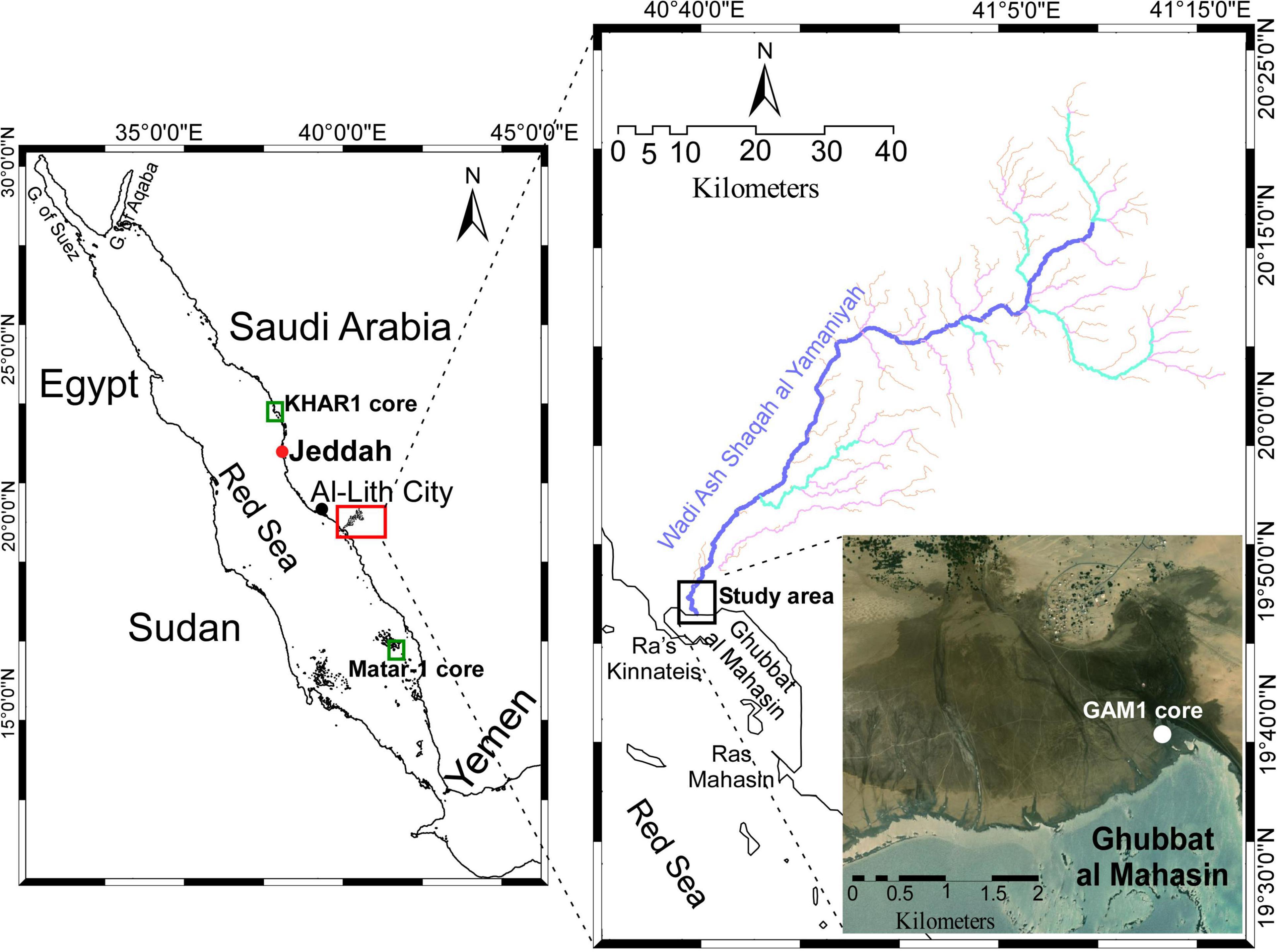
Figure 1. Simplified map showing the study area’s location with drainage systems of Wadi Ash Shaqah al Yamaniyah (this work), core KHAR1 from Al-Kharrar Lagoon (Bantan et al., 2019), and core Matar-1 from Farasan Al Kabir Island (Pavlopoulos et al., 2018) (Vectors map based on Google Earth pro images and SRTM acquired via https://portal.opentopography.org/using ArcMap 10.3 software).
Regional Setting
The investigated GAM1 core is situated at latitude 19°47′59.95″N and longitude 40°43′46.70″E on the Red Sea coast, south of Al Lith City, Saudi Arabia (Figure 1). This site is accurately located in the northern Ghubbat al Mahasin, which receives a drainage system from Wadi Ash Shaqah al Yamaniyah. Ghubbat al Mahasin is a bay with an N-S axis, larger than a cove but smaller than a gulf (class H - Hydrographic) in Saudi Arabia, and is confined by two marine headlands, Ras Mohaisain in the south and Ras Kinnateis in the north (Al-Zubieri et al., 2020). Various geomorphic features currently exist in this area, such as sabkha, mangroves, and the delta plain of Wadi Ash Shaqah al Yamaniyah, that are partly altered by land use. The area surrounding the investigation site is covered by Quaternary aeolian sand, pediment materials, and alluvial deposits (Prinz, 1983). In contrast, the catchment of the wadi extends into Proterozoic sedimentary, plutonic, and hypabyssal intrusive rocks (Figure 2).
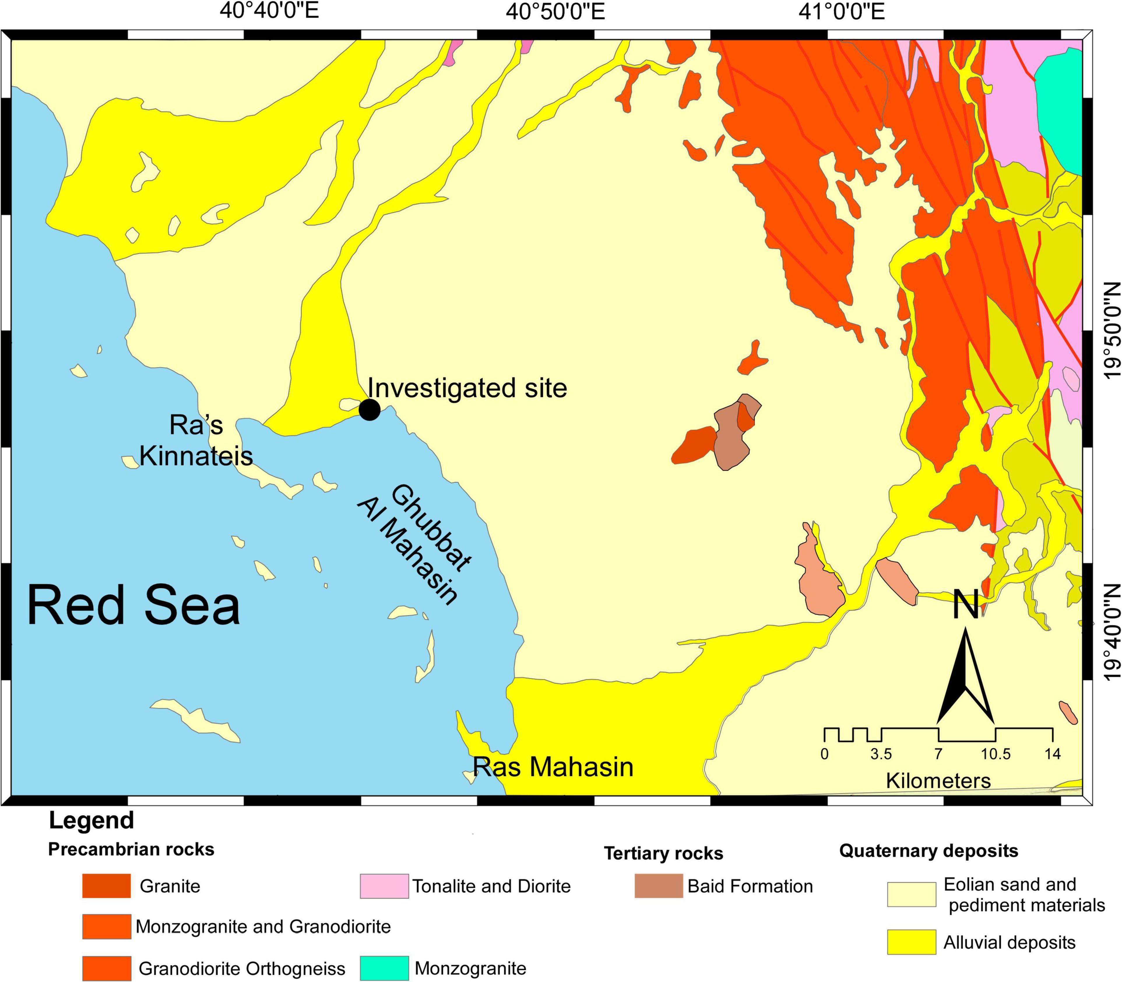
Figure 2. Geological map of the study site (modified after Prinz, 1983).
Tropical monsoons influence the recent climate of the investigated area with warm and dry conditions throughout the year, and the average temperatures range between 29 and 38.5°C in spring and 21–30°C in winter. The relative humidity is generally high throughout the year. It ranges from 18 to 86% (MAW, 2003). The mean monthly rainfall is scarce (around 63 mm per year) with intermittent wadi channel inflows. The highest significant precipitation occurs during the rainstorm time (October to March). The prevailing NNW wind blows along the Red Sea all year. However, during winter, the strong monsoon-related SSE wind passes through the Strait of Bab el Mandeb northward and converges with the prevailing NNW wind at about 19 N (Murray and Johns, 1997; Siddall et al., 2003). The Red Sea is exposed to winds flowing northwest during the summer (June to September) (Edwards, 1987; Abu-Zied and Bantan, 2015). The annual variation of the mean Red Sea tide range is 0.4–0.8 m. The velocities of both diurnal and semidiurnal tidal currents ranged from 0.1 to 1 m s–1 in 2013. This indicates the occurrence of an anticlockwise amphidromic system in this part of the Red Sea (Gharbi et al., 2018). The limited tidal range and the low tidal current velocities result in a brief flooding of the tidal flat without an incision of tidal channels (Behairy et al., 1991). The tidal velocities may surpass 1–2 m s–1 due to the shallow opening and occurrence of sand bars and low islands (Al-Zubieri et al., 2020).
Materials and Methods
This study is based on a multi-proxy approach, including geomorphological mapping, shallow subsurface sedimentary facies, benthic foraminiferal assemblages, oxygen and carbon stable isotopes, and concentrations of major and trace elements in the sediments.
Three data sources were used for geomorphological mapping and geomorphologic discrimination purposes, including Landsat 8 imagery, the digital elevation models of Shuttle Radar Topography Mission (SRTM), and a geologic map published by Prinz (1983). Digital image processing was applied to the Landsat 8 imagery (acquired in 2018) using ArcGIS 10.3 package. Principal Component Analysis (PCA), using the Crosta and Moore (1989) technique, between seven satellite image bands was conducted to discriminate the different geomorphologic features in the investigated area. The main objective of this technique is to eliminate multispectral data redundancy. It is commonly used for image processing in geology. Digitized topographic and geological maps have been used for geometric correction of satellite images. The above findings were checked, updated or completed with new data and modern sedimentary features from a field survey. A recent Google Earth satellite image was also used as a base map for modern sedimentary feature recognition (Figure 3A).
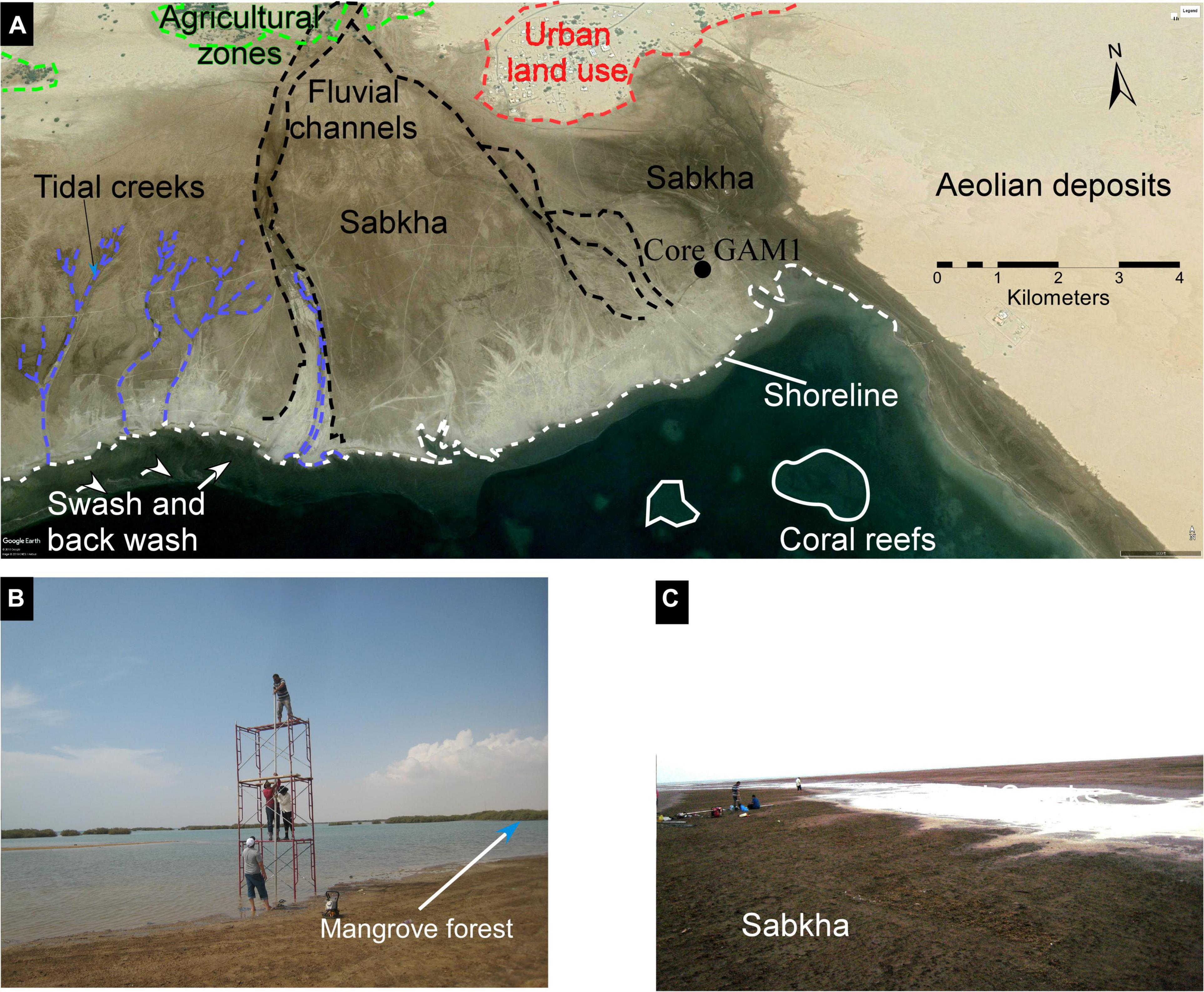
Figure 3. (A) Google Earth image showing the modern sedimentary features and shoreline configuration, (B) Field photo showing the procedure of retrieving the GAM1 core, and mangrove forest, and (C) Field photo showing sabkha, and tidal creeks in the investigated area.
A 2.84 m long sediment vibracore was retrieved from the investigated coastal site (Figure 1), using a stainless-steel tube with a 6.3 cm inner diameter. The procedure of retrieving the core is shown in Figure 3B. Its location was close to the shoreline with an elevation of 0.30 m above the present mean sea level (PMSL) to ensure the longest record produced by the high sedimentation rate. In the laboratory, the core was split lengthwise into two halves, and each half was cleaned, photographed (Figure 4), and described in terms of vertical variations in grain size, color, body, and trace fossil content and type and shape of bed contacts following the method of Ghandour et al. (2020). One half was stored as a reference, and the other half was subsampled at 2 cm intervals. The subsamples were washed through a 2 mm sieve to separate gravel size material (shell fragments) from the sand and mud fractions. Gravel size material was dried in an oven at 55°C and then visually studied to identify the type of shells that it contains. The material finer than 2 mm was air dried prior to analysis by laser diffraction using a Malvern Mastersizer 2000 at the University of Wollongong. Eighteen samples were selected to determine organic matter and carbonate contents, concentrations of major and trace elements, and micropaleontological investigation. Besides, 11 samples were selected for stable isotope (δ18O, δ13C) analyses of bulk sediments and mollusc shells.
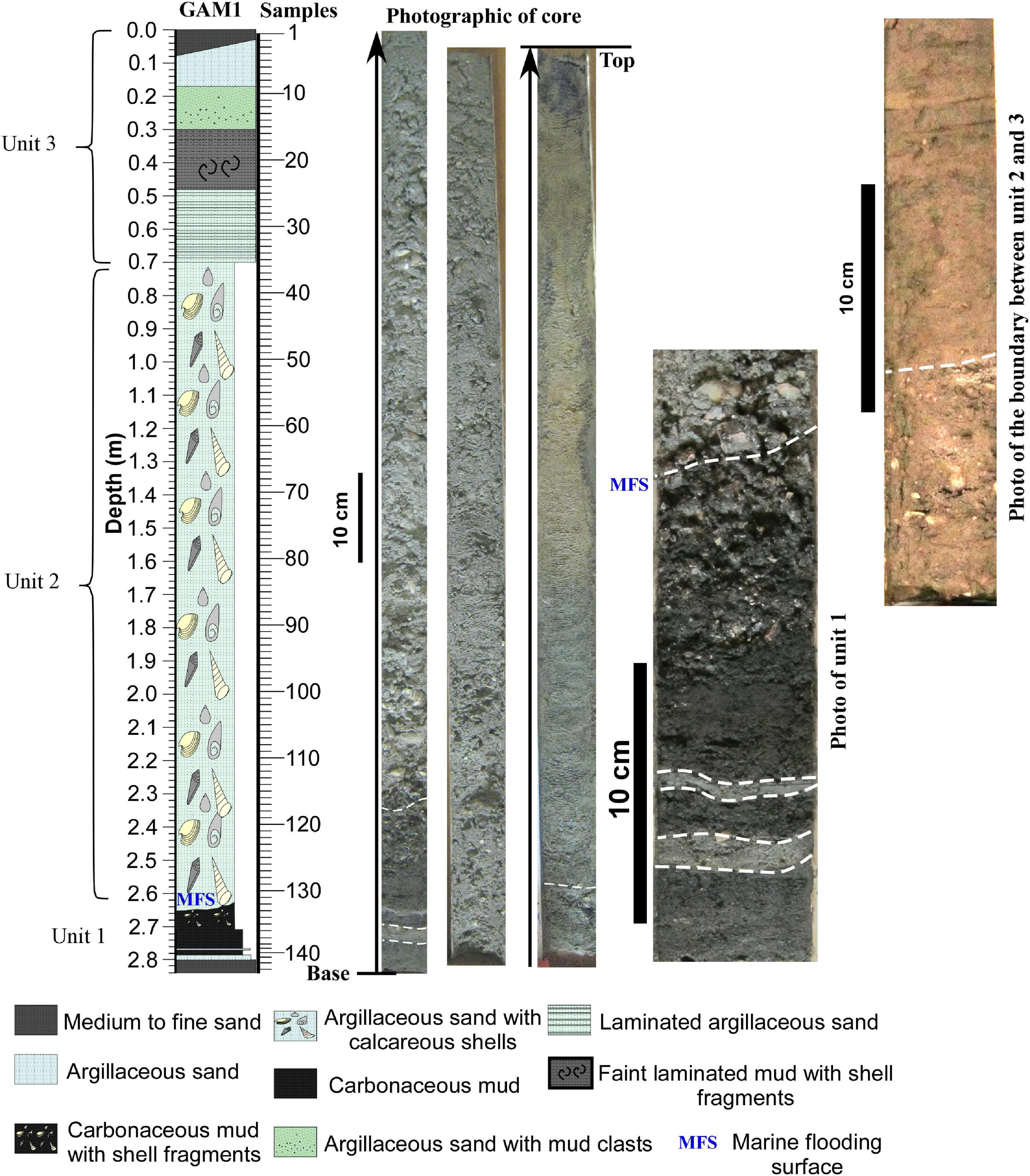
Figure 4. Lithology of the sedimentary record of the Ghubbat al Mahasin coast (GMA1), the white dotted lines indicate the boundaries between units and layers.
The CaCO3 content was determined using a Bernard Calcimeter (Lewis and McConchie, 2012). The technique involved oven-drying the sediments (for 24 h at 105°C) followed by treatment of a measured weight of sample with HCl 10% in a 20 ml bottle inside the calcimeter. The pressure reading was taken and compared with a standard curve of carbonate content, prepared by using pure CaCO3, to obtain the %CaCO3 in the sample.
Organic matter content in the selected samples was measured using the loss-on-ignition (LOI) method (Heiri et al., 2001). The technique involved oven-drying the sediments (for 24 h at 105°C), weighing the samples, then heating in a muffle furnace at 550°C, and reweighing the samples. The difference in mass before and after heating the samples was used to calculate organic matter contents. The remaining heated samples were then heated at 1000°C to remove carbonate and determine siliciclastic contents. The elemental composition for the major and trace elements was determined using an Inductively Coupled Plasma Atomic Emission Spectrophotometer (ICP/AES-Perkin Elmer 400) at the Geochemical Laboratory of King Saud University, Saudi Arabia. The method involved accurately weighing around 50 mg of the selected samples into dry and clean Teflon microwave digestion vessels, adding 2 ml of HNO3, 6 ml HCl and 2 ml HF to the vessels, following the procedure of Loring and Rantala (1992). Samples were digested using a scientific microwave (Model Milestone Ethos 1600). The resulting digest was transferred to a 25 ml plastic volumetric tube and made up to the mark using deionized water. A blank digest was carried out in the same way.
To identify the benthic foraminiferal assemblage in the selected samples, sand-mud fractions were split using a micro-splitter to reduce the amount of sediment and the number of foraminiferal species to approximately 200 individual per sample. The recovered foraminiferal species were picked and mounted on faunal slides, identified, counted, and presented as the total number of tests per gram of dry bulk sediment (hereafter called density) and percentages of the total death assemblage. Benthic foraminiferal diversity in the selected sediment samples of the core was calculated using Primer V 5″ (Clarke and Warwick, 1994). The individual foraminifers were identified following Loeblich and Tappan (1987), Abu-Zied and Hariri (2016) and Al-Dubai et al. (2017).
Stable isotopic analysis of bulk sediment samples and mollusc shells was performed in the Environmental Isotope Laboratory of the University of Arizona in Tucson, USA, using an automated carbonate preparation device (Kiel-III) coupled to a Finnigan MAT 252 mass spectrometer. The selected samples were reacted with dehydrated phosphoric acid (specific gravity = 1.92 g/cm3) under vacuum at 70°C. All δ13Ccarb and δ18Ocarb values are reported in ‰ against Vienna Pee Dee Belemnite (VPDB). The analytical precision for both δ13C and δ18O are 0.08‰ and 0.1‰ (1σ), respectively.
Four samples of clean bivalve shells were selected from the base, central portion and top of Unit 2 in the GAM1 core for AMS 14C analysis to define the age of the fossiliferous succession. The age dating was carried out at the University of Waikato Radiocarbon Dating Laboratory in New Zealand. The calibrated ages are based on OxCal v4.4.3 (Bronk Ramsey, 2021) with the marine data from Heaton et al. (2020) using the average delta R of −48.38.
Results
The results of geomorphological and sedimentological studies south of Al-Lith, Saudi Arabia, contribute to the paleoenvironmental reconstruction of the Red Sea coastal area at Ghubbat al Mahasin during mid to Late Holocene. The results are outlined and discussed in the following sections.
Geomorphological Mapping
The Crosta and Moore technique is applied in the present work on six bands (visible bands and shortwave infrared bands), taking into account only the bands that exhibit spectral features (reflectance/absorption) caused by carbonate deposits, wet sediments, plant cover, and seawater or water bodies. The resultant six principle components (PC) of the Crosta and Moore technique are illustrated in Table 1, where the first component encompasses the brightness information, sometimes called albedo. It is clear that PC1 has high positive eigenvector loadings for all bands and contains about 96.96% of the total data variation. Therefore, the results of the PCs enable discrimination of geomorphological features in the study area, carbonate deposits (e.g., coral reefs) under the seawater with a dark-green color, tidal flats with a dark red color, mangrove forest, and agricultural zones with a light-green color, sabkha deposits with a light-brown color, and the aeolian sediments have a dark-brown color (Figure 5A). This discrimination’s raster data are successfully classified using the ArcGIS package and are presented as a geomorphological map of the investigated area (Figure 5B).
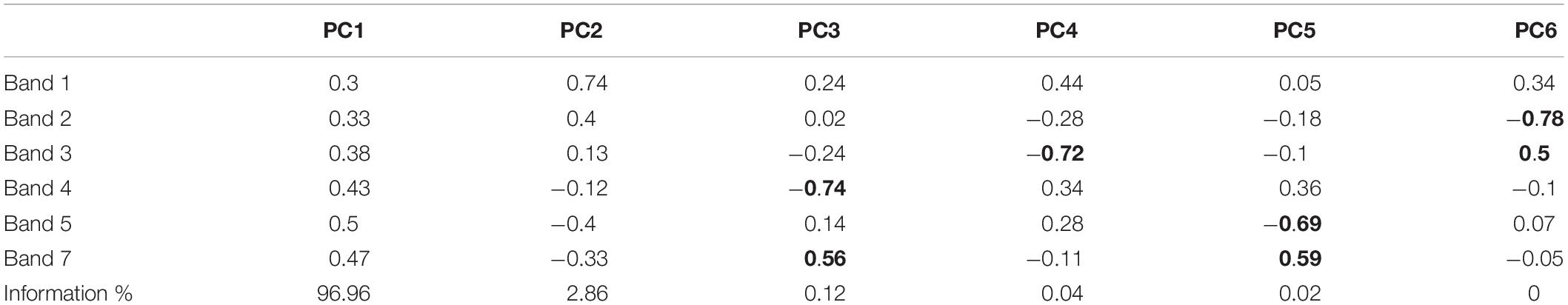
Table 1. Eigenvector loadings and eigenvalues of Crosta and Moore PCs.
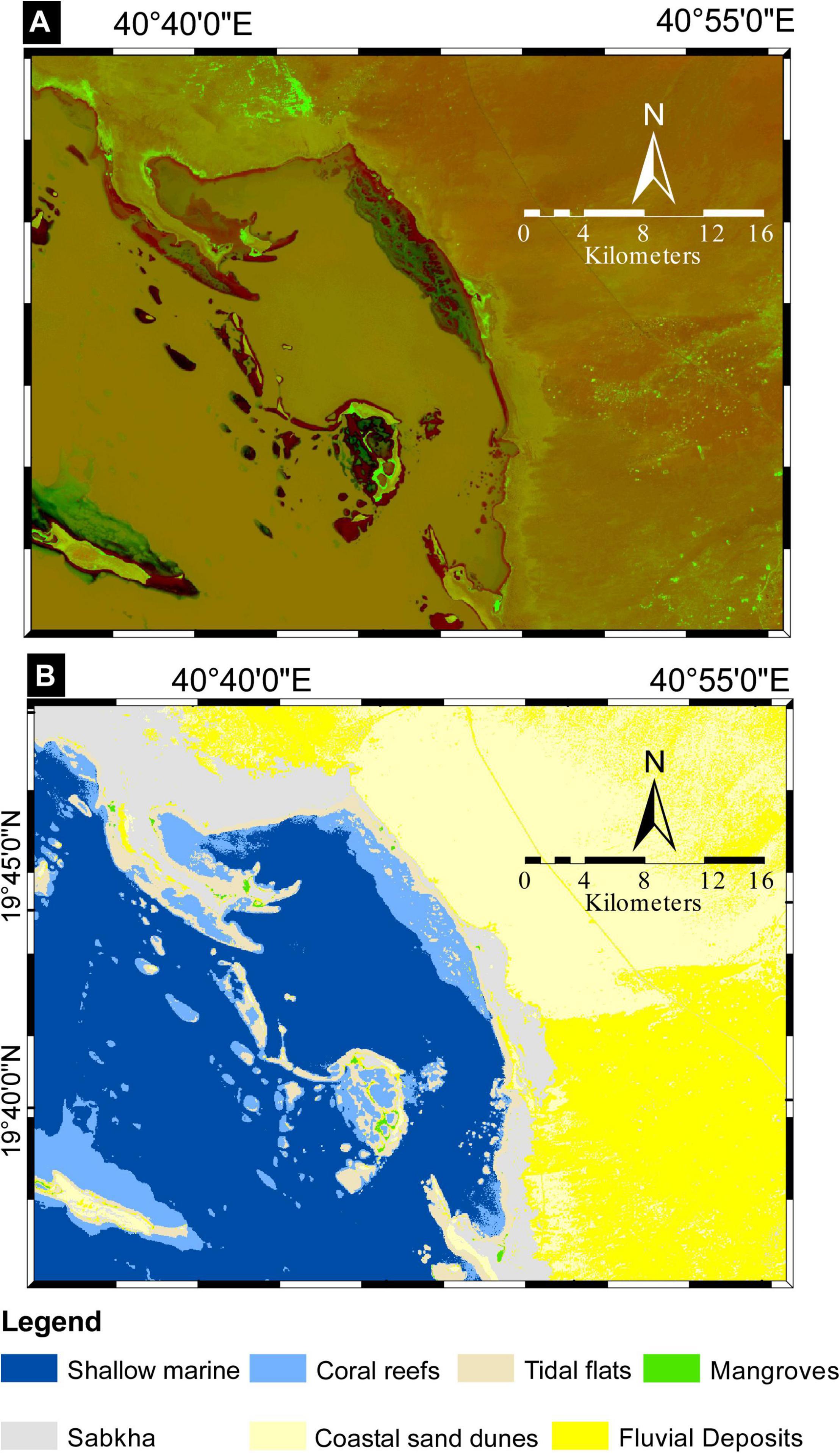
Figure 5. (A) A red-green-blue principle component analysis (RGB PCA) image (using PC3, PC5, PC6), and (B) The geomorphological map of the investigated area (The satellite images were acquired via https://eos.com/landviewer/ and were generated using ArcMap 10.3. and Canvas 12 software).
On the other hand, several modern sedimentary feature were recognized during the fieldwork, which helped update the geological mapping results. These included fluvial channels, sabkha, aeolian deposits, tidal flats, tidal creeks, and coral reefs, as well as urban land use and agricultural zones. These features are mapped using high-resolution Google Earth and are represented in Figures 3A–C.
Core Stratigraphy
The base of the 2.84 m long core ended in compact mid-Holocene strata. Based on the textural characteristics, color variation, contact surfaces, and fossil contents, three depositional units are recognized and arranged from the base of the core upwards as units 1 to 3 (Figure 4). The characteristics and interpretations of these units are described in the following sections. The summary statistics of major and trace element concentrations are shown in Tables 2, 3, respectively.
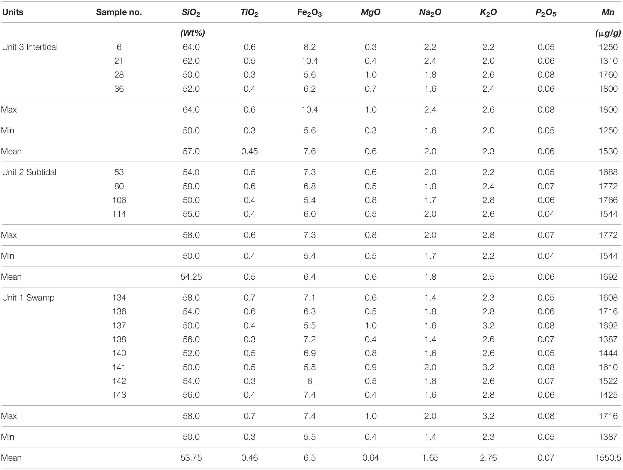
Table 2. Concentrations and summary statistics of major elements in the selected samples from core GAM1.
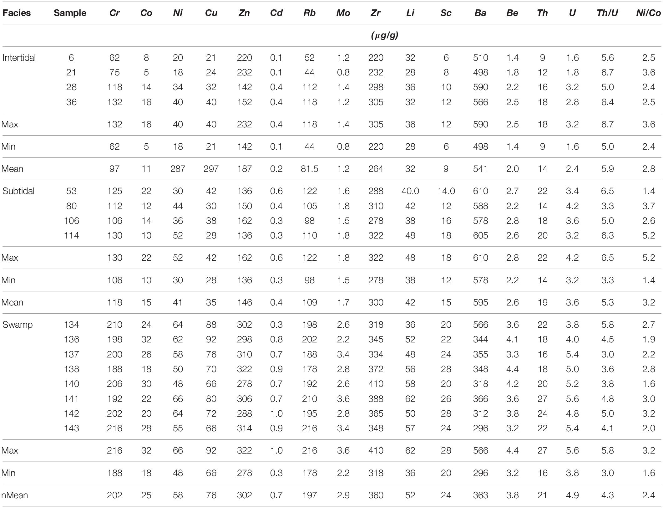
Table 3. Concentrations and summary statistics of trace elements in the selected samples from core GAM1.
Unit 1: Depth 2.84–2.64 m
This unit occupies the basal part of the core. It consists of three distinctive layers: Layer-I embraces the lowermost 4 cm, consisting of dark gray massive generally fine-grained silty sand (Figure 6) with abundant mica. It is dominated by siliciclastic materials (96.85%), a low carbonate content (2.15%), and organic matter (OM, 2.45%). Shell fragments and microfossils are undetectable to absent in this layer, and it has a sharp and possibly slightly erosive contact with the overlying layer-II (Figures 4, 7).
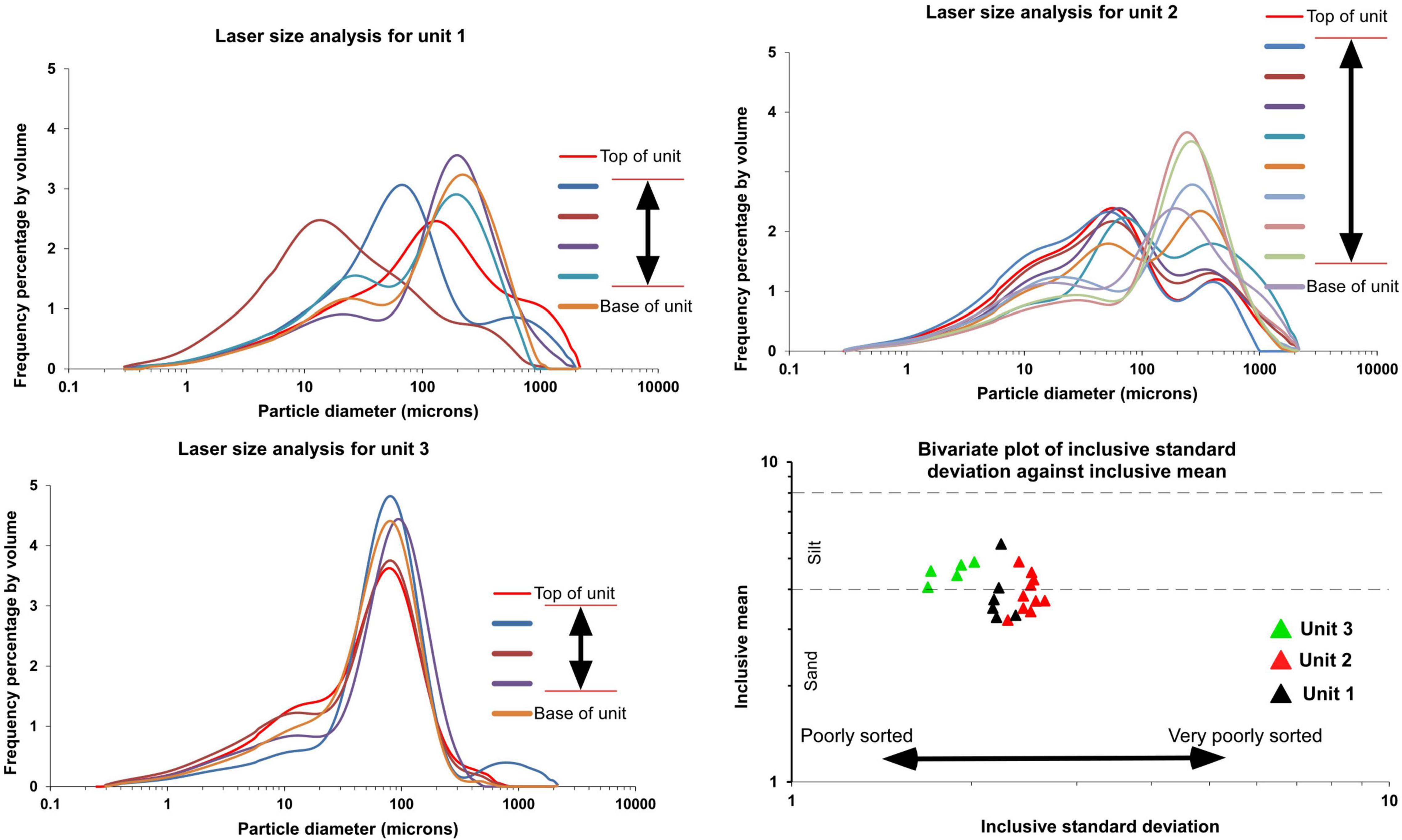
Figure 6. Grain size analysis plots for Units 1 to 3 showing two prominent modal sizes – a silt-very fine sand mode (50–77 μm) and a fine to medium sand mode (200–415 μm). Unit 3 is poorly sorted, whereas Units 1 and 2 are very poorly sorted.
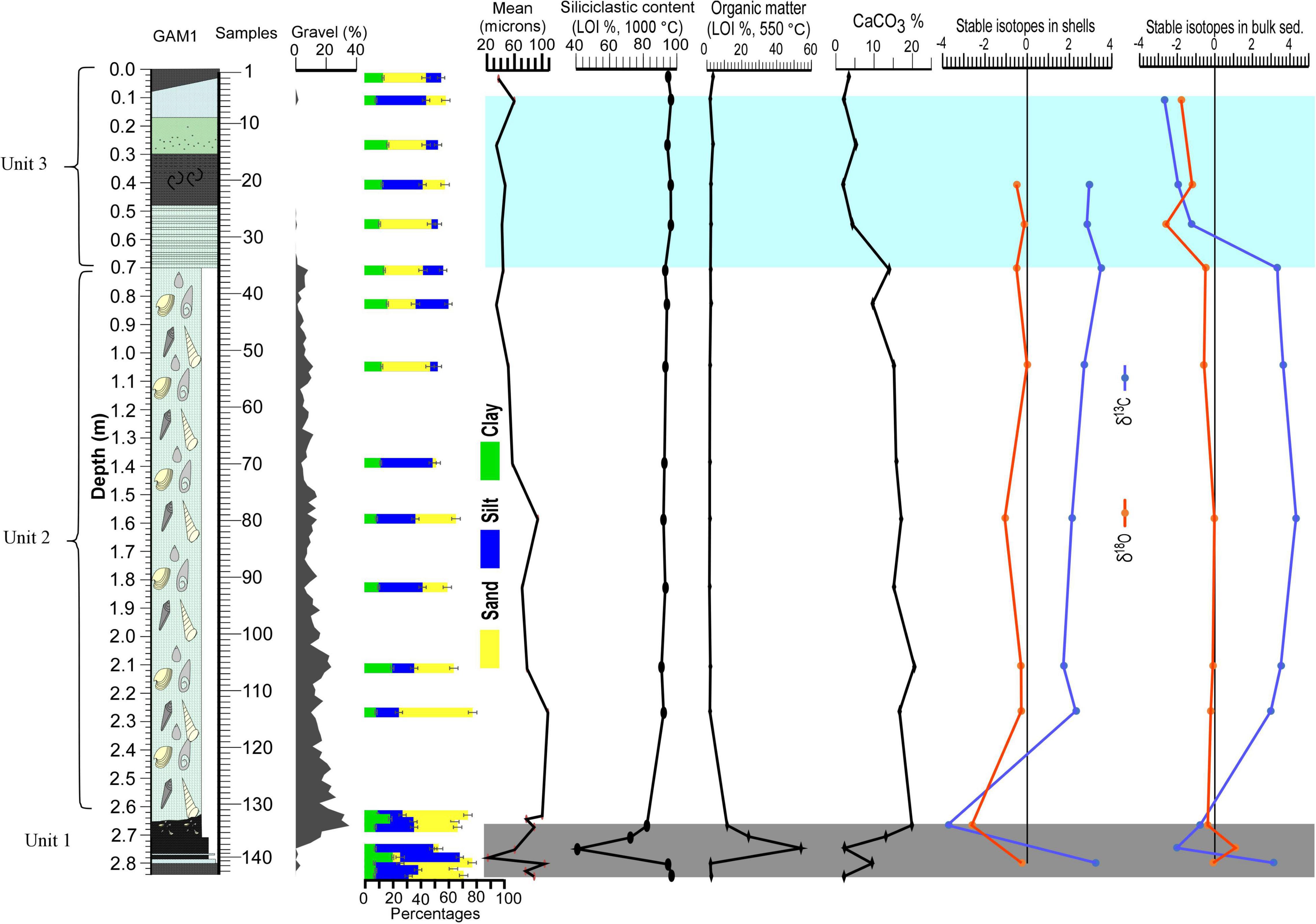
Figure 7. Vertical variation of granulometric, siliciclastic, carbonate content, organic matter (LOI), and stable isotopes in bulk sediments and shells.
Layer-II appears as two thin beds (1 and 0.5 cm thick) of argillaceous sand with rare microfossils (Quinqueloculina limbata and Triloculina trigonella; Figure 8). It is marked by a distinctive gray to brownish-gray color and alternates with layer-III. OM in layer-II is also rare, but carbonate content increased slightly to 9.45% (Figure 7). Carbon isotopes in shells and bulk sediments from layer-II are 3.25 and 3.13‰, respectively, while the corresponding δ18O are −0.25 and −0.09‰, respectively.
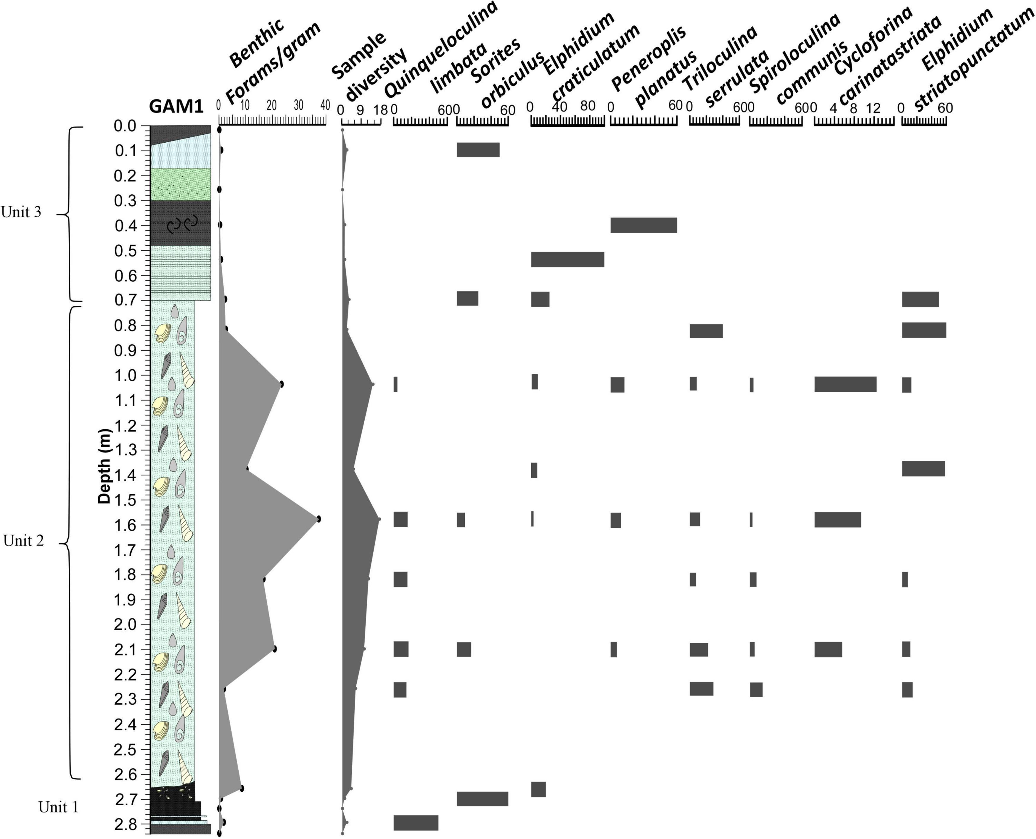
Figure 8. Relative abundances of the critical benthic foraminiferal species in the core GAM1.
Layer-III appears as two very carbonaceous mud beds with thicknesses 2 and 12.5 cm at depths 2.79-2.77 and 2.775-2.64 m. They are black to dark brown in color, compact and consist of well-humified deposits with some woody detritus. Layer-III is highly enriched in OM (up to 53.6%), while the average carbonate content is 2.28%. Carbon and oxygen isotopes of bulk sediments are −2.02 and 1.10‰, respectively. Layer-III is characterized by the relative enrichment of δ18O (positive value) compared to the other layers and units that have negative values (Figure 7). On the other hand, siliciclastic contents varied from 40.8 to 82.1%, with a mean of 65.1% (Figure 7). Layers with low siliciclastic contents have a peat-like appearance. Major and trace elements in this unit are slightly shifted compared to other units and fluctuate throughout the layers (Figures 9A,B). For example, the concentration of TiO2 varies between 0.3 and 0.7%, and the minimum value is recorded in layer III (Table 2). This unit is also characterized by the maximum values of most trace elements (for more details, see Figure 9B and Table 3). The top of the thicker bed is represented by reworked sediment mixed with shell fragments and is contacted sharply by an irregular marine flooding surface (Figure 4) with the overlying unit.
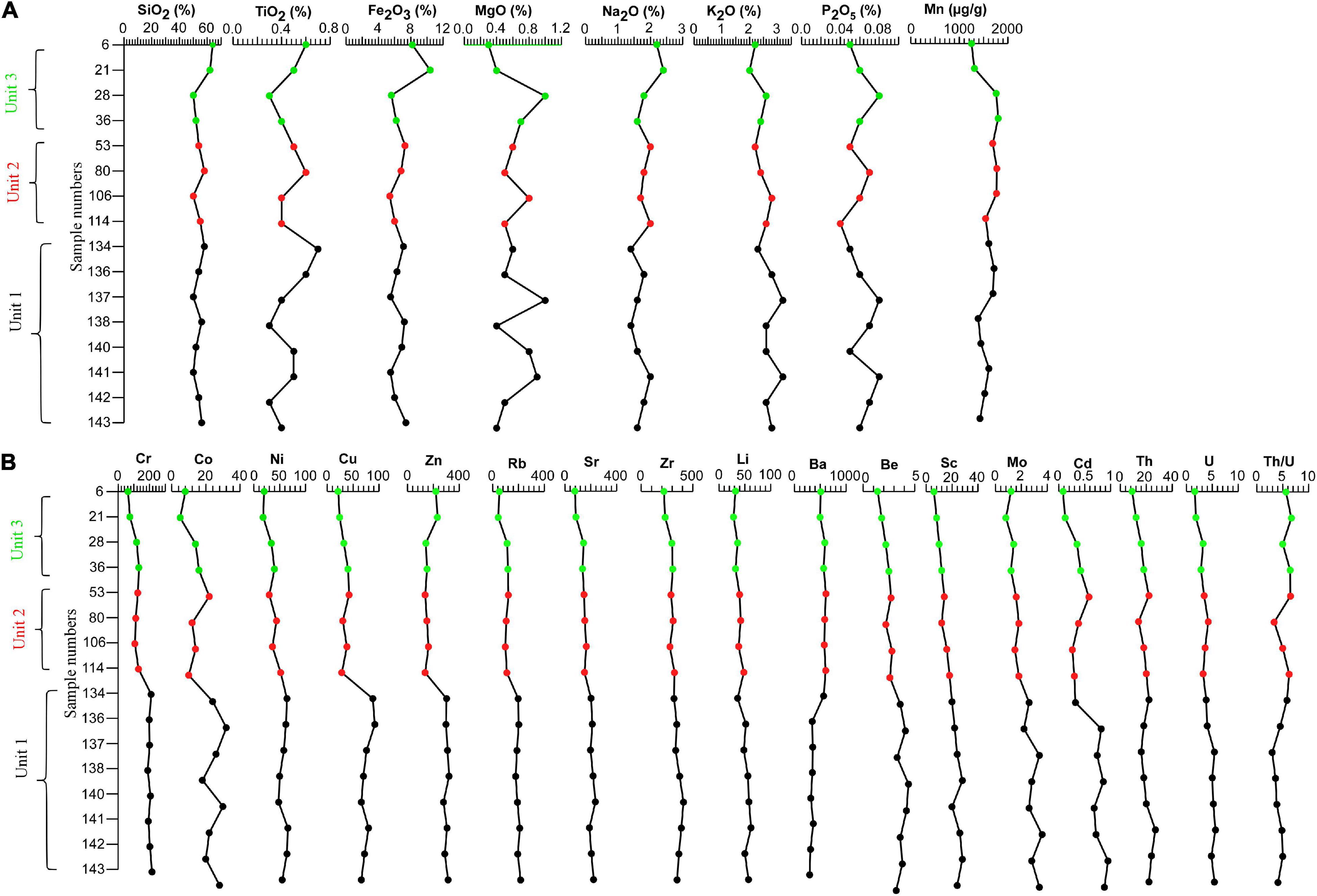
Figure 9. (A) Vertical variation of the major elements concentration in the core GAM1, and (B) Vertical variation of the concentration of minor elements (μg/g) in the core GAM1.
The clastic beds in Unit 1 have the greatest range of modal grain sizes from fine silt to fine sand, and all the samples are very poorly sorted with moderate clay contents (Figure 6). Sample 138 is a very fine sand, but it has a coarse-grained second mode that consists mainly of organic fragments. Some samples have too much organic matter, even after treatment with hydrogen peroxide, to consider conducting a meaningful grain size analysis.
Unit 1 Interpretation
The massive medium- to fine-grained sediments with abundant mica and sparse carbonate content at the base of the core suggests the dominance of terrestrial sediments, which probably accumulated during wadi floods in a relatively moderate to low energy environment. Similar features of deposits are recorded in several coastal sedimentary cores (Boski et al., 2015; Kumar et al., 2018) and are interpreted as representing a fluvial depositional environment. Likewise, the dominance of terrestrial sediments at the base of sedimentary cores retrieved from intertidal deposits in Al-Kharar Lagoon are explained by Bantan et al. (2019) and Ghandour and Haredy (2019) as an increased influx of terrestrial sediments. The thin layers of gray to brownish-gray argillaceous sand indicate a transition of depositional conditions to a supratidal under the initial influence of rising sea level on the very low gradient topography. This is supported by a slight increase in carbonate content and the appearance of foraminiferal species (such as Quinqueloculina limbata and Elphidium craticulatum) that were emplaced by post-mortem transport during high spring tides or by sea breezes.
The carbonaceous mud beds suggest a swamp or saltmarsh environment occurred during humid periods, which could coincide with the mid-Holocene warm conditions. According to Wang et al. (2013, 2018) and Song et al. (2019), carbonaceous mud beds form in the range of mean spring high water (MSHW) to mean high water (MHW), or they may occur in a saltmarsh or swamp environment where continuous high water levels led to the preservation of organic matter. The enrichment of organic matter (up to 53.6%) indicates dysoxic conditions as supported by the decrease in the Th/U ratio, which reaches around 3 (Figure 9B). Dypvik and Harris (2001) and Tribovillard et al. (2006) mentioned that a decrease in Th/U is a good indicator of dysoxic conditions in the environment and is associated with the enrichment of organic matter in the depositional environment. On the other hand, the increase of δ18O to positive values reflects a warm climatic condition in or around the region (Felis et al., 2000; Abu-Zied and Bantan, 2015; Tiwari et al., 2015; Steinman et al., 2016; Val et al., 2017). The abundant epiphytic foraminiferal species (Sorites orbiculus, which represents a typical intertidal species) at the top of the layer indicates the prevalence of seagrass meadows that is consistent with the warm climate (Abu-Zied and Bantan, 2013; Bantan et al., 2019). Altaba (2013) stated that the increase in seaweed habitats in North Africa, especially near the coasts of Libya and Tunisia, was also associated with the presence of warmer water due to climate warming. The marine flooding surface at the top of this unit indicates a relative sea-level rise or shoreward marine erosion, which occurred at 6000 year BP.
Unit 1 is interpreted to have started with increased fluvial sediment influx during the warm and humid mid-Holocene climate, and converted subsequently to a terrestrial/swamp due to sea level rise (deMenocal et al., 2000).
Unit 2: Depth 2.64-0.72 m
This unit is 1.92 m thick, contacting sharply with the underlying unit along an irregular surface overlain by large bivalve and gastropod shell fragments. It comprises light gray silty medium-grained sand in the lower 1.5 m and sandy coarse silt in the top 0.4 m (Figure 6). The unit contains abundant calcareous shells and shell fragments, mostly gastropods and bivalves, and rare coral reef fragments. This unit may be correlated with the basal unit in the cores collected from the intertidal zone of the Farasan Island (Pavlopoulos et al., 2018) and the northern Al-Kharrar Lagoon (Bantan et al., 2019). The content of shell fragments and mean grain size decrease gradually upwards (Figure 7). The abundance of microfossils is generally low, but included Elphidium craticulatum, Masslina gualtieriana, Peneroplis planatus, Pseudomassilina reticulata, Q. bicarinata, Q. costata, Q. limbata, S. orbiculus, Spiroloculina communis, T. serrulata, and Vertebralina striata. The diversity and abundance of the main species are presented in Figure 8. The OM content in unit II fluctuates between 1.75 and 2.4%, while carbonate content varies between 9.63 and 20.48%. The content of siliciclastic materials increases gradually upward (Figure 7). The δ13C values in bulk sediments and shells fluctuate between 1.73‰ and 4.32‰, while the δ18O values in bulk sediments range between −0.10 and −0.59‰ and in shells varies from −2.60‰ at the base to −0.02‰ near the top (Figure 7). The vertical profiles of major and trace elements are homogenous with slight upward increase in their concentrations (Figures 9A,B).
Unit 2 Interpretation
According to the lithologic variations, this unit is interpreted as subtidal facies within the bay environment of Ghubbat al Mahasin. The base of this unit is interpreted as transgressive flooding surface defined by concentration of mollusca shell fragments. The basal part of this unit is characterized by the appearance of shallow subtidal benthic foraminiferal species (E. striatopunctatum, Cycloforina carinatastriata, and T. serrulata). The remainder of the unit probably accumulated under shallow subtidal conditions within a protected bay environment. The upward decrease of shell fragments and the fluctuation of carbonate content and abundance and diversity of benthic foraminifera suggest mutable environmental conditions associated with shallowing and fluctuations in terrestrial material input from the wadi. The enrichment of δ13C suggests relatively high phytoplankton productivity in the Red Sea evaporative basin, where degassing of carbon dioxide from the water causes the concentration of aqueous 13C (Abu-Zied and Bantan, 2015). The enrichment of δ13C in the ancient subtidal sediments and shells is interpreted as enhanced 13C uptake during carbonate production under drier conditions (Coimbra et al., 2016). The negative δ18O values in the shells and bulk sediments indicate increased aridity and evaporation rates through the unit. The highly negative δ18O value (−2.60‰) in shells at the base of unit 2 could be related to the effect of sea level rise, where the δ16O-rich water entered through the Strait of Bab-el-Mandeb toward the central Red Sea as the post-glacial sea level rose. The fluctuations of major and trace elements could be attributed to the vertical variation of siliciclastic material input and grain size properties. The slight upward decrease in some trace element concentrations can be attributed to variation in mineralogical composition rather than grain size.
Unit 3: Depth 0.72-0 m
This unit occupies the uppermost part of the core with a thickness of 0.72 m. Generally, this unit consists of four stacked argillaceous, very fine-grained sand beds, which are characteristically distinguished by their light gray to greenish-gray colors. Unit 3 has a sharp basal contact with the underlying unit and possibly corresponds to units 3 and 4 at the top of the core studied by Pavlopoulos et al. (2018). This unit’s basal bed comprises parallel laminated argillaceous very fine to fine sand with a low diversity of foraminifera consisting mainly of E. craticulatum and E. striatopunctatum. The E. craticulatum reaches a maximum relative abundance in this bed (Figure 8). The contact with the overlying bed is gradual, and it comprises argillaceous, very fine sand and mud layers, a few millimeters thick at the top with a low diversity of foraminifera consisting mainly of the epiphytic species P. planatus. The third bed occupies the middle of the unit, consisting of greenish mud with some sand-sized clastic material and contacting sharply with the upper bed. The unit’s uppermost bed consists of light gray massive argillaceous, very fine sand capped by dark brown massive argillaceous, very fine sand layers. It is characterized by the absence of shell fragments and low diversity of foraminifers, including Cibicides cf. C. pseudolobatulus and the symbiotic species S. orbiculus. The carbonate content and OM of this unit range from 1.94 to 5.26% and 1.85 to 3.45%, respectively. Both δ13C and δ18O of shells in this unit show only slight changes, whereas δ13C and δ18O of the bulk sediments dramatically decreased to a minimum negative value (−2.6‰) (Figure 7).
On the other hand, the relative abundance of siliciclastic content in this unit reaches maximum values, which range from 94.4 to 96.5% (Figure 7). The concentrations of both major and trace elements show slight shifts compared to the underlying unit (Figures 9A,B). It is characterized by the minimum values of Mo (1.4-0.8, mean 1.2 μg/g), Li (36.0-28.0, mean 32.0 μg/g), Sc (12.0-6.0, mean 9.0 μg/g), Th (18.0-9.0, mean 13.8 μg/g), and U (3.2-1.6, mean 2.4 μg/g; for more details see Table 3). The decrease in Mg, Ba, and Sr probably reflects the much lower carbonate content toward the top of the core. The increase in Fe probably reflects the more oxidizing conditions toward the top of the core. The increased zinc content near the top of the core may indicate derivation from the urban development in the catchment.
Unit 3 Interpretation
This unit’s basal beds are interpreted as an intertidal flat deposits due to the presence of fine lamination and an increase in the epiphytic E. craticulatum and P. planatus. These species are most common in intertidal environments and may be used to indicate arid climate (Abu-Zied and Hariri, 2016; Al-Dubai et al., 2017; Cosentino et al., 2017). The stacking pattern of sedimentary beds shows the progradation of of intertidal to supratidal/sabkha deposits as the Wadi Ash Shaqah al Yamaniyah delta as sea level fell during the Late Holocene. Similar prograding systems were recorded in the sedimentary records of Al-Kharrar Lagoon coastal sediments by Ghandour and Haredy (2019). The decrease of carbonate and increase of siliciclastic materials indicate the influence of the terrestrial sediment influx. The remarkable variation in color from gray to greenish-gray and dark brown in this unit is possibly related to fluctuations in the oxygen level and the organic matter content. This explanation is also supported by the fluctuations of trace elements (Figure 9B), with minimum or high values of some elements (Table 3). The depletion of both δ13C and δ18O in the bulk sediment indicates more aridity during the deposition of this unit (Figure 7).
Chronology
The 14C dating results (Table 4) indicate that the marine flooding surface at the base of unit 2 occurred at 6010 cal.year BP initiating subtidal deposition. The remaining ages indicate that subtidal sedimentation in Unit 2 occurred fairly uniformly at sedimentation rates of 0.8-1.2 mm/year, decreasing to 0.3 mm/ year in the top 0.22 m of Unit 2. The date of 3690 cal.year BP at the top of Unit 2 records continued subtidal sedimentation prior to the subsequent progradation of the alluvial fan of Wadi Ash Shaqah al Yamaniyah.
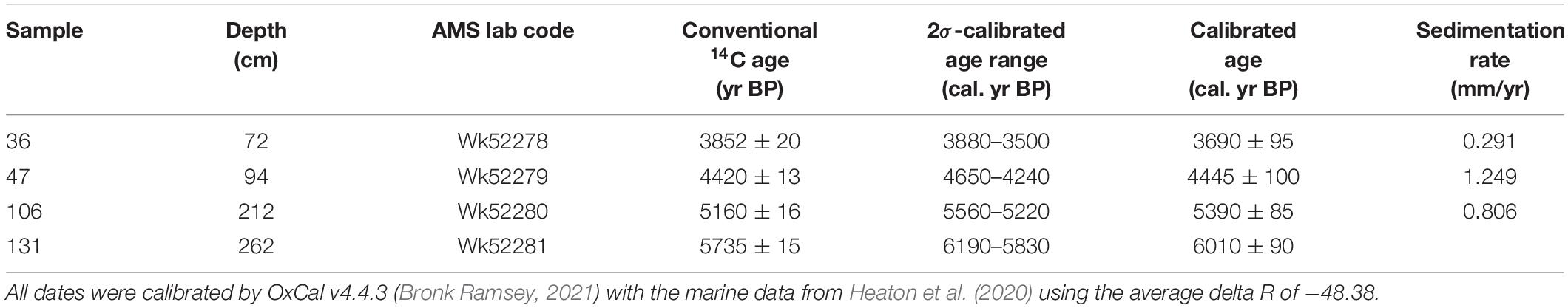
Table 4. AMS 14C dating in the GAM1 core, Ghubbat al Mahasin, central coast of the Red Sea.
Discussion
This research reconstructs the Mid to Late Holocene paleoenvironment of the Red Sea coastal zone south of Al-Lith, Saudi Arabia, using a multi-proxy approach including geomorphological mapping, sedimentary facies, benthic foraminiferal assemblages and geochemical data. It focuses precisely on the northern coast of Ghubbat al Mahasin but integrates these findings with other cores from the Red Sea coast to indicate broader sea level and climatic changes.
Modern Geomorphic Features
Geomorphological mapping based on remote sensing data and fieldwork reveals that Ghubbat al Mahasin substrata are covered by a series of coral reefs parallel to the shoreline and a narrow tidal flat along the coast. The current geomorphological features extending along the delta plain of Wadi Ash Shaqah al Yamaniyah suggest increased aridity since the late mid-Holocene. These features include fluvial channels, sabkha, aeolian dunes, tidal flats, and tidal creeks. These features have been detected at different sites along the Red Sea coast (Gheith et al., 2005; Alharbi et al., 2011, 2016; Basyoni and Aref, 2015; Rasul, 2015; Nofal and Abboud, 2016; Nabhan and Yang, 2018), and are most common on the arid parts of the coast (Johnson, 1982; Semeniuk, 1996). Fluvial channels were probably active during sporadic flash flood events from Wadi Ash Shaqah al Yamaniyah and migrated and avulsed laterally over time. Sabkha occurs in low-lying areas landward from the coast. It is probably formed due to the inundation of low-lying areas in the supratidal zone during spring tides and storm surges, and salt precipitation from moisture during the daily evaporative pumping of groundwater. It is characterized by many tidal creeks generated by tidal processes during spring and neap tides, as well as water movement caused by strong onshore sea breezes. Coastal sand dunes have formed parallel to the coast, with altitudes of 1-5 m above mean sea level. The orientation of these dunes reveals the effect of seasonal wind field shifts from onshore during winter to shore parallel approach angles in summer (Abu-Zied and Bantan, 2015).
Chronostratigraphic Framework
The sedimentary record in GAM1 can be correlated with previous works carried out in different sites on the Red Sea coast. The sedimentary records retrieved from the southeastern Farasan Al-Kabir Island coast (Matar-1 core, Pavlopoulos et al., 2018), and the KHAR1 core (Bantan et al., 2019) from the northern Al-Kharrar Lagoon coast were used for comparison. The locations of these cores are mapped in Figure 1, and the correlation framework is presented in Figure 10. The 14C dates from GAM1 confirmed that the successions for over 750 km along the Saudi Arabian coast could be directly correlated and show consistent facies relationships that are controlled by sea level.
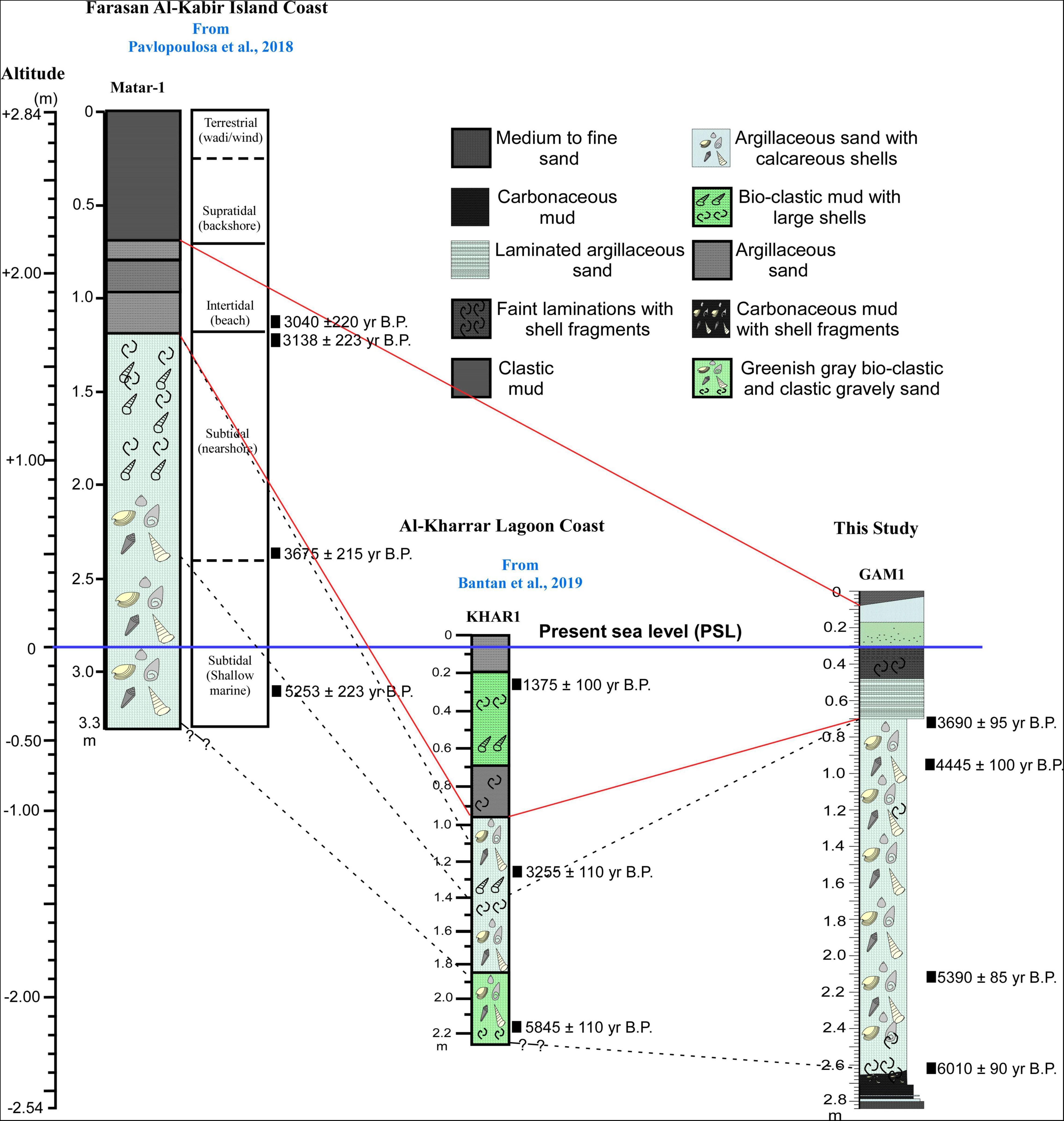
Figure 10. Chronostratigraphic correlation of the GAM1 core from the Ghubbat al Mahasin coast in the study area with the Matar-1 core (Pavlopoulos et al., 2018) from the end of Wadi Matar on the southeastern Farasan Al-Kabir Island coast and the KHAR1 core (Bantan et al., 2019) from the Al-Kharrar Lagoon on the Red Sea Saudi coast, the red lines indicate facies correlation and the dashed black lines reveal time correlation.
Based on the chronostratigraphic evidence (Figure 10), as well as characteristics of the sedimentary facies and paleoenvironmental reconstruction, the investigated sedimentary record covers the mid to Late Holocene. In GAM1 the initial swamp deposits accumulated during a period of low terrestrial input. The overlying shallow marine deposits started as the marine flooding surface crossed the site of deposition, producing a sub-tidal environment at 6000 year BP. Marine sediment accumulation ended at 3700 year BP. with later accumulation of prograding intertidal deposits and, finally, supratidal sabkha (Figures 11A–C). Pavlopoulos et al. (2018) demonstrated that the mid to Late Holocene sedimentary records at the end of Wadi Matar (Matar-1, Figure 10) on the southeastern Farasan Al-Kabir Island coast, Saudi Arabia, are organized in five sedimentary facies progressing from subtidal (shallow marine) to terrestrial (wadi/wind). Nabhan (2015) stated that the coastal deposits on the Al Qahmah coast, southern Red Sea, Saudi Arabia, prograded as two associated facies that included a shallow marine facies at the base overlain by marginal marine and non-marine coastal deposits (siliciclastic deposits). Bantan et al. (2019) recorded the dominance of lithogenous sediments at the base of the KHAR1 core before 5800 year BP, overlain at about 5000 year BP by subtidal and intertidal deposits accompanied by an increased benthic foraminiferal assemblage. In addition, gravel-rich fluvial sediments were sharply overlain by lagoonal deposits on the eastern Al-Kharrar Lagoon coast (Behairy et al., 1991).
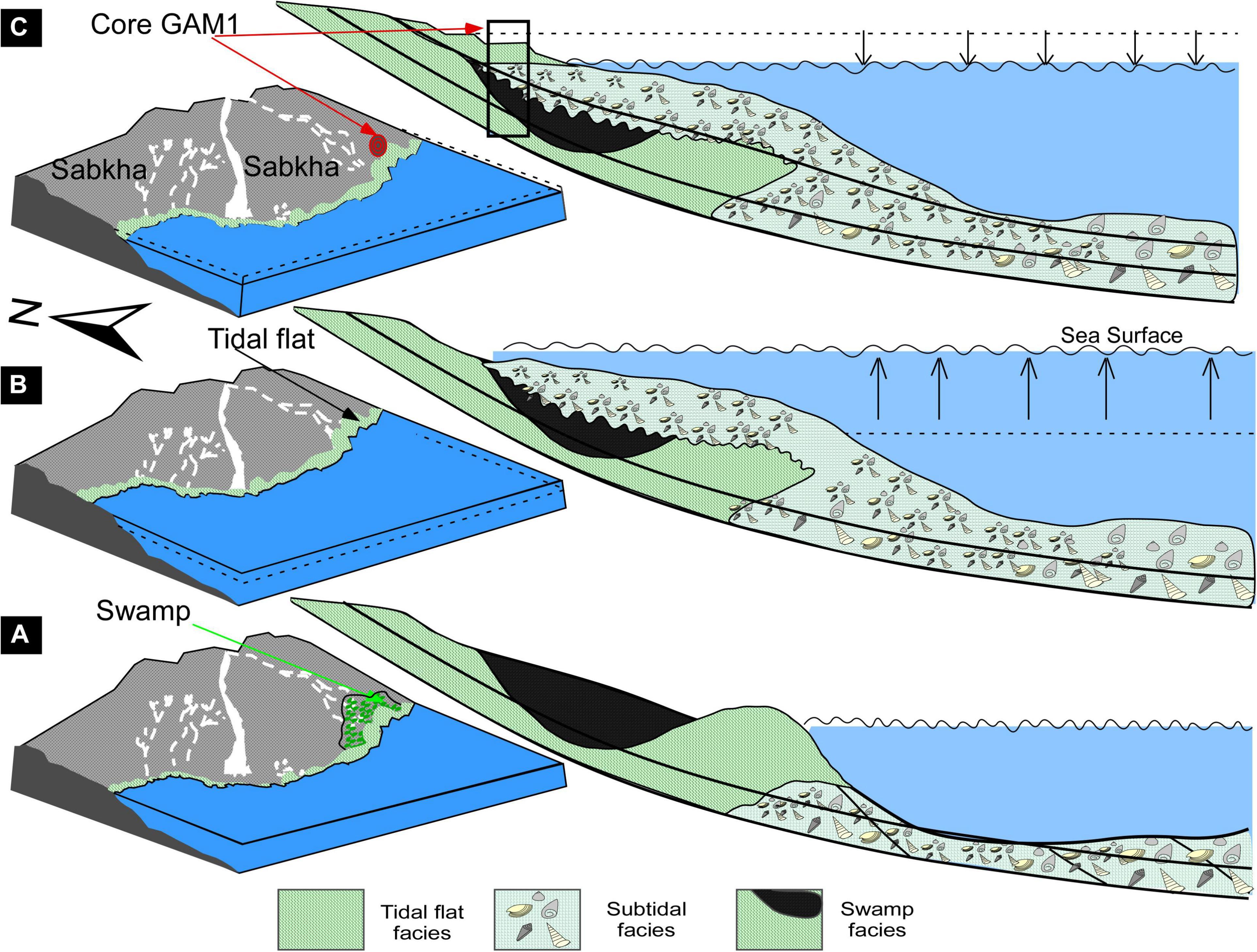
Figure 11. Schematic block diagrams displaying the paleoenvironmental evolution and stacking pattern of facies in the investigated site related to sea-level changes. (A) Early-stage terrestrial/swamp facies are deposited. (B) They are inundated by a relative sea-level rise during the mid-Holocene highstand, and (C) followed by progradation of the coastal system during the Late Holocene sea-level fall.
According to the discussion above, the Red Sea’s coastal deposits record the rise of the mid-Holocene post-glacial sea level toward the highstand at about 5000 year BP and since about 3000 year BP the Late Holocene sea-level fall probably led to the progradation of coastal systems.
Paleoclimatic Implications
The early to mid-Holocene African Humid Period (deMenocal et al., 2000; Arz et al., 2003) led to increased sediment input into coastal systems as a result of the increased fluvial activity. This accounts for the coarser sediment and minor gravel (<25%) recorded in the lower portions of the three cores shown in Figure 10. Additional evidence of the more humid conditions prior to 5-6 ka (Parker et al., 2006) is the preservation of organic-rich peat deposits in Unit 1 in the GAM1 core from the Ghubbat al Mahasin coast. The end of the African Humid Period at about 6-5 ka (deMenocal et al., 2000) led to the current arid conditions along the Red Sea coast since the mid Holocene. The increased aridity was caused by the insolation-forced gradual decline in the strength of the Indian SW Monsoon (Trommer et al., 2010). This is reflected in the slow rate of sediment accumulation because the low precipitation and high evaporation along the Saudi coast mean that sediment supply from wadis was low and infrequent. Although the shallow marine succession in GAM1 does not provide any direct climatic information, the overlying intertidal and sabkha deposits confirm the drying out and subsequent arid climatic conditions. The arid conditions are supported by the depletion of δ18O and δ13C in the bulk sediments in Unit 3 (Figure 7), as well as the presence of modern sabkha deposits.
Sea Level Implications
The central and southern Saudi coast has been tectonically stable during the Holocene (Manaa et al., 2016) and changes in accommodation space reflect eustatic changes in sea level (Ghandour and Haredy, 2019; Bantan et al., 2020; Ghandour et al., 2020). These changes vary along the Red Sea coast in the timing and the spatial distribution (Al-Mikhlafi et al., 2021). Although the GAM1 core cannot indicate the maximum extent of the post-glacial Holocene transgression it does indicate that the sea had reached 2.3 m below present sea level by 6000 cal.year BP where it overlies swamp deposits. The presence of coarse clasts near the base of the KHAR1 core at a similar time also indicate fairly shallow water higher energy conditions at 2.20 m below present sea level during this time period. However the marine transgression was recorded at about 7200 cal.year BP at −2.4 m in the ancient Egyptian harbor of Mersa/Wadi Gawasis on the western Red Sea coast (Hein et al., 2011). The erosional contact at the base of the marine sequence in the GAM1 core could indicate progressive shoreline erosion during the early phase of the transgression that did not reach the GAM1 area until 6000 year BP. The base of the Matar-1 core was still in the shallow subtidal facies at −0.46 m at about 5200 cal.year BP (Pavlopoulos et al., 2018) so provides no information about when sea level inundated the Farasan Island area.
Sea level rose to a highstand of 0.5-2 m above present sea level at about 5 ka (Hein et al., 2011). In the Gulf of Aqaba the sea-level curve shows a highstand at 6.5–4.5 ka, followed by a fall to the present-day (Shaked et al., 2002). Wave-cut notches and a coral terrace at Mersa/Wadi Gawasis indicate a highstand at 1.1-1.8 m above MSL (Hein et al., 2011). This corresponds with the wave-cut notches and aragonite cementation at similar elevations (1-1.4 m above MSL) along the Saudi coast and Farasan Islands (Manaa, 2016; Manaa et al., 2016). A coral terrace at Mersa/Wadi Gawasis was dated to 4359 ± 85 cal.year BP indicating that sea level elevation was still at least 1.1 m above MSL at this time. The relative sea level fall during the late Holocene toward current sea level, caused by isostatic processes, led to shoreline progradation from about 4000 cal.year BP (Hein et al., 2011). A similar feature was seen in the Dumaygh Lagoon north of Al-Wajh, Saudi Arabia, where the vertical stacking of intertidal and supratidal facies above a shallow subtidal facies reflects a progradational sequence that may relate to the late Holocene relative sea level fall (Ghandour et al., 2020). These progradational sequence correspond to the progradation seen at Al Kharrar Lagoon (Bantan et al., 2019; Ghandour and Haredy, 2019) and to the occurrences of beach rock up to 1.2 m above MSL formed near Rabigh during the late Holocene phase of falling sea level (Manaa, 2016).
The elevation of the Matar-1 core from the Farasan Islands may not be entirely accurate since it was obtained by GPS. However, the change from subtidal to beach at +1.68 m may indicate the maximum elevation of the highstand sea level since it is close to the best predicted maximum Holocene sea level at 5000 cal.year BP (+1.5 m) at the Farasan Islands (Hein et al., 2011; figure DR2). This also corresponds to the occurrence of mid Holocene shell middens on the islands that are 2-3 m above present sea level and date from 6000 cal.year BP (Hausmann et al., 2019). The change to intertidal conditions occurred at 3100 cal.year BP at Matar-1, and probably represents the fall in sea level as the intertidal and supratidal successions prograded over the lagoonal sequence at this site. This is confirmed by the presence of lower elevation middens closer to the present coast dating from 2300 to 1500 cal.year BP (Hausmann et al., 2019).
The sea level pattern along the Red Sea coast of Saudi Arabia is similar to that recorded at Half Moon Bay on the Arabian Gulf coast of Saudi Arabia and around Qatar (Weijermars, 1999) where the area was inundated by sea level rise just over 6000 year BP and began to fall again with beach rock development from about 4000 year BP. A more rigorous assessment of Holocene sea level changes in eastern Saudi Arabia by Parker et al. (2020) showed that the transgression rose above mean sea level at about 7000 year BP and the mean highest high tide water level was recorded as up to 3.75 m above present sea level at 5400 year BP. The Late Holocene sea level fall in the Red Sea follows the global sea level pattern (Ramsay and Cooper, 2002; Siddall et al., 2003; Sloss et al., 2018) but differs from that in the Mediteranean Sea where sea level is continuing to rise (Barnett et al., 2020).
Paleoenvironmental Evolution
The stacking pattern of depositional units (Figures 4, 11) and other proxies showed that the investigated site has evolved since the mid Holocene. As the chronostratigraphic correlation shows (Figure 10), the studied area received an enhanced terrestrial input before 6000 year BP probably by wadi floods, as indicated by the occurrence of medium- to fine-grained sand with high siliciclastic contents and the absence of carbonate materials in a relatively moderate to low energy environment. After this initial deposition, the major wadi channel migrated laterally or avulsed westward. This channel now occurs as the modern fluvial sedimentary facies north and west of the investigated site (Figures 1, 3A). Subsequently, the site became a reducing environment, possibly a pool in the abandoned channel, which was mainly separated from the marine environment (Figure 11A). The characteristics of the carbonaceous mud layers enrichment of organic matter suggest that these sediments were deposited in a dysoxic swamp environment possibly during a period of increased precipitation (Ridgway et al., 2000; Song et al., 2018) that promoted vegetation growth. The climate was warm and humid, as indicated by the enrichment of δ18O in the organic-rich bulk sediments, which coincided with the later part of the mid-Holocene African Humid Period (deMenocal et al., 2000). This warm climate event was recorded in different sites such as the Al-Kharrar Lagoon sedimentary record (Bantan et al., 2019), speleothem records (Neff et al., 2001), and lake records in the northern and southern Sahara and the Sahelian belt areas (Gasse, 2000; Arz et al., 2003).
The swamp facies was terminated by marine flooding as sea level rose during the post-glacial marine transgression. This is indicated by the occurrence of an irregular erosion surface and the presence of large reworked shells at its top (Figure 11B). This marine flooding indicates that relative sea-level flooded the study site at 6000 year BP as it rose toward the highstand of sea-level during the mid-Holocene. This is in accord with the sea-level curve of Siddall et al. (2003) that shows sea-level continued to rise from 7000 to 5000 cal.year BP. A relative sea-level rise was also documented in the coastal system’s evolution by 7200 cal.year BP at Mersa/Wadi Gawasis on the Egyptian Red Sea coast by Hein et al. (2011). The delayed arrival of the marine incursion at GAM1 may reflect an erosional haitus.
During the period 6000 to 3700 year BP (depth 2.64 to 0.72 m), a lagoonal facies was deposited, following the marine flooding and becoming shallower upwards (prograding). This facies is characterized by shells and fragments of bivalves, gastropods, and a relative abundance of benthic foraminifera, including E. striatopunctatum, C. carinatastriata, and T. serrulata. These species indicate subtidal or lagoonal environments (Abu-Zied and Bantan, 2015; Al-Dubai et al., 2017). After sea-level reached its maximum at about 5000 year BP (Hein et al., 2011), there was an abrupt change in climatic conditions to an arid, more evaporitic climate, as indicated by the depleting of δ18O values in both bulk sediment and shells (Figure 7), and sea level started to slowly fall. During the mid to Late Holocene, abrupt climate changes (ACCs) have been recorded in the sedimentary record in the Red Sea by Arz et al. (2006), and in the Middle East coastal systems by Kaniewski et al. (2008). The upward decrease of water depth during the deposition of this facies could be related to the Late Holocene sea-level fall (Figure 11C) and correlates with the time of maximum regional aridity and evaporation (4.4–3.3 ka BP) reported in central and northern Red Sea deep-sea sedimentary records (Arz et al., 2006; Legge et al., 2006; Biton et al., 2008, 2010; Edelman-Furstenberg et al., 2009). The prevailing arid conditions are also supported by the depletion of δ18O in the bulk sediments at the top of this unit (Figure 7). Abu-Zied and Bantan (2015) attributed the decreasing δ18O values in the benthic foraminifera (E. striatopunctatum) obtained from a sedimentary core at Shuaiba Lagoon as indicating an arid condition. The top of this facies is characterized by the disappearance of some subtidal foraminiferal species and the increased relative abundance of shallow water species including S. orbiculus and E. craticulatum (Figure 8), indicating a change toward an intertidal environment and/or an increased contribution of terrestrial input.
During the last 3700 years (depth 0.72-0 m), the sedimentary sequence of the investigated GAM1 core continued to prograde and the facies gradually transitioned from a lagoonal-subtidal condition below to intertidal flat and sabkha conditions at the top, as indicated by the appearance of some species of benthic foraminifera at the base and the disappearance of others at the top. The predominant siliciclastic material is highly enriched in both major and trace elements. This could be due to a continued sea-level fall and the influence of aeolian and terrestrial input (Figure 11C). The lowermost part of unit 3 is characterized by parallel laminated argillaceous very fine to fine sand with a maximum relative abundance of E. craticulatum and the epiphytic species P. planatus, which probably preferred intertidal, warmer water, and hypersaline conditions (Almogi-Labin et al., 1992; Geslin et al., 2000). The decrease in δ18O values and the remarkable negative excursion of δ13C in the bulk sediment of Unit 3 compared to Units 1 and 2, may refer to increased aridity with the change in environmental setting from lagoonal to intertidal flat. The greenish gray bed in Unit 3 at GAM1 reflects more reducing conditions that may correspond with the “Little Ice Age” (LIA) as recorded by several authors (Driese et al., 2004; Charpentier Ljungqvist et al., 2012) in the northern hemisphere. Edelman-Furstenberg et al. (2009) documented similar events in the central Red Sea during 2000-700 year BP. The top of unit 3 represents a supratidal/sabkha environment, as indicated by the modern features that probably formed as an infilling of deltaic sediment from Wadi Ash Shaqah al Yamaniyah that was submerged during high tides. These modern sedimentary features are extensive along the study area’s coastal zone and the Red Sea coast (Rasul, 2015).
Conclusion
The mid to Late Holocene paleoenvironment at Ghubbat al Mahasin, south of Al-Lith, Saudi Arabia, were reconstructed based on the stacking of sedimentary facies, benthic foraminifera, stable δ18O and δ13C isotopes, and inorganic geochemical characteristics. Besides, remote sensing data were used to identify the distribution of modern sedimentary features. The core database, coupled with a chronostratigraphy correlation from previous work on the Red Sea coast, emphasizes the following conclusions.
• The investigation site is covered by siliciclastic deposits along the coastal zone that were deposited under the modern arid climate. This has led to the recognition of modern sedimentary features including sabkha, coastal sand dunes, fluvial channels, and tidal creeks as well as mangroves forest, agricultural areas, and urban land use patterns.
• Offshore, a series of coral reefs developed in the Red Sea where suitable substrate, depth and temperature conditions are available.
• Three depositional units in the onshore shallow subsurface sedimentary record have been recognized, suggesting three distinct depositional stages.
• The first stage includes medium- to fine-grained fluvial sand deposits overlain by black carbonaceous mud suggesting deposition in a swamp during lateral movement of the fluvial system in a warm humid period in the Early Holocene prior to 6000 year BP.
• The second unit records deposition that was initiated by a marine flooding event caused by the mid Holocene sea-level rise. It records a period of subtidal deposition between 6000 and 3700 years ago and is characterized by muddy sediments containing shells and fragments of bivalves and gastropods together with shallow marine benthic foraminiferal assemblages. The sequence shallows upwards as sea level fell in the Late Holocene.
• The upper unit sharply overlies Unit 2 and consists of yellow argillaceous fine sands with rare benthic foraminiferal assemblages of intertidal affinity. It accumulated at some time over the past 3700 years with the intertidal environment being replaced by supratidal/sabkha environments as the Wadi Ash Shaqah al Yamaniyah delta prograded. This shallowing probably corresponds to the gradual sea-level fall during the Late Holocene rather than an increase in sediment supply.
• The facies along 750 km of the Saudi Red Sea coast confirm a wetter and more humid phase during the Early to mid Holocene as swamp deposits accumulated. The decline of the Indian SW Monsoon (Trommer et al., 2010) from about 4000 year BP is reflected in a slow sedimentation rate. Increasingly arid conditions are supported by the depletion of δ18O and δ13C in the bulk sediments in GAM1 Unit 3 and the presence of modern sabkha deposits. However more continuous successions in Shuaiba and Al-Kharrar Lagoons indicate fluctuating semi-arid to arid climatic conditions during the Late Holocene.
• Precise timing of the post-glacial marine transgression along the Saudi Red Sea coast could not be determined but it had definitely reached the area by 6000 year BP. Evidence from this coast confirms that the maximum sea level of about 1.5 m occurred at about 5000 year BP and it was certainly falling from about 3000 year BP.
Data Availability Statement
The original contributions presented in the study are included in the article/supplementary material, further inquiries can be directed to the corresponding author/s.
Ethics Statement
Written informed consent was obtained from the individual(s) for the publication of any potentially identifiable images or data included in this article.
Author Contributions
IG, AA-Z, AB, and AM conceptualized, designed, and conducted the work plan. AA-Z and IG performed the data analysis, prepared the figures, and wrote the draft of manuscript. TA-D performed the microfossils analyses. BJ performed the particle size analysis, provided the radiocarbon data and analysis, and improved the quality of writing. All authors reviewed the manuscript and contributed to the article and approved the submitted article.
Funding
This research work was funded by the Institutional Fund Projects under grant no. IFPHI-194-980-2020. The authors gratefully acknowledge technical and financial support from the “Ministry of Education and King Abdulaziz University, DSR, Jeddah, Saudi Arabia.”
Conflict of Interest
The authors declare that the research was conducted in the absence of any commercial or financial relationships that could be construed as a potential conflict of interest.
Acknowledgments
The authors are thankful to Ali A. Khawfany, Mr. Osama Abid, Satria Antoni, and Bandar Al-Zahrany, for the field assistance. The authors thank Prof. Athar Khan (KAU) for his valuable reading and comments which enhanced the language of the article. The authors are very grateful to the editor and reviewers for their constructive comments and editorial handling. The authors acknowledge the GeoQuEST Research Centre, University of Wollongong, for providing radiocarbon analyses.
References
Abu-Zied, R. H., and Bantan, R. A. (2013). Hypersaline benthic foraminifera from the Shuaiba Lagoon, eastern Red Sea, Saudi Arabia: their environmental controls and usefulness in sea-level reconstruction. Mar. Micropaleontol. 103, 51–67. doi: 10.1016/j.marmicro.2013.07.005
Abu-Zied, R. H., and Bantan, R. A. (2015). Palaeoenvironment, palaeoclimate and sea-level changes in the Shuaiba Lagoon during the Late Holocene (last 3.6 ka), eastern Red Sea coast, Saudi Arabia. Holocene 25, 1301–1312. doi: 10.1177/0959683615584204
Abu-Zied, R. H., and Hariri, M. S. B. (2016). Geochemistry and benthic foraminifera of the nearshore sediments from Yanbu to Al-Lith, eastern Red Sea coast, Saudi Arabia. Arab. J. Geosci. 9:245.
Al-Dubai, T. A., Abu-Zied, R. H., and Basaham, A. S. (2017). Diversity and distribution of benthic foraminifera in the Al-Kharrar Lagoon, eastern Red Sea coast, Saudi Arabia. Micropaleontology 63, 275–303.
Alharbi, O. A., Phillips, M. R., Williams, A. T., and Bantan, R. A. (2011). Landsat ETM applications: identifying geological and coastal landforms, SE Red Sea coast, Saudi Arabia. Medcoast 11, 985–996.
Alharbi, O. A., Williams, A. T., Phillips, M. R., and Thomas, T. (2016). Textural characteristics of sediments along the southern Red Sea coastal areas, Saudi Arabia. Arab. J. Geosci. 9:735.
Al-Mikhlafi, A. S., Hibbert, F. D., Edwards, L. R., and Cheng, H. (2021). Holocene relative sea-level changes and coastal evolution along the coastlines of Kamaran Island and As-Salif Peninsula, Yemen, southern Red Sea. Quat. Sci. Rev. 252:106719. doi: 10.1016/j.quascirev.2020.106719
Almogi-Labin, A., Perelis-Grossovicz, L., and Raab, M. (1992). Living Ammonia from a hypersaline inland pool, Dead Sea area, Israel. J. Foraminifer. Res. 22, 257–266. doi: 10.2113/gsjfr.22.3.257
Altaba, C. R. (2013). Climate warming and Mediterranean seagrass. Nat. Clim. Chang. 3, 2–3. doi: 10.1038/nclimate1757
Al-Zubieri, A. G., Ghandour, I., and Haredy, R. A. (2017). Controlling factors on the grain size distribution of shallow subsurface coastal sediments at the mouth of Wadi Al-Hamd, northeastern Red Sea, Saudi Arabia. JKAU Mar. Sci. 27, 1–17.
Al-Zubieri, A. G., Ghandour, I. M., Bantan, R. A., and Basaham, A. S. (2020). Shoreline evolution between Al Lith and Ras Mahāsin on the Red Sea coast, Saudi Arabia using GIS and DSAS techniques. J. Indian Soc. Remote Sens. 48, 1455–1470. doi: 10.1007/s12524-020-01169-6
Arz, H. W., Lamy, F., and Pätzold, J. (2006). A pronounced dry event recorded around 4.2 ka in brine sediments from the northern Red Sea. Quat. Res. 66, 432–441. doi: 10.1016/j.yqres.2006.05.006
Arz, H. W., Pätzold, J., Müller, P. J., and Moammar, M. O. (2003). Influence of Northern Hemisphere climate and global sea level rise on the restricted Red Sea marine environment during termination I. Paleoceanography 18:1053. doi: 10.1029/2002PA000864
Bantan, R. A., Abu-Zied, R. H., and Al-Dubai, T. A. (2019). Late Holocene environmental changes in a sediment core from Al-Kharrar Lagoon, eastern Red Sea Coast, Saudi Arabia. Arab. J. Sci. Eng. 44, 6557–6570. doi: 10.1007/s13369-019-03958-9
Bantan, R. A., Ghandour, I. M., and Al-Zubieri, A. G. (2020). Mineralogical and geochemical composition of the subsurface sediments at the mouth of Wadi Al-Hamd, Red Sea coast, Saudi Arabia: implication for provenance and climate. Environ. Earth Sci. 79, 1–20.
Barnett, R. L., Charman, D. J., Johns, C., Ward, S. L., Bevan, A., Bradley, S. L., et al. (2020). Nonlinear landscape and cultural response to sea-level rise. Sci. Adv. 6:eabb6376.
Basaham, A. S., Gheith, A. M., Khawfany, A. A. A., Sharma, R., and Hashimi, N. H. (2014). Sedimentary variations of geomorphic subenvironments at Al-Lith area, central-west coast of Saudi Arabia. Red Sea. Arab. J. Geosci. 7, 951–970. doi: 10.1007/s12517-012-0799-8
Basyoni, M. H., and Aref, M. A. (2015). Sediment characteristics and microfacies analysis of Jizan supratidal sabkha, Red Sea coast, Saudi Arabia. Arab. J. Geosci. 8, 9973–9992. doi: 10.1007/s12517-015-1852-1
Behairy, A. K. A., Rao, N. V. N. D., and El-Shater, A. (1991). A siliciclastic coastal sabkha, Red Sea coast, Saudi Arabia. J. King Abdulaziz Uni. Mar. Sci 2, 65–77. doi: 10.4197/MAR.2-1.5
Biton, E., Gildor, H., and Peltier, W. R. (2008). Red Sea during the last glacial maximum: implications for sea level reconstruction. Paleoceanography 23:A1214. doi: 10.1029/2007PA001431
Biton, E., Gildor, H., Trommer, G., Siccha, M., Kucera, M., van der Meer, M. T. J., et al. (2010). Sensitivity of Red Sea circulation to monsoonal variability during the Holocene: an integrated data and modeling study. Paleoceanography 25:A4209. doi: 10.1029/2009PA001876
Boski, T., Bezerra, F. H. R., Pereira, L., de Medeiros Souza, A., Maia, R. P., and Lima-Filho, F. P. (2015). Sea-level rise since 8.2 ka recorded in the sediments of the Potengi–Jundiai Estuary, NE Brasil. Mar. Geol. 365, 1–13. doi: 10.1016/j.margeo.2015.04.003
Bronk Ramsey, C. (2021). OxCal 4.4 Manual. Available online at: http://intchron.org/tools/oxcalhelp/hlp_contents.html (accessed on April 1, 2021).
Bulian, F., Enters, D., Schlütz, F., JulianeScheder, J., Blume, K., Zolitschka, B., et al. (2019). Multi-proxy reconstruction of Holocene paleoenvironments from a sediment core retrieved from the Wadden Sea near Norderney, East Frisia, Germany. Estuar. Coast. Shelf Sci. 225:106251. doi: 10.1016/j.ecss.2019.106251
Charpentier Ljungqvist, F., Krusic, P. J., Brattström, G., and Sundqvist, H. S. (2012). Northern hemisphere temperature patterns in the last 12 centuries. Clim. Past 8, 227–249. doi: 10.5194/cp-8-227-2012
Clarke, K. R., and Warwick, R. M. (1994). An approach to statistical analysis and interpretation. Chang. Mar. Commun. 2, 117–143.
Coimbra, R., Azerêdo, A. C., Cabral, M. C., and Immenhauser, A. (2016). Palaeoenvironmental analysis of mid-Cretaceous coastal lagoonal deposits (Lusitanian Basin, W Portugal). Palaeogeogr. Palaeoclimatol. Palaeoecol. 446, 308–325. doi: 10.1016/j.palaeo.2016.01.034
Cosentino, C., Molisso, F., Scopelliti, G., Caruso, A., Insinga, D. D., Lubritto, C., et al. (2017). Benthic foraminifera as indicators of relative sea-level fluctuations: paleoenvironmental and paleoclimatic reconstruction of a Holocene marine succession (Calabria, south-eastern Tyrrhenian Sea). Quat. Int. 439, 79–101. doi: 10.1016/j.quaint.2016.10.012
Crosta, A. P., and Moore, J. M. (1989). Geological mapping using Landsat thematic mapper imagery in Almeria Province, South-east Spain. Int. J. Remote Sens. 10, 505–514. doi: 10.1080/01431168908903888
Crowley, T. J., and North, G. R. (1991). Paleoclimatology.Oxford Monographs on Geology and Geophysics, Vol. 16. New York, NY: Oxford University Press, 339.
deMenocal, P., Ortiz, J., Guilderson, T., and Sarnthein, M. (2000). Abrupt onset and termination of the African Humid Period: rapid climate responses to gradual insolation forcing. Quat. Sci. Rev. 19, 347–361. doi: 10.1016/S0277-3791(99)00081-5
Driese, S. G., Ashley, G. M., Li, Z.-H., Hover, V. C., and Owen, R. B. (2004). Possible Late Holocene equatorial palaeoclimate record based upon soils spanning the medieval warm period and little ice age, Loboi Plain, Kenya. Palaeogeogr. Palaeoclimatol. Palaeoecol. 213, 231–250. doi: 10.1016/s0031-0182(04)00360-8
Durand, M., Mojtahid, M., Maillet, G. M., Proust, J.-N., Lehay, D., Ehrhold, A., et al. (2016). Mid- to late-Holocene environmental evolution of the Loire estuary as observed from sedimentary characteristics and benthic foraminiferal assemblages. J. Sea Res. 118, 17–34. doi: 10.1016/j.seares.2016.08.003
Dypvik, H., and Harris, N. B. (2001). Geochemical facies analysis of fine-grained siliciclastics using Th/ U, Zr/ Rb and (Zr+Rb)/ Sr ratios. Chem. Geol. 181, 131–146. doi: 10.1016/s0009-2541(01)00278-9
Edelman-Furstenberg, Y., Almogi-Labin, A., and Hemleben, C. (2009). Palaeoceanographic evolution of the central Red Sea during the Late Holocene. Holocene 19, 117–127. doi: 10.1177/0959683608098955
Felis, T., Pätzold, J., Loya, Y., Fine, M., Nawar, A. H., and Wefer, G. (2000). A coral oxygen isotope record from the northern Red Sea documenting NAO, ENSO, and North Pacific teleconnections on Middle East climate variability since the year 1750. Paleoceanography 15, 679–694. doi: 10.1029/1999pa000477
Gasse, F. (2000). Hydrological changes in the African tropics since the Last Glacial Maximum. Quat. Sci. Rev. 19, 189–211. doi: 10.1016/s0277-3791(99)00061-x
Geslin, E., Stouff, V., Debenay, J.-P., and Lesourd, M. (2000). “Environmental variation and foraminiferal test abnormalities,” in Environmental Micropaleontology, ed. R. E. Martin (Boston, MA: Springer), 191–215. doi: 10.1007/978-1-4615-4167-7_10
Ghandour, I. M., Al-Washmi, H. A., Haredy, R. A., and Al-Zubieri, A. G. (2016). Facies evolution and depositional model of an arid microtidal coast: example from the coastal plain at the mouth of Wadi Al-Hamd, Red Sea, Saudi Arabia. Turkish J. Earth Sci. 25, 256–273. doi: 10.3906/yer-1505-25
Ghandour, I. M., and Haredy, R. A. (2019). Facies analysis and sequence stratigraphy of Al-Kharrar Lagoon coastal sediments, Rabigh area, Saudi Arabia: impact of sea-level and climate changes on coastal evolution. Arab. J. Sci. Eng. 44, 505–520. doi: 10.1007/s13369-018-3662-8
Ghandour, I. M., Majeed, J., Al-Zubieri, A. G., Mannaa, A. A., Aljahdali, M. H., and Bantan, R. A. (2020). Late Holocene Red Sea coastal evolution: evidence from shallow subsurface sedimentary facies, north Al-Wajh, Saudi Arabia. Thalassas 37, 1–17. doi: 10.1007/s41208-020-00248-2
Gharbi, S. H., Albarakati, A. M., Alsaafani, M. A., Saheed, P. P., and Alraddadi, T. M. (2018). Simulation of tidal hydrodynamics in the Red Sea using COHERENS model. Reg. Stud. Mar. Sci. 22, 49–60. doi: 10.1016/j.rsma.2018.05.007
Gheith, A. M., Washmi, H. A., and Nabhan, A. I. (2005). Mineralogy and provenance of Ash Shuqayq coastal sediments, southern Red Sea, Kingdom of Saudi Arabia. JKAU Mar. Sci. 16, 25–44. doi: 10.4197/mar.16-1.2
Ghosh, A., Saha, S., Saraswati, P. K., Banerjee, S., and Burley, S. (2009). Intertidal foraminifera in the macro-tidal estuaries of the Gulf of Cambay: implications for interpreting sea-level change in palaeo-estuaries. Mar. Pet. Geol. 26, 1592–1599. doi: 10.1016/j.marpetgeo.2008.08.002
Hausmann, N., Meredith-Williams, M., Douka, K., Inglis, R. H., and Bailey, G. (2019). Quantifying spatial variability in shell midden formation in the Farasan Islands, Saudi Arabia. PLoS One 14:e0217596. doi: 10.1371/journal.pone.0217596
Hayward, B. W. (1999). Recent New Zealand shallow-water benthic foraminifera: taxonomy, ecologic distribution, biogeography, and use in paleoenvironmental assessment. Inst. Geol. Nucl. Sci. Monogr 21:264.
Heaton, T. J., Köhler, P., Butzin, M., Bard, E., Reimer, R. W., Austin, W. E. N., et al. (2020). Marine20 – the marine radiocarbon age calibration curve (0-55,000 cal BP). Radiocarbon 62, 779–820. doi: 10.1017/rdc.2020.68
Hein, C. J., FitzGerald, D. M., de Souza, L. H. P., Georgiou, I. Y., Buynevich, I. V., Klein, A. H., et al. (2016). Complex coastal change in response to autogenic basin infilling: an example from a sub-tropical Holocene strandplain. Sedimentology 63, 1362–1395. doi: 10.1111/sed.12265
Hein, C. J., FitzGerald, D. M., Milne, G. A., Bard, K., and Fattovich, R. (2011). Evolution of a Pharaonic harbor on the Red Sea: implications for coastal response to changes in sea level and climate. Geology 39, 687–690. doi: 10.1130/g31928.1
Heiri, O., Lotter, A. F., and Lemcke, G. (2001). Loss on ignition as a method for estimating organic and carbonate content in sediments: reproducibility and comparability of results. J. Paleolimnol. 25, 101–110.
Johnson, D. P. (1982). Sedimentary facies of an arid zone delta; Gascoyne Delta, Western Australia. J. Sediment. Res. 52, 547–563.
Kaniewski, D., Paulissen, E., Van Campo, E., Al-Maqdissi, M., Bretschneider, J., and Van Lerberghe, K. (2008). Middle East coastal ecosystem response to middle-to-Late Holocene abrupt climate changes. Proc. Natl. Acad. Sci. U.S.A. 105, 13941–13946. doi: 10.1073/pnas.0803533105
Kumar, M., Boski, T., Lima-Filho, F. P., Bezerra, F. H. R., González-Vila, F. J., and González-Pérez, J. A. (2018). Environmental changes recorded in the Holocene sedimentary infill of a tropical estuary. Quat. Int. 476, 34–45. doi: 10.1016/j.quaint.2018.03.006
Lambeck, K. (1997). Sea-level change along the French Atlantic and channel coasts since the time of the Last Glacial Maximum. Palaeogeogr. Palaeoclimatol. Palaeoecol. 129, 1–22. doi: 10.1016/s0031-0182(96)00061-2
Lambeck, K., Rouby, H., Purcell, A., Sun, Y., and Sambridge, M. (2014). Sea level and global ice volumes from the last glacial maximum to the holocene. Proc. Natl. Acad. Sci. U.S.A. 111, 15296–15303. doi: 10.1073/pnas.1411762111
Legge, H. L., Mutterlose, J., and Arz, H. W. (2006). Climatic changes in the northern Red Sea during the last 22,000 years as recorded by calcareous nannofossils. Paleoceanography 21:A1003. doi: 10.1029/2005PA001142
Lewis, D. W., and McConchie, D. (2012). Analytical Sedimentology. Berlin: Springer Science & Business Media.
Loeblich, A. R., and Tappan, H. (1987). Foraminiferal Genera and Their Classification, 2nd Edn. New York, NY: Van Nostrand Reinhold.
Loring, D. H., and Rantala, R. T. T. (1992). Manual for the geochemical analyses of marine sediments and suspended particulate matter. Earth Sci. Rev. 32, 235–283. doi: 10.1016/0012-8252(92)90001-a
Manaa, A. (2016). Late Pleistocene raised coral reefs along the Saudi Arabian Red Sea coast. Ph.D. thesis. Wollongong, NSW: University of Wollongong.
Manaa, A. A., Jones, B. G., McGregor, H. V., Zhao, J., and Price, D. M. (2016). Dating quaternary raised coral terraces along the Saudi Arabian Red Sea coast. Mar. Geol. 374, 59–72. doi: 10.1016/j.margeo.2016.02.002
Martin, L., Dominguez, J. M. L., and Bittencourt, A. C. S. P. (2003). Fluctuating Holocene sea levels in eastern and southeastern Brazil: evidence from multiple fossil and geometric indicators. J. Coast. Res. 19, 101–124. doi: 10.1127/pala/285/2008/101
Moreno, J., Fatela, F., Leorri, E., De la Rosa, J. M., Pereira, I., Araújo, M. F., et al. (2014). Marsh benthic Foraminifera response to estuarine hydrological balance driven by climate variability over the last 2000 yr (Minho estuary, NW Portugal). Quat. Res. 82, 318–330. doi: 10.1016/j.yqres.2014.04.014
Moustafa, Y. A., Pätzold, J., Loya, Y., and Wefer, G. (2000). Mid-Holocene stable isotope record of corals from the northern Red Sea. Int. J. Earth Sci. 88, 742–751. doi: 10.1007/s005310050302
Murray, S. P., and Johns, W. (1997). Direct observations of seasonal exchange through the Bab el Mandab Strait. Geophys. Res. Lett. 24, 2557–2560. doi: 10.1029/97gl02741
Nabhan, A. I. (2015). Holocene Sedimentology and Stratigraphy of Coastal Sediments in an Arid Climate, Al Qahmah, Southern Red Sea, Saudi Arabia. Ph.D. thesis. Rolla: Missouri University of Science and Technology.
Nabhan, A. I., and Yang, W. (2018). Modern sedimentary facies, depositional environments, and major controlling processes on an arid siliciclastic coast, Al qahmah, SE Red Sea, Saudi Arabia. J. Afr. Earth Sci. 140, 9–28. doi: 10.1016/j.jafrearsci.2017.12.014
Neff, U., Burns, S. J., Mangini, A., Mudelsee, M., Fleitmann, D., and Matter, A. (2001). Strong coherence between solar variability and the monsoon in Oman between 9 and 6 kyr ago. Nature 411, 290–293. doi: 10.1038/35077048
Nofal, R., and Abboud, I. A. (2016). Geomorphological evolution of marine heads on the eastern coast of Red Sea at Saudi Arabian region, using remote sensing techniques. Arab. J. Geosci. 9:163.
Padmalal, D., Kumaran, K. P. N., Limaye, R. B., Baburaj, B., Maya, K., and Mohan, S. V. (2014a). Effect of Holocene climate and sea level changes on landform evolution and human habitation: Central Kerala, India. Quat. Int. 325, 162–178. doi: 10.1016/j.quaint.2013.12.032
Padmalal, D., Kumaran, K., Nair, K., Limaye, R. B., Mohan, S., Baijulal, B., et al. (2014b). Consequences of sea level and climate changes on the morphodynamics of a tropical coastal lagoon during Holocene: an evolutionary model. Quat. Int. 333, 156–172. doi: 10.1016/j.quaint.2013.12.018
Parker, A., Davies, C., and Wilkinson, T. (2006). The early to mid-Holocene moist period in Arabia: Some recent evidence from lacustrine sequences in eastern and south-western Arabia. Proc. Semin. Arab. Stud. 36, 243–255.
Parker, A. G., Morley, M. W., Simon, J., Armitage, S. J., Engel, M., Parton, A., et al. (2020). Palaeoenvironmental and sea level changes during the Holocene in eastern Saudi Arabia and their implications for Neolithic populations. Quat. Sci. Rev 249:106618. doi: 10.1016/j.quascirev.2020.106618
Parry, M. L., Canziani, O. F., Palutikof, J. P., Van Der Linden, P. J., and Hanson, C. E. (2007). IPCC, Climate Change 2007: Impacts, Adaptation and Vulnerability. Contribution of working group II to the Fourth Assessment Report of the Intergovernmental Panel on Climate Change. Cambridge: Cambridge University Press.
Pavlopoulos, K., Koukousioura, O., Triantaphyllou, M., Vandarakis, D., Marion de Procé, S., Chondraki, V., et al. (2018). Geomorphological changes in the coastal area of Farasan Al-Kabir Island (Saudi Arabia) since mid Holocene based on a multi-proxy approach. Quat. Int. 493, 198–211. doi: 10.1016/j.quaint.2018.06.004
Prinz, W. C. (1983). Geologic Map of the Al Qunfudhah quadrangle, Sheet 19E, Kingdom of Saudi Arabia. Riyadh: Ministry of Petroleum and Mineral Resources, Deputy Ministry for Minerals.
Proust, J.-N., Renault, M., Guennoc, P., and Thinon, I. (2010). Sedimentary architecture of the Loire River drowned valleys of the French Atlantic shelf. Bull. la Société Géologique Fr. 181, 129–149. doi: 10.2113/gssgfbull.181.2.129
Ramsay, P. J., and Cooper, J. A. G. (2002). Late Quaternary sea-level change in South Africa. Quat. Res. 57, 82–90. doi: 10.1006/qres.2001.2290
Rasul, N. M. A. (2015). “Lagoon sediments of the Eastern Red Sea: distribution processes, pathways and patterns,” in The Red Sea, eds N. M. A. Rasul and I. C. F. Stewart (Berlin: Springer), 281–316. doi: 10.1007/978-3-662-45201-1
Ridgway, J., Andrews, J. E., Ellis, S., Horton, B. P., Innes, J. B., Knox, R. W. O. ’B., et al. (2000). Analysis and interpretation of Holocene sedimentary sequences in the Humber Estuary. Geol. Soc. Lond. Spec. Publ. 166, 9–39. doi: 10.1144/gsl.sp.2000.166.01.02
Rohling, E. J., Grant, K., Hemleben, C., Siddall, M., Hoogakker, B. A. A., Bolshaw, M., et al. (2008). High rates of sea-level rise during the last interglacial period. Nat. Geosci. 1, 38–42. doi: 10.1038/ngeo.2007.28
Semeniuk, V. (1996). Coastal forms and Quaternary processes along the arid Pilbara coast of northwestern Australia. Palaeogeogr. Palaeoclimatol. Palaeoecol. 123, 49–84. doi: 10.1016/0031-0182(96)00103-4
Shaked, Y., Marco, S., Lazar, B., Stein, M., Cohen, C., Sass, E., et al. (2002). Late Holocene shorelines at the Gulf of Aqaba: migrating shorelines under conditions of tectonic and sea level stability. EGU Stephan Mueller Spec. Publ. Ser. 2, 105–111. doi: 10.5194/smsps-2-105-2002
Siddall, M., Rohling, E. J., Almogi-Labin, A., Hemleben, C., Meischner, D., Schmelzer, I., et al. (2003). Sea-level fluctuations during the last glacial cycle. Nature 423, 853–858. doi: 10.1038/nature01690
Simas, T., Nunes, J. P., and Ferreira, J. G. (2001). Effects of global climate change on coastal salt marshes. Ecol. Modell. 139, 1–15. doi: 10.1016/s0304-3800(01)00226-5
Sloss, C. R., Nothdurft, L., Hua, Q., O’Connor, S. G., Moss, P. T., Rosendahl, D., et al. (2018). Holocene sea-level change and coastal landscape evolution in the southern Gulf of Carpentaria, Australia. Holocene 28, 1411–1430. doi: 10.1177/0959683618777070
Song, B., Yi, S., Yu, S.-Y., Nahm, W.-H., Lee, J.-Y., Lim, J., et al. (2018). Holocene relative sea-level changes inferred from multiple proxies on the west coast of South Korea. Palaeogeogr. Palaeoclimatol. Palaeoecol. 496, 268–281. doi: 10.1016/j.palaeo.2018.01.044
Song, B., Yi, S., Yu, S.-Y., Nahm, W.-H., Lee, J.-Y., Lim, J., et al. (2019). Holocene environmental changes of the Songji lagoon, South Korea, and its linkage to sea level and ENSO changes. Quat. Int. 503, 32–40. doi: 10.1016/j.quaint.2018.10.025
Steinman, B., Pompeani, D., Abbott, M. B., Ortiz, J. D., Stansell, N. D., Finkenbinder, M. S., et al. (2016). Oxygen isotope records of Holocene climate variability in the Pacific Northwest. Quat. Sci. Rev. 142, 40–60. doi: 10.1016/j.quascirev.2016.04.012
Stocker, T. F., Qin, D., Plattner, G.-K., Tignor, M., Allen, S. K., Boschung, J., et al. (2013). IPCC, Climate Change 2013: The Physical Science Basis. Contribution of Working Group I to the Fifth Assessment Report of the Intergovernmental Panel on Climate Change. Cambridge: Cambridge University Press, 1535.
Tiwari, M., Singh, A. K., and Sinha, D. K. (2015). Stable Isotopes: Tools for Understanding Past Climatic Conditions and Their Applications in Chemostratigraphy. Chemostratigraphy: Concepts, Techniques, and Applications. Amsterdam: Elsevier, doi: 10.1016/B978-0-12-419968-2.00003-0
Tribovillard, N., Algeo, T. J., Lyons, T., and Riboulleau, A. (2006). Trace metals as paleoredox and paleoproductivity proxies: an update. Chem. Geol. 232, 12–32. doi: 10.1016/j.chemgeo.2006.02.012
Trommer, G., Siccha, M., Rohling, E. J., Grant, K., van der Meer, M. T. J., Schouten, S., et al. (2010). Millennial-scale variability in Red Sea circulation in response to Holocene insolation forcing. Paleoceanography 25:A3203.
Trommer, G., Siccha, M., Rohling, E. J., Grant, K., van der Meer, M. T. J., Schouten, S., et al. (2011). Sensitivity of Red Sea circulation to sea level and insolation forcing during the last interglacial. Clim. Past 7, 941–955. doi: 10.5194/cp-7-941-2011
Val, J., Bádenas, B., Aurell, M., and Rosales, I. (2017). Cyclostratigraphy and chemostratigraphy of a bioclastic storm-dominated carbonate ramp (late Pliensbachian, Iberian Basin). Sediment. Geol. 355, 93–113. doi: 10.1016/j.sedgeo.2017.04.007
Wang, Z., Saito, Y., Zhan, Q., Nian, X., Pan, D., Wang, L., et al. (2018). Three-dimensional evolution of the Yangtze River mouth, China during the Holocene: impacts of sea level, climate and human activity. Earth Sci. Rev. 185, 938–955. doi: 10.1016/j.earscirev.2018.08.012
Wang, Z., Zhan, Q., Long, H., Saito, Y., Gao, X., Wu, X., et al. (2013). Early to mid-Holocene rapid sea-level rise and coastal response on the southern Yangtze delta plain, China. J. Quat. Sci. 28, 659–672. doi: 10.1002/jqs.2662
Keywords: mid-Late Holocene paleoenvironments, sea level, climate, Red Sea, Ghubbat al Mahasin, coastal sedimentary facies
Citation: Ghandour IM, Al-Zubieri AG, Basaham AS, Mannaa AA, Al-Dubai TA and Jones BG (2021) Mid-Late Holocene Paleoenvironmental and Sea Level Reconstruction on the Al Lith Red Sea Coast, Saudi Arabia. Front. Mar. Sci. 8:677010. doi: 10.3389/fmars.2021.677010
Received: 07 March 2021; Accepted: 26 May 2021;
Published: 23 June 2021.
Edited by:
Juan Jose Munoz-Perez, University of Cádiz, SpainReviewed by:
Helena Granja, University of Minho, PortugalPatricia Lopez-Garcia, University of Cádiz, Spain
Copyright © 2021 Ghandour, Al-Zubieri, Basaham, Mannaa, Al-Dubai and Jones. This is an open-access article distributed under the terms of the Creative Commons Attribution License (CC BY). The use, distribution or reproduction in other forums is permitted, provided the original author(s) and the copyright owner(s) are credited and that the original publication in this journal is cited, in accordance with accepted academic practice. No use, distribution or reproduction is permitted which does not comply with these terms.
*Correspondence: Aaid G. Al-Zubieri, YWFobWVkMDIxN0BzdHUua2F1LmVkdS5zYQ==