Abstract
Seasonal forecasts of sea surface temperature (SST) have become increasingly important tools in recent years for reef managers to help inform and coordinate management responses to mass coral bleaching events. This manuscript presents new operational thermal stress forecast products for prediction of coral bleaching risk, based on the seasonal ensemble prediction system ACCESS-S1 (Australian Community Climate and Earth System Simulator–Seasonal Version 1). These accumulated thermal stress products form critical tools for reef management, providing advance warning of high thermal stress, and increased risk of coral bleaching in the coming season. Degree Heating Months (DHM) consider both the magnitude and duration of thermal stress, both of which are important in determining reef impacts. Both hindcast and operational realtime DHM forecasts are assessed for past bleaching events across Australia, and the impacts of different drivers and local forcings between regions compared. Generally, the model has the highest skill when forecasting events driven by large scale climate drivers such as the El Niño Southern Oscillation (ENSO) which impacts coral reefs on all sides of Australia. ACCESS-S1 hindcasts indicate higher skill on the west Australian coast than the Great Barrier Reef for summer months, except for the North West Shelf. Realtime forecasts of the 2020 Great Barrier Reef coral bleaching event, used operationally by reef managers throughout this event, are also presented. This work advances our understanding of the 2020 event, provides skill assessments for the new DHM products, and discusses the use of a stationary baseline in a changing climate. High DHM values can indicate an increased risk of marine heatwaves, which are likely to have increasing impacts on Australia’s reef systems in the future under a warming climate.
Introduction
Rising ocean temperatures combined with more extreme events such as marine heatwaves under climate change pose a very serious threat to the world’s coral reefs (IPCC, 2019). Ocean heat events have significantly impacted coral reef ecosystems around the world in recent decades, causing widespread coral bleaching and reef degradation (Baker et al., 2008; Hughes T. P. et al., 2017; Lough and Wilkinson, 2017). Coral bleaching is a stress response and refers to the expulsion of symbiotic algae (zooxanthellae) from coral tissues (Glynn, 1996; Brown, 1997). Critical factors in determining the severity of bleaching are the magnitude and duration of thermal stress. Coral mortality can occur where thermal stress is severe, prolonged or where frequency of occurrence does not allow sufficient recovery time between events (Baker et al., 2008). Elevated ocean temperatures can also increase risk of coral disease outbreaks (Bruno et al., 2007), marine invasive species population explosions, and shifts in ecosystem species composition (Coles et al., 2006; Oliver et al., 2018; Babcock et al., 2019) degrading reefs further.
In Australian waters, the Great Barrier Reef (GBR; Figure 1) has experienced eight significant mass coral bleaching events since 1981, with three events in 5 years since 2016. Bleaching events in 1983, 1998, and 2016 were all associated with strong El Niño events, which often cause warming in the GBR during the summer following onset (Hughes T. P. et al., 2017). In 2002, 2006, 2017, and 2020, mass bleaching occurred on the GBR due to a combination of warming oceans and regional weather events, primarily low winds and/or high insolation (Done et al., 2002; Maynard et al., 2007; Smith, 2020). Conversely, coral reefs in northern and Western Australia (WA) (Figure 1) are regarded as relatively thermally resistant, due to higher tidal ranges, diurnal sea surface temperature (SST) variability and seasonal SST variability (Kim et al., 2010; Thomas, 2016; Le Nohaïc et al., 2017). However, despite higher thermal tolerances, reefs in these regions have also experienced bleaching events due to thermal stress in recent years. Scott Reef bleached during the 1998, 2010, and 2016 El Niño Southern Oscillation (ENSO) events (Gilmour et al., 2013, 2019), along with Christmas Island, Seringapatam Reefs, inshore Kimberly Reef, and Rottnest Island during the 2016 El Niño (Hughes L. et al., 2017). The “Ningaloo Niño” event of 2010/2011 (Feng et al., 2013) caused bleaching at Ningaloo Reef and Houtman Abrolhos Islands, and caused a devastating loss of seagrass at Shark Bay (Arias-Ortiz et al., 2018).
FIGURE 1
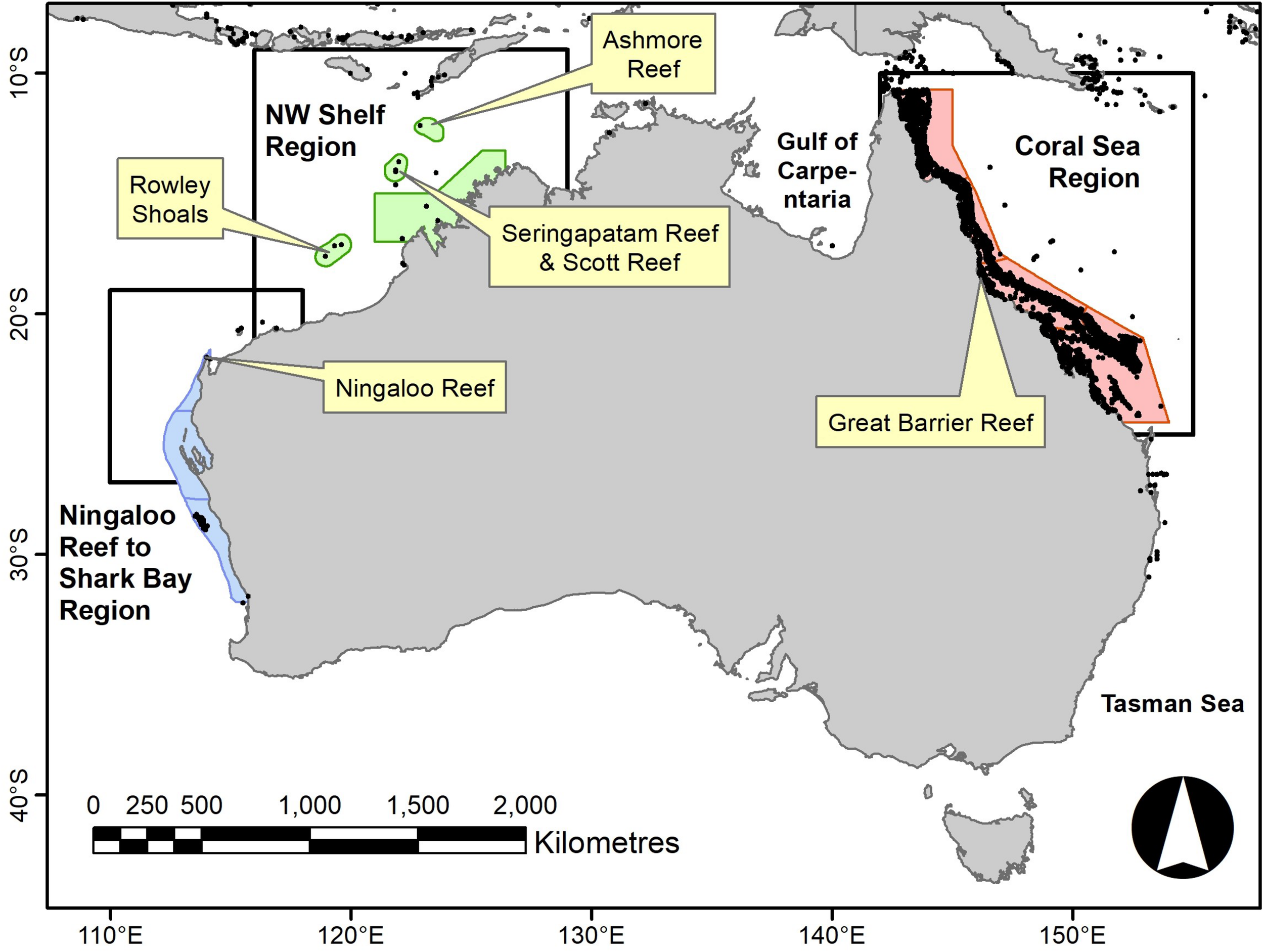
Coral reef regions around Australia included in the thermal stress assessment. Blue grouping denotes reefs on the west coast of WA, green denotes those on the Northwest (NW) Shelf, and red shading encompasses the GBR Marine Park. Reef location data from Tupper et al. (2011).
Seasonal forecasts of ocean temperatures and coral bleaching risk are critical tools for proactive reef management. They provide advance warning of thermal stress events and thus a window for response by reef managers to pre-emptively activate monitoring programs and mitigation options (Spillman, 2011; Spillman et al., 2012; Griesser and Spillman, 2016). Seasonal forecast tools are an integral part of Great Barrier Reef Marine Park Authority’s (GBRMPA) Early Warning System in the Coral Bleaching Response Plan (Maynard et al., 2009; Great Barrier Reef Marine Park Authority, 2013). When increased coral bleaching risk is predicted, an incident response framework is initiated, with a coordinated multi-agency assessment and monitoring program implemented in the case of severe or widespread bleaching (Smith and Spillman, 2019). Seasonal forecast information is used by expert scientific advisory panels as well as to brief reef stakeholders, government, and the public prior to and throughout a mass bleaching event.
The Australian Bureau of Meteorology has been providing operational seasonal SST forecast products out to 6 months for the Great Barrier Reef since 2009 (Spillman et al., 2009; Spillman, 2011). In 2019, this service was upgraded to the new higher resolution (approx 25 km resolution) coupled climate-ocean seasonal prediction system ACCESS-S1 (Australian Community Climate and Earth System Simulator - Seasonal Version 1; Hudson et al., 2017) and expanded to cover all Australian waters. Realtime forecasts of SST anomalies (SSTA), bias corrected SST and new operational thermal stress metrics are provided several times a week online1 (Smith and Spillman, 2019, 2020).
The new ACCESS-S1 operational thermal stress outlooks for Australia are based on two metrics; monthly Hotspots (HS) and Degree Heating Months (DHM) (Spillman et al., 2011, 2012). These metrics both use a reference threshold called the maximum monthly mean (MMM), defined as the warmest monthly climatological value for each pixel over a certain period (Strong et al., 2006). This method is based on the premise that corals are generally acclimatized to a certain local temperature range and when this is exceeded, bleaching can occur. Around tropical Australia, MMM typically occurs in January or February on the GBR, March-April in north western Australia, and December around northern Australia, but can also peak in April due to the bimodal nature of the region (Gilmour et al., 2019; Figure 2A). Monthly Hotspots are defined as positive-only monthly SSTA referenced to the MMM and indicate locations where monthly SST values are warmer than the warmest long-term monthly average (typical warmest summer month).
FIGURE 2
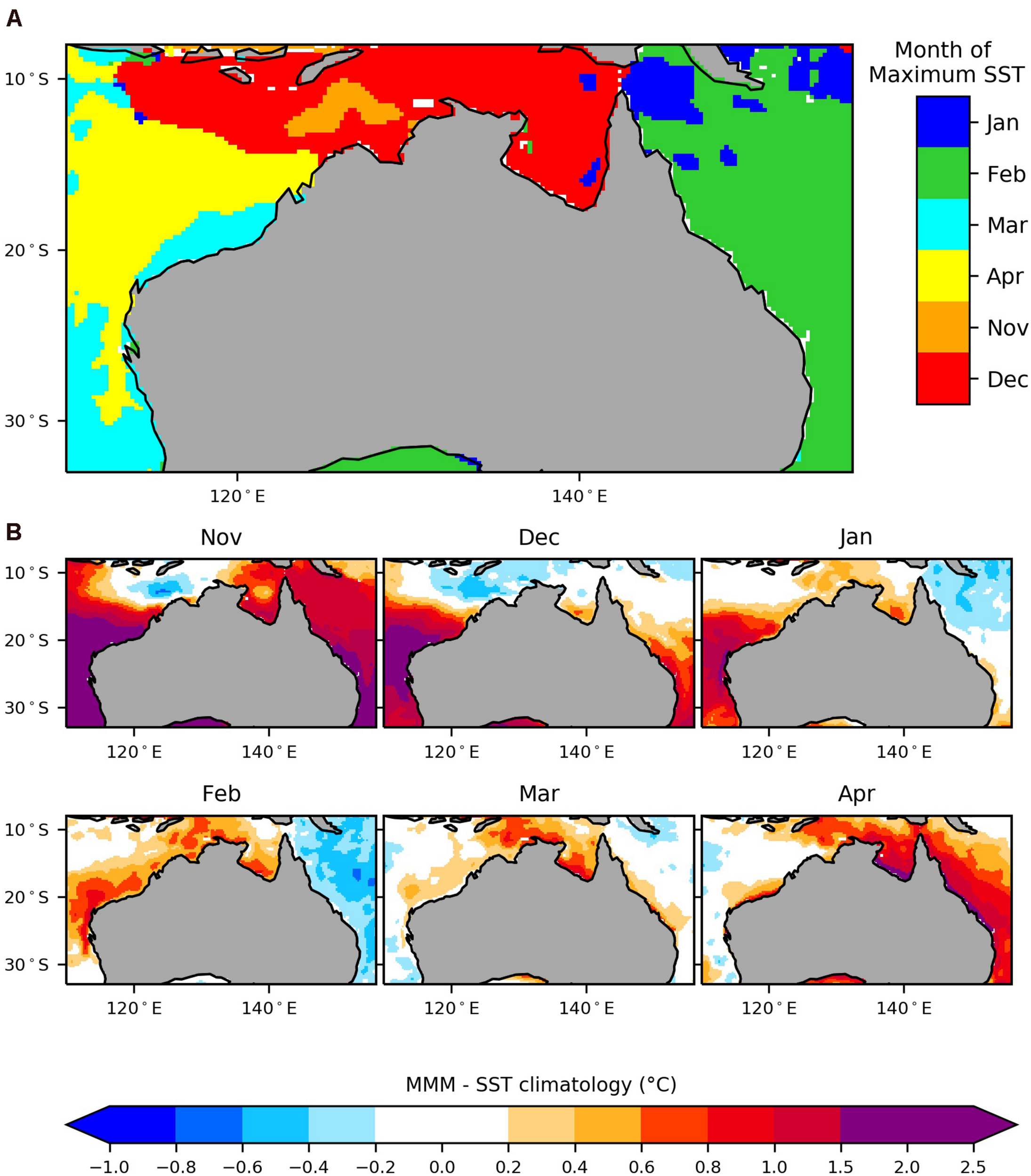
(A) The warmest climatological month for the period 1990–2012 around Australia, based on Reynolds OISSTv2.0 data. (B) Maximum monthly mean (MMM) minus observed OISSTv2.0 monthly SST climatologies for November to April 1990–2012. Negative values indicate where the MMM is cooler than the observed monthly SST climatology, due to detrending of the MMM to November 1988 (see section “Materials and Methods”).
Degree Heating Months are then generated by accumulating monthly HS > 0 oC over a 3 month window (Eakin et al., 2009; Spillman et al., 2012). DHM combine both magnitude and duration of thermal stress, with a DHM value of 1.0 defined as the threshold for a likely bleaching event (Logan and Dunne, 2012). DHM values of 1 and 2 approximately correspond to NOAA Coral Reef Watch Degree Heating Week (DHW) values of 4 and 8 (Spillman et al., 2012), which are the typical thresholds for likely coral bleaching and mortality (Liu et al., 2018). DHWs are calculated by accumulating weekly HS ≥ 1°C values over 12 weeks, as weekly HS < 1 values are not considered sufficient to cause visible stress in corals (Liu et al., 2003, 2005). However, Barton and Casey (2005) found that accumulating monthly HS > 0°C for DHM, rather than HS ≥ 1°C as in DHW calculations, was necessary to capture event signals on monthly timescales. Whilst HS and DHM have been developed as indicators of coral bleaching risk, they have potential applications in fisheries and aquaculture management (Hobday et al., 2016), and can be used as an indicator of marine heatwaves (Benthuysen et al., 2021).
A new operational suite of marine thermal stress products, incorporating HS and DHM metrics and based on ACCESS-S1, are now available for Australian waters. Here, we describe the development, methodology and validation of the new thermal stress products and their application in reef management.
Materials and Methods
ACCESS-S1 details, together with hindcast (retrospective forecast) and realtime configurations, are presented below. Thermal stress forecasts are assessed by comparing a hindcast set for 1990–2012 against satellite SST observations. The NOAA 1/4° Optimal Interpolation SST version 2 (OISSTv2) satellite dataset was used to both validate model forecasts (version 2.1 for 2020 case study) and bias correct forecast SST values (Reynolds et al., 2007; Banzon et al., 2016).
Model Description
ACCESS-S1 is based on the United Kingdom Met Office global seasonal prediction system version five, referred to as GloSea5 (Maclachlan et al., 2015), which includes the latest atmospheric Global Coupled (GC2) model (Williams et al., 2015) coupled with the latest Nucleus for European Modeling of the Ocean (NEMO) community model (Madec and NEMO Team, 2011). Ocean data assimilation uses Forecast Ocean Assimilation Model (FOAM) analyses (Blockley et al., 2014). The ACCESS-S1 ocean grid is tripolar with approximately 25 km × 25 km horizontal resolution in the Australian region (“eddy permitting”, Marsh et al., 2009), with 75 vertical levels with a surface layer thickness of 1 meter. For more details of the ACCESS-S1 set up, see Lim et al. (2016) and Hudson et al. (2017).
Hindcasts were run for the period 1990–2012 for the purpose of forecast verification and bias correction. In the hindcast system, 11 forecasts were run out to 6 months for four start dates (1st, 9th, 17th, and 25th) per month in the hindcast period, using an initial condition perturbation scheme (Hudson et al., 2017). Monthly ocean climatologies were generated by start date and lead time, where lead time is defined as the time between model start date and forecast month (Smith and Spillman, 2019). For example, for a forecast started on 1st January, monthly forecasts at lead times 0, 1, and 2 months are for January, February, and March, respectively. Only forecasts starting on the 1st of the month are considered here. However, to increase the hindcast ensemble size and closer approximate the larger realtime forecast ensemble system, hindcasts starting on the 25th of the prior month were combined with those starting on the 1st of the month to produce a 22-member ensemble (Smith and Spillman, 2019).
The operational realtime forecast system has been running since October 2018 and produces forecasts every day. For monthly forecasts, 11 forecasts out to 6 months are produced daily via perturbation of initial conditions and collated over the previous 9 days to give a 99-member time lagged ensemble (Hudson et al., 2017). An ensemble mean forecast is calculated by averaging all 99 (or 11 in the hindcast set) ensemble members. For a summary of the hindcast and realtime forecast systems, see Table 1.
TABLE 1
| Hindcast | Realtime | |
| Model start dates | 1st, 9th, 17th, and 25th of each month | Daily |
| Period | 1990–2012 | From October 2018 |
| Forecast period | 6 months | 5 or 6 months (5 months for model start dates 1st to 10th of each month, 6 months from the 11th of the month onwards) |
| Ensemble members | 11 perturbed members, combined with 11 perturbed members from 1 previous start date = 22 members | 11 perturbed members, combined with 11 perturbed members from previous 9 daily start dates = 99 members |
| Ocean data assimilated | In situ (Woodruff et al., 2011) and satellite AVHRR and AMSR-E SST (Casey et al., 2010; Maclachlan et al., 2015) sea level altimetry satellite data (Maclachlan et al., 2015), EUMETSAT reanalysis and realtime sea ice concentration data (Maclachlan et al., 2015, http://www.osi-saf.org/) EN3 profile dataset for subsurface temperature and salinity data (Ingleby and Huddleston, 2007) | Realtime equivalent of the hindcast inputs including ARGO, TRITON-TAO array and other moored buoys, expendable bathythermographs (XBTs) and conductivity-temperature-depth (CTD) sensors (Maclachlan et al., 2015) |
| Climatology | 1990–2012 | Choose closest hindcast start date |
| Atmospheric Assimilation (Rawlins et al., 2007) | ERA-Interim (Dee et al., 2009) | Operational Global NWP analysis (Hudson et al., 2017) |
Summary of the ACCESS-S1 realtime and hindcast systems in terms of monthly ocean forecasts.
For further details of the hindcast and realtime forecast systems, see Hudson et al. (2017) and Smith and Spillman (2020).
Monthly forecast SSTA were derived by subtracting their respective lead time dependent model SST climatology for 1990–2012 from SST for all ensemble members (Smith and Spillman, 2019). This process accounts for any model bias with lead time (Stockdale, 1997). Observed monthly SST climatologies for 1990–2012 were derived from the NOAA OISSTv2 dataset and regridded to the model ocean grid. These were then added to model SSTA to provide bias-corrected full field monthly SST forecasts.
Thermal Stress Products
Monthly SSTA form the basis of the thermal stress products presented here, with the important difference that the reference baseline is the MMM, rather than a typical monthly climatology. The MMM dataset utilized here was provided by the United States. National Oceanic and Atmospheric Administration (NOAA) Coral Reef Watch (CRW), and derived from Optimum Interpolation SST version 2 (OISSTv2) data (Liu et al., 2018). The original MMM used in relating temperature stress and bleaching responses was based on the period 1985–1993 (excluding 1991 and 1992 due to Mt Pinatubo eruptions) (Liu et al., 2003). The MMM includes data for the period 1985–2006, omitting 1991 and 1992, and detrended to November 1988 (middle date of the original MMM) to maintain consistency with earlier MMM versions (Heron et al., 2014b; Liu et al., 2014). Note that the OISSTv2-based MMM used in this study is a different product to the Pathfinder-based MMM (Casey et al., 2010; Heron et al., 2014a) currently used in the operational ACCESS-S1 DHM forecasts (Smith and Spillman, 2020). Future upgrades of the operational system will also include a migration to the OISSTv2 based MMM.
Detrending of the MMM to November 1988, however, means that it is possible for monthly observed climatologies for 1990–2012 to be warmer than the MMM in summer in some regions. This can be seen in Figure 2B, where January and February observed SST climatologies are actually 0.4oC warmer than the MMM in the Coral Sea, and similarly in March and April on the west coast.
Hotspots were calculated for all ensemble members and ensemble mean by finding the difference between the full field bias-corrected monthly SST forecast values and MMM with all negative values set to zero:
where, lt is lead time from 0 to 5 months and t is model start date. HS values were generated for all ensemble members and the ensemble mean. Monthly HS values were also calculated for observations using monthly OISSTv2.0 SST and MMM.
Degree Heating Months were calculated by summing HS values over consecutive 3 months period (Spillman et al., 2012) for each location:
where, lt is lead time 0 to 3 months and t is model start date. For example, at lead time 0 months DHM is the accumulation of HS at lead times 0, 1, and 2 months (Spillman et al., 2012; Smith and Spillman, 2020). DHM values were calculated for all ensemble members and the ensemble mean. However, it is important to note that only forecasts for full calendar months are used in HS and DHM calculations. Operationally, realtime DHM forecasts produced after the 1st of the month are an accumulation of HS forecasts for the next three full months, i.e., a DHM forecast produced on February 02, accumulates the monthly HS forecasts for March, April, and May. Observed DHM were calculated by summing three consecutive monthly HS in the period (Smith and Spillman, 2020).
Reference forecasts were also calculated to provide a skill benchmark (see Spillman and Alves, 2009). The two most commonly used reference forecasts, climatology and persistence are both relatively easy to beat since a positive DHM can be deemed as an extreme or rare event in certain regions and therefore difficult to predict by persisting a previous month that is most likely warmer or cooler seasonally, or climatology which averages out the extremes. A more difficult reference forecast to beat, and the one chosen for this assessment, is a combination of persistence and climatology. They were created by persisting the observed SST anomaly from the month prior to the start date (i.e., December for a start date of January 01) out to 6 months into the future. The relevant observed monthly climatologies were added before the MMM was removed to create HS, which were then summed over a 3 months window to give quasi DHM persistence forecasts.
Validation of Thermal Stress
To evaluate forecast skill, hindcast DHM values were compared to those derived from the NOAA 1/4° OISST dataset for 1990–2012 using a range of metrics. Pearson correlation coefficients of SSTA for the hindcast period at lead times 0 to 5 months during November to April in the Australian region is presented as a baseline assessment of skill. Root mean square error (RMSE) values were also calculated. All thermal stress metrics are derived from SSTA and therefore can only be skilful if there is good skill in the underlying parameters on which they are based. It is also important to note that the skill of the hindcast set is assumed to approximate that of the operational realtime system, despite the different ensemble generation schemes, as there is not sufficient realtime forecasts to undertake a skill assessment.
Hotspots are more likely to occur in summer months as the MMM baseline is based on the warmest climatological month. The frequency distribution is skewed as HS values of zero are much more common over the course of a year than positive HS values. As HS are most likely to occur during the warmer summer months, thermal stress forecasts were assessed for November to April (Figure 3). To assess whether the model correctly predicted an observed DHM > 0 value, if more than 50% of ensemble forecasts indicated DHM > 0 then this was termed a “hit.” Conversely if less than 50% of members correctly predicted DHM > 0 then this was termed a “miss.” These “hit” and “miss” counts can be combined to calculate the hit rate as follows:
FIGURE 3
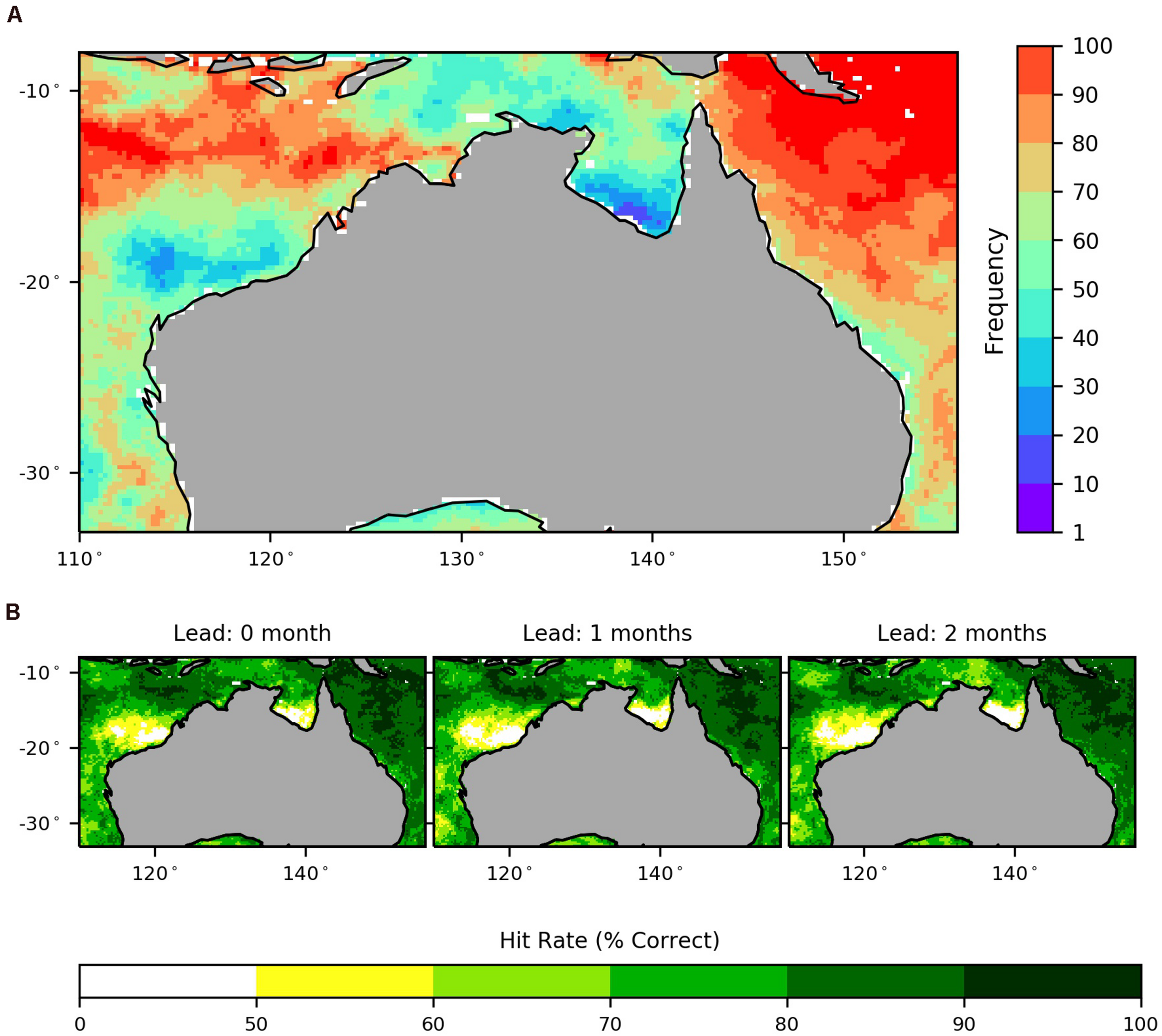
(A) Observed frequency of DHM > 0 events for November to April 1990–2012, together with (B) model hit rates for DHM > 0 for the same period for lead times 0–2 months (total number of months = 138). Note that an event is considered to have been forecast if more than 50% of ensembles have indicated DHM > 0 at a location.
where, x,y is the grid point location, lt is lead time, and t is model start dates for all November to February forecasts in the hindcast period (note that a DHM forecast issued on February 01 includes HS forecasts from February 01 for February, March, and April). DHM forecasts starting March 01 (i.e., March to May) and April 01 (i.e., April to June) were not included as they fell outside the November to April window. Hit rates remove any skill bias by not incorporating correct negatives (i.e., model correctly predicting no DHM > 0) into the calculation.
The term reliability is a attribute of probabilistic skill that refers to the ability of the model to match forecast probabilities with the observed frequencies (Wilks, 1995), and is assessed by using a reliability diagram which gives an indication of how well forecast probabilities and observed frequencies adhere to a 1:1 relationship. Reliability diagrams also provide information on model resolution, which is the probabilistic skill of model forecasts over climatology. Resolution is indicated on the reliability diagram by a shaded region, with points falling within contributing positively to the Brier Skill Score (BSS), equation 5.
The Brier score (BS) gives a measure of overall probabilistic model skill against observations (Brier, 1950):
where, N is the number of samples, pi is the forecast probability, and oi is the observed occurrence (either 0 or 1). The range of BS values is 0 to 1, with 0 being a perfect score. For rare events, it becomes easier to get a good BS without having any real skill. The BSS gives an indication of the skill of the probabilistic forecast compared to the reference forecast (Wilks, 2006);
where, BSref is the Brier score of the reference forecast. The reference forecast used here is persistence (see section “Thermal Stress Products”). A value of 0 or less suggests no skill compared to using our chosen reference forecast, as defined in the previous section, with 1 a perfect score.
All probabilistic skill assessments outlined above defined events using the thresholds DHM > 0, DHM > 1, and DHM > 2. Hit rates, reliability diagrams, and BSS values were calculated for all grid cells across tropical Australia (north of 28 °S) for November to April 1990–2012 at lead times 0 to 2 months.
To assess the model’s ability to predict the spatial extent of a DHM event, the number of grid cells within certain regions where the model predicted DHM > 1 in the ensemble mean (with ensemble range included i.e., minimum/maximum) was compared to that observed for each start month in 1990–2012 at lead 0 months (Figure 4). The percentage region calculation is as follows:
FIGURE 4
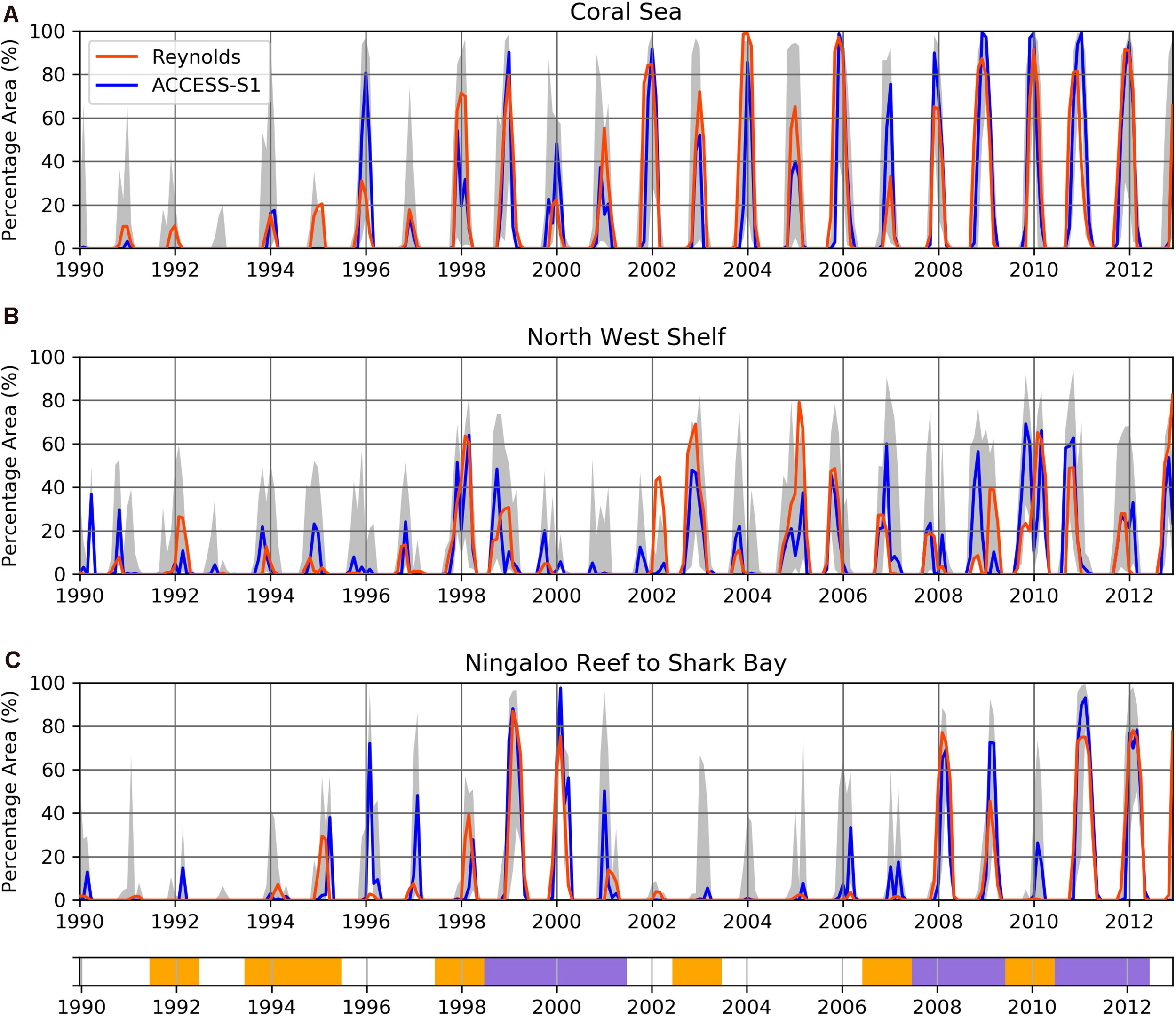
Percentage of each region where DHM > 1 were observed and predicted for the (A) Coral Sea, (B) NW Shelf, and (C) Ningaloo to Shark Bay for 1990–2012 at lead time 0 month. Yellow shading indicates timing of El Niño events and purple shading La Niña events, as per Bureau of Meteorology definitions (http://www.bom.gov.au/climate/enso/enlist/). Gray shading shows the ensemble range. See Figure 1 for locations of regions.
where, t is model start date. The total number of grid cells in the percentage equation refers to the number of ocean grid cells within the box regions shown in Figure 1. Grid cells within the regions were all very similar in size (approximately 0.25 degrees).
Additionally, two case studies highlighting the most significant coral bleaching events in the Australian region during the hindcast period are presented: in 1998 on the Great Barrier Reef and the North West (NW) Shelf (i.e., Scott Reef; Case Study 1), and in 2011 on the west coast of Australia (i.e., Ningaloo Reef, Shark Bay, Abrolhos Island; Case Study 2). Additionally, a third case study looking at the 2020 Great Barrier Reef coral bleaching event, using realtime operational forecasts, is also presented (Case Study 3).
Results
Correlations between model and observed SSTA are shown in Figure 5A for November-April 1990–2012 for leads 0–5 months. Correlations are highest at lead 0 months and decline with lead time. At lead 0 model skill is highest on the central and southern coast of Western Australia, the east coast and Coral Sea, whereas skill is lowest on the NW Shelf and in the Gulf of Carpentaria (Figure 5). Skill rapidly decays for the two latter regions with lead and is less than 0.3 inshore by lead 3 months. Conversely, skill remains above 0.5 out to lead 5 months for most of the Coral Sea and the southern WA coast. When the 6 months assessed are considered individually, skill tends to be higher for most regions around Australia for November and April, with lowest skill for February, especially at longer lead times (not shown). RMSE values are also shown in Figure 5B, with lowest values (more skilful) across northern Australia and the Coral Sea, and higher values (less skilful) on the southern WA coast, where variability is higher. RMSE values are lowest for lead 0 months, with higher and similar values across leads 1–5 months.
FIGURE 5
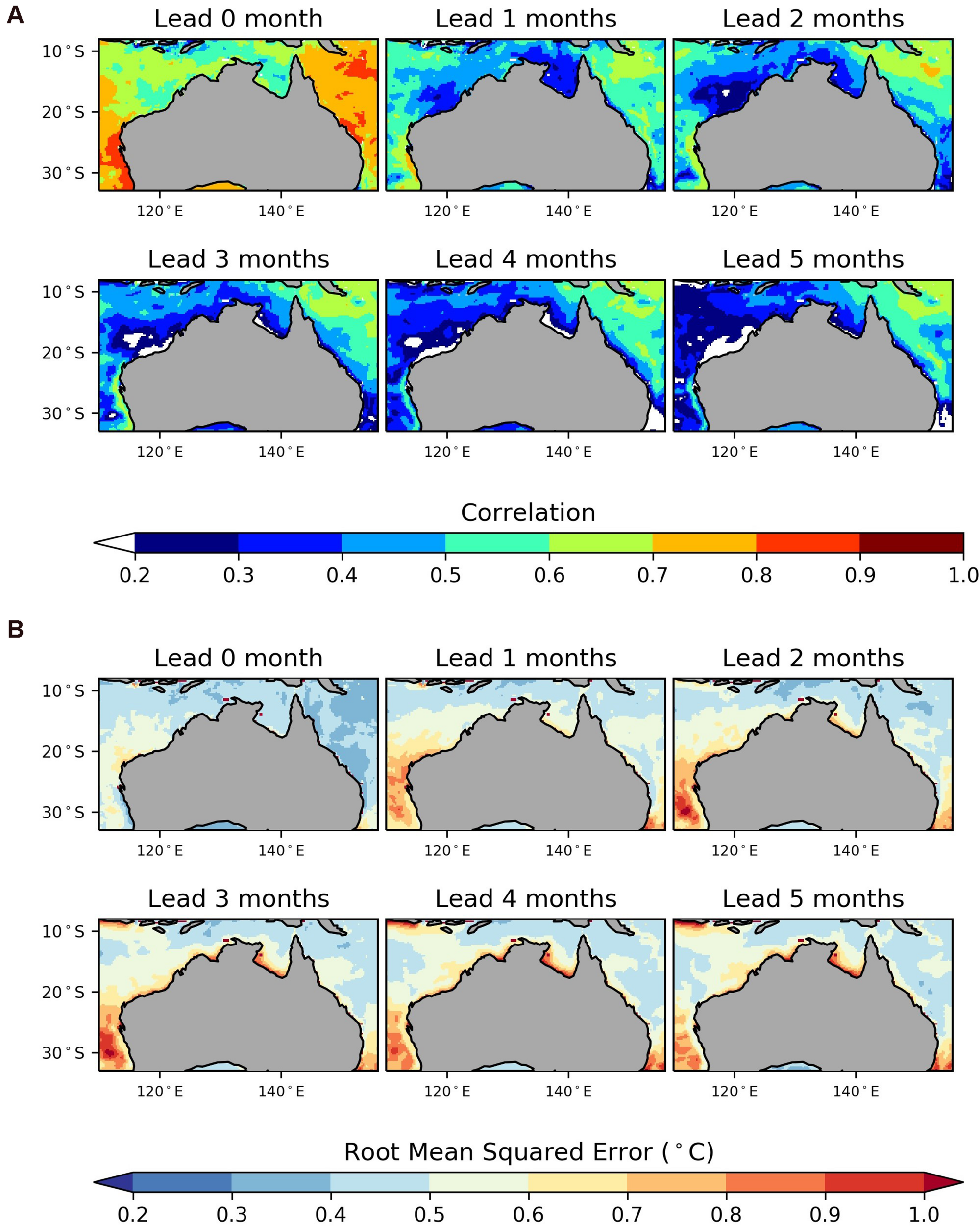
(A) Correlations and (B) root mean square errors (RMSE) for comparisons of forecast and observed monthly SSTA values for November to April 1990–2012 at lead times 0–5 months. Correlations > 0.2 are statistically significant and shaded (N = 23 years × 6 months, p = 0.05).
Model hit rates for DHM > 0 in November to April 1990–2012 for lead times 0–2 months are shown in Figure 3. A score of 100% indicates that the model correctly predicted all occurrences of DHM > 0 observed. At lead time 0, hit rates for DHM > 0 exceed 60% for most of the domain with hit rates above 80% in the Coral Sea and small regions north of the Kimberley including Scott and Ashmore Reefs (Figure 3B). The exceptions are north west WA and the Gulf of Carpentaria, where hit rates are low for all leads. This is most likely due to a comparatively low occurrence of DHM > 0 in both these regions (Figure 3A), as well as low skill at most lead times (Figure 5). Hit rates remain above 60% in the Coral Sea, northern GBR and the west and southern WA coast out to 2 months lead.
Reliability diagrams with Brier Skill Scores are shown for DHM > 0, DHM > 1 and DHM > 2 for November-April 1990–2012 in Figure 6. Possible BSS skill values range from 0 (poor skill c.f. reference forecast) to 1 (perfect skill). All reliability curves shown here largely fall within the shaded region, which indicates positive contributions to the BSS. As the DHM threshold increases from 0 to 2, the reliability curves flatten out though remain in the shaded region, resulting in BSS values of 0.45 to 0.55. Perfectly reliable forecasts would lie along the 1:1 line, however, here values drift below this line as the DHM threshold increases. This indicates that the model is under-dispersive and is over-forecasting i.e., model probabilities are consistently higher than observed frequencies and as such, the model is overconfident. The BSS is stable with lead time for all thresholds, showing that the model DHM probabilistic skill beats that of the reference DHM persistence forecasts (see section “Materials and Methods” for calculation).
FIGURE 6
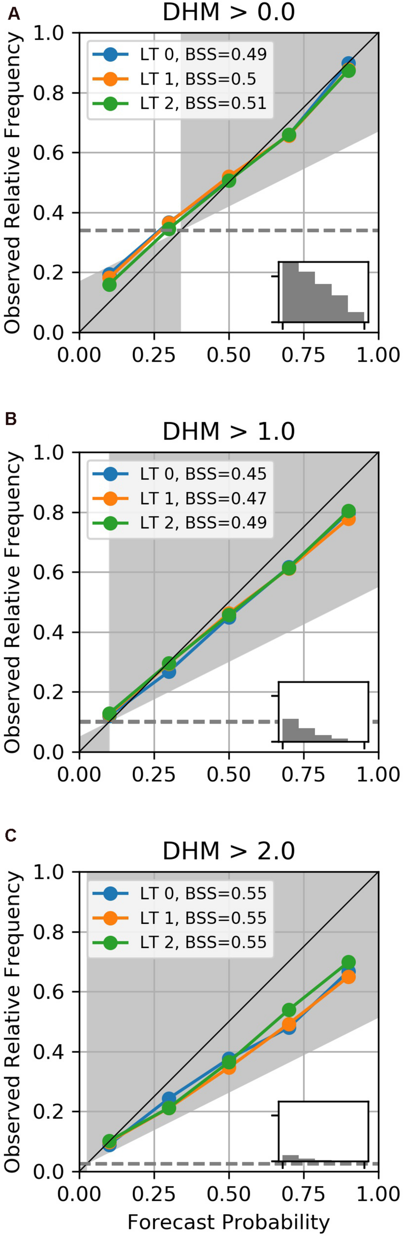
Reliability diagram for (A) DHM > 0, (B) DHM > 1, and (C) DHM > 2 for November to April 1990–2012 for lead times 0–2 months, using a 22 member ensemble. Domain is the whole of northern Australia as shown Figure 1. Brier Skill Scores (BSS) and bar charts showing observed occurrences for each 0.2 frequency bin are also included. Reference forecast used is DHM quasi-persistence for the same period (see section “Materials and Methods” for calculation).
Figure 4 shows the proportion of grid cells within each region where DHM > 1 is observed and predicted for the Coral Sea, NW Shelf and Ningaloo Reef to Shark Bay for 1990–2012 at lead time 0 months (see Figure 1 for regional outlines). In bleaching years 2002 and 2006 in the Coral Sea, the proportion of grid cells where DHM > 1 was predicted was close to that observed, i.e., 85 and 95%, respectively (Figure 4A). However, in 1998 the extent of DHM > 1 was underpredicted by the model by more than 50% as the start date moved into January. Later in the period, the extent of the Coral Sea where DHM > 1 was instead overpredicted by 5 to 20 % for non-bleaching event years 2009 to 2011. The timing of peak extent in the Coral Sea was predicted later than observed in several years, particularly 2002 and 2004. On the west coast, the predicted timing of peak extent was more consistent with observed on both the NW Shelf and at Ningaloo/Shark Bay (Figures 4B,C). The bimodal peak in temperatures on the NW Shelf can be observed in summers of 1998/1999, 2009/2010, and 2010/2011. ACCESS-S1 forecasted the second peak in spatial extent later in the summer in the region but consistently struggled to forecast the first peak in early summer in these years. For summers in 2007 to 2011 the model overpredicted the area on the NW Shelf where DHM > 1 (Figure 4B), as was seen for the Coral Sea. Six of the 23 summers in the Ningaloo/Shark Bay region recorded peaks of more than 60% of the area with values of DHM > 1 (Figure 4C). The model captured the timing and magnitude of the four largest peaks in 1999, 2000, 2008, 2011 and 2012, all of which occurred during a La Niña. The model did, however, overpredict the spatial extent in 1996, 1997, and 2001, all ENSO neutral summers.
Two hindcast case studies are presented for bleaching events on the GBR and Scott Reef in 1998 (Case Study 1; Figure 7) and Ningaloo Reef in 2011 (Case Study 2; Figure 8). Warming was observed on both the west and east coasts of Australia in February-March-April (FMA) 1998 during the 1997/1998 El Niño (Figure 7, bottom row). On the east coast, elevated DHM values were forecast in the southern GBR for all lead times shown, although the peak magnitudes were not captured by the ensemble mean even at lead time 0. In the probabilistic forecasts, however, 50% or more of ensemble members indicated DHM > 1 in the southern GBR for all lead times shown (Figure 7, right column). The thermal stress observed to the north of the GBR was not predicted at any lead time.
FIGURE 7
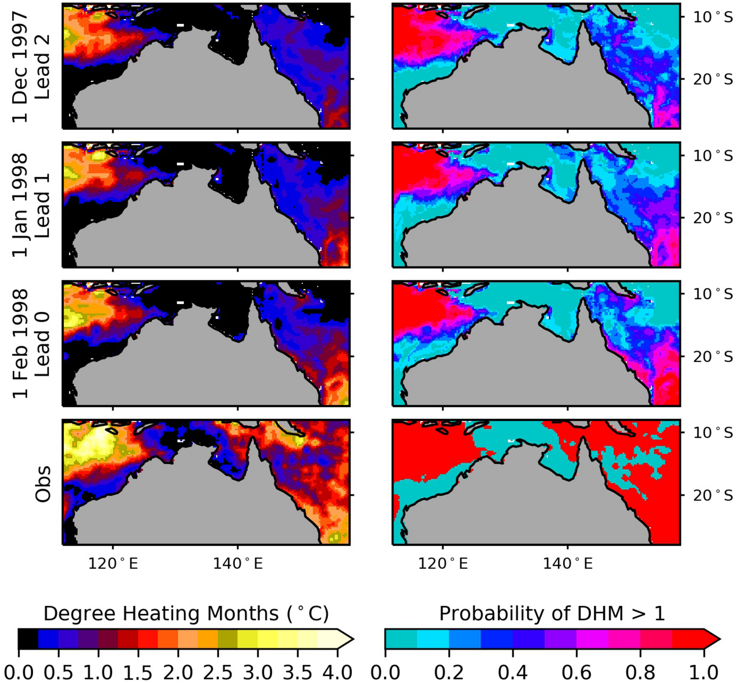
Case Study 1: Hindcast DHM forecasts for Northern Australia for February to April 1998 for model start dates 1 December 1997, 1 January 1998, and 1 February 1998. Left column is ensemble mean DHM, right column is probability of DHM > 1, using 22 ensemble members. Observed DHM values for February to April 1998 are shown in the bottom row.
FIGURE 8
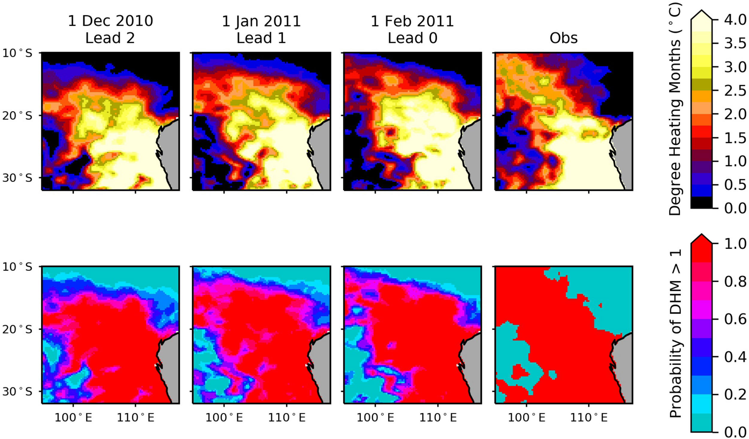
Case Study 2: Hindcast DHM forecasts for Ningaloo for February to April 2011 for model start dates 1 December 2010, 1 January 2011, and 1 February 2011. Top row is ensemble mean DHM, bottom row is probability of DHM > 1, using 22 ensemble members. Observed DHM values for February to April 2011 are shown in the far-right column.
In the west, the model better captured observed DHM values in both Case Study 1 (Figure 7) and Case Study 2 (Figure 8). DHM values observed on the NW Shelf in February to April 1998 were generally well forecast in terms of magnitude, location and timing at all lead times (Figure 7, left column). Conditions at Rowley Shoals and Scott Reef were well captured, however, ensemble mean DHM values did not quite reach observed magnitudes at Ashmore Reef. Probabilistic forecasts of DHM > 1 (Figure 7, right column) indicated at least 80% of ensemble members exceeded 1 DHM at Scott Reef for all start dates. In Case Study 2 during the 2011 marine heat event from Ningaloo to Abrolhos Islands, a maximum of 3.6 DHM was observed in the Ningaloo region, with even higher DHM values up to 10 observed near Shark Bay and Abrolhos Islands. ACCESS-S1 did an excellent job in capturing both the magnitude and spatial extent of DHM values at all lead times (Figure 8; Case Study 2).
Operational realtime forecasts are presented in Case Study 3 for the 2020 GBR coral bleaching event in Figure 9. When compared to observations, the predicted peak of the 2020 event matches well in terms of extent in the central and northern GBR. Probabilistic forecasts indicated a 60% or higher chance of DHM > 1 values occurring in the central and northern GBR at all lead times. The forecast probability of DHM > 1 occurring in January-March 2020 increased to above 80% for December 01 and January 01 start dates, with lead time 0 forecasting ensemble mean DHM of up to 2 in the GBR Marine Park. However, the magnitude of observed DHM values were underpredicted by approximately 50% (in the order of 1.75 DHM).
FIGURE 9
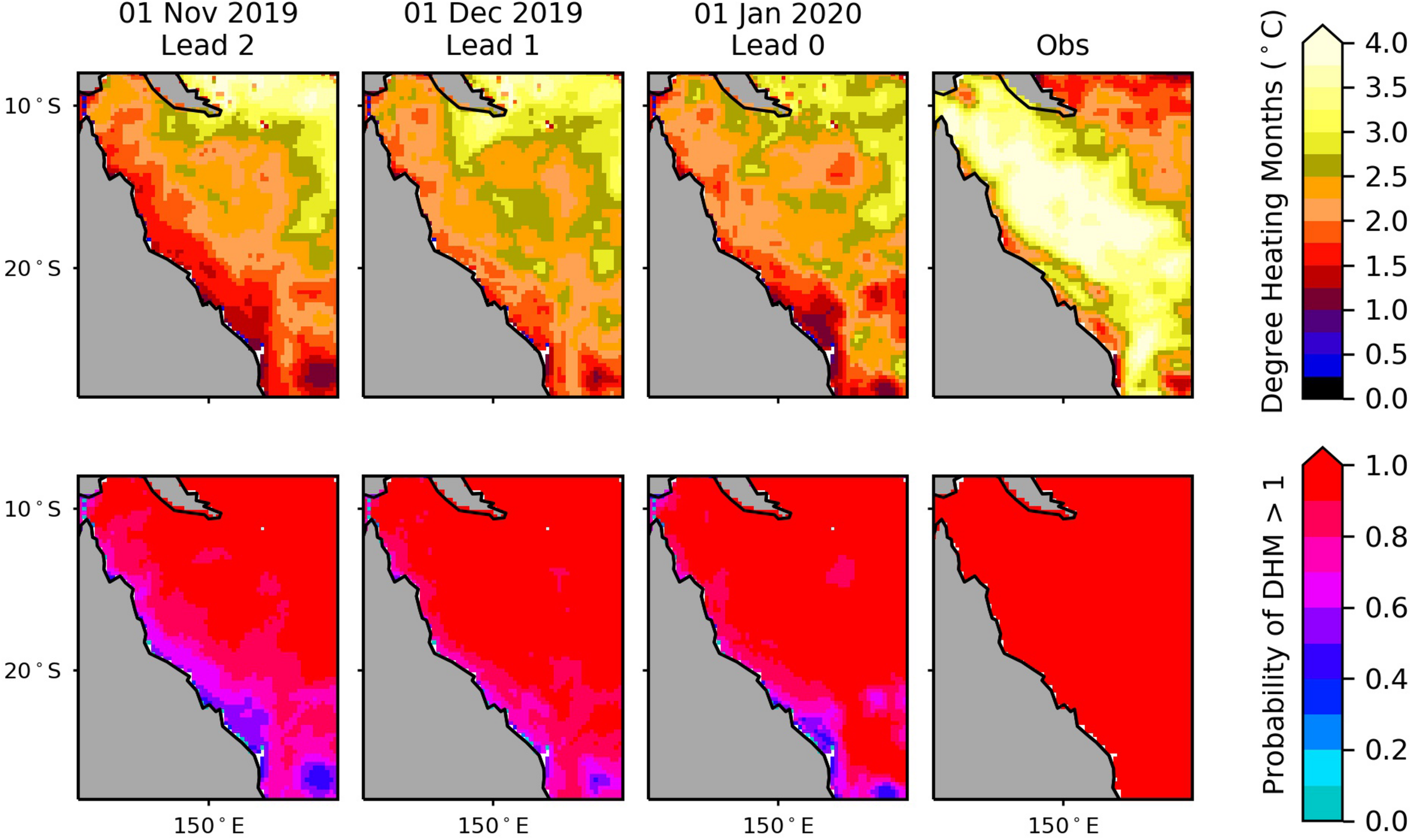
Case Study 3: Realtime DHM forecasts for the GBR for January to March 2020 for model start dates 1 November 2019, 1 December 2019, and 1 January 2020. Top row is ensemble mean DHM, bottom row is probability of DHM > 1, using 99 ensemble members. Observed DHM values for January to March 2020 are shown in the far-right column.
Discussion
Coral reefs around Australia have experienced heat induced mass coral bleaching in recent years, due to the large-scale climate drivers such as ENSO, regional mesoscale weather patterns and warming ocean temperatures due to climate change. Spatial extent, duration, and timing of marine heat events in reef regions vary around Australia and are influenced by oceanography, local weather and teleconnections with larger scale climate drivers. Forecasting thermal stress events on seasonal timescales is an important tool for reef managers to effectively implement monitoring and management initiatives in these vulnerable regions. The Australian Bureau of Meteorology has been providing operational thermal stress outlooks for coral bleaching risk, based on the new higher resolution ACCESS-S1, since 2018.
Model thermal stress forecasts were most skilful in the Coral Sea, northern GBR and the central and southern coast of WA for November to April over the hindcast period 1990–2012. Conversely lowest DHM skill was seen for the NW Shelf and Gulf of Carpentaria. In this study, during the hindcast period thermal stress predictability was highest when regions have strong ENSO teleconnections with strong heat advection (e.g., 2011 Ningaloo Niño), moderate with ENSO teleconnections with primarily air-sea flux mechanisms (e.g., GBR during 1998 El Niño), and poorest with neither strong ENSO teleconnections nor heat advection (e.g., GBR in ENSO neutral years). In terms of probabilistic skill, tropical northern Australia showed improved skill over the reference DHM persistence forecast for DHM > 0, 1 and 2 events. BSS values were in the range deemed good to very good for all lead times and thresholds. Forecasts also exhibited similar probabilities to the observational occurrences providing evidence of forecast reliability, although the forecast became more overconfident at higher thresholds, a similar finding to that for higher SSTA thresholds in Smith and Spillman (2019). These DHM thresholds are useful for reef managers as DHM values of 1 and 2 approximately correspond to NOAA Coral Reef Watch DHW values of 4 and 8 (Spillman et al., 2012) which are the typical thresholds for likely coral bleaching and mortality (Liu et al., 2018).
The model captured the GBR marine heat events of 1998 and 2020, though tended to underestimate the peak magnitude and extent of both events. Smith and Spillman (2019) showed that SST skill was highest in the GBR when forecasting larger warm anomalies in the GBR associated with longer lived climate drivers (e.g., ENSO events), rather than regional weather. Historically, mass bleaching events on the GBR have typically associated with El Niño events, however, 2020 was an ENSO neutral year, as was 2017 which also saw mass coral bleaching (Hughes and Kerry, 2017). Despite the lack of large climate drivers, the model still captured warming in the GBR in 2020 though not at observed magnitudes. ACCESS-S1 forecasts were used operationally in 2020 by the GBRMPA to coordinate and inform their responses to the bleaching event, including ministerial and stakeholder briefings and multi-agency coordination of surveys.
The thermal stress associated with the Ningaloo Niño of 2011 (Feng et al., 2013) was well captured by the model off the west coast of WA (Figure 8). DHMs reached a maximum of 3.6 DHM in the Ningaloo region, which is of a similar magnitude as the GBR event in 2020. Further south much higher DHMs of up to 10 were observed, which was also identified as one of few observed category 5 marine heatwave (MHW) events (Holbrook et al., 2020). This event led to mass coral bleaching, fish kills, and sea grass die off (Caputi et al., 2014). Bleaching was also reported in 2012 at Ningaloo, however, was far less severe than 2011 due to amount of coral mortality that had already occurred the previous year (Babcock et al., 2017). The teleconnection between thermal stress events at Ningaloo and La Niña events in the Pacific is evident in Figure 4C. Six of the largest thermal stress events occurred during moderate to strong La Niña years (1998/1999, 1999/2000, 2007/2008, 2008/2009, 2010/2011, and 2011/2012). During a La Niña, warm water builds up in the western Pacific, flows through the Indonesian throughflow and down the WA coast. This results in a warmer, stronger Leeuwin Current, modulated by associated wind anomalies inducing coastal downwelling (Kataoka et al., 2014), and increasing the likelihood of a Ningaloo Niño (Feng et al., 2008). The La Niña of 2020/2021 resulted in high SSTs down the coast of WA during the 2020/2021 summer, which were predicted by operational ACCESS-S1 forecasts.
In contrast to Ningaloo and the southern WA coast, model forecast skill for the NW Shelf was notably low by all measures used here. Thermal stress at Scott Reef summer of 2001/2002, 2002/2003, and 2004/2005 was not well forecast in terms of the ensemble mean. Zhang et al. (2017) assessed marine heat wave (MHW) events at Scott Reef in terms of intensity and duration. The years 2001 to 2005 were characterized by a series of shorter duration (17 days) high intensity events over 2 to 3 months, whereas most other MHW events occur closer to or over 1 month durations during the December to April period. Shorter duration events are more challenging for ACCESS-S1 to forecast. Although they contribute to the monthly observation values, they are not well represented in the forecast which performs better for events that persist for 1 month or longer. Additionally, the peak SST month of the year in the region, used to derive the MMM, changes several times over the region (Figure 2A), and the circulation in the region is relatively complex.
Ensemble mean forecasts are often used as a deterministic forecast because they are relatively simple to interpret by a wide range of users, though they contain no measures of uncertainty or the likelihood of alternative outcomes and so are less useful (Tommasi et al., 2017). The ensemble mean forecast does not always predict observed events, as can be seen in this study. However, observed DHM extent were almost always captured by the model ensemble spread for the three selected locations in Figure 4, including less skilful forecasts for the NW Shelf. The full forecast ensemble was used to produce HS and DHM metrics in order to assess the probability of exceedance for particular thermal stress thresholds. The level of ensemble spread, as well as the number of forecast ensemble members predicting a particular event, give insight into model forecast confidence. Probabilistic skill measures indicated the model had good reliability and skill over quasi-persistence, and therefore useful skill.
Typical coral bleaching thresholds, such as MMM, used to construct accumulated thermal stress metrics may not be appropriate in future under a warming climate. In fact, the MMM may already be no longer the best choice for regions where significant warming has occurred. In areas such as the Coral Sea and the west coast of WA, which show the highest positive SST trends (Hobday and Pecl, 2014), it is possible for negative SSTA to positively contribute to DHM values (Figure 2). This essentially means that the monthly observed climatologies for the more recent period of 1990–2012 are already significantly warmer than the MMM, due to the detrending of the MMM to November 1988 It is also possible that the critical thresholds are changing due to coral adaptation or species composition responses to warming oceans (Császár et al., 2010; Kubicek et al., 2019). This baseline was adopted to construct the ACCESS-S DHM product as reef managers were already familiar with the reference baseline and the products could be more easily compared with those produced by NOAA Coral Reef Watch2. However, the predictive capacity of the current DHM definition to indicate coral bleaching severity is likely to vary around Australia and so future iterations may utilize a different baseline. Preliminary research on seasonal prediction of marine heatwaves, utilizing the Hobday et al. (2016) definition, offers wider application and may be a more useful predictor of coral bleaching risk, particularly in areas of high SST variability such as the WA coast (Benthuysen et al., 2021).
The likelihood of a marine heat event as indicated by high DHM values, together with forecast skill, can be utilized by reef managers in risk-based management responses. An early warning system for coral bleaching risk is useful for reef managers as it allows a window of time to implement strategies and allocate potential resources for adequate monitoring and reduce additional stressors on affected reef regions. These products have become integral parts of the GBRMPA Early Warning System for coral bleaching. The product suite will be upgraded to the next version of ACCESS-S (version 2) in 2021, which will have the added benefit of a longer hindcast period (that will include the 2016 and 2017 GBR bleaching events) and model system improvements that are expected to improve model skill. Skilful forecast of thermal stress for coral bleaching risk will increase in their value and importance for proactive marine management in a warming climate.
Statements
Data availability statement
The raw data supporting the conclusions of this article will be made available by the authors on request, without undue reservation.
Author contributions
CS wrote the body of the text and provided scientific direction for the manuscript. GS performed the data analysis, produced the figures, and provided feedback on text. Both authors contributed to formatting and referencing.
Acknowledgments
We appreciate the assistance of Griffith Young, Morwenna Griffiths, and Guo Liu for the preparation of the ACCESS-S1 hindcast set, and Xiaobing Zhou and Matthew Wheeler (Bureau of Meteorology, Australia) for review of an earlier draft.
Conflict of interest
The authors declare that the research was conducted in the absence of any commercial or financial relationships that could be construed as a potential conflict of interest.
References
1
Arias-Ortiz A. Serrano O. Masqué P. Lavery P. S. Mueller U. Kendrick G. A. et al (2018). A marine heatwave drives massive losses from the world’s largest seagrass carbon stocks.Nat. Clim. Change8338–344. 10.1038/s41558-018-0096-y
2
Babcock R. C. Bustamante R. H. Fulton E. A. Fulton D. J. Haywood M. D. E. Hobday A. J. et al (2019). Severe continental-scale impacts of climate change are happening now: extreme climate events impact marine habitat forming communities along 45% of Australia’s coast.Front. Mar. Sci.6:411. 10.3389/fmars.2019.00411
3
Babcock R. C. Thomson D. Haywood M. Vanderklift M. Pillans R. Rochester W. et al (2017). Multi-Year Coral Bleaching Episode in NW Australia and Associated Declines in Coral Cover, Pilbara Marine Conservation Partnership – Final Report.Brisbane, OLD: CSIRO Oceans and Atmosphere, 472–491.
4
Baker A. C. Glynn P. W. Riegl B. (2008). Climate change and coral reef bleaching: an ecological assessment of long-term impacts, recovery trends and future outlook.Estuar. Coast. Shelf Sci.80435–471. 10.1016/j.ecss.2008.09.003
5
Banzon V. Smith T. M. Mike Chin T. Liu C. Hankins W. (2016). A long-term record of blended satellite and in situ sea-surface temperature for climate monitoring, modeling and environmental studies.Earth Syst. Sci. Data8165–176. 10.5194/essd-8-165-2016
6
Barton A. D. Casey K. S. (2005). Climatological context for large-scale coral bleaching.Coral Reefs24536–554. 10.1007/s00338-005-0017-1
7
Benthuysen J. A. Steinberg C. Spillman C. M. Smith G. A. (2021). Oceanographic Drivers of Bleaching in the GBR: From Observations to Prediction. Observations and Predictions of Marine Heatwaves: Report to the National Environmental Science Program.Cairns, OLD: Reef and Rainforest Research Centre Limited, 46.
8
Blockley E. W. Martin M. J. McLaren A. J. Ryan A. G. Waters J. Lea D. J. et al (2014). Recent development of the Met Office operational ocean forecasting system: an overview and assessment of the new Global FOAM forecasts.Geosci. Mod. Dev.72613–2638. 10.5194/gmd-7-2613-2014
9
Brier G. W. (1950). Verification of forecasts expersses in terms of probaility.Month. Weather Rev.781–3. 10.1175/1520-0493(1950)078<0001:vofeit>2.0.co;2
10
Brown B. E. (1997). Coral bleaching: causes and consequences.Coral Reefs16S129–S138. 10.1007/978-3-540-69775-6_1
11
Bruno J. F. Selig E. R. Casey K. S. Page C. A. Willis B. L. Harvell C. D. et al (2007). Thermal stress and coral cover as drivers of coral disease outbreaks.PLoS Biol.5:1220–1227.
12
Caputi N. Jackson G. Peace A. (2014). The Marine Heat Wave off Western Australia during the Summer of 2010/11 – 2 Years On, Fisheries Research Report [Western Australia].Perth, WA: Department of Fisheries, Western Australia.
13
Casey K. S. Brandon T. B. Cornillon P. Evans R. (2010). The past, present, and future of the AVHRR pathfinder SST program.Oceanogr. Space Revis.10273–287. 10.1007/978-90-481-8681-5_16
14
Coles S. L. Kandel F. L. M. Reath P. A. Longenecker K. Eldredge L. G. Eldredge L. G. (2006). Rapid assessment of nonindigenous marine species on coral reefs in the main Hawaiian Islands.Pac. Sci.60483–507. 10.1353/psc.2006.0026
15
Császár N. B. M. Ralph P. J. Frankham R. Berkelmans R. van Oppen M. J. H. (2010). Estimating the potential for adaptation of corals to climate warming.PLoS One5:e9751. 10.1371/journal.pone.0009751
16
Dee D. P. Berrisford P. Poli P. Fuentes M. (2009). ERA-Interim for climate monitoring.ECMWF Newsletter1195–6.
17
Done T. Turak E. Wakeford M. De’ath G. Kininmonth S. Wooldridge S. et al (2002). Testing bleaching resistance hypotheses for the 2002 Great Barrier Reef bleaching event.Test2:95.
18
Eakin C. M. Lough J. M. Heron S. F. (2009). “Climate variability and change: monitoring data and evidence for increased coral bleaching stress,” in Coral Bleaching: Patterns, Processes, Causes and Consequences, edsvan OppenM. J. H.LoughJ. M. (Berlin: Springer), 41–67. 10.1007/978-3-540-69775-6_4
19
Feng M. Biastoch A. Böning C. Caputi N. Meyers G. (2008). Seasonal and interannual variations of upper ocean heat balance off the west coast of Australia.J. Geophys. Res. Oceans113:C12025. 10.1029/2008JC004908
20
Feng M. McPhaden M. J. Xie S. P. Hafner J. (2013). La Niña forces unprecedented leeuwin current warming in 2011.Sci. Rep.3:1277. 10.1038/srep01277
21
Gilmour J. P. Cook K. L. Ryan N. M. Puotinen M. L. Green R. H. Shedrawi G. et al (2019). The state of Western Australia’s coral reefs.Coral Reefs38651–667. 10.1007/s00338-019-01795-8
22
Gilmour J. P. Smith L. D. Heyward A. J. Baird A. H. Pratchett M. S. (2013). Recovery of an isolated coral reef system following severe disturbance.Science34069–71. 10.1126/science.1232310
23
Glynn P. W. (1996). Coral reef bleaching: facts, hypotheses and implications.Glob. Change Biol.2495–509. 10.1111/j.1365-2486.1996.tb00063.x
24
Great Barrier Reef Marine Park Authority (2013). Coral Disease Risk and Impact Assessment Plan, 2 Edn. Townsville, WA: Commonwealth of Australia.
25
Griesser A. G. Spillman C. M. (2016). Assessing the skill and value of seasonal thermal stress forecasts for coral bleaching risk in the Western Pacific.J. Appl. Meteorol. Climatol.1615.–0109.
26
Heron S. F. Liu G. Eakin C. M. Skirving W. J. Muller-Karger F. E. Vega-Rodriguez M. et al (2014a). Climatology development for NOAA coral reef Watch’s 5-km product suite.NOAA Techn. Rep. NESDIS145:21.
27
Heron S. F. Liu G. Rauenzahn J. L. Christensen T. R. L. Skirving W. J. Burgess T. F. R. et al (2014b). Improvements to and continuity of operational global thermal stress monitoring for coral bleaching.J. Operat. Oceanogr.73–11. 10.1080/1755876x.2014.11020154
28
Hobday A. J. Pecl G. T. (2014). Identification of global marine hotspots: sentinels for change and vanguards for adaptation action.Rev. Fish Biol. Fisher.24415–425. 10.1007/s11160-013-9326-6
29
Hobday A. J. Spillman C. M. Paige Eveson J. Hartog J. R. (2016). Seasonal forecasting for decision support in marine fisheries and aquaculture.Fisher. Oceanogr.2545–56. 10.1111/fog.12083
30
Holbrook N. J. Sen Gupta A. Oliver E. C. J. Hobday A. J. Benthuysen J. A. Scannell H. A. et al (2020). Keeping pace with marine heatwaves.Nat. Rev. Earth Environ.1482–493. 10.1038/s43017-020-0068-4
31
Hudson D. Alves O. Hendon H. H. Lim E. Liu G. MacLachlan C. et al (2017). ACCESS-S1: the new Bureau of Meteorology multi-week to seasonal prediction system.J. South. Hemisp. Earth Syst. Sci.70:393. 10.1071/es17009_co
32
Hughes L. Steffan W. Alexander D. Rice M. (2017). Climate Change: A Deadly Threat to Coral Reefs.Surry Hills, NSW: Climate Council of Australia Limited.
33
Hughes T. P. Kerry J. T. (2017). Back-to-back bleaching has now hit two-thirds of the great barrier reef.Conversation Available online at: https://theconversation.com/back-to-back-bleaching-has-now-hit-two-thirds-of-the-great-barrier-reef-76092(accessed July 1, 2019).
34
Hughes T. P. Kerry J. T. Álvarez-Noriega M. Álvarez-Romero J. G. Anderson K. D. Baird A. H. et al (2017). Global warming and recurrent mass bleaching of corals.Nature543373–377.
35
Ingleby B. Huddleston M. (2007). Quality control of ocean temperature and salinity profiles - Historical and real-time data.J. Mar. Syst.65158–175. 10.1016/j.jmarsys.2005.11.019
36
IPCC (2019). The Ocean and Cryosphere in a Changing Climate.Geneva: Intergovernmental Panel on Climate Change.
37
Kataoka T. Tozuka T. Behera S. Yamagata T. (2014). On the Ningaloo Niño/Niña.Clim. Dynam.141463–1482. 10.1007/s00382-013-1961-z
38
Kim T. W. Cho Y. K. You K. W. Jung K. T. (2010). Effect of tidal flat on seawater temperature variation in the southwest coast of Korea.J. Geophys. Res. Oceans115:C02007. 10.1029/2009JC005593
39
Kubicek A. Breckling B. Hoegh-Guldberg O. Reuter H. (2019). Climate change drives trait-shifts in coral reef communities.Sci. Rep.9:3721. 10.1038/s41598-019-38962-4
40
Le Nohaïc M. Ross C. L. Cornwall C. E. Comeau S. Lowe R. McCulloch M. T. et al (2017). Marine heatwave causes unprecedented regional mass bleaching of thermally resistant corals in northwestern Australia.Sci. Rep.7:14794. 10.1038/s41598-017-14794-y
41
Lim E.-P. Hendon H. H. Hudson D. Zhao M. Shi L. Alves O. et al (2016). Evaluation of the ACCESS-S1 hindcasts for prediction of victorian seasonal rainfall.Bur. Res. Rep.19:19. 10.22499/4.0019
42
Liu G. Eakin C. M. Chen M. Kumar A. De La Cour J. L. Heron S. F. et al (2018). Predicting Heat Stress to inform reef management: NOAA coral reef watch’s 4-month coral bleaching outlook.Front. Mar. Sci.5:57. 10.3389/fmars.2018.00057
43
Liu G. Heron S. F. Mark Eakin C. Muller-Karger F. E. Vega-Rodriguez M. Guild L. S. et al (2014). Reef-scale thermal stress monitoring of coral ecosystems: New 5-km global products from NOAA coral reef watch.Remote Sens.611579–11606. 10.3390/rs61111579
44
Liu G. Strong A. E. Skirving W. (2003). Remote sensing of sea surface temperatures during 2002 barrier reef coral bleaching.Eos84137–144. 10.1029/2003eo150001
45
Liu G. Strong A. E. Skirving W. J. Arzayus L. F. (2005). “Overview of NOAA Coral Reef Watch Program’s near-real-time satellite global coral bleaching monitoring activities,” in Proceedings of the 10th International Coral Reef Symposium, Okinawa, 1783–1793.
46
Logan C. Dunne J. (2012). “A framework for comparing coral bleaching thresholds,” in Proceedings of the 12th International Coral Reef Symposium, Cairns, OLD, 10A.
47
Lough J. M. Wilkinson C. (2017). “Coral Reefs and Coral Bleaching,” in Oxford Bibliographies in Environmental Science, ed.WohlE. (New York, NY: Oxford University Press). 10.1093/OBO/9780199363445-0080
48
Maclachlan C. Arribas A. Peterson K. A. Maidens A. Fereday D. Scaife A. A. et al (2015). Global Seasonal forecast system version 5 (GloSea5): a high-resolution seasonal forecast system.Q. J. R. Meteorol. Soc.1411072–1084. 10.1002/qj.2396
49
Madec G. NEMO Team (2011). NEMO Ocean Engine, 3.3. Paris: Institut Pierre Simon Laplace.
50
Marsh R. de Cuevas B. A. Coward A. C. Jacquin J. Hirschi J. J. M. Aksenov Y. et al (2009). Recent changes in the North Atlantic circulation simulated with eddy-permitting and eddy-resolving ocean models.Ocean Model.28226–239. 10.1016/j.ocemod.2009.02.007
51
Maynard J. A. Davidson J. Harman S. R. Marshall P. Collier C. J. Johnson J. E. (2007). Research Publication No. 87: Great Barrier Reef Coral Bleaching Surveys 2006. Biophysical Assessment of Reefs in Keppel Bay: A Baseline Study, Townsville.Townsville, QLD: Great Barrier Reef Marine Park Authority.
52
Maynard J. A. Johnson J. E. Marshall P. A. Eakin C. M. Goby G. Schuttenberg H. et al (2009). A strategic framework for responding to coral bleaching events in a changing climate.Environ. Manag.44: 1–11, 10.1007/s00267-009-9295-7
53
Oliver E. C. J. Donat M. G. Burrows M. T. Moore P. J. Smale D. A. Alexander L. V. et al (2018). Longer and more frequent marine heatwaves over the past century.Nat. Commun.9:3732. 10.1038/s41467-018-03732-9
54
Rawlins F. Ballard S. P. Bovis K. J. Clayton A. M. Li D. Inverarity G. W. et al (2007). The met office global four-dimensional variational data assimilation scheme.Q. J. R. Meteorol. Soc.133347–362. 10.1002/qj.32
55
Reynolds R. W. Smith T. M. Liu C. Chelton D. B. Casey K. S. Schlax M. G. (2007). Daily high-resolution-blended analyses for sea surface temperature.J. Clim.205473–5496. 10.1175/2007jcli1824.1
56
Smith G. A. (2020). Seasonal climate summary for the southern hemisphere (autumn 2017): the Great Barrier Reef experiences coral bleaching during El Niño-Southern Oscillation neutral conditions.J. South. Hemisph. Earth Syst. Sci.69310–330. 10.1071/ES19006
57
Smith G. A. Spillman C. M. (2020). Ocean Temperature Outlooks – Coral Bleaching Risk: Great Barrier Reef and Australian Waters, Bureau Research Report, Melbourne. Melbourne, VIC: Bureau of Meteorology.
58
Smith G. Spillman C. (2019). New high-resolution sea surface temperature forecasts for coral reef management on the Great Barrier Reef.Coral Reefs381039–1056. 10.1007/s00338-019-01829-1
59
Spillman C. M. (2011). Operational real-time seasonal forecasts for coral reef management.J. Operat. Oceanogr.413–22. 10.1080/1755876X.2011.11020119
60
Spillman C. M. Alves O. Hudson D. (2009). New operational seasonal SST products for prediction of coral bleaching in the great barrier reef.Bull. Austr.22112–114.
61
Spillman C. M. Alves O. Hudson D. A. (2012). Predicting thermal stress for coral bleaching in the Great Barrier Reef using a coupled ocean-atmosphere seasonal forecast model.Int. J. Climatol.331001–1014. 10.1002/joc.3486
62
Spillman C. M. Alves O. Hudson D. A. Hobday A. J. Hartog J. R. (2011). “Using dynamical seasonal forecasts in marine management,” in Proceedings of the 19th International Congress on Modelling and Simulation (Modsim2011), Perth, WA, 2163–2169.
63
Spillman C. M. Alves O. (2009). Dynamical seasonal prediction of summer sea surface temperatures in the Great Barrier Reef.Coral Reefs28197–206. 10.1007/s00338-008-0438-8
64
Stockdale T. N. (1997). Coupled ocean–atmosphere forecasts in the presence of climate drift. Month. Weather Rev. 125809–818. 10.1175/1520-0493(1997)125<0809:coafit>2.0.co;2
65
Strong A. E. Arzayus F. Skirving W. Heron S. F. (2006). Identifying coral bleaching remotely via coral reef watch; Improved integration and implications for changing climate.Coral Reefs Clim. Change Sci. Manag.61163–180. 10.1029/61ce10
66
Thomas L. (2016). Mechanisms of Coral Resilience at the Houtman Abrolhos Islands: Resistance, Recovery, and Adaptation.Perth, WA: The University of Western Australia.
67
Tommasi D. Stock C. A. Hobday A. J. Methot R. Kaplan I. C. Eveson J. P. et al (2017). Managing living marine resources in a dynamic environment: the role of seasonal to decadal climate forecasts.Progr. Oceanogr.15215–49. 10.1016/j.pocean.2016.12.011
68
Tupper M. Tan M. Tan S. Radius M. Abdullah S. (2011). ReefBase: A Global Information System on Coral Reefs. Available online at: http://www.reefbase.org(accessed December 7, 2018).
69
Wilks D. S. (1995). Statistical methods in the atmospheric sciences: an introduction.Int. Geophys. Ser.59:467.
70
Wilks D. S. (2006). Statistical Methods in the Atmospheric Sciences, 2d Edn. Cambridge, MA: Academic Press.
71
Williams K. D. Harris C. M. Bodas-Salcedo A. Camp J. Comer R. E. Copsey D. et al (2015). The Met Office Global Coupled model 2.0 (GC2) configuration.Geosci. Mod. Dev.81509–1524. 10.5194/gmd-8-1509-2015
72
Woodruff S. D. Worley S. J. Lubker S. J. Ji Z. Eric Freeman J. Berry D. I. et al (2011). ICOADS Release 2.5: Extensions and enhancements to the surface marine meteorological archive.Int. J. Climatol.31951–967. 10.1002/joc.2103
73
Zhang N. Feng M. Hendon H. H. Hobday A. J. Zinke J. (2017). Opposite polarities of ENSO drive distinct patterns of coral bleaching potentials in the southeast Indian Ocean.Sci. Rep.7:2688. 10.1038/s41598-017-02688-y
Summary
Keywords
ACCESS-S, marine heatwave, coral bleaching, Great Barrier Reef, seasonal prediction, sea surface temperature, Degree Heating Months
Citation
Spillman CM and Smith GA (2021) A New Operational Seasonal Thermal Stress Prediction Tool for Coral Reefs Around Australia. Front. Mar. Sci. 8:687833. doi: 10.3389/fmars.2021.687833
Received
30 March 2021
Accepted
07 June 2021
Published
30 June 2021
Volume
8 - 2021
Edited by
Hajime Kayanne, The University of Tokyo, Japan
Reviewed by
Swadhin Kumar Behera, Japan Agency for Marine-Earth Science and Technology (JAMSTEC), Japan; Gang Liu, National Oceanic and Atmospheric Administration (NOAA), United States
Updates
Copyright
© 2021 Spillman and Smith.
This is an open-access article distributed under the terms of the Creative Commons Attribution License (CC BY). The use, distribution or reproduction in other forums is permitted, provided the original author(s) and the copyright owner(s) are credited and that the original publication in this journal is cited, in accordance with accepted academic practice. No use, distribution or reproduction is permitted which does not comply with these terms.
*Correspondence: Claire M. Spillman, claire.spillman@bom.gov.au
This article was submitted to Coral Reef Research, a section of the journal Frontiers in Marine Science
Disclaimer
All claims expressed in this article are solely those of the authors and do not necessarily represent those of their affiliated organizations, or those of the publisher, the editors and the reviewers. Any product that may be evaluated in this article or claim that may be made by its manufacturer is not guaranteed or endorsed by the publisher.