 Qi Zhao1†
 Ziqiang Zheng
 Zhibin Yu
- 1College of Electronic Engineering, Ocean University of China, Qingdao, China
- 2Department of Computer Science and Engineering, The Hong Kong University of Science and Technology, Hong Kong, SAR China
- 3Sanya Oceanographic Institution, Ocean University of China, Sanya, China
Underwater depth prediction plays an important role in underwater vision research. Because of the complex underwater environment, it is extremely difficult and expensive to obtain underwater datasets with reliable depth annotation. Thus, underwater depth map estimation with a data-driven manner is still a challenging task. To tackle this problem, we propose an end-to-end system including two different modules for underwater image synthesis and underwater depth map estimation, respectively. The former module aims to translate the hazy in-air RGB-D images to multi-style realistic synthetic underwater images while retaining the objects and the structural information of the input images. Then we construct a semi-real RGB-D underwater dataset using the synthesized underwater images and the original corresponding depth maps. We conduct supervised learning to perform depth estimation through the pseudo paired underwater RGB-D images. Comprehensive experiments have demonstrated that the proposed method can generate multiple realistic underwater images with high fidelity, which can be applied to enhance the performance of monocular underwater image depth estimation. Furthermore, the trained depth estimation model can be applied to real underwater image depth map estimation. We will release our codes and experimental setting in https://github.com/ZHAOQIII/UW_depth.
1. Introduction
As an important part of underwater robotics and 3D reconstruction, underwater depth prediction is crucial for underwater vision research. However, the quality of collected images is restricted by light refraction and absorption, suspended particles in the water, and color distortion, making it difficult and challenging to obtain reliable underwater depth maps. Due to the influence of strong absorption and scattering, some widely used devices designed to obtain in-air depth maps, such as Kinect units (Dancu et al., 2014), lidar (Churnside et al., 2017), and binocular stereo cameras (Deris et al., 2017), exhibit limited performance in underwater environments (Massot-Campos and Oliver-Codina, 2015; Pérez et al., 2020). As quite a few underwater RGB-D datasets (Akkaynak and Treibitz, 2019; Gomez Chavez et al., 2019; Berman et al., 2020) are currently available, many researchers have sought to adopt image processing methods to estimate the depth from a single monocular underwater image or a consecutive underwater image sequence. To perform single monocular underwater depth prediction, several restoration-based methods have been developed (e.g., UDCP; Drews et al., 2016; Ueda et al., 2019). The transmission map is regarded as an intermediate step for obtaining depth maps and restoring underwater images. In theory, the physical process is highly dependent on the calibrated intrinsic parameters and the well-described structural information of the scene. However, it is extremely laborious to select and measure these parameters relevant to the physical process (Abas et al., 2019), and limited to some special task.
Recently, deep learning methods have shown great potential in image processing (Li et al., 2018) applications, such as image-to-image translation (Isola et al., 2017; Zhu et al., 2017a; Choi et al., 2018; Wang et al., 2018b; Zheng et al., 2020), image restoration (Peng et al., 2015), and depth estimation (Gupta and Mitra, 2019). Due to the lack of the underwater depth ground truth to formulate full supervision, supervised learning models cannot be directly adopted for underwater depth estimation. Due to the introduction of cycle-consistency loss designed for unpaired image-to-image translation, many researchers aim to translate the in-air images to the desired underwater images and preserve the original depth annotation (Li et al., 2017, 2018; Gupta and Mitra, 2019). With the synthetic underwater images from the original in-air images paired with the corresponding depth annotation, we can obtain the pseudo underwater and depth image pairs. Previous methods such as WaterGAN (Li et al., 2017) and UMGAN (Li et al., 2018) adopted a two-stage optimization framework for underwater depth estimation. The former underwater image synthesis and the downstream vision task (such as depth prediction or underwater image restoration) are optimized separately. The two models have no direct connection at the training stage. UW-Net (Gupta and Mitra, 2019) has addressed this problem and aims to perform underwater image synthesis and underwater depth estimation parallel. However, two competitive tasks with cycle-consistent learning lead to low training efficiency and inaccurate depth estimation outputs. The leakage of texture is another challenge. The depth value of a fish should be about equal. However, the bright color and textures of a fish may lead to an incorrect depth estimation result (Figures 1B–E).
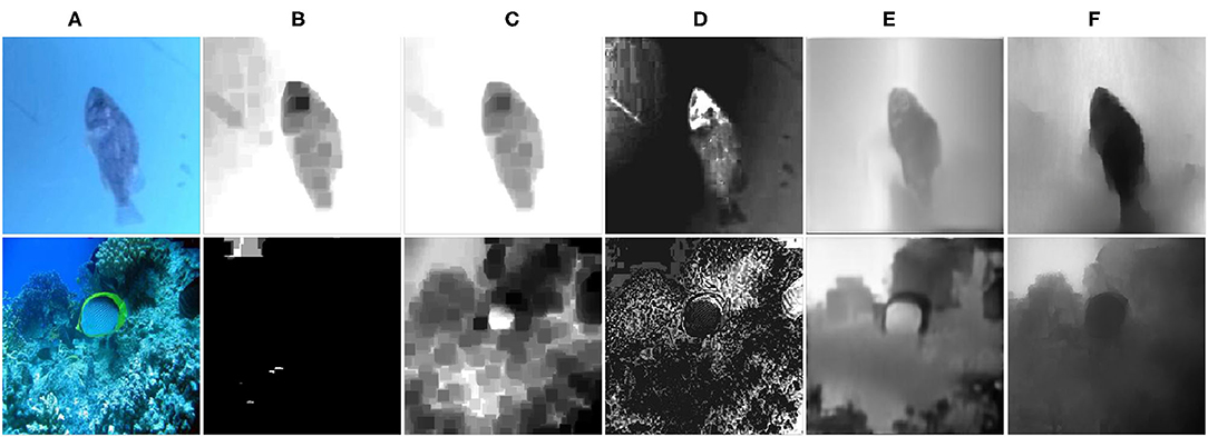
Figure 1. Examples of texture leakage during the underwater depth map estimation process using different methods. (A) Real underwater images. (B) DCP (He et al., 2010), (C) UDCP (Drews et al., 2016), (D) Berman et al. (2017), (E) UW-Net (Gupta and Mitra, 2019), (F) ours.
To address these problems, we propose a novel joint-training generative adversarial network for both multi-style underwater image synthesis and depth estimation performed in an end-to-end manner. For the former image synthetic task, we aim to transfer the hazy in-air RGB-D images to multi-style underwater images while retaining the objects and the structural information of the in-air images and controlling the underwater style through one conditional input message. To take advantage of multi-task learning (Zhang and Yang, 2017) between underwater image synthetic and depth estimation tasks, we design a joint-training generator to estimate the depth from the synthesized underwater images through full supervision. Overall, our system includes two consecutive generators (responsible for the underwater image synthesis and underwater depth estimation, separately), which are trained simultaneously. To ensure that the generated underwater images retain the objects and the structural information of the in-air images, we consider perceptual loss (Johnson et al., 2016) computed at the selected layers as a structural loss along with the adversarial loss to optimize the whole network. Furthermore, we develop a depth loss to alleviate the texture leakage phenomenon as shown in Figure 1. Finally, we evaluate the effectiveness of our proposed method to synthesize underwater images and estimate the depth map of real underwater images, and the comprehensive experimental results demonstrate the superiority of the proposed method. Overall, our main contributions of this paper are summarized as follows:
• We propose a novel joint-training generative adversarial network, which can simultaneously handle the controllable translation from the hazy RGB-D images to the multi-style realistic underwater images by combining one additional label, and the depth prediction from both the synthetic and real underwater images.
• To construct a semi-real underwater RGB-D dataset, we take the hazy in-air RGB-D image pairs and conditional labels as inputs to synthesize multi-style underwater images. During the training process, we introduce perceptual loss to preserve the objects and structural information of the in-air images during the image-to-image translation process.
• To improve the results of underwater depth estimation, we design the depth loss to make better use of high-level and low-level information. We verify the effectiveness of our proposed method on a real underwater dataset.
2. Related Work
2.1. Image-to-Image Translation
In the past several years, a series of image-to-image translation methods based on generative adversarial networks (GANs) (Mirza and Osindero, 2014; Odena et al., 2017) have been proposed. These approaches can mainly be divided into two categories of paired training and unpaired training methods. Pix2pix (Isola et al., 2017) is a typical powerful paired model and first proposes cGAN (Mirza and Osindero, 2014) learns the one-side mapping function from the input images to target images. To achieve the image-to-image translation of unpaired datasets, CycleGAN (Zhu et al., 2017a) translates images into two domains using two generators and two discriminators and proposes the cycle-consistent loss to tackle the mode collapse of unpaired image translation. To address the multimodal problem, methods including BicycleGAN (Zhu et al., 2017b), MUNIT (Huang et al., 2018), DRIT (Lee et al., 2018), StarGAN (Choi et al., 2018), etc. have been proposed. The BicycleGAN (Zhu et al., 2017b) learns to transfer the given input with a low-dimensional latent code to more diverse results. It takes advantage of the bijective consistency between the latent and target spaces to avoid the mode collapse problem. MUNIT (Huang et al., 2018) achieves multidomain translation by assuming two latent representations that present style and content, respectively and combining different representations of content and style. StarGAN (Choi et al., 2018) learns multiple mapping functions between multiple domains. It only uses a single generator and a discriminator to transfers the source images to the target domain. Then to avoid mode collapse, the generator takes the generated images and the original labels as input and transfers them to the original domain. The subsequently developed image-to-image translation methods, such as pix2pixHD (Wang et al., 2018b), GauGAN (Park et al., 2019), vid2vid (Wang et al., 2018a), FUNIT (Liu et al., 2019), NICE-GAN (Chen et al., 2020), and StarGAN v2 (Choi et al., 2020) pay more attention to generate higher visual quality, multiple outputs and have been applied in video and small sample studies.
To synthesize underwater images, due to the lack of a large paired underwater image dataset, studies have mainly focused on unsupervised learning. In a pioneering approach of underwater image synthesis, WaterGAN (Li et al., 2017) synthesized the underwater images from the in-air image and the paired depth map for real-time color correction of monocular underwater images. To achieve multidomain translation, UMGAN (Li et al., 2018) proposes an unsupervised method that combines CycleGAN (Zhu et al., 2017a) and cGAN (Mirza and Osindero, 2014) with an additional style classifier to synthesize multi-style underwater images. UW-Net developed by Gupta and Mitra (2019) learns the mapping functions between unpaired hazy RGB-D images and arbitrary underwater images to synthesize underwater images and estimate the underwater depth map. This method translates the hazy RGB-D image to underwater images while it learns to convert underwater images to the hazy RGB-D images. However, WaterGAN (Li et al., 2017) and UW-Net (Gupta and Mitra, 2019) only provide a solution for single domain underwater image generation. UMGAN (Li et al., 2018) does not consider the transmission map as an extra clue to generate underwater images. Moreover, all of the synthesized underwater images using these methods still lack the characteristics of real underwater images and clear structural information.
2.2. Underwater Depth Map Estimation
Underwater depth map estimation has mainly been studied in the field of traditional image processing. Since, He et al. (2010) first proposed a dark channel prior (DCP) for dehazing, many methods based on DCP (He et al., 2010) have been proposed for underwater depth map estimation in recent years. Drews et al. (2016) proposed a method based on a physical model of light propagation and the statistical priors of the scene to obtain the medium transmission and scene depth in typical underwater scenarios. Peng et al. (2015) proposed a three-step approach consisting of pixel blurriness estimation, rough depth map generation, and depth map refinement for depth map estimation. Berman et al. (2017) took different optical underwater types into account and proposed a more comprehensive physical image formation model to recover the distance maps and object colors. They mainly considered transmission map estimation as an intermediate step to obtain a depth map. Due to the unknown scattering parameters and multiple possible solutions, the results of these methods are most likely to be incorrect (Gupta and Mitra, 2019).
Recently, many deep learning-based methods have been proposed for depth estimation. However, most of these approaches focus on depth estimation from in-air RGB images with full supervision, which are not suitable for underwater depth map estimation due to the lack of the paired RGB-D data. The above mentioned UW-Net developed by Gupta and Mitra (2019) proposed an unsupervised method to learn depth map estimation. It considers an in-air transmission map as a cue to synthesize underwater images and obtains the required depth map from the synthesized underwater images. However, this method cannot estimate the depth map from underwater images of multiple water types. Because two competitive tasks (hazy in-air image reconstruction and depth estimation) are assigned to one generator, the depth prediction results of UW-Net lack sharp outlines. Ye et al. (2019) proposed another unsupervised adaptation networks. They developed a joint learning framework which can handle underwater depth estimation and color correction tasks simultaneously. Unlike their work, in which the two networks (style adaptation network and task network) should be trained separately, our model is more simple and can be trained simultaneously. The depth loss and a fine-tune strategy make our model more efficient in practice for underwater depth map prediction.
3. Materials and Methods
3.1. Overall Framework
In this paper, we aim to estimate the depth map from real underwater images. Because there are no paired underwater RGB-D images, we cannot perform supervised learning directly. Therefore, we choose to translate the original in-air images with corresponding depth to underwater images and obtain pseudo-paired images. To perform this task, we design an end-to-end system with two joint-training modules: multi-style underwater image synthesis and underwater depth estimation based on the synthetic paired samples. The former module is trained through unpaired training, while the latter adopts supervised training to achieve precise underwater depth estimation. The overall framework is shown in Figure 2 and consists of two generators, namely, Gs: x → ỹ and Gd: , where x and ỹ are the original in-air image and the synthesized underwater image with specific underwater style. is the estimated depth output. For discrimination, we also design two discriminators Ds and Dd to perform adversarial training to boost the underwater image synthesis and depth estimation, respectively. Ds aims to distinguish between real and fake images and identify the domains from which both the real images and the generated images originate. The discriminator Dd only learns to distinguish between the real and fake depth maps.

Figure 2. The network framework of our proposed model is designed to synthesize multi-style underwater images and estimate underwater depth maps. The generator Gs and the discriminator Ds are used to synthesize multi-style underwater images, and the generator Gd and discriminator Dd learn to estimate underwater depth map based on the synthesized underwater RGB-D dataset.
3.1.1. Multi-Style Underwater Image Synthesis
As shown in Figure 2, we refer to the training of StarGAN (Choi et al., 2018) to generate multi-style underwater images. To synthesize specified underwater style images, we adopt an additional one-hot vector c to represent domain attributes. To make the generator Gs depth-aware and preserve the original depth representation after translation, we concatenate the three inputs, namely, the in-air image (x), the target underwater style (cy), and the corresponding in-air depth (d) to synthesize an underwater image with the required style (cy), where denotes depthwise concatenation. To guarantee that the synthetic image ỹ has the target underwater style, we include an adversarial domain classifier Ds with two branches (one for domain classification and another for real/fake discrimination). The classification branch with the domain classification loss aims to recognize the underwater style (cy) of both the synthesized image ỹ and the real underwater image y. Noted that y does not have the corresponding depth annotation due to the lack of underwater ground truth. The adversarial loss is computed to promote the naturalness of the synthetic images. The generator Gs from CycleGAN (Zhu et al., 2017a) and StarGAN (Choi et al., 2018) is one symmetric encoder-decoder architecture with 6 residual blocks.
3.1.2. Underwater Depth Estimation
In the training stage, we perform underwater estimation on the above-mentioned synthetic underwater images ỹ by adopting a generator Gd with dense-block architectures. The output of generator Gs (ỹ) is the input of generator Gd used to estimate its depth map Gd(ỹ). Considering that we have the depth annotation d of the in-air images, we can obtain pseudo pairs to compute the between d and . The discriminator Dd is also designed and has only one discrimination output. Furthermore, the adversarial loss in the depth space is conducted. For underwater depth map estimation, we use DenseNet (Jégou et al., 2017) as the generator. In UW-Net (Gupta and Mitra, 2019), the authors proved the importance of using hazy above-water images and compared the results of underwater depth maps estimation with different generator networks, including ResNet (He et al., 2016), Unet (Ronneberger et al., 2015), DenseNet (Jégou et al., 2017), and so on. In their work, DenseNet is proved to be the best choice.
3.2. Loss Functions
3.2.1. Multi-Style Underwater Image Synthesis
3.2.1.1. Adversarial Loss
Regular GANs use sigmoid activation output and the cross-entropy loss function (Goodfellow et al., 2014), which may cause a vanishing gradient during the learning process. To stabilize the training process and generate underwater images with higher quality, we adapt the least-squares loss (Mao et al., 2017) in our method. can be expressed as follows:
where Gs targets the transfer of a hazy in-air RGB-D image x by concatenating an underwater condition label cy to synthesize image . The discriminator Ds attempts to distinguish the real underwater image y and the synthesized underwater image ỹ.
3.2.1.2. Domain Classification Loss
For the given hazy in-air image x and an underwater domain style cy, Gs translates x into an underwater image ỹ, which can be properly classified to the desired target domain by Ds. To achieve this goal, the classification branch of Ds imposes the domain classification. For the real underwater image y, the domain classification loss is computed as:
where the term Ds(cy|y) denotes a probability distribution over the underwater domain labels (cy) computed by Ds. By minimizing this objective, Ds learns to classify an underwater image y to its original domain cy. We assume that the underwater image and domain label pair (y, cy) is given by the training data. For generator Gs, the loss function for the domain classification of synthetic underwater images is defined as:
During the training, Gs tries to synthesize underwater image ỹ that can fool the classification branch of Ds.
3.2.1.3. Feature-Level Loss
Beyond the pixel-level loss, we design feature-level loss functions between the feature representations extracted from a pre-trained VGG19 network. The hybrid feature-level loss can effectively preserve the similarity of the object between the hazy in-air images and the synthesized underwater images. For the multi-style underwater image synthesis, we introduce a perceptual loss, namely, . is designed to preserve the object content and loosen the restrictions on the color and textile changes after translation. is expressed as follows:
where Φ(i) denotes the parameters at the i-th layer of a pre-trained VGG19 network. Following the work by Kupyn et al. (2019), we compute the 1-norm distance at the same selected i = 14 layer of the VGG19 network between the hazy in-air images and the synthesized underwater images.
3.2.1.4. Reconstruction Loss
To perform unpaired training between in-air and underwater images, we include the cycle consistency loss (Zhu et al., 2017a) in our framework. The reconstruction loss between and x is defined as follows:
where cx and cy indicate the original hazy in-air domain label and the target underwater domain style, respectively. Gs takes the counterpart Gs(x|cy), its corresponding depth, and the original domain label cx as input and tries to reconstruct the original hazy in-air image. We adapt the L1 loss as our reconstruction loss. Note that we use the generator Gs twice, first to translate the hazy in-air RGB-D images into an underwater image in the target domain and then to reconstruct the hazy in-air RGB images from the translated images.
3.2.2. Underwater Depth Estimation
3.2.2.1. Adversarial Loss
For the second underwater depth estimation procedure, the adversarial loss is described as:
where Gd learns the mapping function from the synthesized underwater images ỹ to the in-air depth d as Gd(ỹ) → d. Dd is responsible to recognize the fake ingredient from the synthesized depth output .
3.2.2.2. Depth Loss
For underwater depth estimation, the pixel-level distance between the estimated value and the ground truth, such as 1-norm and 2-norm, is generally adopted to favor less blurring. However, we find that only the pixel-level loss between the predicted depth map and the ground truth often leads to poor performance due to the influences of noise, water with various turbidity, etc (Please refer to section 4.3 for more details). To force the model to pay more attention to the objects, we make use of the feature representations extracted from a pre-trained VGG19 network for multi-level information. We also introduce pixel-level distance for low-level details. Finally, to obtain improved results, we combine 1-norm loss and the multi-layer feature constraint between and d and define the depth loss, namely :
Similarly, Φ(i) represents the pre-trained parameter of the i-th layer. Here, following the work of Wang et al. (2018b) and Wang C. et al. (2018), we compute the L1 distance at the same selected six layers: i = 1, 6, 11, 20, 29.
3.3. Full Objective
Finally, the objective functions can be written, respectively, as:
where α, γ, λ, and η are the hyperparameters that control the effect of each loss in the final objective function. We set α = 5, γ = 10, λ = 0.1, η = 50 in all of our experiments, and we optimize the objective function with the Adam optimizer (Kingma and Ba, 2015). To choose appropriate weights, we design ablation studies for each hyperparameter except for γ. We follow StarGAN (Choi et al., 2018) to set γ = 10. For the choice of the rest of hyperparameters, please refer to section 4.3 for more details.
4. Results
4.1. Datasets and Implementation Details
In our experiments, we translate the hazy in-air images to two underwater domains (green and blue). We also choose the hazy in-air D-Hazy dataset (Ancuti et al., 2016) as the input images; this dataset contains the indoor scenes. For the two underwater domains, we adapt the real underwater images from the SUN (Xiao et al., 2010), URPC,1 EUVP (Islam et al., 2020), UIEB (Li et al., 2019), and Fish datasets.2 We collect 1,031 blue and 1,004 green underwater images from these datasets and the Google website, respectively. The D-Hazy dataset (Ancuti et al., 2016) includes 1,449 images. We randomly choose 1,300 images as the in-air images x to train the model. The remaining 149 images of the dataset are selected for evaluation. We use random-crop to obtain 128 × 128 patches for training. For the evaluation stage, we take complete images of 256 × 256. The entire network is trained on one Nvidia GeForce GTX 1070 using the Pytorch framework. To avoid the mode collapse problem, we apply spectral normalization (Miyato et al., 2018) in both the discriminators and the generators. Because of the introduction of spectral normalization (Miyato et al., 2018), we use a two-timescale update rule (TTUR) based on BigGAN (Brock et al., 2019) and SAGAN (Zhang et al., 2018). The Adam algorithm is applied with a learning rate of 0.0002 for the discriminators while 0.00005 for the generators. Because of the limited computing resources, we set the batch size to 10 and perform 100,000 training iterations in our experiments.
4.2. Comparison Methods
Our method achieves underwater depth map estimation using multi-style synthesized underwater images. In this section, we first evaluate the performance of WaterGAN (Li et al., 2017), CycleGAN (Zhu et al., 2017a), StarGAN (Choi et al., 2018), UW-Net (Gupta and Mitra, 2019), StarGAN v2 (Choi et al., 2020), and our method on multiple synthetic underwater images. Additionally, to evaluate the effectiveness of underwater depth map estimation, we compare the results obtained using DCP (He et al., 2010), UDCP (Drews et al., 2016), Berman et al. (2017), Gupta and Mitra (2019), and our method.
4.2.1. Qualitative Evaluation
To evaluate the effectiveness of the proposed method, we perform underwater image synthesis on the NYUv2 (Silberman et al., 2012) and D-Hazy (Ancuti et al., 2016) datasets. Figure 3 shows a visual comparison of the synthesized underwater images generated by different methods. WaterGAN (Li et al., 2017) takes advantage of in-air RGB-D images to synthesize underwater images. As shown in Figure 3B, the results are somewhat single-hued and lack water characteristics. Although WaterGAN supports multi-style image generation, the two styles (blue and green) obtained by WaterGAN in Figure 3B are difficult to distinguish. The results of CycleGAN (Zhu et al., 2017a) retain most of the contents and structures of the original images. Compared to WaterGAN, they are similar to the natural underwater scenes shown in Figure 3C. By contrast, the outputs of CycleGAN (Zhu et al., 2017a) include serious distortions of the details of the image with incorrect depth information. StarGAN (Choi et al., 2018) can simultaneously translate in-air images into multiple underwater styles. However, the results lack the characteristics of real underwater images, such as depth information, and clear structural information of the objects. Besides, many artifacts are observed in Figure 3D. UW-Net (Gupta and Mitra, 2019) also takes hazy in-air RGB-D images as input, the results are presented in Figure 3E and show fuzzy structures for the objects. The results of StarGAN v2 (Choi et al., 2020) are shown in Figure 3F. There is no denying that StarGAN v2 (Choi et al., 2020) possesses a powerful style network to extract style codes from reference images. However, the underwater images provided by StarGAN v2 fail to help the depth estimation tasks. As shown in Figure 3F, StarGAN v2 removed some objects and structural information during the image synthetic process, which makes the synthetic underwater images and their corresponding in-air depth maps unmatched. The quantitative results in section 4.2.2 further confirm this point.
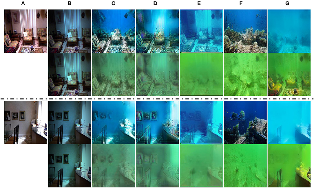
Figure 3. Comparison of the visual quality of synthesized underwater images obtained by different methods. From left to right, (A) are original in-air images, (B–G) are the results of the WaterGAN (Li et al., 2017), CycleGAN (Zhu et al., 2017a), StarGAN (Choi et al., 2018), UW-Net (Gupta and Mitra, 2019), StarGAN v2 (Choi et al., 2020), and our method.
Our model is optimized to synthesize underwater images with multiple styles based on the unpaired datasets. The results of our method (Figure 3G), in which the structural information is well preserved, are better than those obtained from other methods in terms of visual quality.
For underwater depth map estimation, Figure 4 shows the results of our method and other methods developed by He et al. (2010) (DCP), (Drews et al., 2016) (UDCP), Berman et al. (2017), and Gupta and Mitra (2019) based on the underwater images obtained by Berman et al. (2017). In Figures 4B–D, these methods fail to capture relative depth of the scene with respect to the camera. Moreover, these methods mainly obtain the transmission maps of the scene and have excessive texture leakage in the results. Gupta and Mitra (2019) used an unsupervised method to estimate the depth map, obtaining the results shown in Figure 4E, and this method appears to be better than the other methods, whose results are presented in Figures 4B–D. However, this method still suffers from excessive texture leakage and only estimates the depth map for single-domain underwater images. Our results have a much more reasonable appearance with a linear depth variation. On the other hand, we observe that our network successfully captures the depth information from multi-style underwater images. More results for real underwater images with different underwater characteristics are seen in Figure 5. Furthermore, the UW-Net (Gupta and Mitra, 2019) and our method synthesize underwater images using the underwater dataset provided by Berman et al. (2017) to fine-tune the models of the depth map estimation. We fine-tune our model for 10,000 iterations on Berman et al.'s dataset for better depth map estimation.

Figure 4. Comparison of our method with other underwater depth estimation methods. From left to right, (A) are real underwater images from the dataset of Berman et al. (2017), (B–F) are the results of DCP (He et al., 2010), UDCP (Drews et al., 2016), Berman et al. (2017), Gupta and Mitra (2019), and our method, and (G) are the ground truths.
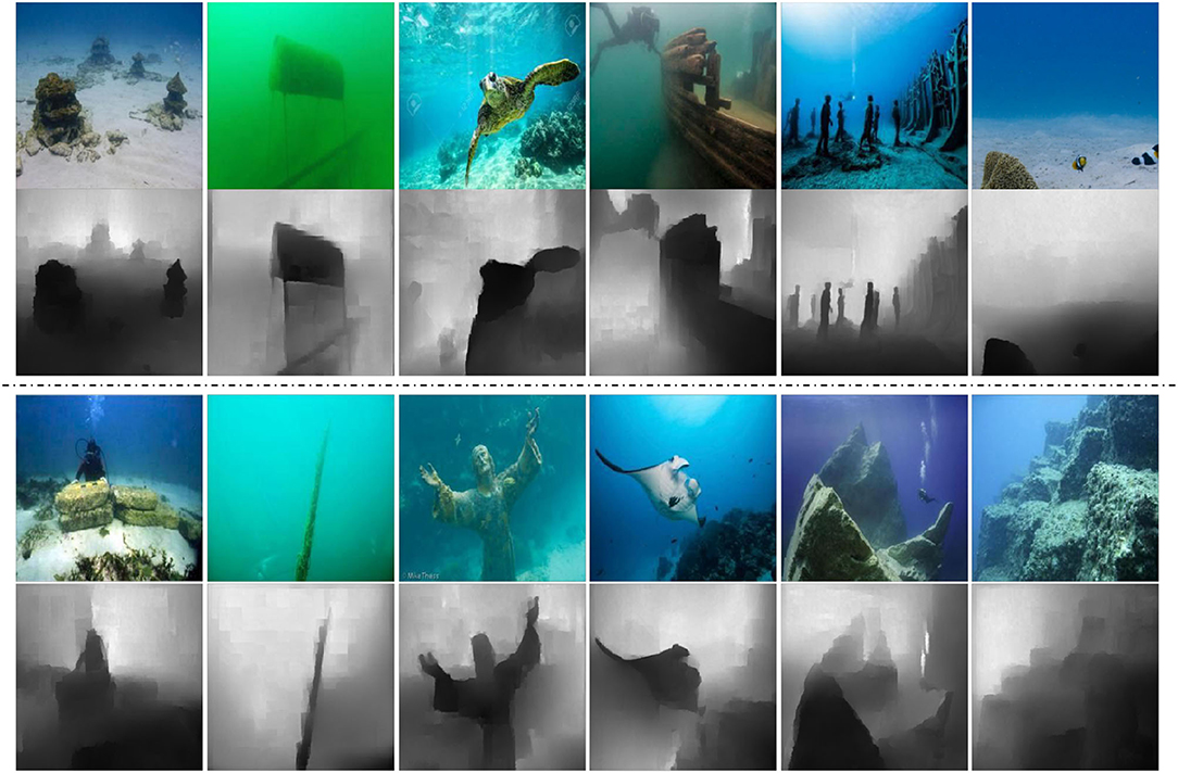
Figure 5. The results of our model for depth map estimation. Every two rows from top to bottom are real underwater images with different illumination and scattering conditions and the results of our model for depth map estimation.
4.2.2. Quantitative Evaluation
The dataset of Berman et al. (2017) consists of 114 paired underwater RGB-D images from Katzaa, Michmoret, Nachsholim, and Satil. We use 71 images belonging to the three regions Katzaa, Nachsholim, and Satil. Because the Michmoret region has very few natural objects and is of the same scene. Following UW-Net (Gupta and Mitra, 2019), we use two metrics for comparison, namely, log scale-invariant mean squared error (SI-MSE) (Eigen et al., 2014) and the Pearson correlation coefficient (ρ). Considering the fact that the depth map provided by the stereo camera is not complete (e.g., the ground truth of the white regions in Figure 7H are not provided), we only calculate the pixels with a defined depth-value in the ground truth (GT).
The underwater image synthesis assists to estimate depth maps from real underwater images. Thus, how much the synthetic underwater images can be used to boost the performance of underwater image-based depth prediction is the key evaluation index. We evaluate performance on depth prediction tasks with a series of the state-of-the-art methods, which consist of WaterGAN (Li et al., 2017), CycleGAN (Zhu et al., 2017a), StarGAN (Choi et al., 2018), UW-Net (Gupta and Mitra, 2019), and StarGAN v2 (Choi et al., 2020). We aim to calculate the depth map estimation results on a semi-real underwater RGB-D dataset. UW-Net suggests that fine-tuning the models with a few unlabeled images from the target underwater environment could further boost the depth prediction performance. During the fine-tuning process, we only use the RGB underwater images without considering the depth ground truth of the data from Berman et al. to show the ability that our model can adapt itself to a new environment well. To make it fair, we fine-tune all models to generate a similar underwater style of the dataset of Berman et al..
Although our model already provides a solution for a depth estimation task, we choose a typical independent supervised image-to-image model, pix2pix (Isola et al., 2017), to fairly evaluate the potential of synthetic underwater images on the application of depth prediction. We use identical pix2pix models to learn the mapping function between the generate underwater images of different underwater image synthetic methods and their corresponding in-air depth maps. Finally, we test and evaluate all models on the dataset of Berman et al.. Table 1 shows the results, and our model obtains higher ρ values and lower SI-MSE.

Table 1. Quantitative comparison of our method and other methods for underwater image synthesis.
For the underwater depth estimation task, Table 2 shows the quantitative results. Our method obtains the least scale-invariant error (SI-MSE) (Eigen et al., 2014) and the highest Pearson correlation coefficient (ρ).
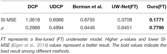
Table 2. Quantitative comparison of our method and other methods on the dataset of Berman et al. (2017).
We also investigate the parameters and Floating Point Operations (Tan and Le, 2019) (FLOPs) among different generators in Table 3. In the case of CycleGAN, we only count the FLOPs and parameters of a single generator. We can find that the proposed method can achieve better performance with fewer network parameters and computational cost. Benefiting from the dense blocks, the Gd of our model has fewer parameters and FLOPs than Gs. Please note that Gs is only used in training stage. In testing phase, we only need Gd to estimate the depth map.
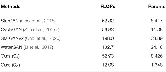
Table 3. Comparison of Floating Point Operations (FLOPs) and total number of parameters among different generators with a size of 256 × 256.
4.3. Ablation Study
4.3.1. Loss Selection of Underwater Image Synthesis
To preserve clear structural information, we consider the perceptual loss , structural similarity index (SSIM) , and multiscale structural similarity index (MS-SSIM) as the structural loss. We evaluate the efficiency of each loss, including , , and , and based on the visual effect of the synthesized underwater images and the results of depth map estimation, we choose the perceptual loss. To verify the effectiveness of the extra losses in our network, we design ablation experiments and perform a comparison on D-Hazy (Ancuti et al., 2016) which consists of 1,449 images. Figure 6 shows that each loss affects the quality of the generated underwater images. It is observed from Figure 6B, that the generated underwater images using ResNet without any extra loss have more color blocks and artifacts. Additionally, during the training, it is extremely unstable and tends to produce color inversions and serious distortions situations. In Figures 6C,D, many artifacts are still retained for ResNet with or . Table 4 shows the results of depth map estimation based on different synthetic underwater image datasets, which are generated by ResNet and ResNet with extra losses, separately. Using , we obtain the best results of underwater depth map estimation. Based on the experiments mentioned above, we introduce a perceptual loss to preserve the details and restrain the artifacts in Figure 6E. To minimize the negative effects of the synthesized images, we design experiments to determine the proper weight of α and λ. In Table 5, we show the results of different weights, including α and λ. We note that both UW-Net and our model can be fine-tuned on the dataset of Berman et al. to obtain better results of underwater depth map estimation. Fine-tuning processing provides a flexible approach for adjusting our model and the estimation of depth maps from unexplored underwater regions within a relatively short period.
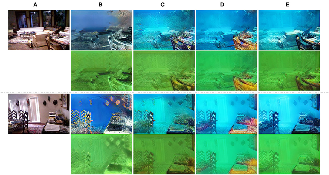
Figure 6. Sample results of our method for synthesizing underwater images using different losses. , and , respectively represent SSIM loss, MS-SSIM loss, and perceptual loss. (A) Are in-air images, (B) are the results without any structural loss (Baseline), (C–E) are the results with , , and , respectively.

Table 4. Comparison of our method for the synthesis of underwater images with different combinations.
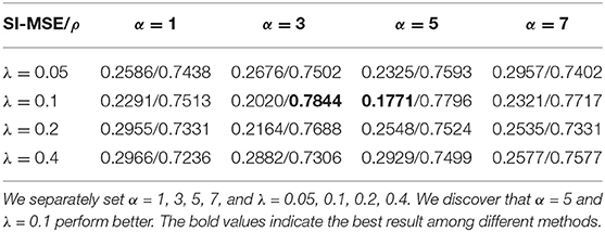
Table 5. Comparison of weights used in the objective function of our model, including α and λ.
4.3.2. The Design of Underwater Depth Map Estimation
With the support of synthetic paired RGB-D data, we consider L1 loss, L2 loss, Lssim loss, or Lmsssim loss to learn the mapping functions for supervised depth map prediction. During the training, we observe the all above-mentioned losses are not enough to generate more correct depth maps. The results in Figures 7B–E show that depth prediction based on the above-mentioned losses are easily affected by the shape, noise, etc. As mentioned in section 3.2.2, we design depth loss Ldepth to make better use of low-level and high-level feature information and avoid the risk of texture leakage. We take advantage of a pre-trained VGG19 network to extract feature maps between the generated depth maps and the ground truths. We assume the feature maps between the generated depth map and its corresponding ground truth in each layer from a pre-trained VGG19 network should be equal. The loss Ldepth makes our model pay more attention to the objects and the relative distance in the underwater images. Inspired by Wang et al.'s work (Wang C. et al., 2018), we also attempt to extract feature maps from the discriminator Dd, namely , rather than a pre-trained VGG19 network. In Figure 7F, we can see that our model with are often overwhelmed with incorrect boundary prediction due to the insufficient layers of our discriminator Dd to extract high-level feature maps comparing with . Furthermore, we investigate the optimal parameter setting of η with a greedily searching strategy (Table 6), and we discover that η = 50 is the best choice among all the parameters.
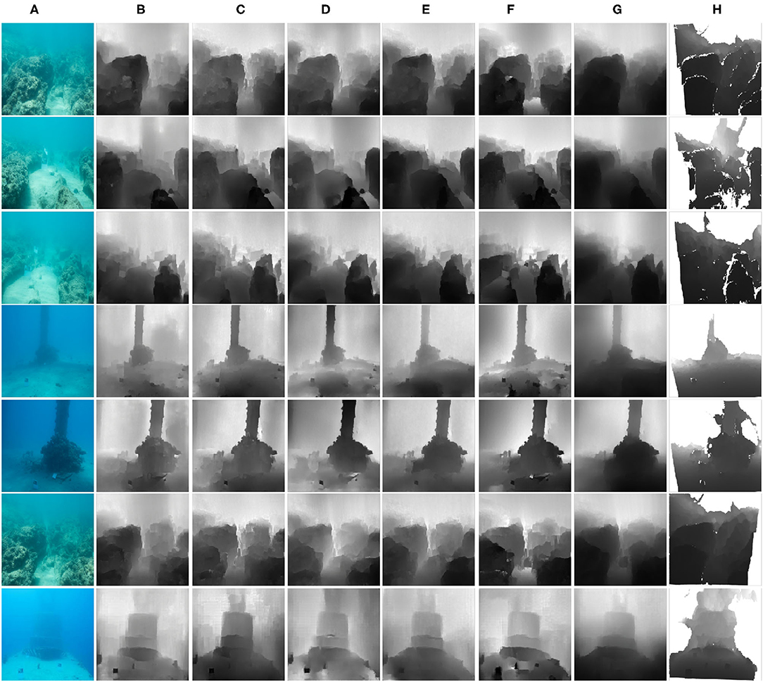
Figure 7. Effectiveness evaluation of the , , , , and . From left to right, respectively, (A) are real underwater images, (B–H) are the results of depth map estimation with L1 loss, L2 loss, , , , , and their corresponding ground truths.
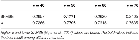
Table 6. Results with different η values.
Based on Figure 7 and Table 7, we can easily conclude that the results of depth map estimation using Ldepth loss are more accurate and continuous. The results show sharper outlines. We can clearly distinguish the relative distance and the objects.

Table 7. Quantitative comparison of our method with different losses on the dataset of Berman et al. (2017).
5. Discussions and Conclusion
To further explore the potential of our model on depth prediction, we considered the work by Li et al. (2018) and prepared a more complex underwater image dataset including four different styles. In this experiment, we still consider the depth map as a conditional input to synthesize a corresponding underwater image. But we did not utilize the physical parameters (e.g., the water turbidity or any optical parameters) for the unpaired image-to-image translation. Instead, we roughly divide the images with different water turbidity into four groups and follow the manner of StarGAN (Choi et al., 2018) to perform conditional image translation. Some synthetic examples of four different styles are shown in Figure 8. Due to the lack of ground truth of the depth map, we cannot quantitatively evaluate the effectiveness of our model for multi-style underwater depth map estimation. Instead, we prepared several qualitative evaluation results, as shown in Figure 9. Intuitively, we find that the depth estimation of a side-view underwater image is better than that from a vertical view. This result is caused by the lack of vertical view in-air images from the in-air D-Hazy dataset required to produce sufficient synthetic underwater vertical view images. We plan to improve the performance on this point by data augmentation in the future.
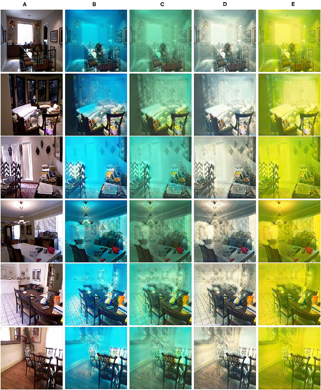
Figure 8. Sample results for the synthesis of underwater images. (A) Show in-air images. (B–E) Represent blue style, green style, white style and yellow style, respectively.
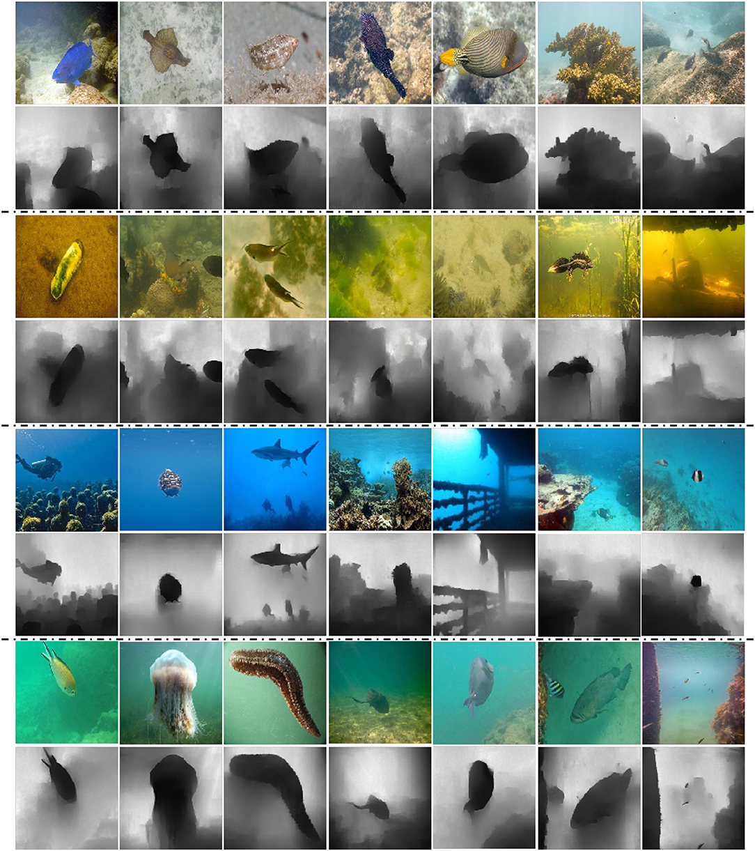
Figure 9. Multi-style underwater depth map estimation. The rows from top to bottom are real underwater images with four different water types and the results of our model for depth map estimation. Every two rows are real underwater images and their predicted depth maps of our method.
In this paper, we proposed an end-to-end system that can synthesize multi-style underwater images using one-hot encoding and estimate underwater depth maps. The system can convert the in-air RGB-D images into more realistic underwater images with multiple watercolor styles. Then we use the synthesized underwater RGB images to construct a semi-real underwater RGB-D dataset. With the synthetic underwater RGB-D dataset, our model can learn to estimate underwater depth maps using supervised learning. Finally, we compare our method with existing state-of-the-art methods to synthesize underwater images and estimate underwater depth maps, and we verify that our method outperforms these methods both qualitatively and quantitatively. Furthermore, our model can be fine-tuned on the untrained datasets to synthesize a similar underwater style. It effectively makes our model to be applied for depth map estimation on new underwater datasets.
Data Availability Statement
The raw data supporting the conclusions of this article will be made available by the authors, without undue reservation.
Author Contributions
QZ performed the experiments and wrote the manuscript. ZZ and HZe revised the manuscript. ZY provided the ideas and revised the article. HZh and BZ provided advices and GPU devices for parallel computing. All authors contributed to the article and approved the submitted version.
Funding
This work was supported by the finance science and technology project of 630 Hainan province of China under Grant Number ZDKJ202017 and National Natural Science Foundation of China under Grant Numbers 62171419 and 61701463.
Conflict of Interest
The authors declare that the research was conducted in the absence of any commercial or financial relationships that could be construed as a potential conflict of interest.
Publisher's Note
All claims expressed in this article are solely those of the authors and do not necessarily represent those of their affiliated organizations, or those of the publisher, the editors and the reviewers. Any product that may be evaluated in this article, or claim that may be made by its manufacturer, is not guaranteed or endorsed by the publisher.
Footnotes
References
Abas, P. E., and De Silva, L. C. (2019). Review of underwater image restoration algorithms. IET Image Process. 13, 1587–1596. doi: 10.1049/iet-ipr.2019.0117
Akkaynak, D., and Treibitz, T. (2019). “Sea-thru: a method for removing water from underwater images,” in Proceedings of the IEEE/CVF Conference on Computer Vision and Pattern Recognition (Long Beach, CA: Computer Vision Foundation; IEEE), 1682–1691. doi: 10.1109/CVPR.2019.00178
Ancuti, C., Ancuti, C. O., and De Vleeschouwer, C. (2016). “D-hazy: a dataset to evaluate quantitatively dehazing algorithms,” in IEEE International Conference on Image Processing (IEEE), 2226–2230. doi: 10.1109/ICIP.2016.7532754
Berman, D., Levy, D., Avidan, S., and Treibitz, T. (2020). Underwater single image color restoration using haze-lines and a new quantitative dataset. IEEE Trans. Pattern Anal. Mach. Intell. 43, 2822–2837. doi: 10.1109/TPAMI.2020.2977624
Berman, D., Treibitz, T., and Avidan, S. (2017). “Diving into haze-lines: color restoration of underwater images,” in Proceedings of the British Machine Vision Conference (BMVA Press).
Brock, A., Donahue, J., and Simonyan, K. (2019). “Large scale GAN training for high fidelity natural image synthesis,” in Proceedings of the 7th International Conference on Learning Representations, ICLR 2019 (New Orleans, LA).
Chen, R., Huang, W., Huang, B., Sun, F., and Fang, B. (2020). “Reusing discriminators for encoding: towards unsupervised image-to-image translation,” in Proceedings of the IEEE/CVF Conference on Computer Vision and Pattern Recognition (Seattle, WA: IEEE), 8168–8177. doi: 10.1109/CVPR42600.2020.00819
Choi, Y., Choi, M., Kim, M., Ha, J.-W., Kim, S., and Choo, J. (2018). “Stargan: unified generative adversarial networks for multi-domain image-to-image translation,” in IEEE Conference on Computer Vision and Pattern Recognition (Salt Lake City, UT: IEEE Computer Society), 8789–8797. doi: 10.1109/CVPR.2018.00916
Choi, Y., Uh, Y., Yoo, J., and Ha, J.-W. (2020). “Stargan v2: diverse image synthesis for multiple domains,” in Proceedings of the IEEE/CVF Conference on Computer Vision and Pattern Recognition (Salt Lake City, UT: IEEE), 8188–8197. doi: 10.1109/CVPR42600.2020.00821
Churnside, J. H., Marchbanks, R. D., Lembke, C., and Beckler, J. (2017). Optical backscattering measured by airborne lidar and underwater glider. Remote Sens. 9:379. doi: 10.3390/rs9040379
Dancu, A., Fourgeaud, M., Franjcic, Z., and Avetisyan, R. (2014). “Underwater reconstruction using depth sensors,” in Special Interest Group Graph. Interact. Techn (Association for Computing Machinery), 1–4. doi: 10.1145/2669024.2669042
Deris, A., Trigonis, I., Aravanis, A., and Stathopoulou, E. (2017). Depth cameras on UAVs: a first approach. Int. Arch. Photogr. Remote Sens. Spat. Inform. Sci. 42:231. doi: 10.5194/isprs-archives-XLII-2-W3-231-2017
Drews, P. L., Nascimento, E. R., Botelho, S. S., and Campos, M. F. M. (2016). Underwater depth estimation and image restoration based on single images. IEEE Comput. Graph. Appl. 36, 24–35. doi: 10.1109/MCG.2016.26
Eigen, D., Puhrsch, C., and Fergus, R. (2014). “Depth map prediction from a single image using a multi-scale deep network,” in Advances in Neural Information Processing Systems (Montreal, QC), 2366–2374.
Gomez Chavez, A., Ranieri, A., Chiarella, D., Zereik, E., Babić, A., and Birk, A. (2019). Caddy underwater stereo-vision dataset for human-robot interaction (HRI) in the context of diver activities. J. Mar. Sci. Eng. 7:16. doi: 10.3390/jmse7010016
Goodfellow, I., Pouget-Abadie, J., Mirza, M., Xu, B., Warde-Farley, D., Ozair, S., et al. (2014). “Generative adversarial nets,” in Advances in Neural Information Processing Systems, eds Z. Ghahramani, M. Welling, C. Cortes, N. D. Lawrence, and K. Q. Weinberger (Montreal, QC), 2672–2680.
Gupta, H., and Mitra, K. (2019). “Unsupervised single image underwater depth estimation,” in IEEE International Conference on Image Processing (IEEE), 624–628. doi: 10.1109/ICIP.2019.8804200
He, K., Sun, J., and Tang, X. (2010). “Single image haze removal using dark channel prior”, 2009 IEEE Computer Society Conference on Computer Vision and Pattern Recognition (CVPR 2009) (Miami, FL: IEEE Computer Society), 1956–1963.
He, K., Zhang, X., Ren, S., and Sun, J. (2016). “Deep residual learning for image recognition,” in Proceedings of the IEEE Conference on Computer Vision and Pattern Recognition (Las Vegas, NV), 770–778. doi: 10.1109/CVPR.2016.90
Huang, X., Liu, M.-Y., Belongie, S., and Kautz, J. (2018). “Multimodal unsupervised image-to-image translation,” in Proceedings of the European Conference on Computer Vision (ECCV), 172–189. doi: 10.1007/978-3-030-01219-9_11
Islam, M. J., Xia, Y., and Sattar, J. (2020). Fast underwater image enhancement for improved visual perception. IEEE Robot. Autom. Lett. 5, 3227–3234. doi: 10.1109/LRA.2020.2974710
Isola, P., Zhu, J.-Y., Zhou, T., and Efros, A. A. (2017). “Image-to-image translation with conditional adversarial networks,” in IEEE Conference on Computer Vision and Pattern Recognition (Honolulu, HI: IEEE Computer Society), 1125–1134. doi: 10.1109/CVPR.2017.632
Jégou, S., Drozdzal, M., Vazquez, D., Romero, A., and Bengio, Y. (2017). “The one hundred layers tiramisu: fully convolutional densenets for semantic segmentation,” in Proceedings of the IEEE Conference on Computer Vision and Pattern Recognition, 11–19. doi: 10.1109/CVPRW.2017.156
Johnson, J., Alahi, A., and Fei-Fei, L. (2016). “Perceptual losses for real-time style transfer and super-resolution,” in European Conference on Computer Vision, 694–711. doi: 10.1007/978-3-319-46475-6_43
Kingma, D. P., and Ba, J. (2015). “Adam: a method for stochastic optimization,” in Proceedings of the 3rd International Conference on Learning Representations, eds. Y. Bengio and Y. LeCun (San Diego, CA).
Kupyn, O., Martyniuk, T., Wu, J., and Wang, Z. (2019). “Deblurgan-v2: Deblurring (orders-of-magnitude) faster and better,” in Proceedings of the IEEE International Conference on Computer Vision (Seoul: IEEE), 8878–8887. doi: 10.1109/ICCV.2019.00897
Lee, H.-Y., Tseng, H.-Y., Huang, J.-B., Singh, M., and Yang, M.-H. (2018). “Diverse image-to-image translation via disentangled representations,” in Proceedings of the European Conference on Computer Vision (ECCV), 35–51. doi: 10.1007/978-3-030-01246-5_3
Li, C., Guo, C., Ren, W., Cong, R., Hou, J., Kwong, S., et al. (2019). An underwater image enhancement benchmark dataset and beyond. IEEE Trans. Image Process. 29, 4376–4389. doi: 10.1109/TIP.2019.2955241
Li, J., Skinner, K. A., Eustice, R., and Johnson-Roberson, M. (2017). WaterGAN: unsupervised generative network to enable real-time color correction of monocular underwater images. IEEE Robot. Autom. Lett. 3, 387–394. doi: 10.1109/LRA.2017.2730363
Li, N., Zheng, Z., Zhang, S., Yu, Z., Zheng, H., and Zheng, B. (2018). The synthesis of unpaired underwater images using a multistyle generative adversarial network. IEEE Access 6, 54241–54257. doi: 10.1109/ACCESS.2018.2870854
Liu, M.-Y., Huang, X., Mallya, A., Karras, T., Aila, T., Lehtinen, J., et al. (2019). “Few-shot unsupervised image-to-image translation,” in Proceedings of the IEEE International Conference on Computer Vision (Seoul: IEEE), 10551–10560. doi: 10.1109/ICCV.2019.01065
Mao, X., Li, Q., Xie, H., Lau, R. Y., Wang, Z., and Paul Smolley, S. (2017). “Least squares generative adversarial networks,” in IEEE Conference on Computer Vision and Pattern Recognition (Venice: IEEE Computer Society), 2813–2821. doi: 10.1109/ICCV.2017.304
Massot-Campos, M., and Oliver-Codina, G. (2015). Optical sensors and methods for underwater 3d reconstruction. Sensors 15, 31525–31557. doi: 10.3390/s151229864
Mirza, M., and Osindero, S. (2014). Conditional generative adversarial nets. arXiv preprint arXiv:1411.1784.
Miyato, T., Kataoka, T., Koyama, M., and Yoshida, Y. (2018). Spectral normalization for generative adversarial networks. arXiv preprint arXiv:1802.05957.
Odena, A., Olah, C., and Shlens, J. (2017). “Conditional image synthesis with auxiliary classifier GANs,” in International Conference on Machine Learning, eds D. Precup and Y. W. Teh (Sydney, NSW: PMLR), 2642–2651.
Park, T., Liu, M.-Y., Wang, T.-C., and Zhu, J.-Y. (2019). “Semantic image synthesis with spatially-adaptive normalization,” in Proceedings of the IEEE/CVF Conference on Computer Vision and Pattern Recognition (Long Beach, CA: Computer Vision Foundation; IEEE), 2337–2346. doi: 10.1109/CVPR.2019.00244
Peng, Y.-T., Zhao, X., and Cosman, P. C. (2015). “Single underwater image enhancement using depth estimation based on blurriness,” in IEEE International Conference on Image Processing (IEEE), 4952–4956. doi: 10.1109/ICIP.2015.7351749
Pérez, J., Bryson, M., Williams, S. B., and Sanz, P. J. (2020). Recovering depth from still images for underwater dehazing using deep learning. Sensors 20:4580. doi: 10.3390/s20164580
Ronneberger, O., Fischer, P., and Brox, T. (2015). “U-net: convolutional networks for biomedical image segmentation,” in International Conference on Medical Image Computing and Computer Assisted Intervention (Springer), 234–241. doi: 10.1007/978-3-319-24574-4_28
Silberman, N., Hoiem, D., Kohli, P., and Fergus, R. (2012). “Indoor segmentation and support inference from RGBD images,” in European Conference on Computer Vision (Springer), 746–760. doi: 10.1007/978-3-642-33715-4_54
Tan, M., and Le, Q. (2019). “Efficientnet: Rethinking model scaling for convolutional neural networks,” in International Conference on Machine Learning (PMLR), 6105–6114.
Ueda, T., Yamada, K., and Tanaka, Y. (2019). “Underwater image synthesis from rgb-d images and its application to deep underwater image restoration,” in 2019 IEEE International Conference on Image Processing (ICIP) (IEEE), 2115–2119. doi: 10.1109/ICIP.2019.8803195
Wang, C., Xu, C., Wang, C., and Tao, D. (2018). Perceptual adversarial networks for image-to-image transformation. IEEE Trans. Image Process. 27, 4066–4079. doi: 10.1109/TIP.2018.2836316
Wang, T.-C., Liu, M.-Y., Zhu, J.-Y., Liu, G., Tao, A., Kautz, J., et al. (2018a). “Video-to-video synthesis,” in Advances in Neural Information Processing Systems 31: Annual Conference on Neural Information Processing Systems 2018, eds S. Bengio, H. M. Wallach, H. Larochelle, K. Grauman, N. Cesa-Bianchi, and R. Garnett (Montreal, QC), 1152–1164.
Wang, T.-C., Liu, M.-Y., Zhu, J.-Y., Tao, A., Kautz, J., and Catanzaro, B. (2018b). “High-resolution image synthesis and semantic manipulation with conditional GANs,” in Proceedings of the IEEE Conference on Computer Vision and Pattern Recognition (Salt Lake City, UT: IEEE Computer Society), 8798–8807. doi: 10.1109/CVPR.2018.00917
Xiao, J., Hays, J., Ehinger, K. A., Oliva, A., and Torralba, A. (2010). “Sun database: Large-scale scene recognition from abbey to zoo,” in IEEE Conference on Computer Vision and Pattern Recognition (San Francisco, CA: IEEE Computer Society), 3485–3492. doi: 10.1109/CVPR.2010.5539970
Ye, X., Li, Z., Sun, B., Wang, Z., Xu, R., Li, H., et al. (2019). Deep joint depth estimation and color correction from monocular underwater images based on unsupervised adaptation networks. IEEE Trans. Circ. Syst. Video Technol. 30, 3995–4008. doi: 10.1109/TCSVT.2019.2958950
Zhang, H., Goodfellow, I., Metaxas, D., and Odena, A. (2018). “Self-attention generative adversarial networks,” in Proceedings of the 36th International Conference on Machine Learning, eds K. Chaudhuri and R. Salakhutdinov (Long Beach, CA: PMLR), 7354–7363.
Zheng, Z., Wu, Y., Han, X., and Shi, J. (2020). “ForkGAN: seeing into the rainy night,” in Computer Vision-ECCV 2020: 16th European Conference (Glasgow: Springer), 155-170. doi: 10.1007/978-3-030-58580-8_10
Zhu, J.-Y., Park, T., Isola, P., and Efros, A. A. (2017a). “Unpaired image-to-image translation using cycle-consistent adversarial networks,” in IEEE Conference on Computer Vision and Pattern Recognition (Venice: IEEE Computer Society), 2223–2232. doi: 10.1109/ICCV.2017.244
Zhu, J.-Y., Zhang, R., Pathak, D., Darrell, T., Efros, A. A., Wang, O., et al. (2017b). “Toward multimodal image-to-image translation,” in Advances in Neural Information Processing Systems, eds I. Guyon, U. von Luxburg, S. Bengio, H. M. Wallach, R. Fergus, S. V. N. Vishwanathan, and R. Garnett (Long Beach, CA), 465–476.
Appendix
Generator Architectures
In our experiments, the generator Gs from CycleGAN (Zhu et al., 2017a) and StarGAN (Choi et al., 2018) can be described as Figure A1. Here, Convolution denotes a 7 × 7 Convolution-InstanceNorm-ReLU layer with 64 filters and stride 1. Convolution/down denotes a 4 × 4 Convolution-InstanceNorm-ReLU layer and stride 2. Residual block denotes a residual block that contains two 3 × 3 Convolution-InstanceNorm-ReLU layers with the same number of filters on both layers. Deconvolution denotes a 4 × 4 fractional-strided-Convolution-InstanceNorm-ReLU layer and stride 2.
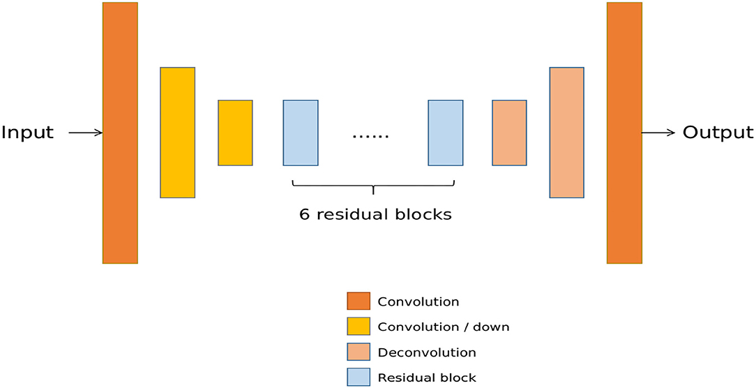
Figure A1. The network architecture of the generator Gs. It is a general ResNet (He et al., 2016) network for image-to-image translation.
The generator Gd from Jégou et al. (2017) is based on dense-block (DB), as Figure A2. Convolution denotes a 3 × 3 Convolution-BatchNorm-ReLU layer with 32 filters and stride 1. Transition down is a maxpool2d operation with the same number of filters and a 1 × 1 Convolution-BatchNorm-ReLU layer with the same number of filters and stride 1. Transition up denotes a 4 × 4 deconvolution layer with the same number of filters and stride 2. Dense block denotes four 3 × 3 BatchNorm-ReLU-Convolution layers with 12 filters and stride 1. The output channel number of the dense block is the concatenation from the output of four layers and the input. The encoder and the decoder concatenate with skip connection.
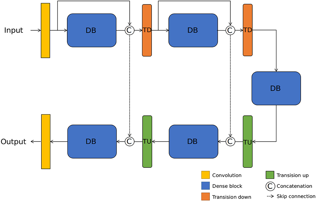
Figure A2. The network architecture of the generator Gd. Following the work of UW-Net (Gupta and Mitra, 2019), we choose DenseNet (Jégou et al., 2017) as the generator Gd.
Discriminator Architectures
For discriminator networks, we use 70 × 70 PatchGANs (Isola et al., 2017; Zhu et al., 2017a). Similarly, we do not use InstanceNorm or BatchNorm in any layer and use leaky ReLUs with a slope of 0.2. The discriminator Ds has two outputs from the discrimination branch and the classification branch. Differently, the discriminator Dd only has one discrimination output.
Keywords: underwater vision, underwater depth map estimation, underwater image translation, generative adversarial network, image-to-image translation
Citation: Zhao Q, Zheng Z, Zeng H, Yu Z, Zheng H and Zheng B (2021) The Synthesis of Unpaired Underwater Images for Monocular Underwater Depth Prediction. Front. Mar. Sci. 8:690962. doi: 10.3389/fmars.2021.690962
Received: 05 April 2021; Accepted: 23 August 2021;
Published: 17 September 2021.
Edited by:
Jun Li, University of Technology Sydney, AustraliaReviewed by:
Boguslaw Cyganek, AGH University of Science and Technology, PolandAncheng Lin, University of Technology Sydney, Australia
Copyright © 2021 Zhao, Zheng, Zeng, Yu, Zheng and Zheng. This is an open-access article distributed under the terms of the Creative Commons Attribution License (CC BY). The use, distribution or reproduction in other forums is permitted, provided the original author(s) and the copyright owner(s) are credited and that the original publication in this journal is cited, in accordance with accepted academic practice. No use, distribution or reproduction is permitted which does not comply with these terms.
*Correspondence: Zhibin Yu, eXV6aGliaW5Ab3VjLmVkdS5jbg==
†These authors have contributed equally to this work