 Kathryn L. Gunn
 Alex Dickinson
 Nicky J. White1
 Colm-cille P. Caulfield
- 1Bullard Laboratories, Department of Earth Sciences, University of Cambridge, Cambridge, United Kingdom
- 2BP Institute, University of Cambridge, Cambridge, United Kingdom
- 3Department of Applied Mathematics and Theoretical Physics, University of Cambridge, Cambridge, United Kingdom
The southwest Atlantic gyre connects several distinct water masses, which means that this oceanic region is characterized by a complex frontal system and enhanced water mass modification. Despite its significance, the distribution and variability of vertical mixing rates have yet to be determined for this system. Specifically, potential conditioning of mixing rates by frontal structures, in this location and elsewhere, is poorly understood. Here, we analyze vertical seismic (i.e., acoustic) sections from a three-dimensional survey that straddles a major front along the northern portion of the Brazil-Falkland Confluence. Hydrographic analyses constrain the structure and properties of water masses. By spectrally analyzing seismic reflectivity, we calculate spatial and temporal distributions of the dissipation rate of turbulent kinetic energy, ε, of diapycnal mixing rate, K, and of vertical diffusive heat flux, FH. We show that estimates of ε, K, and FH are elevated compared to regional and global mean values. Notably, cross-sectional mean estimates vary little over a 6 week period whilst smaller scale thermohaline structures appear to have a spatially localized effect upon ε, K, and FH. In contrast, a mesoscale front modifies ε and K to a depth of 1 km, across a region of O(100) km. This front clearly enhances mixing rates, both adjacent to its surface outcrop and beneath the mixed layer, whilst also locally suppressing ε and K to a depth of 1 km. As a result, estimates of FH increase by a factor of two in the vicinity of the surface outcrop of the front. Our results yield estimates of ε, K and FH that can be attributed to identifiable thermohaline structures and they show that fronts can play a significant role in water mass modification to depths of 1 km.
1. Introduction
Gyres are a key component of the large-scale meridional overturning circulation since they provide exchange sites between warm and cold water masses. In the southwest Atlantic Ocean, the Brazil-Falkland Confluence connects subtropical with subantarctic water masses. This confluence is a region of significant water mass modification. Nevertheless, a paucity of sufficiently well-resolved observations has hampered efforts to understand the extent of water mass variability associated with vertical exchanges. Here, we address this knowledge gap by exploiting a seismic (i.e., acoustic) technology that enables full-depth vertical sections of thermohaline structure and vertical mixing rates to be recovered. These seismic sections are hundreds of kilometers long and complement hydrographic sections acquired by the Global Ocean Ship-based Hydrographic Investigations Program (GO-SHIP), albeit with a dramatically improved horizontal resolution of ~10 m.
The southward-flowing western boundary current of the South Atlantic subtropical gyre, known as the Brazil Current (BC), connects warm subtropical waters with cold subantarctic water masses of the northward flowing Falkland Current (FC; Figure 1A). Hydrographic transects, ship-based observations, and satellite measurements demonstrate that this region is a site of strong water mass modification (e.g., Bianchi et al., 2001; Saraceno et al., 2004). Jullion et al. (2010) showed that horizontal heat and salt exchanges account for up to one half of the total poleward heat flux across the Antarctic Circumpolar Current. These insights are necessarily based upon intermittently obtained hydrographic measurements that cannot easily constrain water mass modification which occurs as a result of vertical mixing. Thus, the distribution and variability of vertical mixing rates have yet to be diagnosed.
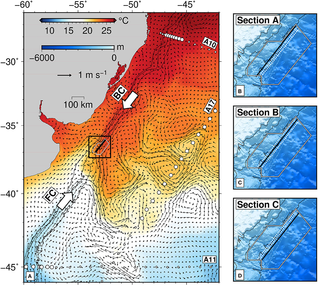
Figure 1. (A) Map of southwest Atlantic Ocean where red/blue colors represent warm/cold mean sea-surface temperatures for monthly composite centered on 16th February 2013 (taken from Multi-scale Ultra-high resolution (MUR) satellite sea-surface temperature measurements which have monthly and 1 km resolution). Thin black lines = 300/1,000/2,000 m bathymetric contours; field of black arrows = average sea surface geostrophic current velocities calculated for 5-day composite centered on 15 February 2013 from OSCAR satellite measurements (scale at top left-hand side); labeled arrows = Brazil Current (BC) and Falkland (i.e., Malvinas) Current (FC); black box = zoom region shown in panels (B–D); white polygon = location of 3D seismic reflection survey; thick black line within polygon = locus of three transects displayed in Figures 4–9; small white circles = loci of conductivity temperature depth (CTD) probes acquired as part of GO-SHIP transects A10 (December 1992), A17 (April 2019) and A11 (December 1992); large white circles = loci of CTDs used to compute average hydrographic profiles (Figure 2). (B–D) Zoomed portion shown in (A). Blue shading = water depth according to scale bar at top left-hand of (A); thin black lines = 300/1,000/2,000 m bathymetric contours; white polygon = location of 3D seismic reflection survey; solid black line inside polygon = seismic transect acquired on given date; dotted white lines = other transects.
Concentration of large-scale temperature gradients creates complex frontal systems, that tend to be important sites for water mass modification. Shallow (i.e., 0–500 m) observations obtained by towed instruments and floats demonstrate that the upper portions of fronts are often regions of enhanced vertical mixing (e.g., Nagai et al., 2009, 2015; D'Asaro et al., 2011; Johnston et al., 2011; Peng et al., 2020). These locations can contribute significantly to the vertical re-distribution of heat and salt, thus impacting thermohaline circulation (Liang et al., 2015; Frazão and Waniek, 2021). A paucity of observations in the southwest Atlantic Ocean has left a gap in our understanding of the magnitude and variability of vertical heat fluxes in the Brazil-Falkland Confluence. Even less is known about the role that fronts play in moderating dissipation rates at depths greater than ~500 m.
Here, we address these knowledge gaps with the aid of seismic reflection profiling. This technology exploits low (i.e., 5–100 Hz) frequency sources and multiple towed cables with dense arrays of hydrophone receivers (Holbrook et al., 2003; Ruddick et al., 2009). Acoustic waves are transmitted through, and reflected from, temperature fluctuations on length scales that vary from tens of meters to tens of kilometers. The resultant seismic sections can be used to delineate and map oceanic structure and water masses with contrasting thermohaline properties over a hitherto unsurpassed range of scales (e.g., Sallarès et al., 2009; Sheen et al., 2012; Gunn et al., 2018). Resultant images can be inverted and spectrally analyzed to obtain simultaneous distributions of temperature and vertical mixing rates, respectively, that span the full depth of the water column (e.g., Dickinson et al., 2017; Gunn et al., 2020). This emerging field of research is generally referred to as Seismic Oceanography.
We analyze thermohaline structures and mixing properties across a portion of the northern Brazil-Falkland Confluence. First, we describe three seismic sections that straddle this confluence, spanning a period of 6 weeks between 1st February 2013 and 15th March 2013. Each of these sections is ~140 km in length. They were acquired sequentially and any one section is laterally offset by several kilometers. Our study builds upon a previously published contribution which describes the structure and hydrographic properties of a deeply penetrating front and of a transient mesoscale eddy that both advect across the seismic survey (Gunn et al., 2020). Secondly, we spectrally analyze these seismic sections in order to calculate spatial distributions of diapycnal mixing rates, which can then be combined with seismically determined temperature profiles to estimate vertical diffusive heat fluxes. Finally, we compare recovered distributions of mixing and heat flux with observed oceanographic processes and we discuss how these distributions may evolve as a function of time.
2. Observational Constraints
2.1. Seismic Reflection Survey
We present time-lapse imagery extracted from a three-dimensional (3D) seismic reflection survey that straddles a small northern portion of the Brazil-Falkland confluence of the southwest Atlantic Ocean (Figure 1A). This seismic survey was acquired between November 2012 and April 2013 by Polarcus Limited OSE. During acquisition, a pair of alternately firing airgun arrays, each of which has 36 guns with a combined volume of 70 L (4240 in3), were deployed off the stern of the vessel at a depth of ~5 m. Ten streamers (i.e., acoustically sensitive cables), each of which is 6 km in length, were towed behind the vessel (for further details see Gunn et al., 2020). The vessel steamed with an average azimuth of 41° in what is known as the racetrack mode of acquisition at an average speed of 2.5 m s−1 (Yilmaz, 2001). Each individual pass of the vessel acquired a single 3D swath of seismic data that is ~120–150 km long and ~600 m wide. The seismic sections presented here are extracted from the center of each swath which were acquired between 1st February 2013 and 15th March 2013 (Figures 1B–D and Table 1).
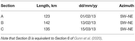
Table 1. Seismic acquisition information (Figure 1).
2.2. Hydrographic and Satellite Observations
Independent hydrographic and satellite observations are used to calibrate this seismic reflection survey. Coincident and dense hydrographic measurements are unavailable. Instead, we exploit conductivity-temperature-depth (CTD) profiles from three nearby GO-SHIP transects (A10, A11, and A17). These transects approximately bound the Brazil-Falkland Confluence at its northern, southern and eastern boundaries, respectively (Jullion et al., 2010). Given the planform of the Brazil and Falkland Currents, these transects are representative of BC (i.e., subtropical), FC (i.e., subantarctic), and mixed water masses, respectively (Figure 1). A subset of CTD casts from each GO-SHIP transect are used to generate average profiles of temperature and salinity (Figure 2). Along transects A10 and A11, these CTD casts are positioned away from the continental shelf and extend offshore by the approximate width of the Brazil and Falkland Currents, respectively (Figure 1A). For transect A17, a monthly composite of sea surface currents and float trajectories are used to gauge the latitudinal range of enhanced eddy kinetic energy associated with the confluence between 34 and 42° S (Iglesias, 2019). We conclude that these average profiles are representative of water masses entering and exiting the confluence at the location of the seismic survey.
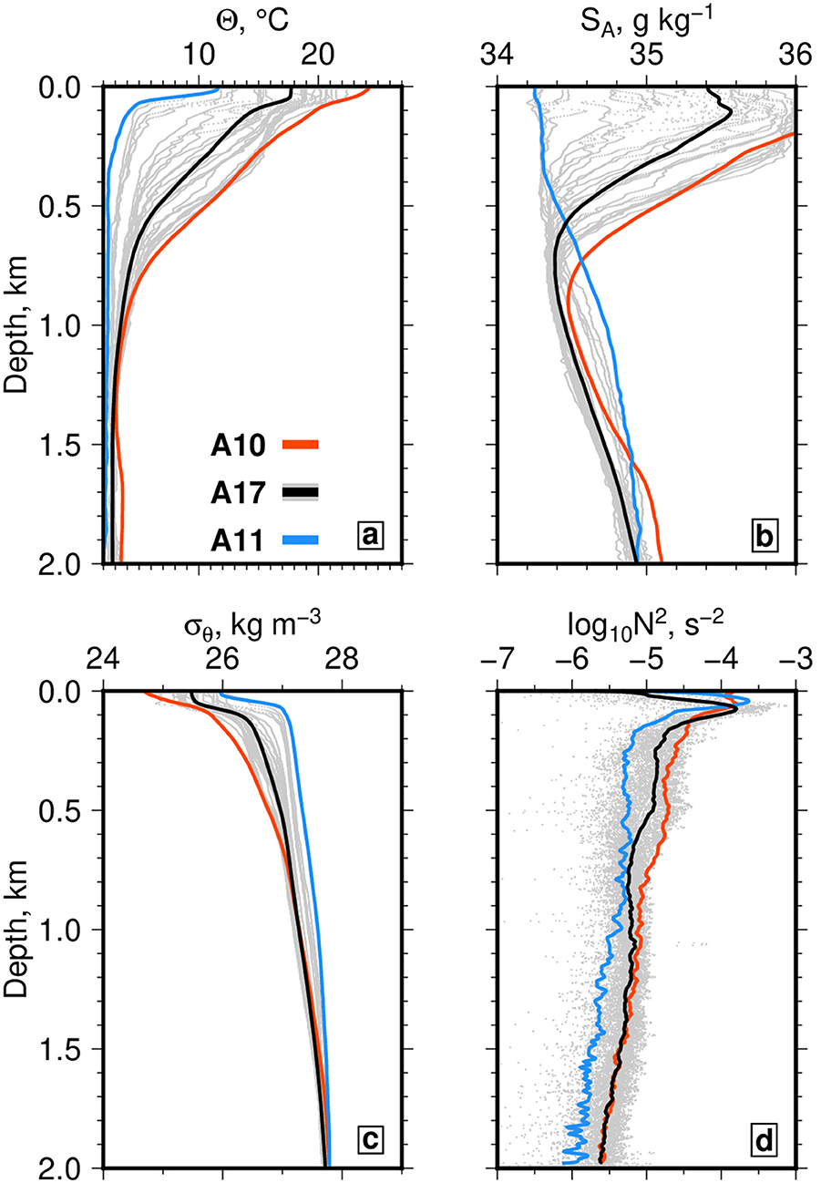
Figure 2. Hydrographic profiles calculated from CTD casts acquired along GO-SHIP sections A10, A11, and A17 that are representative of subtropical, subantarctic and intermediate water masses, respectively (see Figure 1A for location). (A) Conservative temperature, Θ, plotted as function of depth. (B) Absolute salinity, SA, plotted as function of depth. (C) Potential density anomaly, σθ, plotted as function of depth. (D) Buoyancy (Brunt-Väisälä) frequency squared, N2, plotted on logarithmic scale as function of depth. In each panel, gray lines = individual profiles of A17 casts; red line = average profile calculated from 8 CTD casts along A10; blue line = average profile calculated from 8 CTD casts along A11; black line = average profile calculated from 14 CTD casts acquired along A17 (see enlarged white circles in Figure 1A). All profiles smoothed using 100 m low-pass Butterworth filter.
Maps of sea surface temperature for the southwest Atlantic Ocean highlight the confluence of warm and cold water masses (Figure 3). Confluent flow of warm BC and cold FC concentrates large-scale temperature gradients that are clearly visible in satellite imagery, generating a frontal system that is marked by several discrete fronts which occur between 36 and 39° S (Gordon, 1989; Peterson and Stramma, 1991). Temperature maps also show the variability in the location and properties of this confluence as a function of time. They are consistent with other satellite observations, which confirm the presence of this oscillation of the Brazil–Falkland Confluence at this time of year (Garzoli and Garraffo, 1989; Saraceno et al., 2004; Combes and Matano, 2014). After converging, sea surface current and float trajectory measurements show that these subtropical and subantarctic water masses turn eastward, spreading out into the center of the Atlantic Ocean (Figure 1; Iglesias, 2019).
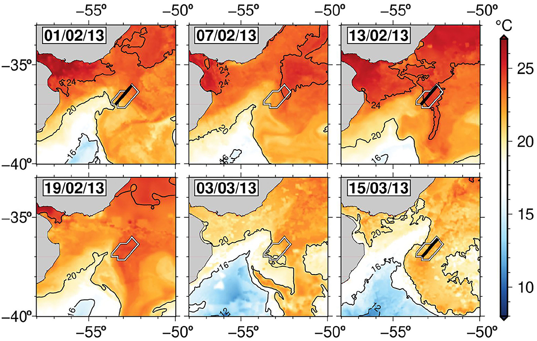
Figure 3. Selected maps of sea-surface temperature for southwest Atlantic Ocean showing temporal variability of Brazil-Falkland Confluence. Red/blue colors = warm/cold sea surface temperatures from 1st February 2013 to 15th April 2013 (date shown at top left-hand side). Satellite sea-surface temperature observations from L4 gridded products of GHRSST database that have daily and 1 km resolutions. White polygon = location of 3D seismic survey; thick black line = loci of seismic sections for 01/02/13, 13/02/13, and 15/03/13; thin black lines = sea surface temperature contoured at 4° C intervals.
3. Methods
3.1. Signal Processing of Seismic Imagery
In the context of Seismic Oceanography, an important goal is to combine individual seismic records to order to generate an image which represents a full-depth vertical section through the water column (Figure 4A). To construct these sections, we adopt standard signal processing techniques that have previously been applied to this survey and that are described in more detail by Gunn et al. (2020). Significant processing steps include application of a 20–90 Hz band-pass filter with a roll-off of 24 dB per octave, muting of the bright and irregular sea-bed reflection, removal of high amplitude acoustic energy that travels horizontally along the length of each streamer (i.e., the direct arrival), velocity picking, and stacking (i.e., combining multiple seismic records). The data used to construct a single stacked section take several hours to acquire since the vessel steams at ~2.5 m s−1. It is important to emphasize that during the stacking process, many repeated shot-receiver pairs that image an identical portion of the sub-surface are summed together. The vertical resolution of a seismic section is given by v/(4f) where v and f are the speed of sound through water and the dominant frequency of the acoustic source, respectively. In this region, v = 1,510 ± 30 m s−1 and the peak value of f = 35± 5 Hz, which yields a nominal vertical resolution of 10–20 m (Gunn et al., 2020). In contrast to GO-SHIP transects, vertical and horizontal resolution are equal.
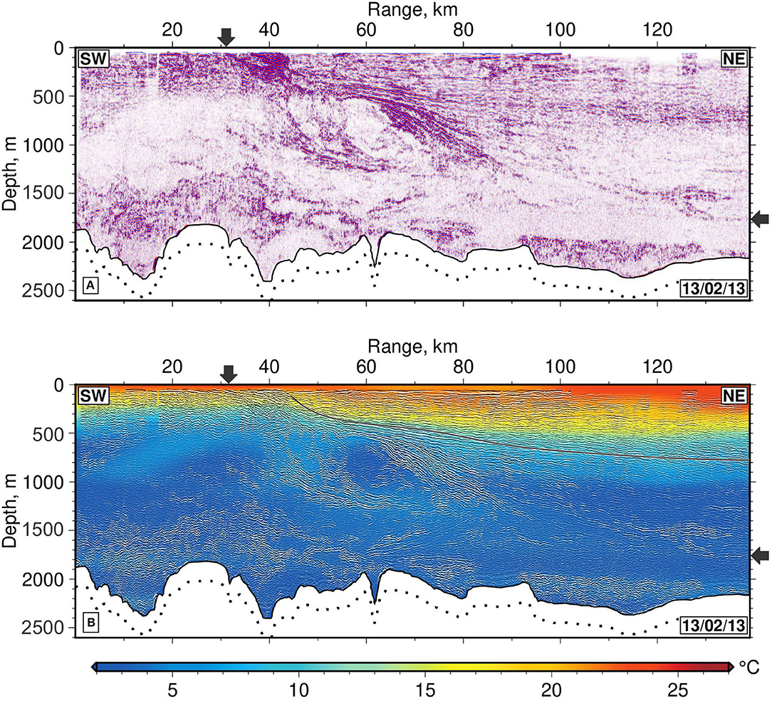
Figure 4. (A) Seismic reflection section B that crosses oceanic front (see also Figure 1C and panel dated 13/02/13 of Figure 3). Red/blue stripes represent positive/negative polarity reflections generated by temperature changes as small as ~ 0.01°C within water column; irregular solid/dotted lines = seabed; black arrows = maximal extent of front at sea surface and at depth. (B) Corresponding conservative temperature field calculated using iterative inversion procedure (Gunn et al., 2018, 2020). Warm/cool colors = temperatures according to scale bar; solid black line = smoothed potential density anomaly contour of 26.8 kg m−3 which highlights shallowest sub-surface expression of front (see Figures 3, 8E,F of Gunn et al., 2020 for more detailed treatment).
The observed reflectivity is generated by changes in acoustic impedance (i.e., the product of sound speed and density). Within the water column, acoustic impedance is predominantly controlled by sound speed variation, which depends upon temperature gradient and, to a much lesser extent, upon salinity gradient (Sallarès et al., 2009). When confluent flow of warm subtropical and cold subantarctic water masses concentrates large-scale temperature gradients across a large region, this confluence is characterized by strong impedance contrasts which gives rise to bright reflectivity (Figure 4A). In summary, each seismic section represents a near-instantaneous, full-depth vertical slice through the oceanic volume that is essentially a well-resolved map of vertical temperature gradient.
3.2. Seismically Determined Properties
The temperature distribution along each seismic section is calculated using an adapted iterative method (Papenberg et al., 2010; Gunn et al., 2018, 2020). Acoustic inverse schemes that rely upon densely sampled hydrographic measurements are less easy to exploit since coincident observations of temperature and salinity are unavailable (Azevedo et al., 2021). Instead, we use a pragmatic approach that side-steps this limitation and takes advantage of the dominant dependency of acoustic sound speed upon temperature. First, we construct the long-wavelength sound speed field for each section by analyzing pre-stack seismic records (Figures 6, 7 of Gunn et al., 2020). Secondly, each sound speed field is iteratively converted into an equivalent distribution of temperature using the equation of state for seawater.
Due to a paucity of coeval hydrographic measurements, we reasonably assume that density varies as a function of depth and that salinity is a function of both temperature and depth, which can be estimated at 10 m depth intervals. The temperature-salinity relationship is calculated from the regional CTD casts shown in Figures 1A, 2 and it is in accordance with regional hydrographic measurements (Gunn et al., 2020). Given these assumptions, seismic sections can be converted into temperature (Figure 4B). Seismically derived temperature and salinity estimates enable contemporaneous fields of vertical temperature gradient and of density to be estimated which can then be used to calculated vertical diffusive heat fluxes (Equation 3). Note that recovery of temperature fields from seismic images is contingent upon the distribution of horizontally continuous reflections. As a consequence, there is greater uncertainty in the details of any recovered field beneath 1,000 m and above ~150 m where reflections can be difficult to trace see Figure 6 of (Gunn et al., 2020). Nevertheless, this method is a useful way to calculate contemporaneous temperature fields, especially because it enables the vertical temperature gradient to be recovered. A conservative depth-averaged uncertainty of seismically determined temperature estimates is ≤ ±1° C (Gunn et al., 2020).
3.3. Dissipation and Diapycnal Mixing Rates
Oceanic circulation is maintained by the cascade of energy from large-scale flows down to the smallest length scales of turbulent mechanical mixing (Munk, 1966). On horizontal length scales of 0.1–10 km, this cascade can be interrogated by tracking and spectrally analyzing reflections from stacked seismic sections (e.g., Sheen et al., 2009; Holbrook et al., 2013; Dickinson et al., 2017). Small vertical displacements along quasi-horizontal reflections record perturbations of the background stratification caused by a combination of internal waves and turbulence. Variations in the size of these vertical displacements as a function of horizontal wavelength are obtained by calculating the power spectrum of vertical displacements as a function of horizontal wavenumber kx. This approach enables the internal wave and turbulent subranges to be identified and modeled to obtain the dissipation rate of turbulent kinetic energy, ε, and thence diapycnal diffusivity, K. Sheen et al. (2009) and Holbrook et al. (2013) demonstrated that seismic reflections generally track isopycnal surfaces and they showed that the turbulent subrange can be reliably isolated with careful signal processing. The methodology is divided into three stages (Figure 5).
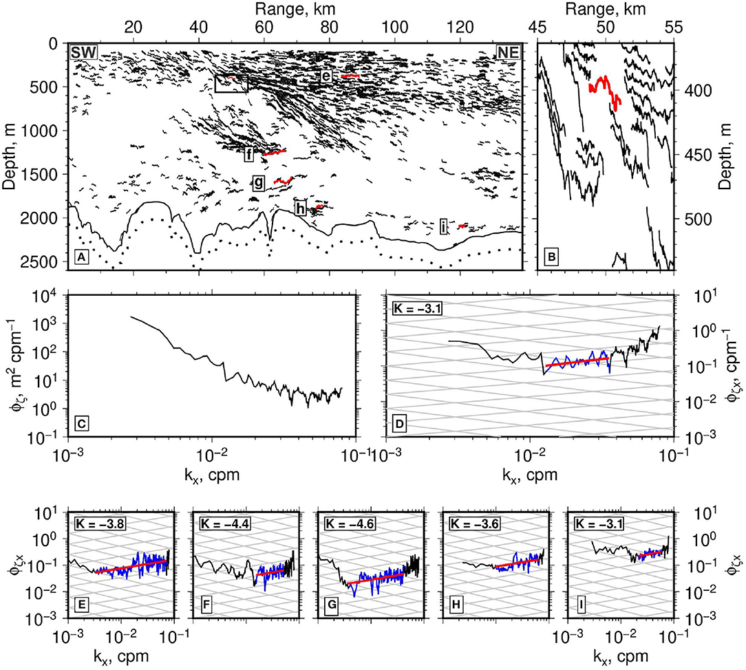
Figure 5. (A) Auto-tracked version of section B. Black box = zoomed portion shown in (B,C) where red line = auto-tracked reflection analyzed in (C,D); labeled red lines = auto-tracked reflections that are spectrally analyzed in (E–I). (B) Zoomed portion of (A) with auto-tracked reflection that is spectrally analyzed in (C,D). (C) Power of vertical displacement, Φξ, plotted as function of horizontal wavenumber, kx, which has units of cycles per meter (cpm). Spectrum calculated using multi-taper Fourier transform of linearly detrended tracked reflection highlighted in (B). Internal wave, turbulent, and noise subranges characterized by spectral slopes of −2, −5/3 and 0, respectively. (D) Φξx (i.e., Φξ × ) plotted as function of kx. On this slope spectrum, black/blue/black lines = internal wave/turbulent/noise subranges characterized by spectral slopes of −1/2, +1/3 and +2, respectively; red line = best-fitting model of turbulent subrange; label in top right = calculated value of log10 K; gray reticule = slopes of internal wave and turbulent subranges with spectral gradients of −1/2 and +1/3, respectively. (E–I) Slope spectra for other auto-tracked reflections shown in (A). Symbols and labels as for (D).
3.3.1. Tracking Reflective Events
Each trace of seismic amplitude is converted into the cosine of the instantaneous phase angle. Application of this seismic attribute helps to emphasize the continuity of reflections in a way that does not influence resolution of the seismic image (Holbrook et al., 2013). Reflective events are tracked by contouring with a constant value of the instantaneous phase (Figure 5A). The choice of contour value does not affect the geometry of tracked reflections but it can influence the number of tracked reflections (Dickinson et al., 2017). Reflections with lengths that are greater than 1 km are chosen since they yield the best-resolved spectra. At this stage, the midpoints along each contoured event are calculated and taken to represent isopycnal surfaces, thus providing information about horizontal wavenumber, kx. These midpoints are used to estimate vertical displacements of the isopycnal surfaces (Figure 5B).
3.3.2. Spectral Analysis of Tracked Reflections
Power of vertical displacement, Φξ, as a function of kx is calculated from each linearly detrended tracked reflection using a multi-taper Fourier Transform, F(kx), where (Thomson, 1982). Φξ is a measure of the power distribution of the decomposed signal as a function of kx (Figure 5C). Horizontal wavenumber power spectra are converted into power spectra of the horizontal gradient of vertical displacement, Φξx, by multiplying Φξ by (Klymak and Moum, 2007a,b). Φξx(kx) is usually referred to as the slope spectrum.
In the oceanic realm, slope spectra calculated from seismic images, as well as from autonomous gliders, reveal two distinctive regimes with the characteristic spectral slopes of the internal wave and turbulent components of the oceanic energy spectrum (Klymak and Moum, 2007a,b; Sheen et al., 2009). The internal wave regime is visible at low wavenumbers of m−1, corresponding to horizontal length scales of >100–1,000 m (Figure 5D). At high wavenumbers of m−1, internal waves break and there is a clear transition to a regime with a characteristic turbulent spectral slope. The spectral slope of this regime matches the Kolmogorov exponent of −5/3 which, when multiplied by to create horizontal gradient (i.e., slope) spectra, becomes +1/3 (Spalding, 1991). Significantly, this slope is still observed at horizontal scales that exceed the Ozmidov length scale, which means that a slope of −5/3 should not be thought of as purely isotropic turbulence. At these longer scales, this slope probably represents layered anisotropic stratified turbulence (LAST; Riley and Lindborg, 2008; Falder et al., 2016). White noise has a gradient of +2 and is clearly visible at the highest wavenumbers (e.g., m−1). Given this ability to seismically identify spectral slopes, it is possible to model the observed turbulent subrange and to estimate both the dissipation rate of turbulent kinetic energy, ε, and the diapycnal diffusivity, K.
3.3.3. Dissipation and Diffusivity Calculations
It is straightforward to identify internal wave, turbulent, and white (i.e., ambient) noise subranges by examining Φζx(kx) spectra (Figures 5E–I). Here, we focus on analyzing observed turbulent subranges following the approach described by Sheen et al. (2009) and later refined by Dickinson et al. (2017). For a given spectrum, the gradient of the turbulent subrange, the co-ordinates of the intersection between the internal wave and turbulent subranges, and width of the turbulent subrange determine the value of Φζx(kx). A misfit function that measures the difference between observed and calculated values of Φζx(kx) is minimized by adjusting the values of gradient, co-ordinates of intersection, and width for each spectrum (see Appendix D3 of Dickinson et al., 2020). In this way, Φζx(kx) is calculated for each spectrum and used to estimate the turbulent dissipation rate, ε, using a simplified version of the Batchelor et al. (1959) model where
CT = 0.4 is the Obukhov-Corrsin constant, Γ = 0.2 is the turbulent flux coefficient, and N is the Brunt-Väisälä (i.e., buoyancy) frequency which is obtained from regional hydrographic measurements [i.e., Figure 2 D black line; (Osborn, 1980; Mashayek et al., 2017)]. Since the observed turbulent subrange extends to wavenumbers that are smaller than the Ozmidov scale, our use of this inertial-convective parametrization implicitly assumes that there is continuity between the LAST and inertial-convective regimes (Riley and Lindborg, 2008). Finally, diapycnal diffusivity, K, is obtained using the Osborn (1980) relationship where
Spatial variations of ε and K for Section B are presented in Figure 6.
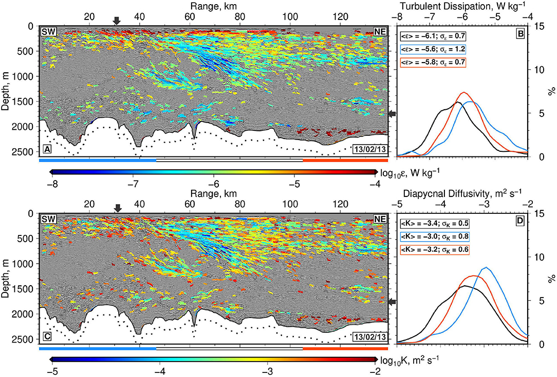
Figure 6. (A) Spatial variation of turbulent dissipation rate, log10 ε, for section B where warm/cool colors indicate higher/lower values according to scale bar along base of panel; black arrows = maximal extent of front at sea surface and at depth. (B) Histogram showing spatially averaged distribution of dissipation, <ε>. Envelopes calculated using bin widths of 0.1 and Gaussian filter lengths of 1 for spatial ranges of 0–40 (blue), 40–90 (black line and white bar), and 90–140 km (red). (C,D) Same for spatial variation of diapycnal mixing, log10 K and its average value, <K>.
3.4. Diffusive Heat Flux
The diapycnal diffusive heat flux, FH, is calculated in accordance with standard molecular (Fickian) diffusion where
ρ∘ is potential density, Cp is the isobaric heat capacity of seawater, and dΘ/dz is the vertical gradient of conservative temperature. Here, we calculate the spatial and temporal variability of FH using temperature and density fields obtained from calibrated seismic reflection sections together with the spatial and temporal variation of K (e.g., Figures 4B, 6C). So, the four parameters on the right-hand side of this equation vary as a function of time and space. Since the nominal vertical resolution is O(10) m, values of dT/dz, ρ∘, and Cp are measured at intervals of 10 m. The units of FH are W m−2 where positive heat flux is downward. Note that our estimates of FH do not take advective contributions into account since well-resolved velocity measurements are unavailable.
3.5. Uncertainty Estimates
Following Dickinson et al. (2020), the maximum likely uncertainty for log10 K is ±0.4 logarithmic units. This value is gauged in the following way. First, uncertainty in N is given by its standard deviation which is ±0.3 cph. This uncertainty is combined in quadrature with the uncertainty of the fitted intercept (i.e., 0.02–0.1) to yield an estimated mean uncertainty for log10 K of ±0.15 logarithmic units. Secondly, we acknowledge that assuming constant values of CT and Γ is a significant simplification (Mashayek et al., 2017). This assumption can be tested by considering their upper and lower bounds, which yields a maximum uncertainty of ±0.25 logarithmic units (Dickinson et al., 2020). Notwithstanding uncertainties associated with absolute values of mixing rate, we are confident that these relative variations are robust.
Given that the conservative upper bound of uncertainty for log10 K is ±0.4 logarithmic units, the propagated uncertainty for FH can be estimated by combining uncertainties for log10 K and dΘ/dz. The uncertainty for Θ is conservatively estimated as ±1° C (Gunn et al., 2020). After taking the vertical gradient over 10 m, we obtain an uncertainty of ±0.1 K m−1 for dT/dz. Uncertainties for ρ∘ and Cp are ±0.1 kg m−3 and ±0.8 J kg−1 K−1, respectively. Thus, the propagated uncertainty for our estimates of FH is ±3 W m−2.
4. Results
4.1. Water Mass Structure
On Section B, which was acquired on 13th February 2013, the most obvious feature is a band of gently dipping reflectivity that crops out at the sea surface over a range of 30–40 km (Figure 4A). This band represents a deeply penetrating front. Over much of its length, a bright and continuous reflection that dips northward is visible that can be traced down to a depth of 1.8 km. This front separates a wedge of smooth and horizontally continuous reflections to the north from more discontinuous, and even swirling, reflectivity to the south. A prominent tilted lens with a complex pattern of internal reflectivity centered at a range of 60 km sits against the front. Within 400 m of the sea surface, the front splits into a several strands that encase lens-shaped and acoustically transparent features that are interpreted as intra-thermoclinic eddies (Gunn et al., 2020). On both sides of the front, the thermocline is generally visible as a band of reflectivity that extends to a depth of 1,000 m which is consistent with hydrographic measurements (Figure 2). The calculated temperature field shows that the northern end of Section B is characterized by a wedge of warm subtropical water, the Brazil Current, that abuts the front (Figure 4B). South of the front, cooler temperatures are consistent with the presence of an intermediate water mass generated by mixing of subtropical and subantarctic waters.
On Section A, which was acquired on 1st February 2013, a thick band of approximately flat reflectivity that extents to a depth of 1,000 m defines the thermocline (Figure 7A). The vertical extent of the thermocline is corroborated by the horizontally averaged temperature distribution extracted from the seismic image (Figure 7B). From the sea surface down to a depth of 1,000 m, temperature values decreases from 25 to 5°C, which is comparable to the observed temperature distribution of subtropical water masses along GO-SHIP transect A10 (Figure 2A). Temperatures of ~5°C are diagnostic of AAIW, CDW, and NADW at these depths (Piola and Matano, 2017). At the northeastern end of Section A, the thermocline terminates in a set of bright reflections which are abruptly cut off at a range of 100 km by weaker dipping reflections. We interpret this pattern of localized reflectivity as the upper portion of a partially imaged front. This intepretation is consistent with coeval surface temperature measurements (Figure 3). Beneath a depth of 1,000 m, water masses are characterized by complex swirling patterns of reflectivity that form a mixture of lenses and filaments that deform as a function of time (Gunn et al., 2020). A vortex-like structure, reminiscent of that observed between subtropical and subantarctic water masses at the Subantarctic Front by Sheen et al. (2011), occurs at a depth of 1,000 m centered at a range of 105 km. These complex reflection patterns imply that imaged water masses are deforming and/or undergoing lateral displacement. Considerable mixing is probably also occurring.
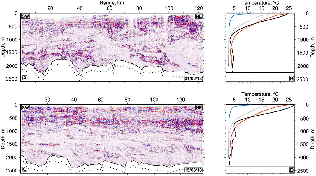
Figure 7. (A) Section A of seismic reflection survey. (B) Conservative temperature as function of depth. Black line = horizontally averaged temperature profile calculated for Section A using iterative inversion procedure; dashed line = portions of same profile where calculation is uncertain due to lack of continuous reflections at depths ≳1,000 m; red/blue/gray lines = average temperature profile obtained from GO-SHIP hydrographic sections A10/A11/A17, which represent subantarctic/subtropical/mixed water masses, respectively (see Figure 1A). (C) Section C of seismic reflection survey. (D) Same as (B) for Section C.
On Section C, which was acquired on 15th March 2013, the front is no longer visible (Figure 7C). Instead, layered and continuous reflections form a 1,000 m thick band that extends across the entire section. Beneath 1,000 m, sparser reflectivity delineates elongated filaments of O(10) km lengthscales. As in the case of Sections A and B, the average temperature distribution indicates that this section is representative of subtropical water masses (see Figure 7D). Apart from methodological uncertainties, seismically-derived property distributions are limited by the observed density of continuous horizontal reflections. Due to the limitations of seismic acquisition, reflections are often not clearly imaged at depths shallower than ~150 m. On the seismic sections presented here, there is also limited reflectivity at depths that exceed 1,000 m (Figures 7B,D). At these depths, horizontally averaged temperature profiles are inevitably less well constrained and tend to be discrepant with respect to hydrographic observations. Nonetheless, it is important to note that the vertical temperature gradient is faithfully recovered.
Given the depth and temperature of the thermocline together with the location of the seismic survey with respect to the confluence during February 2013, these seismic sections evidently cross the northern portion of the confluence since it is characterized by subtropical water masses of the Brazil Current (Figure 1A). The thermocline has a vertical extent of 1,000 m, which is consistent with steep temperature gradients observed within these subtropical water masses (Figures 7B,D; Piola and Matano, 2017). These observations are consistent with sea surface temperatures, which demonstrate that the seismic survey straddles the warmer portion of the confluence during February and March 2013 (Figure 3). Over a 6 week period, the depth of the thermocline remains consistent and its continuity is only disrupted adjacent to the dipping front, most likely the Brazil Current Front whose appearance and disappearance is caused by the observed oscillation of the confluence at this time of year (Olson et al., 1988; Saraceno et al., 2004; Severov et al., 2012; Gunn et al., 2020). The patterns of reflectivity also reveal other transient oceanic processes, including deformation of filaments and lenses, which have previously been interpreted as manifestations of stirring and cross-frontal mixing (Jullion et al., 2010; Gunn et al., 2020). This complex vertical and horizontal thermohaline structure has previously been observed on lengthscales of tens of kilometers using CTD probes (Reid et al., 1977; Gordon, 1989; Bianchi et al., 2001).
4.2. Vertical Mixing Rates
Section B demonstrates that dissipation and mixing rates are conditioned by the presence of a front (Figure 6). On the southern, denser side of the front, mixing rates are highest (e.g., 10−3–10−2 m2 s−1), especially at ranges of 20–40 km where the front crops out at the sea surface. North of a range of 40 km, the front deepens and its different reflective strands are characterized by suppressed mixing rates of ~10−4 m2 s−1 (Figure 6C). Similarly low mixing rates are found at the base of the prominent tilted lens. Beyond a range of 90 km, mixing rates increase up to values of ~10−3–10−2 m2 s−1. These qualitative observations are supported by full-depth weighted mean values of log10 ε (i.e., –6.1, –5.6, –5.8) and log10 K (–3.0, –3.4, –3.2) for ranges of 0–40, 40–90, and 90–140 km, respectively (Figure 6D). These section-averaged values reveal the overall effect that the front has upon vertical mixing rates— mixing is enhanced at its surface outcrop but it is locally suppressed along its dipping interface down to a depth of about 1 km.
Two weeks earlier (i.e., 1st February 2013), dissipation and mixing estimates for Section A range over three orders of magnitude (Figures 8A,C). Recovered estimates are much more spatially patchy which is consistent with the observed patterns of reflectivity. The highest mixing rates occur beneath the mixed layer (e.g., ~200 m) and in association with small-scale structures at ranges of 30–40 km and depths of 1,000–1,400 m. Lowest mixing estimates occur adjacent to the front at the northeastern portion of Section A between 100 and 120 km. A weighted histogram of recovered mixing estimates indicates that the mean, <K>, and standard deviation, σK, of log10 K are −3.2 and 0.5, respectively (Figure 8D). One month later, the thermocline is much more continuous and the deeply penetrating front is no longer visible (Figures 8E,G). Mixing rates are lowest in the thermocline and greatest at the base of the mixed layer with sporadically higher mixing throughout the deeper portions of the water column. <K> is 10−3.5 m2 s−1 (i.e., ~3×10⁻⁴ m2 s−1), which is consistent with mean values calculated for the two other sections.
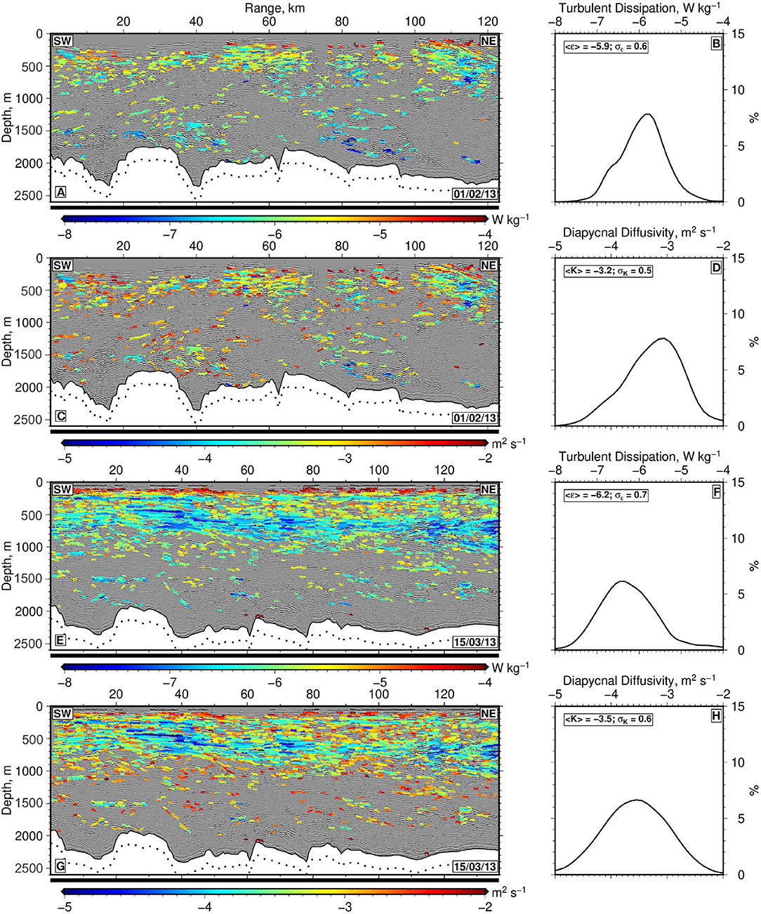
Figure 8. (A) Section A of seismic reflection survey overlain with spatial distribution of turbulent dissipation rate, log10 ε, calculated using spectral analysis of tracked reflectivity. Colored wiggly lines = 1,841 auto-tracked reflections where color indicates value of log10 ε according to scale bar at base of (E). (B) Histogram showing spatially averaged distribution of log10 ε for (A) calculated using bin width of 0.1 and Gaussian filter length of 1. Numbers = weighted mean, <ε>, and standard deviation, σε, of values from Section A. (C) Same overlain with spatial distribution of diapycnal diffusivity, log10 K. Colored wiggly lines = individual auto-tracked reflections where color indicates value of log10 K according to scale bar at base of (E). Note that global mean log10 K is –5 (e.g., Waterhouse et al., 2014) and that uncertainty of calculated log10 K is 0.4. (D) Histogram showing spatially averaged distribution of K. (E–H) Same for Section C with 2,310 tracked reflections.
Mixing rates calculated for other seismic sections that also image the deeply penetrating front have similar spatial patterns of diapycnal diffusivity. Given our conservative estimate of uncertainty of ±0.4 for log10 K, these observed patterns of diapycnal diffusivity— enhanced K the surface outcrop of the front and suppressed values of K along its dipping interface— are robust. We conclude that this front conditions mixing rates on lengthscales of O(10–100) km.
4.3. Diffusive Heat Flux
Seismically-derived heat fluxes, FH, range from –3 to 10 W m−2 (Figure 9). For all three seismic sections, the highest values of FH occur along the base of the mixed layer. FH decreases with depth along each seismic section (Figures 9A,C,E). Horizontally averaged profiles show that there is a marked decrease in the value of FH from 1–8 W m−2 at the sea surface to 0 W m−2 at 1,000 m depth (Figures 9B,D,E). Profiles of FH calculated using the mean Θ(z) distribution taken from transect A17 show the same trend within uncertainty (Figures 9B,D,F dashed lines). This behavior is expected since FH describes Fickian diffusion, by which mixing rate acts upon vertical temperature gradient. Since dΘ/dz decreases with depth, the effect of mixing becomes increasingly limited. The vertical variation of FH for sections A and C is broadly similar. Therefore, at mesoscale length scales in the absence of a front, FH does not appear to significantly change over the 6 week period.
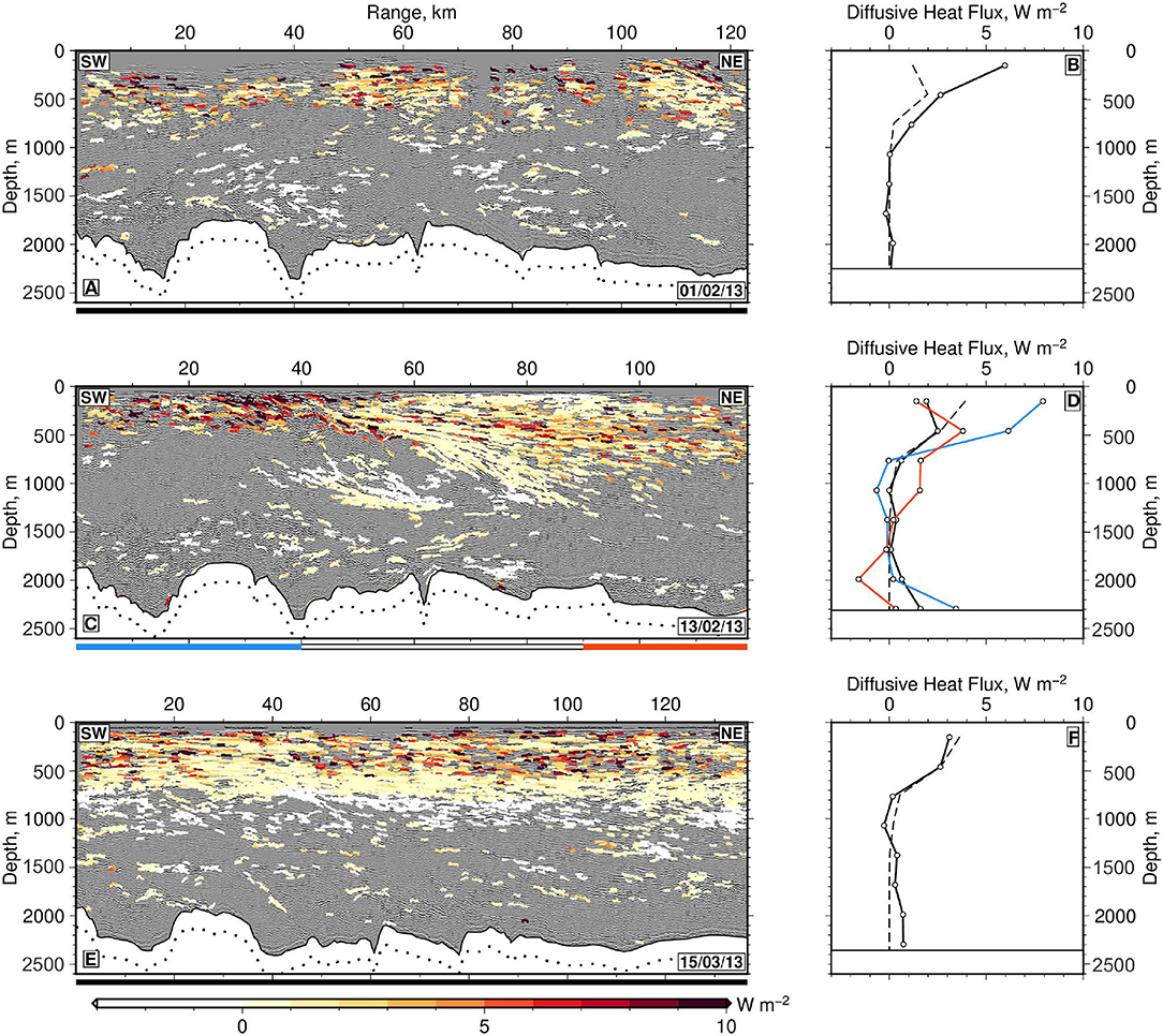
Figure 9. (A) Section A of seismic reflection survey overlain with spatial distribution of vertical diffusive heat flux, FH, calculated using seismically determined mixing estimates and temperature distribution. Colored wiggly lines = 1,017 auto-tracked reflections where color indicates value of FH according to scale bar at base of (E). Positive values indicate downward-directed heat flux and uncertainty in FH is 3 W m−2. Black bar along base of image = range used to calculate horizontal mean of FH reported in (B). (B) Horizontal mean of FH in 300 m depth bins. White circles and solid black line = binned mean values of FH calculated using seismically, determined values of Θ(z); dashed black line = binned mean values of FH calculated using CTD-measured values of Θ(z) (see Figure 2A). (C,D) Same for Section B with 1,841 tracked reflections. Blue/white/red bar along base of image = three ranges used to calculate horizontally averaged profiles of FH. (E,F) Same for Section C with 2,310 tracked reflections.
On the other hand, we also observe conditioning of FH by the front itself (Figures 9C,D). Close to the surface outcrop of the front, heat fluxes reach their greatest values (Figure 9D). Enhancement of these heat fluxes exceeds the uncertainty of ±3 W m−2 and it is directly associated with the vigorous mixing observed here (Figure 6C). Along the dipping boundary of the front, FH is also elevated. Here, elevated values are a result of the significant vertical temperature gradient caused by the presence of a wedge of warm water that is banked up against the front where it overlies cooler water (Figure 4B). We conclude that this major front conditions vertical diffusive heat flux on length scales of O(10–100) km.
5. Discussion
A suite of seismic reflectivity sections is employed to shed light on the internal structure of a small portion of the northern Brazil-Falkland Confluence— a complex and dynamic frontal system with intense mesoscale eddy activity. Thermohaline structures that are seismically imaged, including evolving vortices and filaments, are consistent with both hydrographic observations and with satellite imagery that show frontal structure and a vigorous eddy field (Bianchi et al., 2001; Saraceno et al., 2004; Jullion et al., 2010). Here, we build upon these physical oceanographic observations in two significant ways. First, seismic imagery helps to overcome observational limitations since it yields full-depth vertical sections that have a horizontal extent of ~140 km length, that have a vertical resolution of O(10) m, and that span a period of 6 weeks. Secondly, these sections can be converted into simultaneous distributions of temperature and mixing rate. For these reasons, seismic reflection technology provides an unprecedented view of oceanic structure which help to unlock an improved understanding of ocean mixing.
This portion of the Brazil-Falkland Confluence is a region of vigorous mixing where <K> is approximately 50×10−5 m2 s−1 (Figures 6, 8). Spatial and temporal averaging on length scales of 100 km and time scales of 6 weeks suggests that this mean value does not vary significantly (Figure 8). Similarly, vertical diffusive heat flux, FH, does not vary significantly either (Figure 9). Sparser hydrographic observations indicate that this region is a significant hotspot for mixing. For example, Bianchi et al. (2001) use CTD profiles to estimate the thermal diffusivity across fronts in the vicinity of 39°S in the southwest Atlantic Ocean. Within the upper 1,000 m, their estimates range between 1.3 and 3.4×10⁻⁵ m2 s−1. More direct estimates of ε and K obtained by microstructure profilers reveal elevated mixing rates across the continental slope east of Uruguay (Waterhouse et al., 2014; Iglesias, 2019). As part of the GEOTRACES experiment, a suite of full-depth microstructure profilers were deployed across the Argentine Basin between 36 and 41°S during January 2012 (www.geotraces.org). The average mixing rate across this oceanic basin is 1.2×10⁻⁵ m2 s−1, which is consistent with the global mean value (1×10⁻⁵ m2 s−1; Waterhouse et al., 2014). However, at the western edge of the basin close to the continental slope and within 100 km of the seismic survey discussed here, mixing rates are O(100–1,000×10−5) m2 s−1 (Iglesias, 2019). Enhanced mixing rates were also obtained above rough topography close to the shelf break. These remarkably elevated direct observations, which were acquired in the same location, bathymetric range, and season as the seismic survey, corroborate the values of mixing rate presented here. Notwithstanding the uncertainties associated with each methodology, these different studies suggest that mixing rates within this small northern portion of the Brazil-Falkland Confluence are at least one order of magnitude greater than the global mean value.
It is generally accepted that enhanced mixing rates prevail in regions where there is a combination of rougher bathymetry, higher shear, and enhanced kinetic energy (e.g., Ledwell et al., 2000; Garabato, 2004; Smyth and Moum, 2012; Whalen et al., 2012). In the South Atlantic Ocean, confluent flow of warm and cold water focusses large-scale temperature gradients at the continental slope (Figure 1A; Gordon, 1989; Peterson and Stramma, 1991). As a result of this convergent flow, vertical shear is enhanced which results in shear-driven mixing (e.g., Gordon and Greengrove, 1986; Bianchi et al., 2001; Sheen et al., 2012). This confluence also lies above the continental slope where it is exposed to the open ocean. In this setting, it has been shown that a complex field of locally and remotely generated tidal energy can develop which can elevate mixing rates by several orders of magnitude (Moum et al., 2003; Nash et al., 2012). Here, we hypothesize that elevated mean mixing rates are generated by a combination of the continental slope setting and exposure to the open ocean.
Apart from large-scale oceanographic and bathymetric drivers of mixing, the combination of high-resolution seismic imagery and the calculated spatial variability of K shows that the distribution of mixing is moderated by local water mass structure and/or dynamic processes. In particular, we observe conditioning of mixing rates by a major front, by smaller scale lenses, and by filaments. On seismic sections where the front is clearly observed, it is evident that the front itself, rather than distal processes, can simultaneously trigger elevated and suppressed mixing rates. Elevated values of K imply that the surface outcrop of the front is a region of enhanced water mass modification. This observation is consistent with microstructural and SeaSoar observations adjacent to fronts which indicate elevated mixing rates (Dewey and Moum, 1990; Nagai et al., 2009; D'Asaro et al., 2011; Johnston et al., 2011; Peng et al., 2020). However, these surveys are typically limited to a depth range of ≤500 m. We also observe enhanced mixing rates extending down to depths of 500 m. Additionally, we find that mixing rates along the frontal interface itself are suppressed to depths of about 1,000 m. These direct observations show that the modification of diapycnal mixing by a front is not isolated to the upper water column but can affect water masses across the entire thermocline.
Here, we demonstrate that vigorous vertical mixing can play a significant role in water mass modification by calculating coeval vertical sections of diffusive heat flux. From a global perspective, vertical heat flux is difficult to quantify due to the lack of sufficient diapycnal diffusivity and vertical velocity measurements. Consequently, global estimates are often obtained by numerical simulations. Based upon an ocean state estimate with a resolution of ≥30 km, the global average value of FH is positive (i.e., downward) at all depths, decreasing from 1 W m−2 at the sea surface to 0.1 W m−2 at a depth of 1,000 m (Liang et al., 2015). Vertical advective heat fluxes have a similar magnitude although its mean value is negative (Liang et al., 2015). Here, we obtain diffusive heat fluxes that decrease from ≤8 W m−2 at the sea surface to ~0 W m−2 at a depth of 1,000 m (Figures 9B,D,F). Compared with the global mean, we infer that this northern portion of the Brazil-Falkland Confluence is a key site for vertical diffusive heat exchange. This inference contrasts with the predictions of non-eddy-resolving global simulations, which generally imply that the majority of diffusive heat flux occurs at high latitudes as a consequence of the vertical projection of isopycnal surfaces (Liang et al., 2015).
Instead, our observations are consistent with eddy-resolving models which have spatial resolutions of ~10 km. This consistency implies that subtropical zones are key sites for diffusive heat flux as a consequence of elevated eddy kinetic energy (Wolfe et al., 2008). Despite low mean values, the temporal standard deviation of FH in global simulations of diffusive heat fluxes are large in the Brazil-Falkland Confluence, which suggests that the role of FH varies significantly with time (Liang et al., 2015). Here, we provide observational evidence that diffusive heat fluxes play a more significant role in the vertical redistribution of heat than previously thought and that enhanced fluxes are associated with an advecting front. Our results indicate that high resolution measurements of diapycnal diffusivity and of vertical velocity are required to comprehensively constrain spatial and temporal patterns of vertical heat flux.
On longer timescales than those considered in this contribution, seasonal variations of mixing and of diffusive heat flux are probably due to the oscillation of the confluence. Argo float measurements have been used to infer seasonal variation of K at depths of 500, 750, and 1,000 m (Huang and Xu, 2019). At 36.5°S in the Atlantic Ocean, Huang and Xu (2019) find that rates of diapycnal transport, which approximates to mixing, are lowest between January and March at depths of 500 and 750 m but greater at 1,000 m depth. At depths of 500 and 750 m, mixing rates peak between July and September. This shallow seasonal variation is attributed to seasonal changes in wind power. Huang and Xu (2019) also find that mixing rates at 500 m are less than those at 1,000 m within the confluence region, which is consistent with the distribution of K values calculated from seismic sections— compare what is observed between depths of 500 and 1,000 m on Figures 5C, 8G. These results suggest that seismically observed mixing rates are part of a seasonal cycle but further investigation is required both to confirm and to quantify this signal.
We conclude by considering the implications for parameterization of mixing in numerical simulations. The eddy dynamics assumed in these simulations typically exploit the KPP vertical mixing scheme of Large et al. (1994). This scheme combines the parametization of significant processes—including turbulent boundary mixing, shear instability, and convection—as potential modifiers of diapycnal diffusivity. We find that elevated values of FH occur in the vicinity of the surface outcrop of the front and along its dipping interface as a consequence of elevated mixing rate and large values of dΘ/dz, respectively. Oceanic fronts are usually omitted from numerical simulations because of computational constraints (Ferrari, 2011). Hence, these seismic-based observations have significant implications for the parameterization of mixing in these simulations since our results demonstrate that fronts can play a critical role in modifying dissipation rates and diffusive heat fluxes within the upper 1,000 m of the water column.
6. Summary
The scale and complexity of major oceanic fronts present formidable logistical challenges for observing ocean processes at appropriate spatial and temporal scales. Existing seismic reflection technology has a hitherto unsurpassed ability to resolve thermohaline structures on spatial scales of tens of meters to hundreds of kilometers and on temporal scales of minutes to days. In combination with simultaneous hydrographic observations, this ability has the potential to transform our understanding of frontal systems. Here, we show how appropriately calibrated seismic sections can be used to extract estimates of both diapycnal diffusivity and diffusive heat flux. Analysis of three seismic sections demonstrate that enhanced values of mixing and heat flux are associated with the surface expression of a major front and with deforming eddies and filaments at depths of more than 1,000 m. Mixing is suppressed along the frontal interface between 500 and 1,000 m. Elevated values of diffusive heat flux underline the global importance of these regions of confluence.
Data Availability Statement
The datasets presented in this article are not readily available because Repeat hydrographic data were acquired and made publicly available by Global Ocean Ship-based Hydrographic Investigations Program and contributing national programs (GO-SHIP; http://www.go-ship.org/). The seismic reflection survey is owned by the Administración Nacional de Combustibles, Alcoholes y Portland of Uruguay to whom requests for access are referred. Requests to access the datasets should be directed to bmp3MTBAY2FtLmFjLnVr.
Author Contributions
This research project was conceived by KG and NW. Data analysis was carried out by KG with guidance from AD, NW and CPC. The manuscript was written by KG and NW with contributions from AD and CPC. Figures were created by KG with advice from NW.
Funding
This research project was funded by the University of Cambridge. AD was funded by Natural Environment Research Council and by North East Local Enterprise Partnership.
Conflict of Interest
The authors declare that the research was conducted in the absence of any commercial or financial relationships that could be construed as a potential conflict of interest.
Publisher's Note
All claims expressed in this article are solely those of the authors and do not necessarily represent those of their affiliated organizations, or those of the publisher, the editors and the reviewers. Any product that may be evaluated in this article, or claim that may be made by its manufacturer, is not guaranteed or endorsed by the publisher.
Acknowledgments
We are grateful to Administración Nacional de Combustibles, Alcoholes y Portland and to Shell Global for generously providing seismic field tapes. Requests for access to these tapes and near-coeval hydrographic measurements should be directed to these organizations. Seismic processing was carried out using the Omega2 software package provided by Schlumberger Research Services. GO-SHIP observations were downloaded from Clivar and Carbon Hydrographic Data Office (http://cchdo.ucsd.edu/) for lines/expocodes A10 06MT22_5, A11 74DI199_1, and A17 29HE20190405). Hydrographic measurements were analyzed using a Python implementation of GSW TEOS-10 equation of state for seawater (github.com/TEOS-10/GSW-Python). Ocean Surface Current Analysis Real-time (OSCAR), Group for High Resolution Sea Surface Temperature (GHRSST), and Multi-scale Ultra-high Resolution (MUR) Sea Surface Temperature datasets were extracted from ERDDAP (https://coastwatch.pfeg.noaa.gov/erddap). Figures were prepared using Generic Mapping Tools (gmt.soest.hawaii.edu). We are grateful to D. Bright, I. Frame, C. Jones, D. Lyness, J. Selvage, K. Sheen and A. Woods for their help. Cambridge Earth Sciences contribution number esc.6032.
References
Azevedo, L., Matias, L., Turco, F., Tromm, R., and Peliz, Á. (2021). Geostatistical seismic inversion for temperature and salinity in the Madeira abyssal plain. Front Mar Sci. 8:685007. doi: 10.3389/fmars.2021.685007
Batchelor, G. K., Howells, I. D., and Townsend, A. A. (1959). Small-scale variation of convected quantities like temperature in turbulent fluid: Part 2. The case of large conductivity. J. Fluid Mech. 5, 134–139. doi: 10.1017/S0022112059000106
Bianchi, A. A., Piola, A. R., and Collino, G. J. (2001). Evidence of double diffusion in the Brazil-Malvinas Confluence. Deep Sea Res. I Oceanogr. Res. Pap. 49, 41–52. doi: 10.1016/S0967-0637(01)00039-5
Combes, V., and Matano, R. P. (2014). Trends in the Brazil/Malvinas Confluence region. Geophys. Res. Lett. 41, 8971–8977. doi: 10.1002/2014GL062523
D'Asaro, E., Lee, C., Rainville, L., Harcourt, R., and Thomas, L. (2011). Enhanced turbulence and energy dissipation at ocean fronts. Science 6027, 318–322. doi: 10.1126/science.1201515
Dewey, R. K., and Moum, J. N. (1990). Enhancement of fronts by vertical mixing. J. Geophys. Res. 95, 9433–9445. doi: 10.1029/JC095iC06p09433
Dickinson, A., White, N. J., and Caulfield, C. P. (2017). Spatial variation of diapycnal diffusivity estimated from seismic imaging of internal wave field, Gulf of Mexico. J. Geophys. Res. Oceans 122, 1–28. doi: 10.1002/2017JC013352
Dickinson, A., White, N. J., and Caulfield, C. P. (2020). Time-lapse acoustic imaging of mesoscale and fine-scale variability within the faroe-shetland channel. J. Geophys. Res. Oceans 125:e2019JC015861. doi: 10.1029/2019JC015861
Falder, M., White, N. J., and Caulfield, C. P. (2016). Seismic imaging of rapid onset of stratified turbulence in the South Atlantic Ocean. J. Phys. Oceanogr. 46, 1023–1044. doi: 10.1175/JPO-D-15-0140.1
Ferrari, R. (2011). A frontal challenge for climate models. Science 332, 316–317. doi: 10.1126/science.1203632
Fraz ao, H. C., and Waniek, J. J. (2021). Mediterranean water properties at the eastern limit of the north atlantic subtropical Gyre since 1981. Oceans 2, 266–280. doi: 10.3390/oceans2010016
Garabato, A. C. N. (2004). Widespread intense turbulent mixing in the southern ocean. Science 303, 210–213. doi: 10.1126/science.1090929
Garzoli, S. L., and Garraffo, Z. (1989). Transports, frontal motions and eddies at the Brazil-Malvinas currents confluence. Deep Sea Res. A Oceanogr. Res. Pap. 36, 681–703. doi: 10.1016/0198-0149(89)90145-3
Gordon, A. L. (1989). Brazil-Malvinas Confluence-1984. Deep Sea Res. 36, 359–384. doi: 10.1016/0198-0149(89)90042-3
Gordon, A. L., and Greengrove, C. L. (1986). Abyssal eddy in the southwest Atlantic. Deep Sea Res. 33, 839–847. doi: 10.1016/0198-0149(86)90091-9
Gunn, K. L., White, N., and Caulfield, C. C. P. (2020). Time-lapse seismic imaging of oceanic fronts and transient lenses within South Atlantic Ocean. J. Geophys. Res. Oceans 125:e2020JC016293. doi: 10.1029/2020JC016293
Gunn, K. L., White, N. J., Larter, R. D., and Caulfield, C. P. (2018). Calibrated seismic imaging of eddy-dominated warm-water transport across the bellingshausen sea, southern ocean. J. Geophys. Res. Oceans 123, 3072–3099. doi: 10.1029/2018JC013833
Holbrook, W. S., Fer, I., Schmitt, R. W., Lizarralde, D., Klymak, J. M., Helfrich, L. C., et al. (2013). Estimating oceanic turbulence dissipation from seismic images. J. Atmosphere. Oceanic Technol. 30, 1767–1788. doi: 10.1175/JTECH-D-12-00140.1
Holbrook, W. S., Páramo, P., Pearse, S., and Schmitt, R. W. (2003). Thermohaline fine structure in an oceanographic front from seismic reflection profiling. Science 301, 821–824. doi: 10.1126/science.1085116
Huang, C., and Xu, Y. (2019). Spatial and seasonal variability of global ocean diapycnal transport inferred from Argo profiles. J. Oceanol. Limnol. 37, 498–512. doi: 10.1007/s00343-019-7290-2
Iglesias, D. O.-E. (2019). The Brazil-Malvinas Confluence: From Local to Global Scales. Ph.D. thesis.
Johnston, T. M., Rudnick, D. L., and Pallàs-Sanz, E. (2011). Elevated mixing at a front. J. Geophys. Res. Oceans 116, 1–14. doi: 10.1029/2011JC007192
Jullion, L., Heywood, K. J., Naveira Garabato, A. C., and Stevens, D. P. (2010). Circulation and water mass modification in the Brazil–Malvinas Confluence. J. Phys. Oceanogr. 40, 845–864. doi: 10.1175/2009JPO4174.1
Klymak, J. M., and Moum, J. M. (2007a). Oceanic isopycnal slope spectra. Part I: internal waves. J. Phys. Oceanogr. 37, 1232–1245. doi: 10.1175/JPO3073.1
Klymak, J. M., and Moum, J. N. (2007b). Oceanic isopycnal slope spectra. Part II: turbulence. J. Phys. Oceanogr. 37, 1232–1245. doi: 10.1175/JPO3074.1
Large, W. G., McWilliams, J. C., and Doney, S. C. (1994). Oceanic vertical mixing: a review and a model with a nonlocal boundary layer parameterization. Rev. Geophys. 32, 363–403. doi: 10.1029/94RG01872
Ledwell, J. R., Montgomery, E. T., Polzin, K. L., Laurent, L. C. S., Schmitt, R. W., and Toole, J. M. (2000). Evidence for enhanced mixing over rough topography in the abyssal ocean. Nature 403, 179–182. doi: 10.1038/35003164
Liang, X., Wunsch, C., Heimbach, P., and Forget, G. (2015). Vertical redistribution of oceanic heat content. J. Clim. 28, 3821–3833. doi: 10.1175/JCLI-D-14-00550.1
Mashayek, A., Salehipour, H., Bouffard, D., Caulfield, C. P., Ferrari, R., Nikurashin, M., et al. (2017). Efficiency of turbulent mixing in the abyssal ocean circulation. Geophys. Res. Lett. 44, 6296–6306. doi: 10.1002/2016GL072452
Moum, J. N., Farmer, D. M., Smyth, W. D., Armi, L., and Vagle, S. (2003). Structure and generation of turbulence at interfaces strained by internal solitary waves propagating shoreward over the continental shelf. J. Phys. Oceanogr. 33, 2093–2112. doi: 10.1175/1520-0485(2003)033<2093:SAGOTA>2.0.CO;2
Nagai, T., Tandon, A., Kunze, E., and Mahadevan, A. (2015). Spontaneous generation of near-inertial waves by the kuroshio front. J. Phys. Oceanogr. 45, 2381–2406. doi: 10.1175/JPO-D-14-0086.1
Nagai, T., Tandon, A., Yamazaki, H., and Doubell, M. J. (2009). Evidence of enhanced turbulent dissipation in the frontogenetic Kuroshio Front thermocline. Geophys. Res. Lett. 36, 1–6. doi: 10.1029/2009GL038832
Nash, J. D., Kelly, S. M., Shroyer, E. L., Moum, J. N., and Duda, T. F. (2012). The unpredictable nature of internal tides on continental shelves. J. Phys. Oceanogr. 42, 1981–2000. doi: 10.1175/JPO-D-12-028.1
Olson, D. B., Podestá, G. P., Evans, R. H., and Brown, O. B. (1988). Temporal variations in the separation of Brazil and Malvinas Currents. Deep Sea Res. A Oceanogr. Res. Pap. 35, 1971–1990. doi: 10.1016/0198-0149(88)90120-3
Osborn, T. R. (1980). Estimates of the local rate of vertical diffusion from dissipation measurements. J. Phys. Oceanogr. 10, 83–89. doi: 10.1175/1520-0485(1980)010<0083:EOTLRO>2.0.CO;2
Papenberg, C., Klaeschen, D., Krahmann, G., and Hobbs, R. W. (2010). Ocean temperature and salinity inverted from combined hydrographic and seismic data. Geophys. Res. Lett. 37, 6–11. doi: 10.1029/2009GL042115
Peng, J.-P., Holtermann, P., and Umlauf, L. (2020). Frontal instability and energy dissipation in a submesoscale upwelling filament. J. Phys. Oceanogr. 50, 2017–2035. doi: 10.1175/JPO-D-19-0270.1
Peterson, R. G., and Stramma, L. (1991). Upper-level circulation in the South Atlantic Ocean. Prog. Oceanogr. 26, 1–73. doi: 10.1016/0079-6611(91)90006-8
Piola, A. R., and Matano, R. P. (2017). “Reference module in earth systems and environmental sciences,” in Ocean Currents: Atlantic Western Boundary–Brazil Current/Falkland (Malvinas), 340–349.
Reid, J. L., Nowlin, W. D., and Patzert, W. C. (1977). On the Characteristics and circulation of the southwestern atlantic ocean. J. Phys. Oceanogr. 7, 62–91. doi: 10.1175/1520-0485(1977)007<0062:OTCACO>2.0.CO;2
Riley, J. J., and Lindborg, E. (2008). Stratified turbulence: a possible interpretation of some geophysical turbulence measurements. J. Atmosphere. Sci. 65, 2416–2424. doi: 10.1175/2007JAS2455.1
Ruddick, B., Song, H., Dong, C., and Pinheiro, L. (2009). Water column seismic images as maps of temperature gradient. Oceanography 22, 192–205. doi: 10.5670/oceanog.2009.19
Sallarès, V., Biescas, B., Buffett, G., Carbonell, R., Da nobeitia, J. J., and Pelegrí, J. L. (2009). Relative contribution of temperature and salinity to ocean acoustic reflectivity. Geophys. Res. Lett. 36, 1–6. doi: 10.1029/2009GL040187
Saraceno, M., Provost, C., Piola, A. R., Bava, J., and Gagliardini, A. (2004). Brazil Malvinas Frontal System as seen from 9 years of advanced very high resolution radiometer data. J. Geophys. Res. Oceans 109, 1–14. doi: 10.1029/2003JC002127
Severov, D. N., Pshennikov, V., and Remeslo, A. V. (2012). Fronts and thermohaline structure of the Brazil-Malvinas Confluence System. Adv. Space Res. 49, 1373–1387. doi: 10.1016/j.asr.2012.01.024
Sheen, K. L., White, N., Caulfield, C. P., and Hobbs, R. W. (2011). Estimating geostrophic shear from seismic images of oceanic structure. J. Atmosphere. Oceanic Technol. 24, 1–5. doi: 10.1175/JTECH-D-10-05012.1
Sheen, K. L., White, N. J., Caulfield, C. P., and Hobbs, R. W. (2012). Seismic imaging of a large horizontal vortex at abyssal depths beneath the Sub-Antarctic Front. Nat. Geosci. 5, 542–546. doi: 10.1038/ngeo1502
Sheen, K. L., White, N. J., and Hobbs, R. W. (2009). Estimating mixing rates from seismic images of oceanic structure. Geophys. Res. Lett. 36, 1–5. doi: 10.1029/2009GL040106
Smyth, W. D., and Moum, J. N. (2012). Ocean mixing by Kelvin-Helmholtz instability. Oceanography 25, 140–149. doi: 10.5670/oceanog.2012.49
Spalding, B. D. (1991). Kolmogorov's two-equation model of turbulence. Proc. Math. Phys. Sci. 434, 211–216. doi: 10.1098/rspa.1991.0089
Thomson, D. J. (1982). Spectrum estimation and harmonic analysis. Proc. IEEE 70, 1055–1096. doi: 10.1109/PROC.1982.12433
Waterhouse, A. F., Mackinnon, J. A., Nash, J. D., Alford, M. H., Kunze, E., Simmons, H. L., et al. (2014). Global patterns of diapycnal mixing from measurements of the turbulent dissipation rate. J. Phys. Oceanogr. 44, 1854–1872. doi: 10.1175/JPO-D-13-0104.1
Whalen, C. B., Talley, L. D., and MacKinnon, J. A. (2012). Spatial and temporal variability of global ocean mixing inferred from Argo profiles. Geophys. Res. Lett. 39, 1–6. doi: 10.1029/2012GL053196
Wolfe, C. L., Cessi, P., McClean, J. L., and Maltrud, M. E. (2008). Vertical heat transport in eddying ocean models. Geophys. Res. Lett. 35, L23605. doi: 10.1029/2008GL036138
Keywords: seismic oceanography, diapycnal diffusivity, diffusive heat flux, fronts, Brazil-Falkland Confluence
Citation: Gunn KL, Dickinson A, White NJ and Caulfield CP (2021) Vertical Mixing and Heat Fluxes Conditioned by a Seismically Imaged Oceanic Front. Front. Mar. Sci. 8:697179. doi: 10.3389/fmars.2021.697179
Received: 19 April 2021; Accepted: 02 September 2021;
Published: 05 October 2021.
Edited by:
Fabien Roquet, University of Gothenburg, SwedenReviewed by:
Jen-Ping Peng, Leibniz Institute for Baltic Sea Research (LG), GermanyGerd Krahmann, GEOMAR Helmholtz Center for Ocean Research Kiel, Germany
Copyright © 2021 Gunn, Dickinson, White and Caulfield. This is an open-access article distributed under the terms of the Creative Commons Attribution License (CC BY). The use, distribution or reproduction in other forums is permitted, provided the original author(s) and the copyright owner(s) are credited and that the original publication in this journal is cited, in accordance with accepted academic practice. No use, distribution or reproduction is permitted which does not comply with these terms.
*Correspondence: Kathryn L. Gunn, a2xnNDhAZXNjLmNhbS5hYy51aw==; a2d1bm4uc2NAZ21haWwuY29t
†Present address: Kathryn L. Gunn, Centre for Southern Hemisphere Oceans Research (CSHOR), CSIRO Oceans and Atmosphere, Hobart, TAS, Australia
Alex Dickinson, School of Natural and Environmental Sciences, Drummond Building, Newcastle University, Newcastle-upon-Tyne, United Kingdom