Comparison of Primary Production Using in situ and Satellite-Derived Values at the SEATS Station in the South China Sea

Satellite-based observations of primary production (PP) are broadly used to assess carbon fixation rate of phytoplankton in the global ocean with small spatiotemporal limitations. However, the remote sensing can only reach the ocean surface, the assumption of a PP vertically exponential decrease with increasing depth from the surface to the bottom of euphotic zone may cause a substantial and potential discrepancy between in situ measurements and satellite-based observations of PP. This study compared euphotic zone integrated PP derived from measurements based on ship-based in situ incubation (i.e., PP_{in situ}) and those derived from the satellite-based vertically generalized production model (VGPM; PP_VGPM) for the period 2003∼2016 at the South East Asian Time-series Study (SEATS) station. PP values obtained during the NE-monsoon (NEM: Nov∼Mar; PP_{in situ} = 323 ± 134; PP_VGPM = 443 ± 142 mg-C m^–2 d^–1) were ∼2-fold higher than those recorded during the SW-monsoon (SWM: Apr∼Oct; PP_{in situ} = 159 ± 58; PP_VGPM = 250 ± 36 mg-C m^–2 d^–1), regardless of the method used for derivation. The main reason for the higher PP values during the NEM appears to have been a greater abundance of inorganic nutrients were made available by vertical advection. Note that on average, PP_{in situ} estimates were ∼50% lower than PP_VGPM estimates, regardless of the monsoon. These discrepancies can be mainly attributed to differences from the euphotic zone depth between satellite-based and in situ measurements. The significantly negative relationship between PP measurements obtained in situ and sea surface temperatures observed throughout this study demonstrates that both methods are effective indicators in estimating PP. Overall, our PP_{in situ} analysis indicates that a warming climate is unfavorable for primary production in low-latitude open ocean ecosystems.

Introduction

Primary production at the bottom of the marine food web plays a key role in the ocean ecosystem (Pauly and Christensen, 1995) and represents a major pathway for sequestration and/or cycling of atmospheric CO₂ by the oceans. However, this process is highly susceptible to environmental and climatic changes (Buitenhuis et al., 2013; Hung et al., 2013, 2016; Liu et al., 2021; Zhong et al., 2021). It is important for oceanographers to gain a comprehensive understanding of the spatiotemporal characteristics of primary production (Field et al., 1998; Campbell et al., 2002; Tang et al., 2008; Tilstone et al., 2015).

The quantification of oceanic primary production is generally based on in situ measurements pertaining to incubation wherein the euphotic zone integrated primary production (PP) is calculated via trapezoidal integration (i.e., the PP inventory is evaluated by integrating PP divided into small trapezoids from the surface to the bottom of the euphotic zone). Measurements of PP by the radiolabeled carbon (C-14) uptake method has been extensively used in marine environments since the introduction of this method to determine the carbon uptake rate of phytoplankton (Nielsen, 1952; Hama et al., 1983; Gong, 1993; Shiah et al., 2000). Despite considerable research in the western North Pacific (WNP), i.e., East China Sea, South China Sea (SCS), and Taiwan Strait, to establish phytoplankton carbon fixation rates, researchers continue to debate whether phytoplankton growth conditions at the surface are indicative of conditions in deeper waters. Obtaining measurements of temperature at depth is straightforward; however, the in situ observation of PP (PP_{in situ}) requires considerable effort in terms of manpower and time. Specifically, seawater samples collected at discrete depths must be incubated on deck within an incubator using running surface water for cooling (Shiah et al., 2000, 2003, 2005; Chen, 2005; Lai et al., 2014; Chen et al., 2016). Note also that gaps in PP_{in situ} coverage inevitably lead to discrepancies in corresponding estimates. The first empirical algorithm for PP predictions based on remote sensing was proposed by Balch et al. (1989). Behrenfeld and Falkowski (1997) developed an attractive alternative approach to estimating global PP using a small number of inputs. Their vertically generalized production model (VGPM; PP_VGPM) is widely regarded as the most highly optimized yet usable methods for PP estimation (Kameda and Ishizaka, 2005; Yamada et al., 2005; Ishizaka et al., 2007; Hill and Zimmerman, 2010).

The semi-analytical VGPM uses satellite-based data as an input to calculate PP. Thus, it is conceivable that data measured in situ could be used as an alternative to satellite-based input data, and vice versa (Behrenfeld and Falkowski, 1997; Hill and Zimmerman, 2010). The VGPM can be used to derive PP using satellite-based observations, such as remote passive ocean color, sea surface temperature (SST), surface optimal carbon fixation rate (${\text{P}}_{\text{opt}}^B$) per unit chlorophyll a (Chl) of the euphotic zone (Z_eu), surface Chl concentration (Chl_s), surface light intensity (E₀), and the surface light diffuse attenuation coefficient (K_d) (Yamada et al., 2005; Ishizaka et al., 2007). Nonetheless, it is still problematic whether the assumption based on peak values of PP and Chl_s occur at the surface and decrease exponentially with depth until reaching the bottom of the Z_eu is true (Hill and Zimmerman, 2010; Buitenhuis et al., 2013). Furthermore, the reliability of VGPM in evaluating PP diminishes when geographic features, vertical hydrographic distributions, regional characteristics, extreme weather events, and climate change are taken into consideration (Dierssen, 2010; Friedland et al., 2012; Hung et al., 2013, 2016; Chen et al., 2015; Shih et al., 2015, 2020b). In the absence of a robust estimation method, the results derived from PP_VGPM cannot be relied upon to reflect the actual situation throughout the oceans. Empirical models developed by Dunne et al. (2005); Laws et al. (2011), and Henson et al. (2011) are widely used by oceanographers to estimate particulate organic carbon (POC) export flux; however, reliance on PP_VGPM also calls into question all corresponding estimates pertaining to global carbon export flux and oceanic carbon sequestration.

The South East Asian Time-series Study (SEATS) conducted in the South China Sea (SCS) was the lowest latitude time-series program implemented during the Joint Global Ocean Flux Study era (Karl et al., 2003; Wong et al., 2007). Numerous studies have characterized the upper ocean of the SCS as stratified and oligotrophic (Chen et al., 2004; Chen, 2005; Wong et al., 2007). Thus, biological activity and regulation of biogeochemical responses depend heavily on dynamic perturbations, including the yearly monsoon, typhoons, storms, internal waves, Kuroshio intrusion, and atmospheric deposition as well as nutrient supply in the form of phytoplankton nitrogen fixation (Liu et al., 2002; Chou et al., 2006; Chen et al., 2008, 2020; Du et al., 2013; Yang et al., 2014; Li et al., 2018; Shih et al., 2020a).

Throughout the SCS basin, the annual modeled PP ranges from 280 to 343 and PP_VGPM ranges from 308 to 354 mg-C m ^–2 d^–1 (Table 1; Liu et al., 2002; Tan and Shi, 2009; Ma et al., 2014). High PP values are generally associated with the strong NE-monsoon (NEM) system during the cold season, whereas low PP values are associated with a relative weak SW-monsoon (SWM) during the warm season (Table 1). Based on long-term satellite-based SST records, Chen et al. (2020) reported that declining PP can be attributed at least in part to rising SST (0.012°C y^–1). Their and several selected researches in our study went a long way toward establishing a connection between monsoons and PP; however, all of the suppositions are based on indirect measurements; i.e., remote sensing (Liu et al., 2002; Hao et al., 2007; Zhao et al., 2008; Tan and Shi, 2009; Pan et al., 2012; Ma et al., 2014; Chen et al., 2020), rather than direct in situ incubation, such as the C¹³ and C¹⁴ methods (Liu et al., 2002; Chen et al., 2004, 2007; Ning et al., 2004). Note also that even PP research based on in situ oceanographic analysis is limited to short-term observations rather than long-term time-series (Chen, 2005; Chen et al., 1998, 2006; Liu et al., 2002; Tseng et al., 2005).

TABLE 1

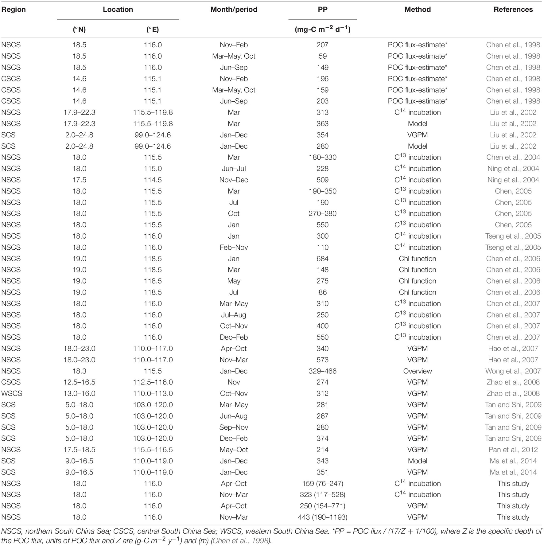
Table 1. Integrated primary production in the euphotic zone (PP) based on selected studies conducted in the South China Sea.

Remote sensing has made it possible to conduct large-scale PP monitoring over extended durations; however, most existing sensing technology is limited to the upper ocean and there is little evidence supporting the assumption of an exponential decrease in PP as a function of depth (Buitenhuis et al., 2013; Shih et al., 2020b). In the current study, we employed data obtained in the SEATS time-series study to elucidate long-term variations in PP_{in situ} under the prevailing monsoon system. We also looked for discrepancies between satellite-based and in situ observations, which could potentially influence PP estimates derived using the VGPM algorithm.

Materials and Methods

In situ Observation

A total of 44 in situ observations were conducted at the SEATS site (18 °N, 116 °E) at regular intervals between 1998 and 2016. These expeditions involved hydrographic seawater sampling and biogeochemical field experiments using research vessels (RV; Ocean Researcher I, Ocean Researcher III, and Fishery Researcher I) (Karl et al., 2003; Wong et al., 2007). On-deck incubation of PP in accordance with ¹⁴C protocols was also conducted during 20 of 25 expeditions between 2003 and 2016 (Figure 1). Conductivity–temperature–depth (CTD) (SBE9/11, SeaBird) and quantum scalar irradiance (QSP-200L, Biospherical) were, respectively, used to obtain vertical profiles of temperature and underwater photosynthetically available radiation (PAR). A Biospherical instrument (QSR-240) was used to obtain daily PAR measurements (i.e., daily surface light intensity). In that study, Z_eu was defined as the depth at which underwater PAR reached 1%. The mixed layer depth (MLD) was defined as the deepest depth at which the temperature was 0.8°C lower than at the surface (Kara et al., 2000; Chou et al., 2006).

FIGURE 1

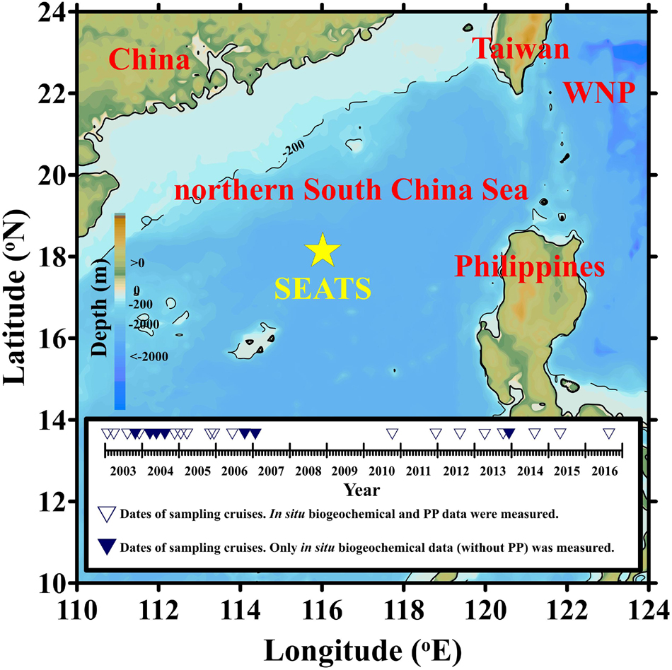
Figure 1. Location of the South East Asian Time-series Study (SEATS) site. Inner box represents the date of cruises conducted at the SEATS site. Major and minor ticks, respectively, exhibit intervals of years and months. WNP refers to the western North Pacific.

Seawater samples were collected at discrete depths to determine Chl concentrations and PP values. Briefly, 2L seawater samples were filtered using 47-mm GF/F filters before obtaining Chl concentrations (via acidification) using a Turner 10-AU-005 fluorometer (Gong et al., 2003; Shiah et al., 2003). PP was measured using the ¹⁴C assimilation method (Parsons et al., 1984) following incubation under an artificial light source (2,000 μE m^–2 s^–1 with full spectrum from 350 to 2450 nm, similar to sunlight) for ∼3 h in a proprietary isolation container using flowing surface seawater for cooling. Following incubation and acidification (0.5 N HCl), radioactive substances collected in 25-mm GF/F filters were transported to a lab for quantification using a scintillation counter (Packard 2200) (Gong et al., 2003; Shiah et al., 2003; Lai et al., 2014). Finally, PP was calculated via trapezoidal integration (i.e. integrated from surface to 1% PAR). Note that SST, Chl and PP measurements from the Ocean Data Bank (Ministry of Science and Technology, Taiwan¹) were used to compensate for deficiencies in in situ observations. Some of the hydrographic records (i.e., SST) and biogeochemical parameters (i.e., PP, Chl_s) of May–October from 2003 to 2006 have been present by Pan et al. (2012).

Remote Sensing Observation

Between 2003 and 2016, the daily data of level-3 products were obtained using a passive ocean color MODerate resolution Imaging Spectroradiometer (Aqua sensor; MODIS-Aqua) with spatial resolution of 4 km for the region covering 17.5–18.5°N and 115.5–116.5°E. We also collected PP_VGPM, SST, E₀, K_d, and Chl_s values from the Environmental Research Division’s Data Access Program (ERDDAP), National Oceanic and Atmospheric Administration, Department of Commerce, U. S.². Note that 8-day composite data were applied in situations where daily observations were missing. Note also that PP_VGPM values obtained from ERDDAP were estimated using VGPM developed by Behrenfeld and Falkowski (1997).

Plausible deviations between PP_VGPM and PP_{in situ} were examined by comparing data obtained from satellites vs. data obtained in situ, including i.e., SST_sate, (${\text{P}}_{\text{opt}}^B$)_sate, E_0–sate, [E₀/(E₀+4.1)]_sate, K_d–sate, Z_eu–sate, Chl_s–sate; SST_{in situ}, (${\text{P}}_{\text{opt}}^B$)_{in situ}, E_{0–in situ}, [E₀/(E₀+4.1)]_{in situ}, K_{d–in situ}, Z_{eu–in situ}, Chl_{s–in situ}. Note that this analysis was conducted using the VGPM algorithm proposed by Behrenfeld and Falkowski (1997) (with far fewer input variables), as Equation 2–1:

$$\begin{array}{c}\text{PP}=0.66125\times {\text{P}}_{\text{opt}}^{\text{B}}\times [{\text{E}}_0/({\text{E}}_0+4.1)]\times {\text{Z}}_{\text{eu}}\times \hfill \\ {\text{Chl}}_{\text{s}}\times {\text{D}}_{\text{irr}}\hfill \end{array}(\mathrm{2-1})$$

where the D_irr refers to the photoperiod. Z_eu was estimated from the average K_d of the water column (Behrenfeld and Falkowski, 1997 and references therein).

${\text{P}}_{\text{opt}}^B$ was computed using the empirical equation proposed by Behrenfeld and Falkowski (1997), as Equation 2–2, where T refers to the incubation temperature measured in the deck incubator as SST_{in situ} or SST_sate. In cases where SST exceeded 28.5°C, a constant value of 4.0 mg-C mg-Chl^–1 h^–1 was taken as ${\text{P}}_{\text{opt}}^B$ (Behrenfeld and Falkowski, 1997; Hu et al., 2014).

$$\begin{array}{c}{\text{P}}_{\text{opt}}^{\text{B}}=-3.27\times {10}^{-8}{\text{T}}^7+3.4132\times {10}^{-6}{\text{T}}^6-1.348\times \hfill \\ {10}^{-4}{\text{T}}^5+2.462\times {10}^{-3}{\text{T}}^4-0.0205{\text{T}}^3+0.0617{\text{T}}^2+\hfill \\ 0.2749\mathrm{T}+1.2956\hfill \end{array}(\mathrm{2-2})$$

To evaluate the impact of monsoonal force on time-series variations, all data sets were divided into two groups: SW-monsoon (SWM, Apr. to Oct., including inter-monsoons of Apr and Oct) and NE-monsoon (NEM, Nov. to Mar). Variations between satellite-based observations and in situ measurements were examined by averaging all relevant values and reporting them as mean ± standard deviation (SD). Linear regression was used to assess relationships between any two of the variables. The t-tests were used to compare sets of observations with the significance level set at p = 0.10.

Results

Time-Series Distributions: PP, SST, E₀, K_d, and Chl_s

As shown in Figure 2A, PP_{in situ} was ∼2.0 times higher during the NEM (117–528, average = 323 ± 134 mg-C m^–2 d^–) than during the SWM (76–247, average = 159 ± 58 mg-C m^–2 d^–1) (Table 2). PP_VGPM values between 2003 and 2016 were as follows: SWM was 250 ± 36; 154–771 mg-C m^–2 d^–1 and NEM was 443 ± 142; 190–1,153 mg-C m^–2 d^–1 (Figure 2A). Note that PP_VGPM during the NEM was ∼1.8 times higher than during the SWM (p < 0.01) (Table 2). The differences in PP_{in situ} and PP_VGPM between the NEM and SWM are in line with those reported by Ning et al. (2004); Chen (2005), and Hao et al. (2007), all of which were obtained from the same area of the SCS using different methods (Table 1). PP_VGPM exhibited monsoonal variations resembling the curve derived from PP_{in situ}; however, the magnitudes were 37% higher during the NEM and 57% higher during the SWM. On average, PP_{in situ} estimates were ∼50% lower than PP_VGPM estimates, regardless of monsoon.

FIGURE 2

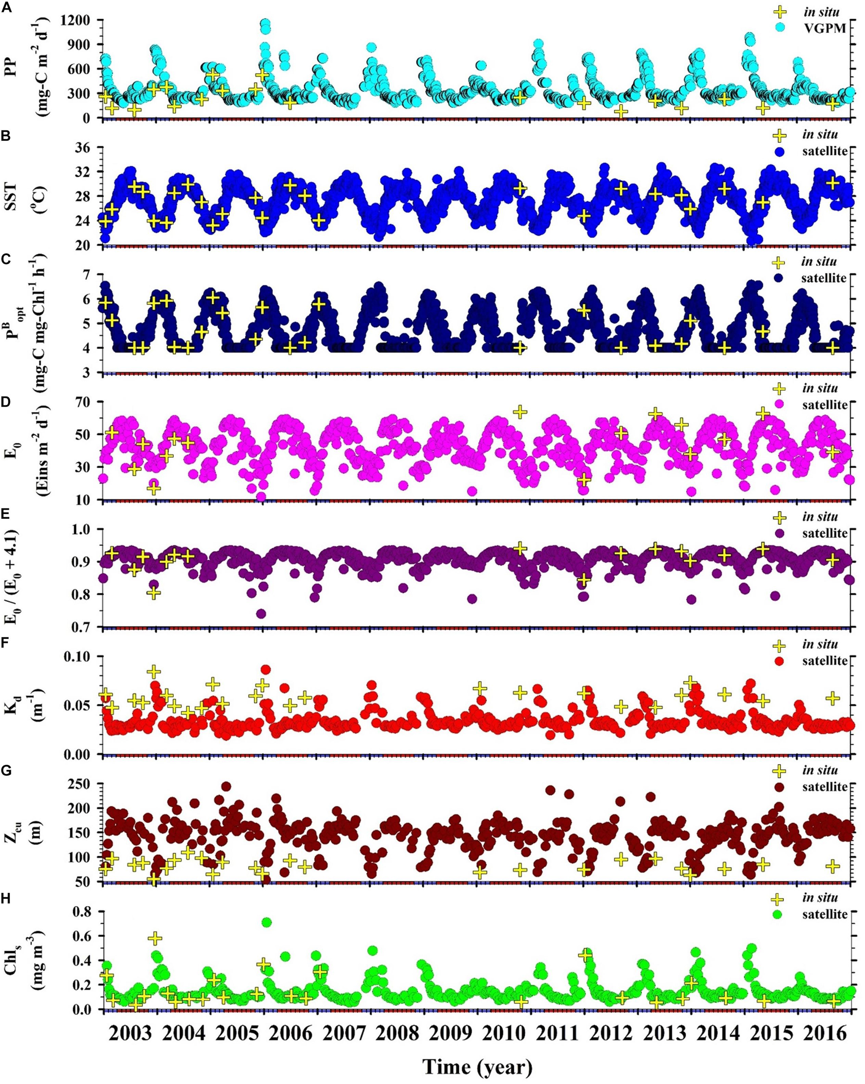
Figure 2. Time-series distributions of satellite-based (circles) and in situ measurements obtained at the SEATS site (crosses): (A) Euphotic zone integrated primary production, PP; (B) sea surface temperature, SST; (C) optimal carbon fixation rate, ${\text{P}}_{\text{opt}}^{\text{B}}$; (D) sea surface daily light intensity, E₀; (E) E₀/(E₀+4.1) ratio; (F) light diffuse attenuation coefficient, K_d; (G) depth of euphotic zone, Z_eu; (H) sea surface Chl, Chl_s. Red and blue colors on the horizontal axis, respectively, indicate SWM (Apr–Oct) and NEM (Nov–Mar).

TABLE 2

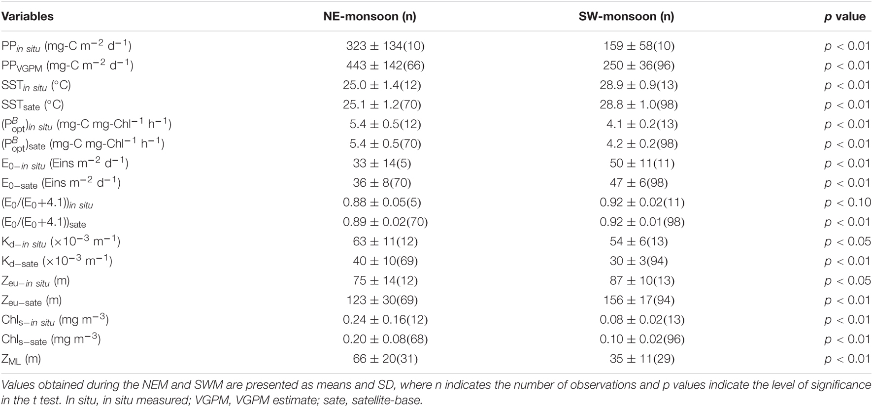
Table 2. Summary of euphotic zone PP (PP) and its relevant variables in the current study conducted at the SEATS: SST, ${\text{P}}_{\text{opt}}^B$, E₀, E₀/(E₀+4.1), K_d, Z_eu, Chl_s and Z_ML.

The lowest SST_{in situ} (25.0 ± 1.4°C) and SST_sate (25.1 ± 1.2°C) values were obtained under the prevailing NEM during the cold season. The highest SST_{in situ} (28.9 ± 0.9°C) and SST_sate (28.8 ± 1.0°C) values were obtained under the prevailing SWM during the warm season (Table 2). The low SST values recorded during the NEM can be attributed to the combined dynamics of NEM-driven vertical mixing of seawater and reduced solar radiation (Tseng et al., 2005; Zhou et al., 2020). By contrast, the ${\text{P}}_{\text{opt}}^{\text{B}}$ showed a synchronous but opposite distribution (Figures 2B,C). The (${\text{P}}_{\text{opt}}^{\text{B}}$)_{in situ} and (${\text{P}}_{\text{opt}}^{\text{B}}$)_sate values computed from SST for the NEM, respectively, ranged from 4.4 to 6.1 and 4.0 to 6.6 mg-C mg-Chl^–1 h^–1, and the average value was the same (5.4 ± 0.5 mg-C mg-Chl^–1 h^–1). The (${\text{P}}_{\text{opt}}^{\text{B}}$)_{in situ} and (${\text{P}}_{\text{opt}}^{\text{B}}$)_sate values for the SWM, respectively, ranged from 4.0 to 4.4 and 4.0 to 6.0 mg-C mg-Chl^–1 h^–1, with mean ${\text{P}}_{\text{opt}}^{\text{B}}$ values of 4.1 ± 0.2 and 4.2 ± 0.2 mg-C mg-Chl^–1 h^–1 (Table 2).

E_{0–in situ} and E_0–sate values in the SWM (50 ± 11 and 47 ± 6 Eins m^–2 d^–1) were higher than those in the NEM (33 ± 14 and 36 ± 8 Eins m^–2 d^–1) (see Figures 2D,E and Table 2). From the perspective of variables in the VGPM algorithm, E₀/(E₀+4.1) ratios varied little between the in situ measurement and satellite-based observation. The variable of [E₀/(E₀+4.1)] thereby seemed not an important parameter to influence the PP level. Z_eu was estimated using the expression of –ln(0.01)/K_d (Kirk, 1994; Behrenfeld and Falkowski, 1997), which led to a reversal of monsoonal K_d and Z_eu distributions (see Figures 2F,G). The mean Z_{eu–in situ} was deeper during the SWM than during the NEM (87 ± 10 and 75 ± 14 m, respectively). The Z_eu–sate as well as the Z_{eu–in situ} presented similar trends between SWM and NEM (156 ± 17 and 120 ± 30 m, respectively) (Table 2). Z_eu values were shallower in the NEM than in the SWM, due perhaps to reduced light penetration resulting from more abundant biomass in the water column (Chen, 2005; Tseng et al., 2005; Chen et al., 2008).

Figure 2H presents long-term temporal variations in Chl_s. In situ measurements and satellite-based observations revealed a distinct NEM maximum (0.24 ± 0.16 and 0.20 ± 0.08 mg m^–3, respectively) and a SWM minimum (0.08 ± 0.02 and 0.10 ± 0.02 mg m^–3, respectively). Chl_{s–in situ} and Chl_s–sate concentrations were, respectively, 0.07 to 0.58 and 0.09 to 0.71 mg m^–3 during the NEM, and were, respectively, 0.04 to 0.11 and 0.05 to 0.43 mg m^–3 during the SWM. For the same location, our observations were close to the data reported by Chen (2005) and Tseng et al. (2005). The SWM minimum Chl_s values in the current study were nearly the same as those reported in the oligotrophic ocean time-series studies at HOT (Hawaii Ocean Time-Series) and BATS (Bermuda Atlantic Time-Series Study) during the summer (0.05 mg m^–3); however, NEM values at SEATS exceeded the winter maximum at HOT and BATS (0.1 and 0.3 mg m^–3, respectively) (Karl et al., 2003). The high NEM maximum at SEATS may perhaps be explained by an increase in phytoplankton biomass (particularly larger sizes of >3 μm), which was stimulated by the deepening Z_ML (Table 2). The deeper nutrient-rich water was then efficiently transported to the upper surface water under the influence of NEM given that the nutrient-cline depth was shallower in SCS than in other oceans (Chen, 2005; Tseng et al., 2005).

Monthly Variations in PP, SST, E₀, K_d and Chl_s

The PP_VGPM values in this study are in good agreement with PP_{in situ} in terms of amplitude as well as phase. Overall, we observed a maximum PP_{in situ} of 394 ± 190 in January (NEM) and a minimum of 143 ± 70 mg-C m^–2 d^–1 in August (SWM) (Figure 3A). The magnitude of PP_VGPM was higher than the values obtained using in situ measurements; however, the trend over a span of 12 months was similar, with a pronounced NEM peak 619 ± 113 mg-C m^–2 d^–1 in January and the lowest SWM value of 230 ± 28 mg-C m^–2 d^–1 in September. These results are similar to those reported by other researchers for same area using different methods, such as the particulate organic carbon flux re-calculation (NEM: 207, SWM: 149 mg-C m^–2 d^–1) (Chen et al., 1998); on-deck C¹⁴ incubation (NEM: 300–509, SWM: 110–228 mg-C m^–2 d^–1) (Ning et al., 2004; Tseng et al., 2005); on-deck C¹³ incubation (NEM: 190–550, SWM: 190–280 mg-C m^–2 d^–1) (Chen, 2005; Chen et al., 2007), and Chl empirical function (NEM: 148–684, SWM: 86–275 mg-C m^–2 d^–1) (Chen et al., 2006; Table 1).

FIGURE 3

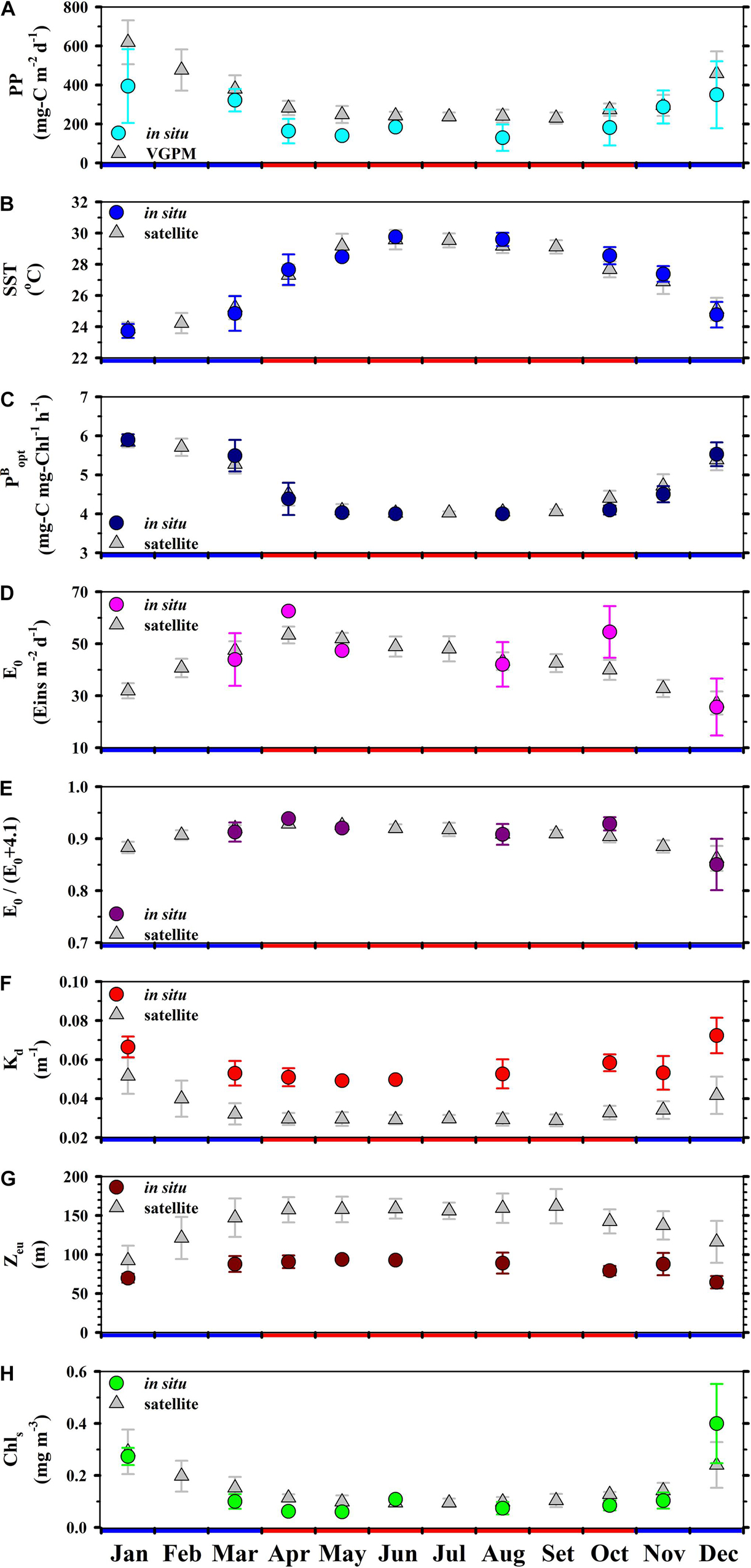
Figure 3. Monthly averages (±1 SD) of (A) PP, (B) SST, (C) ${\text{P}}_{\text{opt}}^{\text{B}},$ (D) E₀, (E) E₀/(E₀+4.1), (F) K_d, (G) Z_eu, (H) Chl_s at the SEATS site. Circles and triangles, respectively, represent in situ measurements and satellite-based observations. Red and blue colors on the horizontal axis, respectively, indicate SWM (Apr–Oct) and NEM (Nov–Mar).

We observed opposing trends between monthly SST and the corresponding ${\text{P}}_{\text{opt}}^B$. The highest (${\text{P}}_{\text{opt}}^B$)_{in situ} values (5.9 mg-C mg-Chl^–1 h^–1) were observed in January and the lowest (4.0 mg-C mg-Chl^–1 h^–1) were observed in August. The (${\text{P}}_{\text{opt}}^B$)_sate values converted from SST_sate (5.8 and 4.0 mg-C mg-Chl^–1 h^–1 in January and June, respectively) were nearly identical to those for the same time slots obtained via in situ measurements (Figures 3B,C). The highest mean monthly E_{0–in situ} in April (63 ± 0 Eins m^–2 d^–1) was higher than the highest mean monthly E_0–sate (53 ± 3 Eins m^–2 d^–1). Overall, E_{0–in situ} and E_0–sate levels in December were very similar (∼26 and ∼27 Eins m^–2 d^–1, respectively). Based on E_{0–in situ}, the highest E₀/(E₀+4.1)_{in situ} ratio (0.94) occurred in April and the lowest E₀/(E₀+4.1)_{in situ} ratio (0.85) occurred in December. E₀/(E₀+4.1)_sate values of 0.93 in April and 0.86 in December were similar with the E₀/(E₀+4.1)_{in situ} values (Figures 3D,E). As for parameterization, it appears that ${\text{P}}_{\text{opt}}^B$ and E₀/(E₀+4.1) values had little influence on VGPM results (PP), regardless of whether the values were obtained from in situ measurements or satellite-based observation.

We did not observe large monsoonal variations in K_{d–in situ} and K_d–sate; however, the highest K_{d–in situ} (0.072 ± 0.009 m^–1) was obtained in December and the highest K_d–sate (0.052 ± 0.009 m^–1) was obtained in January. These high K_d values resulted in a shallower Z_{eu–in situ} (64 ± 8 m) and Z_eu–sate (92 ± 19 m), compared to the values converted from the K_{d–in situ} (0.053 ± 0.007 m^–1) for August (Z_{eu–in situ} = 89 ± 13 m) and the K_d–sate (0.029 ± 0.003 m^–1) for September (Z_eu–sate = 162 ± 22 m) (Figures 3F,G). The shallow Z_eu observed in December and January can be attributed mainly to an increase in phytoplankton biomass that reduces the light penetration in that region during the NEM (Chen, 2005; Tseng et al., 2005; Chen et al., 2008).

Figure 3H presents temporal variations in Chl_{s–in situ} and Chl_s–sate. Conspicuously high Chl_{s–in situ} values were observed in December (0.40 ± 0.15 mg m^–3) and high Chl_s–sate values were observed in January (0.29 ± 0.09 mg m^–3). The high Chl_s values observed throughout the NEM were triggered by the monsoonal force, which stimulated phytoplankton photosynthesis, thereby increasing the phytoplankton abundance or enriching the area with Chl_s from subsurface waters (Liu et al., 2002; Tseng et al., 2005). The drop in Chl_{s–in situ} and Chl_s–sate values to nearly < 0.10 mg m^–3 during the SWM has previously been reported in studies focusing on the same region of the SCS (Liu et al., 2002; Chen, 2005; Tseng et al., 2005; Shih et al., 2020a). Similar findings were also recorded in oligotrophic time-series studies, such as HOT and BATS (Karl et al., 2003).

Relationships Among of PP, SST, E₀, K_d and Chl_s in in situ Measurements and Satellite-Based Observations

PP_{in situ} was generally lower than PP_VGPM; however, we observed a significantly positive correlation between these two parameters; i.e., slope = 0.70, r² = 0.42, p < 0.01 (Figure 4A). This clearly indicates the feasibility of the VGPM for predictions; however, tuning would be required for the study area. As shown in Figure 4, we identified significantly positive correlations between PP_{in situ} and PP_VGPM as well as their respective variables SST, E₀, K_d and Chl_s. As indicated by high r² and low p values with slopes close to 1, the most significant correlations were found in SST and E₀ (Figures 4C–F) : SST (slope = 0.92, r² = 0.92, p < 0.01) and E₀ (slope = 0.62, r² = 0.58, p < 0.01). Taken together, these results indicate that SST_sate and E_0–sate were the variables most strongly correlated with SST_{in situ} and E_{0–in situ}, providing the most accurate estimates of PP when using the VGPM. As indicated by the 1:1 lines in Figures 4B,G,H, the parameters with the greatest variability in terms of slope were Chl_s (slope = 0.41, r² = 0.74, p < 0.01) and K_d (slope = 0.59, r² = 0.50, p < 0.01). This suggests Chl_s–sate and K_d–sate could potentially bias PP estimates obtained using the VGPM.

FIGURE 4

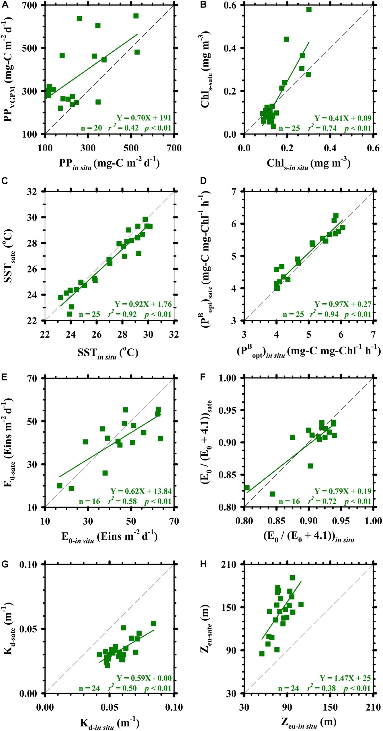
Figure 4. Linear relationships among satellite-based observations and in situ measurements. Panels (A–H) are PP, Chl_s, SST, ${\text{P}}_{\text{opt}}^{\text{B}}$ (estimated from SST), E₀, E₀/(E₀+4.1) ratio, K_d, and Z_eu (estimated from K_d), respectively. Diagonals in panels (A–H) are 1:1 lines.

The fact that the regression line between PP_VGPM and PP_{in situ} lies above the 1:1 line indicates that PP_VGPM estimates exceeded PP_{in situ}. When using the VGPM to estimate PP, the two main variables are ${\text{P}}_{\text{opt}}^B$ and E₀/(E₀+4.1), derived from in situ measurements and satellite-based observations of SST (SST_{in situ} and SST_sate) and E₀ (E_{0–in situ} and E_0–sate). Between SST_{in situ} and SST_sate as well as between E_{0–in situ} and E_0–sate, we observed nearly linear relationships (i.e., close to the 1:1 diagonal). This suggests that ${\text{P}}_{\text{opt}}^B$ and E₀/(E₀+4.1) were not scaling variables governing the magnitude of PP in this study. Influences derived from these two variables [${\text{P}}_{\text{opt}}^B$, E₀/(E₀+4.1)] of the both methods on calculated results were less than 1%. By contrast, the correlations between Chl_{s–in situ} and Chl_s–sate, and Z_{eu–in situ} and Z_eu–sate (converted from K_{d–in situ} and K_d–sate, respectively) had a pronounced impact on VGPM PP estimates. If we considered only the difference between Chl_{s–in situ} and Chl_s–sate, then PP values estimated using VGPM would be slightly higher (∼ 5%, depended on the given case) than those obtained using in situ measurements. If we considered only the difference between Z_{eu–in situ} and Z_eu–sate, then PP values estimated using VGPM would be apparently 1.72-fold higher than those obtained using in situ measurements.

Discussion

Uncertainty in Estimating PP Due to Differences Between Chl_{s–in situ} and Chl_s–sate as Well as Z_{eu–in situ} and Z_eu–sate: Implications

Our analysis of revealed a number of potential uncertainties pertaining to PP estimation using the VGPM algorithm. Most of the discrepancies were due primarily to differences between Z_{eu–in situ} and Z_eu–sate as well as between Chl_{s–in situ} and Chl_s–sate. Overall, the product of Z_eu and Chl_s (i.e., the phytoplankton inventory in the euphotic zone), suggests that the base assumption of vertically distributed standing stock biomass in low latitude waters (SCS) may perhaps be erroneous. If so, then it will be necessary to reformulate methods for the prediction of biomass standing stocks when implementing the VGPM algorithm (Ning et al., 2004; Hill and Zimmerman, 2010).

The fundamental structure of the VGPM is based on a relationship between integrated phytoplankton biomass in the euphotic zone and Chl_s (Behrenfeld and Falkowski, 1997; Hill and Zimmerman, 2010). Thus, obtaining accurate estimates of PP by comparing PP_{in situ} and PP_VGPM results depends on reliable estimates of the integrated phytoplankton biomass in the euphotic zone. However, passive satellites recording the color of the ocean surface are unable to elucidate the situation at arbitrary depths below the surface (Hill and Zimmerman, 2010; Shih et al., 2020b). Contrary to the assumption that Chl decreases exponentially with depth, most observations in the SCS revealed that the subsurface Chl maximum (SCM) was often found at great depths (Liu et al., 2002; Chen, 2005; Shih et al., 2020a, b). This makes it very difficult or even impossible to estimate the integrated biomass in the euphotic zone simply as a product of Z_eu and Chl_s. Enhancing the reliability of the VGPM requires that we increase the number of PP_{in situ} observations and the corresponding variables in order to improve the correlation between our assumptions pertaining to phytoplankton integrated biomass and actual measurements obtained in the field. This is particularly important in phytoplankton populations, dynamics and assemblages in specific locations under specific conditions (Hill and Zimmerman, 2010; Shih et al., 2015, 2020b). Only by increasing the number of observations and enhancing our analysis of water composition will it be possible to reduce the uncertainty associated with Z_eu and Chl_s in estimating PP using the VGPM.

The mean PP in the euphotic zone (PP/Z_eu, mg-C m^–3 d^–1) presented a positive linear relationship between (PP_VGPM/Z_eu–sate) and (PP_{in situ}/Z_{eu–in situ}); i.e., slope: 0.51, r² = 0.39, p < 0.01 (Figure 5A). Higher values were observed during the NEM (4.7 ± 2.4 and 3.8 ± 2.2 mg-C m^–3 d^–1 of PP_{in situ}/Z_{eu–in situ} and PP_VGPM/Z_eu–sate, respectively) and lower values were observed during the SWM (1.9 ± 0.8 and 1.7 ± 0.4 mg-C m^–3 d^–1 of PP_{in situ}/Z_{eu–in situ} and PP_VGPM/Z_eu–sate, respectively). The slope of 0.51 for PP_VGPM/Z_eu–sate and PP_{in situ}/Z_{eu–in situ} was lower than that of PP_VGPM and PP_{in situ} (slope = 0.70), such that most data fell on the right side of the 1:1 line. Ratios of PP_VGPM/Z_eu–sate were nearly 20% lower than those of PP_{in situ}/Z_{eu–in situ}, indicating that Z_eu–sate was deeper than Z_{eu–in situ}, particularly during the SWM. This also indicates that the VGPM parameter Z_eu–sate indeed substantially affected PP estimates in this study. It has been proposed that satellite-based K_d values have to be calibrated against the zenith solar angle during the data processing in accordance with the methods outlined by Lee et al. (2005) and Li et al. (2015). However, users may not to confirm the processing from the downloaded or retrieved satellite-based products of PP and its relevant variables.

FIGURE 5

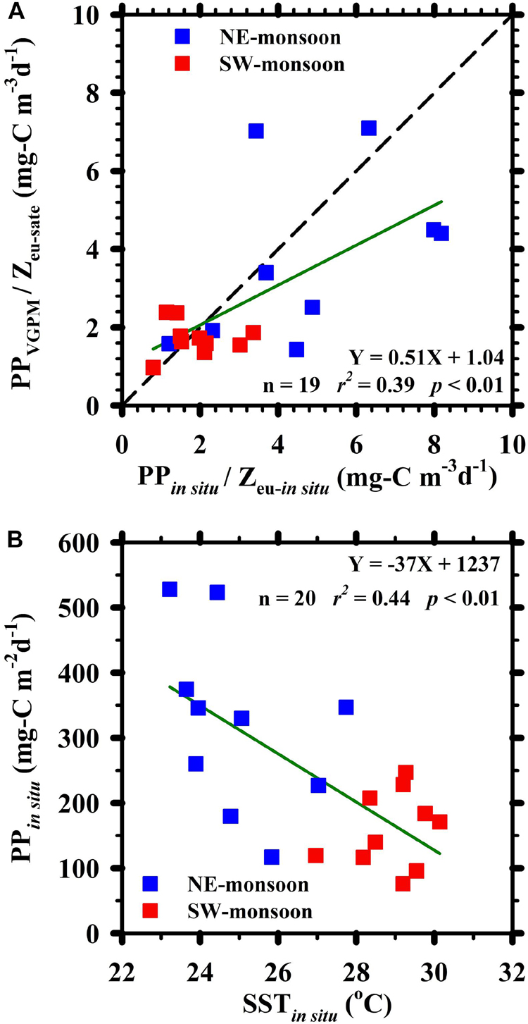
Figure 5. (A) Relationship between satellite-based observations of (PP_VGPM / Z_eu–sate) and in situ measurements of (PP_{in situ} / Z_{eu–in situ}) ratios; (B) relationship between PP_{in situ} and SST_{in situ}. Red and blue symbols, respectively, indicate observations made during the SW-monsoon and NE-monsoon. The diagonal in panel (A) is 1:1 line.

The significant linear correlation between (${\text{P}}_{\text{opt}}^B$)_sate and (${\text{P}}_{\text{opt}}^B$)_{in situ} (slope = 0.97, r² = 0.94, p < 0.01; Figure 4D) is simply a reflection of the relationship between the two SST records, resulting from the fact that ${\text{P}}_{\text{opt}}^B$ is computed as a function of SST (i.e., a seventh-order polynomial, Equation 2–2) (Behrenfeld and Falkowski, 1997). Thus, any potential deviations between SST and ${\text{P}}_{\text{opt}}^B$ had only a negligible influence on PP estimates obtained using VGPM. Many studies have nevertheless concluded that the accuracy of VGPM-based estimates of PP are poor, when using the 7th order polynomial of SST (Equation 2–2) to calculate the input of ${\text{P}}_{\text{opt}}^B$ (Mizobata and Saitoh, 2004; Kameda and Ishizaka, 2005; Yamada et al., 2005; Siswanto et al., 2006; Ishizaka et al., 2007; Tang et al., 2008; Tang and Chen, 2016).

Researchers have reported that much of the uncertainty in estimating PP_VGPM is related to the computation of ${\text{P}}_{\text{opt}}^B$ under the effects of phytoplankton physiology, growth conditions, abundance, size, and productivity (Gong and Liu, 2003; Kameda and Ishizaka, 2005; Yamada et al., 2005). It has been suggested that ${\text{P}}_{\text{opt}}^B$ is influenced by SST as well as E₀ and various biological parameters, such as Chl concentration. ${\text{P}}_{\text{opt}}^B$ represents an optimal daily carbon fixation rate in the water column previously described as a 7th order polynomial of SST, however, when SST exceeds 28.5°C, ${\text{P}}_{\text{opt}}^B$ remains fixed at a constant 4 mg-C mg-Chl^–1 h^–1 (Behrenfeld and Falkowski, 1997; Mizobata and Saitoh, 2004), indicating that ${\text{P}}_{\text{opt}}^B$ tends to be underestimated when SST exceeds 28.5°C. In low-latitude regions of the SCS, the constant ${\text{P}}_{\text{opt}}^B$ mentioned above usually occurred in late spring, summer, and early fall, during which SST_{in situ} and SST_sate both exceeded 28.5°C. This increased the margin between actual PP values and the estimates obtained by inputting ${\text{P}}_{\text{opt}}^B$ derived using SST_{in situ} or SST_sate. The reliability of ${\text{P}}_{\text{opt}}^B$ estimates obtained using the VGPM seventh-order polynomial SST algorithm is not universally applicable (temporally or spatially). This has prompted oceanographers to tune existing methods or devise new methods for the precise estimation of ${\text{P}}_{\text{opt}}^B$, especially for ocean water at low latitudes.

Our results reveal that the satellite-derived primary production (e.g., PP_VGPM) may significantly affect global carbon export flux to deep waters, but what is the overall significance and impact of these PP values on POC fluxes? For example, Dunne et al. (2005) used the empirical model expression (Equation 4–1) to estimate carbon flux (or sequestration) in oceans. PP (mg-C m^–2 d^–1), Z_eu (m) and SST (°C) are three major factors affecting the estimated values of POC flux which is almost linearly proportional to PP.

$$\begin{array}{c}\mathrm{POC}\mathrm{flux}=PP\times [-{0.0101}^{\circ }{\text{C}}^{-1}\times SST+0.0582\times \hfill \\ \ln \left({\displaystyle \frac{PP}{Z_{\text{eu}}}}\right)+0.419]\hfill \end{array}(\mathrm{4-1})$$

According to the expression 4–1, the POC fluxes estimated from in situ measurements (PP_{in situ}, SST_{in situ} and Z_{eu–in situ}) of Hung et al. (2000); Hung and Gong (2007), and Shih et al. (2015) were from 12 to 319 mg-C m^–2 d^–1, an average of 20% less than the trap POC fluxes (25–274 mg-C m^–2 d^–1) (Figure 6). As described above, the inputs of SST_{in situ} and Z_{eu–in situ} to the expression were fixed, the PP_{in situ} was replaced by the PP_VGPM, an average difference between estimated and trap POC fluxes (estimated POC flux: 16–781 mg-C m^–2 d^–1) was a factor of 2. It has been suggested that the uncertainty of these POC fluxes is quite large if satellite-based PP is used to estimate carbon sequestrations in oceans. If the discrepancy between in situ measurements and satellite-based observations of PP can be diminished and the reliance on them (e.g., PP_VGPM) can be increased, it is to dedicate the potential importance and goal of the present study.

FIGURE 6

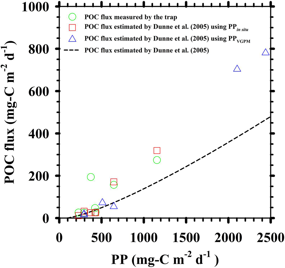
Figure 6. A comparison of the difference between in situ trap measured and estimated POC fluxes. The estimated POC fluxes were computed according to the empirical model expression revealed by Dunne et al. (2005). The dashed line represented the proportional relationship of estimated POC flux and PP. The PP_{in situ} and PP_VGPM were also exerted on the expression to estimate POC fluxes (red square and blue triangle, respectively). In situ measurements of PP_{in situ} and trap measured POC fluxes (green circle) were based on Hung et al. (2000); Hung and Gong (2007), and Shih et al. (2015).

Impact of Global Warming on in situ Observations

In both the Atlantic and Pacific oceans, increased phytoplankton biomass is observed at low latitudes during the boreal warm season. Other than equatorial upwelling, there are no other conspicuous seasonal trends in biogeochemical activities (Dandonneau et al., 2004). In the Arabian Sea, enhanced biogeochemical responses are also observed at low latitudes during the SWM (Banse and English, 2000). In this study, long-term and monthly variations in PP_{in situ} and PP_VGPM demonstrated influential monsoonal system at the SEATS (Figures 2, 3 and Table 2). The concurrence of low SST, deep Z_ML, high Chl_s, shallow Z_eu, and increased PP suggest that increased phytoplankton biomass or specific phytoplankton communities dominating were triggered during the NEM. It has been reported that the average nitrate+nitrite (N+N) concentration, one of the key nutrients for phytoplankton growth in the SCS, in the MLD in the seasons of NEM (0.1–0.3 μM) is ∼10 times higher than of SWM (∼0.03 μM) (Tseng et al., 2005). Moreover, the inventory of N+N and the depth of nitracline in the NEM (30 ± 19 mmol m^–2 and 28–62 m, respectively) have been observed a ∼ 4.5 fold higher and a ∼ 25–50% shallower than those reported in the SWM (7 ± 4 mmol m^–2 and 52–82 m, respectively) (Chen, 2005; Shih et al., 2020a). Evidences of abundant nutrient (e.g., N+N) and shallow nitracline depth favoring biological activities, imply that the growth of phytoplankton communities and associated photosynthesis were affected mainly by vertical advection providing inorganic nutrients from deeper waters, under the NEM system prevailing in the SCS (Liu et al., 2002; Bai et al., 2018; Chen et al., 2020; Zhou et al., 2020).

The global decrease in PP is particularly pronounced in high-latitude waters, which lose roughly 2,000 Mt-C y^–1 (Mt = 10¹² g), accounting for a 70% decline in carbon fixation via photosynthesis (Gregg et al., 2003). To compare annually reductions in PP_{in situ} (−11 mg-C m^–2 d^–1 y^–1) vs. the annual PP_{in situ} (241 mg-C m^–2 d^–1; mean PP_{in situ} of NEM and SWM; Table 1), it indicated that the annual reduction in carbon fixation via photosynthesis was ∼ -5% y^–1. Based on the 200 m isobath boundary of oligotrophic waters in the SCS (2.76 × 10¹² m²; Lin et al., 2003), the e-ratios were 5–16% in the SCS (Hung and Gong, 2010; Shih et al., 2019) and the decreased in carbon fixation was roughly 11 Mt-C, thereby accounting for 30–90% of the export production. This suggests a gradual decrease in the efficiency of photosynthetic carbon fixation by phytoplankton. Nevertheless, satellite-based observations do not show the signs of global warming on carbon fixation and sequestration.

Figure 5B illustrates the significantly negative relationship between PP_{in situ} and SST_{in situ} at the SEATS site. The slope of −37 mg-C m^–2 d^–1°C ^–1 was exceptionally close to the −36 mg-C m^–2 d^–1°C ^–1 reported in previous studies (Chen and Chen, 2006; Chen et al., 2007, 2008). Scaling factors related to the increase in SST_{in situ} caused by global changes are extremely complex (Sarmiento et al., 1998; Hung et al., 2010; Bai et al., 2018). Notwithstanding the complexity of factors governing SST_{in situ}, they can still be used to estimate PP values. The differences between daytime and nighttime SST_{in situ} values were statistically insignificant, during the NEM as well as the SWM (one-tail t test: p = 0.15 and 0.24, respectively (Figure 6). We therefore surmise that SST sampling schedules had no effect on the overall results. Furthermore, we observed a strong statistically significant correlation between SST_sate and SST_{in situ} (Figure 4C), indicating the efficacy of SST in estimating PP distributions over a broad horizontal area, regardless of the method used for derivation.

The straightforward relationship between PP_{in situ} and SST_{in situ} is important when seeking to predict PP values and estimate new or export production in euphotic zones. Under the environmental conditions described above, the reduction in carbon fixation due to photosynthesis would be ∼−15% °C^–1, and the decrease in carbon fixation would be roughly 37 Mt-C, thereby accounting for a 1- to 3-fold quantity of export production. The negative correlation between PP_{in situ} and SST_{in situ} in the current study matched the findings observed in mid-latitude tropical/subtropical regions of the Pacific and Atlantic oceans (Chen, 2000; Tilstone et al., 2009), but differed drastically from those reported in high-latitude regions (Kudryavtseva et al., 2018).

Generally speaking, the sampling resolution of in situ time-series is too low to eliminate temporal uncertainty over all timespans. Fortunately, we can use SST_sate to compensate for deficiencies in SST_{in situ} coverage (Bai et al., 2018; Chen et al., 2020). Only one daily SST_sate reading can be obtained at any given location; however, it would be perfectly reasonable to substitute that value with one obtained SST_{in situ}. We observed a statistically significant linear relationship between SST_sate with SST_{in situ} (Figure 4C); however, differences between daytime and nighttime SST_{in situ} measurements did not reach the level of significance (Figure 7). This suggests that SST estimates obtained using either method could be used to assess the influence of temperature on biogeochemical phenomena, such as PP.

FIGURE 7

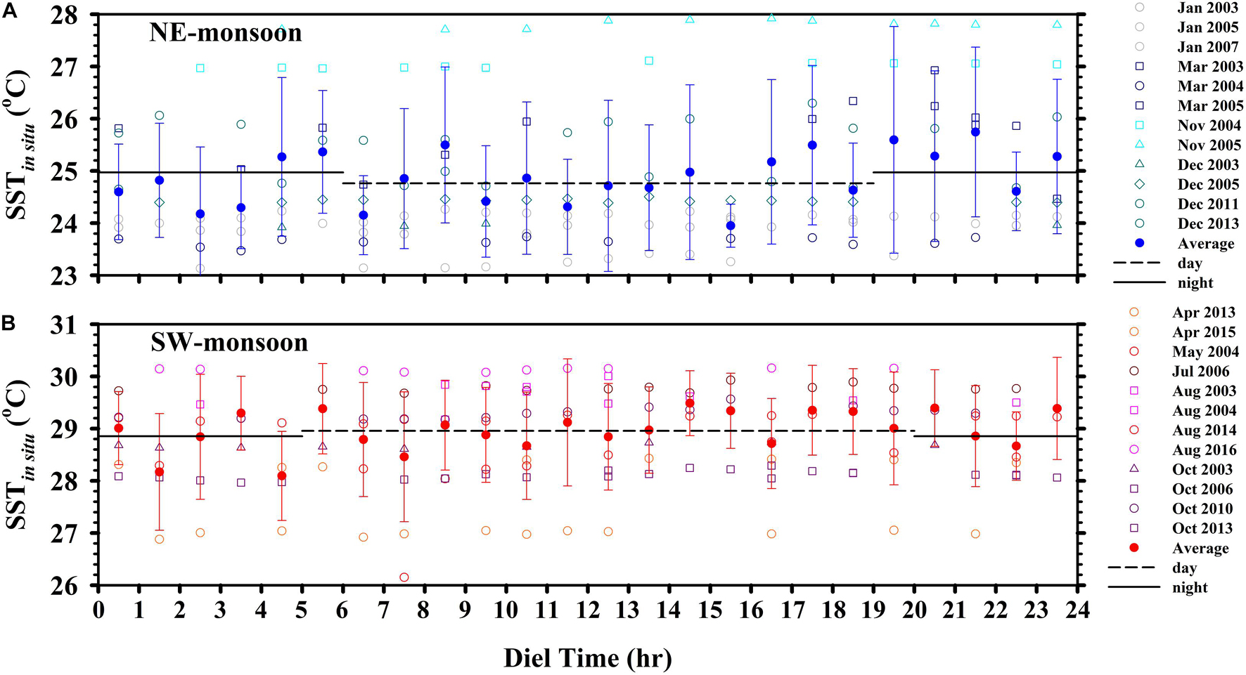
Figure 7. Averaged diel records (±1 SD) of SST during the (A) NE-monsoon and (B) SW-monsoon. Horizontal dashed and solid lines indicate the mean daytime measurements (GMT+8: 06–18 and 05–19 h, NE- and SW-monsoons, respectively) and nighttime measurements (GMT+8: 19–05 and 20–04 h, NE- and SW-monsoons, respectively).

Asynchronous variations between PP_{in situ} and PP_VGPM and their related variables in the VGPM algorithm indicate the following: (1) Satellite-based evaluations depend primarily on the assumption of an exponential decrease in the vertical distribution of PP from the surface to the euphotic zone base. Nonetheless, remote sensing cannot penetrate beyond the surface, and therefore cannot reflect the true vertical distribution of PP at depth (Hung et al., 2010; Buitenhuis et al., 2013; Shih et al., 2013, 2020b). This assumption is the primary cause for uncertainty between PP values obtained from satellite-based observations (i.e., PP_VGPM) and those derived from in situ measurements (i.e., PP_{in situ}). (2) When using satellite-based observations to estimate horizontal PP distributions, mathematical extrapolation/interpolation is commonly used to compensate for gaps in data coverage resulting from cloud coverage, heavy rains, rough seas, extreme weather events, natural episodes, suspended particles, and/or chromophoric dissolved organic matter. Thus, this approach cannot reflect “true” or “in situ” biogeochemistry responses to PP in the oceans. (Boyd and Trull, 2007; Shang et al., 2008; Tang et al., 2008; Hung et al., 2009, 2010; Shih et al., 2020a). For decades, SEATS has been used as a natural laboratory for studies of prolonged environmental changes and reciprocal biogeochemical responses. It is time to tune existing models or develop more reliable models if we are to gain meaningful estimates of biogeochemical phenomena in the oceans. The proposed calibration method aimed at improving PP estimates for the VGPM is expected to enhance our understanding of changes in the SCS.

Summary

Our time-series study (2003 ∼ 2016) at SEATS compared PP estimates based on in situ measurements and those based on the VGPM in the SCS during the NEM and SWM. PP values obtained during the NEM exceeded those obtained during the SWM, which appears to indicate that weather conditions during the cold season are conducive to high PP values. PP_{in situ} values were roughly 50% lower than PP_VGPM values, regardless of the season (NEM or SWM). These discrepancies can be attributed to the satellite-based integrated phytoplankton biomass in the euphotic zone. The discrepancies can be derived as the product of Z_eu and Chl_s, which are two main variables in the VGPM algorithm, especially the impact of difference between in situ and satellite-based Z_eu on the magnitude of PP.

The observed overall decrease in PP_{in situ} can be partially explained by an increase in SST_{in situ}. Our results also showed that SST_sate could be used to predict horizontal PP distributions over extended time scales, based on our observation of a statistically significant relationship between SST_sate with SST_{in situ}. A significantly negative relationship between PP_{in situ} and SST_{in situ} appears to indicate that global changes, such as oceanic warming, could have a negative impact on ocean biogeochemistry in low-latitude regions of the SCS. Nonetheless, further research will be required to assess the influence of global changes on biogeochemical phenomena, particularly in low-latitude waters. The SEATS has been used for decades to assess the sensitivity and resilience of low-latitude oceans to environmental fluctuations. Our analysis of discrepancies between in situ measurements and satellite-based observations could help to guide revisions aimed at enhancing the robustness and reliability of the VGPM in estimating biogeochemical responses. Satellite-based data could be used to expand the spatiotemporal scale of observations and thereby shed light on the actual biogeochemical effects of global environmental changes in low-latitude regions of the SCS.

Data Availability Statement

The original contributions presented in the study are included in the article/supplementary material, further inquiries can be directed to the corresponding author.

Author Contributions

Y-YS, F-KS, and C-CH wrote the manuscript with contributions from W-CC. C-YL, J-HT, Y-SW, and C-CL performed the experiments and created the tables and figures. Y-YS, F-KS, C-CH, W-CC, C-YL, J-HT, Y-SW, C-CL and C-YK reviewed and revised the manuscript. All authors listed have made substantial, direct, and intellectual contribution to the work and approved it for publication.

Funding

This research was supported by the MOST (Ministry of Sciences and Technology, Taiwan) under grant numbers 108-2611-M-012-001, 108-2611-M-110-019-MY3, 109-2611-M-012-001, 109-2740-M-110-001, 110-2611-M-012-002, 110-2740-M-110-001, and 110-2611-M-019-005.

Conflict of Interest

The authors declare that the research was conducted in the absence of any commercial or financial relationships that could be construed as a potential conflict of interest.

Publisher’s Note

All claims expressed in this article are solely those of the authors and do not necessarily represent those of their affiliated organizations, or those of the publisher, the editors and the reviewers. Any product that may be evaluated in this article, or claim that may be made by its manufacturer, is not guaranteed or endorsed by the publisher.

Acknowledgments

We would like to thank the assistance given us by the crews of R/V Ocean Researcher I and R/V Fishery Researcher I. We would also like to thank the unsung heroes and contributors who have contributed to the SEATS program.

Footnotes

1. ^ http://www.odb.ntu.edu.tw/
2. ^ https://coastwatch.pfeg.noaa.gov/erddap/index.html

References

Bai, Y., He, X. Q., Yu, S. J., and Chen, C. T. A. (2018). Changes in the ecological environment of the marginal seas along the Eurasian Continent from 2003 to 2014. Sustainability 10:635. doi: 10.3390/su10030635

CrossRef Full Text | Google Scholar

Balch, W. M., Abbott, M. R., and Eppley, R. W. (1989). Remote sensing of primary production—I. A comparison of empirical and semi-analytical algorithms. Deep Sea Res. A 36, 281–295. doi: 10.1016/0198-0149(89)90139-8

CrossRef Full Text | Google Scholar

Banse, K., and English, D. C. (2000). Geographical differences in seasonality of CZCS-derived phytoplankton pigment in the Arabian Sea for 1978–1986. Deep Sea Res. II 47, 1623–1677. doi: 10.1016/S0967-0645(99)00157-5

CrossRef Full Text | Google Scholar

Behrenfeld, M. J., and Falkowski, P. G. (1997). Photosynthetic rates derived from satellite-based chlorophyll concentration. Limnol. Oceanogr. 42, 1–20. doi: 10.4319/lo.1997.42.1.0001

CrossRef Full Text | Google Scholar

Boyd, P. W., and Trull, T. W. (2007). Understanding the export of biogenic particles in oceanic waters: is there consensus? Prog. Oceanogr. 72, 276–312. doi: 10.1016/j.pocean.2006.10.007

CrossRef Full Text | Google Scholar

Buitenhuis, E. T., Hashioka, T., and Le Quéré, C. (2013). Combined constraints on global ocean primary production using observations and models. Glob. Biogeochem. Cycles 27, 847–858. doi: 10.1002/gbc.20074

CrossRef Full Text | Google Scholar

Campbell, J., Antoine, D., Armstrong, R., Arrigo, K., Balch, W., Barber, R., et al. (2002). Comparison of algorithms for estimating ocean primary production from surface chlorophyll, temperature, and irradiance. Glob. Biogeochem. Cycles 16:1035. doi: 10.1029/2001GB001444

CrossRef Full Text | Google Scholar

Chen, C. C., Shiah, F. K., Chung, S. W., and Liu, K. K. (2006). Winter phytoplankton blooms in the shallow mixed layer of the South China Sea enhanced by upwelling. J. Mar. Syst. 59, 97–110. doi: 10.1016/j.jmarsys.2005.09.002

CrossRef Full Text | Google Scholar

Chen, X., Pan, D., Bai, Y., He X., Chen, C. T. A., Kang, Y., et al. (2015). Estimation of typhoon-enhanced primary production in the South China Sea: a comparison with the Western North Pacific. Cont. Shelf Res. 111, 286–293. doi: 10.1016/j.csr.2015.10.003

CrossRef Full Text | Google Scholar

Chen, C. T. A., Yu, S., Huang, T. H., Lui, H. K., Bai, Y., and He, X. (2020). “Changing biogeochemistry in the South China Sea,” in Changing Asia-Pacific Marginal Seas. Atmosphere, Earth, Ocean & Space, eds C. T. A. Chen and X. Guo (Singapore: Springer), doi: 10.1007/978-981-15-4886-4_12

CrossRef Full Text | Google Scholar

Chen, J., Zheng, L., Wiesner, M. G., Chen, R., Zheng, Y., and Wong, H. K. (1998). Estimations of primary production and export production in the South China Sea based on sediment trap experiments. Chin. Sci. Bull. 43, 583–586. doi: 10.1007/BF02883645

CrossRef Full Text | Google Scholar

Chen, T. Y., Tai, J. H., Ko, C. Y., Hsieh, C., Chen, C. C., Jiao, N., et al. (2016). Nutrient pulses driven by internal solitary waves enhance heterotrophic bacterial growth in the South China Sea. Environ. Microbiol. 18, 4312–4323. doi: 10.1111/1462-2920.13273

PubMed Abstract | CrossRef Full Text | Google Scholar

Chen, Y. L. L. (2000). Comparisons of primary productivity and phytoplankton size structure in the marginal regions of southern East China Sea. Cont. Shelf Res. 20, 437–458. doi: 10.1016/S0278-4343(99)00080-1

CrossRef Full Text | Google Scholar

Chen, Y. L. L. (2005). Spatial and seasonal variations of nitrate-based new production and primary production in the South China Sea. Deep Sea Res. I 52, 319–340. doi: 10.1016/j.dsr.2004.11.001

CrossRef Full Text | Google Scholar

Chen, Y. L. L., and Chen, H. Y. (2006). Seasonal dynamics of primary and new production in the northern South China Sea: the significance of river discharge and nutrient advection. Deep Sea Res. I 53, 971–986. doi: 10.1016/j.dsr.2006.02.005

CrossRef Full Text | Google Scholar

Chen, Y. L. L., Chen, H. Y., Karl, D. M., and Takahashi, M. (2004). Nitrogen modulates phytoplankton growth in spring in the South China Sea. Cont. Shelf Res. 24, 527–541. doi: 10.1016/j.csr.2003.12.006

CrossRef Full Text | Google Scholar

Chen, Y. L. L., Chen, H. Y., Lin, I. I., Lee, M. A., and Chang, J. (2007). Effects of cold eddy on phytoplankton production and assemblages in Luzon strait bordering the South China Sea. J. Oceanogr. 63, 671–683. doi: 10.1007/s10872-007-0059-9

CrossRef Full Text | Google Scholar

Chen, Y. L. L., Chen, H. Y., Tuo, S. H., and Ohki, K. (2008). Seasonal dynamics of new production from Trichodesmium N₂ fixation and nitrate uptake in the upstream Kuroshio and South China Sea basin. Limnol. Oceanogr. 53, 1705–1721. doi: 10.4319/LO.2008.53.5.1705

CrossRef Full Text | Google Scholar

Chou, W. C., Chen, Y. L. L., Sheu, D. D., Shih, Y. Y., Han, C. A., Cho, C. L., et al. (2006). Estimated net community production during the summertime at the SEATS time-series study site, northern South China Sea: implications for nitrogen fixation. Geophys. Res. Lett. 33:L22610. doi: 10.1029/2005gl025365

CrossRef Full Text | Google Scholar

Dandonneau, Y., Deschamps, P. Y., Nicolas, J. M., Loisel, H., Blanchot, J., Montel, Y., et al. (2004). Seasonal and interannual variability of ocean color and composition of phytoplankton communities in the North Atlantic, equatorial Pacific and South Pacific. Deep Sea Res. II 51, 303–318. doi: 10.1016/j.dsr2.2003.07.018

CrossRef Full Text | Google Scholar

Dierssen, H. M. (2010). Perspectives on empirical approaches for ocean color remote sensing of chlorophyll in a changing climate. Proc. Natl. Acad. Sci. U.S.A. 107, 17073–17078. doi: 10.1073/pnas.0913800107

PubMed Abstract | CrossRef Full Text | Google Scholar

Du, C., Liu, Z., Dai, M., Kao, S. J., Cao, Z., Zhang, Y., et al. (2013). Impact of the Kuroshio intrusion on the nutrient inventory in the upper northern South China Sea: insights from an isopycnal mixing model. Biogeosciences 10, 6419–6432. doi: 10.5194/bg-10-6419-2013

CrossRef Full Text | Google Scholar

Dunne, J. P., Armstrong, R. A., Gnanadesikan, A., and Sarmiento, J. L. (2005). Empirical and mechanistic models for the particle export ratio. Glob. Biogeochem. Cycles 19:GB4026. doi: 10.1029/2004GB002390

CrossRef Full Text | Google Scholar

Field, C. B., Behrenfeld, M. J., Randerson, J. T., and Falkowski, P. (1998). Primary production of the biosphere: integrating terrestrial and oceanic components. Science 281, 237–240. doi: 10.1126/science.281.5374.237

PubMed Abstract | CrossRef Full Text | Google Scholar

Friedland, K. D., Stock, C., Drinkwater, K. F., Link, J. S., Leaf, R. T., Shank, B. V., et al. (2012). Pathways between primary production and fisheries yields of large marine ecosystems. PLoS One 7:e28945. doi: 10.1371/journal.pone.0028945

PubMed Abstract | CrossRef Full Text | Google Scholar

Gong, G. C. (1993). Correlation of chlorophyll a concentration and sea tech fluorometer fluorescence in seawater. Acta Oceanogr. Taiwan. 31, 117–126.

Google Scholar

Gong, G. C., and Liu, G. J. (2003). An empirical primary production model for the East China Sea. Cont. Shelf Res. 23, 213–224. doi: 10.1016/S0278-4343(02)00166-8

CrossRef Full Text | Google Scholar

Gong, G. C., Wen, Y. H., Wang, B. W., and Liu, G. J. (2003). Seasonal variation of chlorophyll a concentration, primary production and environmental conditions in the subtropical East China Sea. Deep Sea Res. II 50, 1219–1236. doi: 10.1016/s0967-0645(03)00019-5

CrossRef Full Text | Google Scholar

Gregg, W. W., Conkright, M. E., Ginoux, P., O’Reilly, J. E., and Casey, N. W. (2003). Ocean primary production and climate: global decadal changes. Geophys. Res. Lett. 30:1809. doi: 10.1029/2003GL016889

CrossRef Full Text | Google Scholar

Hama, T., Miyazaki, T., Ogawa, Y., Iwakuma, T., Takahashi, M., Otsuki, A., et al. (1983). Measurement of photosynthetic production of a marine phytoplankton population using a stable ¹³C isotope. Mar. Biol. 73, 31–36. doi: 10.1007/BF00396282

CrossRef Full Text | Google Scholar

Hao, Q., Ning, X., Liu, Y., Cai, Y., and Le, F. (2007). Satellite and in situ observations of primary production in the northern South China Sea. Acta Oceanol. Sin. 29, 58–68. (in Chinese with English abstract)

Google Scholar

Henson, S. A., Sanders, R., Madsen, E., Morris, P. J., Le Moigne, F., and Quartly, G. D. (2011). A reduced estimate of the strength of the ocean’s biological carbon pump. Geophys. Res. Lett. 38:L04606. doi: 10.1029/2011GL046735

CrossRef Full Text | Google Scholar

Hill, V. J., and Zimmerman, R. C. (2010). Estimates of primary production by remote sensing in the Arctic Ocean: assessment of accuracy with passive and active sensors. Deep Sea Res. I 57, 1243–1254. doi: 10.1016/j.dsr.2010.06.011

CrossRef Full Text | Google Scholar

Hu, Z., Tan, Y., Song, X., Zhou, L., Lian, X., Huang, L., et al. (2014). Influence of mesoscale eddies on primary production in the South China Sea during spring inter-monsoon period. Acta Oceanol. Sin. 33, 118–128. doi: 10.1007/s13131-014-0431-8

CrossRef Full Text | Google Scholar

Hung, C. C., Chen, Y. F., Hsu, S. C., Wang, K., Chen, J. F., and Burdige, D. J. (2016). Using rare earth elements to constrain particulate organic carbon flux in the East China Sea. Sci. Rep. 6:33880. doi: 10.1038/srep33880

PubMed Abstract | CrossRef Full Text | Google Scholar

Hung, C. C., and Gong, G. C. (2007). Export flux of POC in the main stream of the Kuroshio. Geophys. Res. Lett. 34:L18606. doi: 10.1029/2007GL030236

CrossRef Full Text | Google Scholar

Hung, C. C., and Gong, G. C. (2010). POC/²³⁴Th ratios in particles collected in sediment traps in the northern South China Sea. Estuar. Coast Shelf Sci. 88, 303–310. doi: 10.1016/j.ecss.2010.04.008

CrossRef Full Text | Google Scholar

Hung, C. C., Gong, G. C., Chou, W. C., Chung, C. C., Lee, M. A., Chang, Y., et al. (2010). The effect of typhoon on particulate organic carbon flux in the southern East China Sea. Biogeosciences 7, 3007–3018. doi: 10.5194/bg-7-3007-2010

CrossRef Full Text | Google Scholar

Hung, C. C., Gong, G. C., Chung, W. C., Kuo, W. T., and Lin, F. C. (2009). Enhancement of particulate organic carbon export flux induced by atmospheric forcing in the subtropical oligotrophic northwest Pacific Ocean. Mar. Chem. 113, 19–24. doi: 10.1016/j.marchem.2008.11.004

CrossRef Full Text | Google Scholar

Hung, C. C., Tseng, C. W., Gong, G. C., Chen, K. S., Chen, M. H., and Hsu, S. C. (2013). Fluxes of particulate organic carbon in the East China Sea in summer. Biogeosciences 10, 6469–6484. doi: 10.5194/bg-10-6469-2013

CrossRef Full Text | Google Scholar

Hung, C. C., Wong, G. T. F., Liu, K. K., Shiah, F. K., and Gong, G. C. (2000). The effects of light and nitrate levels on the relationship between nitrate reductase activity and ¹⁵NO₃- uptake: field observations in the East China Sea. Limnol. Oceanogr. 45, 836–848. doi: 10.4319/lo.2000.45.4.0836

CrossRef Full Text | Google Scholar

Ishizaka, J., Siswanto, E., Itoh, T., Murakami, H., Yamaguchi, Y., Horimoto, N., et al. (2007). Verification of vertically generalized production model and estimation of primary production in Sagami Bay, Japan. J. Oceanogr. 63, 517–524. doi: 10.1007/s10872-007-0046-1

CrossRef Full Text | Google Scholar

Kameda, T., and Ishizaka, J. (2005). Size-fractionated primary production estimated by a two-phytoplankton community model applicable to ocean color remote sensing. J. Oceanogr. 61, 663–672. doi: 10.1007/s10872-005-0074-7

CrossRef Full Text | Google Scholar

Kara, A. B., Rochford, P. A., and Hurlburt, H. E. (2000). An optimal definition for ocean mixed layer depth. J. Geophys. Res. 105, 16803–16821. doi: 10.1029/2000jc900072

CrossRef Full Text | Google Scholar

Karl, D. M., Bates, N. R., Emerson, S., Harrison, P. J., Jeandel, C., Llinâs, O., et al. (2003). “temporal studies of biogeochemical processes determined from ocean time-series observations during the JGOFS era,” in Ocean Biogeochemistry: The Role of the Ocean Carbon Cycle in Global Change, ed. M. J. R. Fasham (New York, NY: Springer), 239–267. doi: 10.1007/978-3-642-55844-3_11

CrossRef Full Text | Google Scholar

Kirk, J. T. O. (1994). Light and Photosynthesis in Aquatic Ecosystems. Cambridge: Cambridge University Press, 509.

Google Scholar

Kudryavtseva, E., Bukanova, T., and Bubnova, E. (2018). “Primary productivity estimates based on the remote sea surface temperature data in the Baltic Sea,” in Proceedings of the 2018 IEEE/OES Baltic International Symposium (BALTIC), Klaipeda, 1–4. doi: 10.1109/BALTIC.2018.8634855

CrossRef Full Text | Google Scholar

Lai, C. C., Fu, Y. W., Liu, H. B., Kuo, H. Y., Wang, K. W., Lin, C. H., et al. (2014). Distinct bacterial-production–DOC–primary-production relationships and implications for biogenic C cycling in the South China Sea shelf. Biogeosciences 11, 147–156. doi: 10.5194/bg-11-147-2014

CrossRef Full Text | Google Scholar

Laws, E. A., D’Sa, E., and Naik, P. (2011). Simple equations to estimate ratios of new or export production to total production from satellite-derived estimates of sea surface temperature and primary production. Limnol. Oceanogr. 9, 593–601. doi: 10.4319/lom.2011.9.593

CrossRef Full Text | Google Scholar

Lee, Z. P., Darecki, M., Carder, K. L., Davis, C. O., Stramski, D., and Rhea, W. J. (2005). Diffuse attenuation coefficient of downwelling irradiance: an evaluation of remote sensing methods. J. Geophys. Res. 110:C02017. doi: 10.1029/2004JC002573

CrossRef Full Text | Google Scholar

Li, D., Chou, W. C., Shih, Y. Y., Chen, G. Y., Chang, Y., Chow, C. H., et al. (2018). Elevated particulate organic carbon export flux induced by internal waves in the oligotrophic northern South China Sea. Sci. Rep. 8:2042. doi: 10.1038/s41598-018-20184-9

PubMed Abstract | CrossRef Full Text | Google Scholar

Li, T., Bai, Y., Li, G., He, X., Chen, C.-T. A., Gao, K., et al. (2015). Effects of ultraviolet radiation on marine primary production with reference to satellite remote sensing. Front. Earth Sci. 9:237–247. doi: 10.1007/s11707-014-0477-0

CrossRef Full Text | Google Scholar

Lin, I., Liu, W. T., Wu, C. C., Wong, G. T. F., Hu, C. M., Chen, Z. Q., et al. (2003). New evidence for enhanced ocean primary production triggered by tropical cyclone. Geophys. Res. Lett. 30:1718. doi: 10.1029/2003gl017141

CrossRef Full Text | Google Scholar

Liu, K. K., Chao, S. Y., Shaw, P. T., Gong, G. C., Chen, C. C., and Tang, T. Y. (2002). Monsoon-forced chlorophyll distribution and primary production in the South China Sea: observations and a numerical study. Deep Sea Res. I 49, 1387–1412. doi: 10.1016/S0967-0637(02)00035-3

CrossRef Full Text | Google Scholar

Liu, L., Bai, Y., Sun, R., and Niu, Z. (2021). Stereo observation and inversion of the key parameters of global carbon cycle: project overview and mid-term progressess. Remote Sens. Technol. Appl. 36, 11–24. doi: 10.11873/j.issn.1004-0323.2021.1.0011 (in Chinese with English abstract)

CrossRef Full Text | Google Scholar

Ma, W., Chai, F., Xiu, P., Xue, H., and Tian, J. (2014). Simulation of export production and biological pump structure in the South China Sea. Geo-Mar. Lett. 34, 541–554. doi: 10.1007/s00367-014-0384-0

CrossRef Full Text | Google Scholar

Mizobata, K., and Saitoh, S. (2004). Variability of Bering Sea eddies and primary productivity along the shelf edge during 1998–2000 using satellite multisensor remote sensing. J. Mar. Syst. 50, 101–111. doi: 10.1016/j.jmarsys.2003.09.014

CrossRef Full Text | Google Scholar

Nielsen, E. S. (1952). The use of radio-active carbon (C14) for measuring organic production in the sea. ICES J. Mar. Sci. 18, 117–140. doi: 10.1093/icesjms/18.2.117

CrossRef Full Text | Google Scholar

Ning, X., Chai, F., Xue, H., Cai, Y., Liu, C., and Shi, J. (2004). Physical-biological oceanographic coupling influencing phytoplankton and primary production in the South China Sea. J. Geophys. Res. 109:C10005. doi: 10.1029/2004JC002365

CrossRef Full Text | Google Scholar

Pan, X., Wong, G. T. F., Shiah, F. K., and Ho, T. Y. (2012). Enhancement of biological productivity by internal waves: observations in the summertime in the northern South China Sea. J. Oceanogr. 68, 427–437. doi: 10.1007/s10872-012-0107-y

CrossRef Full Text | Google Scholar

Parsons, T. R., Maita, Y., and Lalli, C. M. (1984). A Manual of Chemical and Biological Methods for Seawater Analysis. New York, NY: Pergamon, 173.

Google Scholar

Pauly, D., and Christensen, V. (1995). Primary production required to sustain global fisheries. Nature 374, 255–257. doi: 10.1038/374255a0

CrossRef Full Text | Google Scholar

Sarmiento, J. L., Hughes, T. M. C., Stouffer, R. J., and Manabe, S. (1998). Simulated response of the ocean carbon cycle to anthropogenic climate warming. Nature 393, 245–249. doi: 10.1038/30455

CrossRef Full Text | Google Scholar

Shang, S., Li, L., Sun, F., Wu, J., Hu, C., Chen, D., et al. (2008). Changes of temperature and bio-optical properties in the South China Sea in response to Typhoon Lingling, 2001. Geophys. Res. Lett. 35:L10602. doi: 10.1029/2008GL033502

CrossRef Full Text | Google Scholar

Shiah, F. K., Chung, S. W., Kao, S. J., Gong, G. C., and Liu, K. K. (2000). Biological and hydrographical responses to tropical cyclones (typhoons) in the continental shelf of the Taiwan Strait. Cont. Shelf Res. 20, 2029–2044. doi: 10.1016/s0278-4343(00)00055-8

CrossRef Full Text | Google Scholar

Shiah, F. K., Gong, G. C., and Chen, C. C. (2003). Seasonal and spatial variation of bacterial production in the continental shelf of the East China Sea: possible controlling mechanisms and potential roles in carbon cycling. Deep Sea Res. II 50, 1295–1309. doi: 10.1016/S0967-0645(03)00024-9

CrossRef Full Text | Google Scholar

Shiah, F. K., Tu, Y. Y., Tsai, H. S., Kao, S. J., and Jan, S. (2005). A case study of system and planktonic responses in a subtropical warm plume receiving thermal effluents from a power plant. Terr. Atmos. Ocean. Sci. 16, 513–528. doi: 10.3319/TAO.2005.16.2.513(O)

CrossRef Full Text | Google Scholar

Shih, Y. Y., Hsieh, J. S., Gong, G. C., Chou, W. C., Lee, M. A., Hung, C. C., et al. (2013). Field observations of changes in SST, chlorophyll and POC flux in the southern East China Sea before and after the passage of typhoon Jangmi. Terr. Atmos. Ocean. Sci. 24, 899–910. doi: 10.3319/TAO.2013.05.23.01(Oc)

CrossRef Full Text | Google Scholar

Shih, Y. Y., Hung, C. C., Gong, G. C., Chung, W. C., Wang, Y. H., Lee, I. H., et al. (2015). Enhanced particulate organic carbon export at eddy edges in the oligotrophic western North Pacific ocean. PLoS One 10:e0131538. doi: 10.1371/journal.pone.0131538

PubMed Abstract | CrossRef Full Text | Google Scholar

Shih, Y. Y., Hung, C. C., Huang, S. Y., Muller, F. L. L., and Chen, Y. H. (2020a). Biogeochemical variability of the upper ocean response to typhoons and storms in the northern South China Sea. Front. Mar. Sci. 7:151. doi: 10.3389/fmars.2020.00151

CrossRef Full Text | Google Scholar

Shih, Y. Y., Hung, C. C., Tuo, S., Shao, H. J., Chow, C. H., Muller, F. L. L., et al. (2020b). The impact of eddies on nutrient supply, diatom biomass and carbon export in the northern South China Sea. Front. Earth Sci. 8:537332. doi: 10.3389/feart.2020.537332

CrossRef Full Text | Google Scholar

Shih, Y. Y., Lin, H. H., Li, D., Hsieh, H. H., Hung, C. C., and Chen, C. T. A. (2019). Elevated carbon flux in deep waters of the South China Sea. Sci. Rep. 9:1496. doi: 10.1038/s41598-018-37726-w

PubMed Abstract | CrossRef Full Text | Google Scholar

Siswanto, E., Ishizaka, J., and Yokouchi, K. (2006). Optimal primary production model and parameterization in the eastern East China Sea. J. Oceanogr. 62, 361–372. doi: 10.1007/s10872-006-0061-7

CrossRef Full Text | Google Scholar

Tan, S. C., and Shi, G. Y. (2009). Spatiotemporal variability of satellite-derived primary production in the South China Sea, 1998–2006. J. Geophys. Res. 114:G03015. doi: 10.1029/2008JG000854

CrossRef Full Text | Google Scholar

Tang, S., and Chen, C. (2016). Novel maximum carbon fixation rate algorithms for remote sensing of oceanic primary productivity. IEEE J. Sel. Top. Appl. Earth Obs. Remote Sens. 9, 5202–5208. doi: 10.1109/JSTARS.2016.2574898

CrossRef Full Text | Google Scholar

Tang, S., Chen, C., Zhan, H., Zhang, J., and Yang, J. (2008). An appraisal of surface chlorophyll estimation by satellite remote sensing in the South China Sea. Int. J. Remote Sens. 29, 6217–6226. doi: 10.1080/01431160802175579

CrossRef Full Text | Google Scholar

Tilstone, G., Smyth, T., Poulton, A., and Hutson, R. (2009). Measured and remotely sensed estimates of primary production in the Atlantic Ocean from 1998 to 2005. Deep Sea Res. II 56, 918–930. doi: 10.1016/j.dsr2.2008.10.034

CrossRef Full Text | Google Scholar

Tilstone, G. H., Taylor, B. H., Blondeau-Patissier, D., Powell, T., Groom, S. B., and Rees, A. P. (2015). Comparison of new and primary production models using SeaWiFS data in contrasting hydrographic zones of the northern North Atlantic. Remote Sens. Environ. 156, 473–489. doi: 10.1016/j.rse.2014.10.013

CrossRef Full Text | Google Scholar

Tseng, C. M., Wong, G. T. F., Lin, I. I., Wu, C. R., and Liu, K. K. (2005). A unique seasonal pattern in phytoplankton biomass in low-latitude waters in the South China Sea. Geophys. Res. Lett. 32:L086080. doi: 10.1029/2004gl022111

CrossRef Full Text | Google Scholar

Wong, G. T. F., Ku, T. L., Mulholland, M., Tseng, C. M., and Wang, D. P. (2007). The SouthEast Asian time-series study (SEATS) and the biogeochemistry of the South China Sea-an overview. Deep Sea Res. II 54, 1434–1447. doi: 10.1016/J.DSR2.2007.05.012

CrossRef Full Text | Google Scholar

Yamada, K., Ishizaka, J., and Nagata, H. (2005). Spatial and temporal variability of satellite primary production in the Japan Sea from 1998 to 2002. J. Oceanogr. 61, 857–869. doi: 10.1007/s10872-006-0005-2

CrossRef Full Text | Google Scholar

Yang, J. Y. T., Hsu, S. C., Dai, M., Hsiao, S. S. Y., and Kao, S. J. (2014). Isotopic composition of water-soluble nitrate in bulk atmospheric deposition at Dongsha Island: sources and implications of external N supply to the northern South China Sea. Biogeosciences 11, 1833–1846. doi: 10.5194/bg-11-1833-2014

CrossRef Full Text | Google Scholar

Zhao, H., Tang, D., and Wang, Y. (2008). Comparison of phytoplankton blooms triggered by two typhoons with different intensities and translation speeds in the South China Sea. Mar. Ecol. Prog. Ser. 365, 57–65. doi: 10.3354/meps0741838

CrossRef Full Text | Google Scholar

Zhong, J., Wallin, M. B., Wang, W., Li, S.-L., Guo, L., Dong, K., et al. (2021). Synchronous evaporation and aquatic primary production in tropical river networks. Water Res. 200:117272. doi: 10.1016/j.watres.2021.117272

PubMed Abstract | CrossRef Full Text | Google Scholar

Zhou, K., Dai, M., Maiti, K., Chen, W., Chen, J., Hong, Q., et al. (2020). Impact of physical and biogeochemical forcing on particle export in the South China Sea. Prog. Oceanogr. 187:102403. doi: 10.1016/j.pocean.2020.102403

CrossRef Full Text | Google Scholar