Abstract
Marine protected areas (MPAs) are increasingly used to rebuild fish populations. In 2009, eight MPAs were designated off the southeast United States with the goal of rebuilding populations of long-lived deep-water reef fishes. We tested whether reef fish within the largest of these MPAs, the Snowy Wreck Marine Protected Area (SWMPA), have increased in size and abundance relative to a nearby control area and compared to pre-closure. Hurdle models fitted through Bayesian inference on echosounder data collected in 2007–2009 and 2018–2020 yielded no evidence of an MPA effect. Comparisons of catch-per-unit-effort (CPUE) of all reef fishes yielded similar null results. However, CPUE of reef species with formal stock assessments increased 47% in the SWMPA and decreased 50% in the control area. We found significant increases in mean length of red porgy (Pagrus pagrus) inside the SWMPA but not in the control area. We also found community composition changes, including shifts away from groupers (Serranidae; Epinephelinae) and toward snappers (Lutjanidae) and tilefish (Malacanthidae) in both areas, though we did not detect an MPA effect with this analysis. Our equivocal results indicate that more time and stricter enforcement may be necessary before more biological effects of the SWMPA can be detected.
Introduction
Restricting consumptive activities in portions of the ocean [variously called marine reserves, no-take zones, marine sanctuaries, and marine protected areas (MPAs)] is used to meet a range of social, political, and biological goals (Halpern, 2003). One of the most common purposes of designating MPAs is to rebuild, conserve, or otherwise positively influence fish populations (Sale et al., 2005). The majority of syntheses have reported that restricting or banning fishing activities results in increased biomass, density, and/or species richness in MPAs (Halpern and Warner, 2002; Claudet et al., 2008; Egerton et al., 2018) and/or outside them due to spillover of adults or larvae (Quinn et al., 1993; Murray et al., 1999; Gell and Roberts, 2003).
Study design is crucial to testing for the effects of MPAs. Before-After-Control-Impact (BACI) is considered a robust approach to assessing MPA effects (Sciberras et al., 2013; Kerr et al., 2019). BACI studies measure one or more variables in a location that has experienced a major alteration (or “Impact”), such as a disturbance or management change, and in one or more areas that sustained no such impact (Green, 1979). Crucially, data from both before and after the impact in both areas are utilized to control for the effects of ecosystem-wide shifts that may occur independent of the interference of interest (Stewart-Oaten et al., 1986; Underwood, 1992). The use of BACI to evaluate MPAs has increased in recent years, and sampling methods in these studies have included trawls (Frank et al., 2000; Fisher and Frank, 2002; Kerr et al., 2019), visual census (Francini-Filho and Moura, 2008; Mateos-Molina et al., 2014), and traps (Moland et al., 2013).
In the southeast United States Atlantic (hereafter: SEUSA), a rich assemblage of reef fishes (including species of snappers and groupers) comprise a multispecies fishery (Lindeman et al., 2000); some component species are currently overfished, undergoing overfishing, or have undetermined conservation status due to data deficiencies (NMFS, 2020). Several of these, including speckled hind (Epinephelus drummondhayi) and Warsaw grouper (Hyporthodus nigritus), are deep-water (>60 m) species that are predisposed to overfishing due to a combination of aggressiveness, rarity, longevity, and susceptibility to severe barotrauma when brought to the surface (Huntsman et al., 1999; Coleman et al., 2000; Andrews et al., 2013; Sanchez et al., 2019). The conservation status of both species is uncertain. The International Union for the Conservation of Nature (IUCN) currently lists speckled hind as “data deficient” (Sosa-Cordero and Russell, 2018) and Warsaw grouper as “near threatened” (Aguilar-Perera et al., 2018), though both species were at one time listed as “critically endangered.” Furthermore, the United States National Marine Fisheries Service listed both species as “undergoing overfishing” for several years but now considers their status “unknown.” As a reflection of this uncertainty (and the likelihood of imperilment), in 2011 the US government elected to prohibit harvest of these species entirely (SAFMC, 2010). Though this moratorium remains in place today, prohibiting harvest does not eliminate bycatch and releasing; because barotrauma-induced post-release mortality is extremely high, fishing mortality will not reach zero unless effort is eliminated.
In order to reduce fishing effort in a portion of deep-water habitat, the South Atlantic Fishery Management Council (SAFMC; the federal entity responsible for regional fisheries management in the southeast United States) established eight MPAs along the Atlantic coast from southern Florida to central North Carolina in 2009. The stated goal of these reserves was to “protect a portion of the population and habitat of long-lived, slow growing, deep-water species from directed fishing pressure to achieve a more natural sex ratio, age, and size structure…” (SAFMC, 2007). The MPAs range in area from approximately 24 to 501 km2 and each contains biologically productive emergent rocky reefs along the continental shelf edge. Within these areas, targeting or possessing demersal reef fish species is prohibited (SAFMC, 2007). The largest of the eight MPAs in the SEUSA is the Snowy Wreck Marine Protected Area (hereafter: SWMPA) off North Carolina. The SWMPA is approximately rectangular (18.52 × 27.78 km) and was designated in this area in part to protect a shipwreck that is used by reef fish (Quattrini and Ross, 2006; Paxton et al., 2021; Figure 1).
FIGURE 1
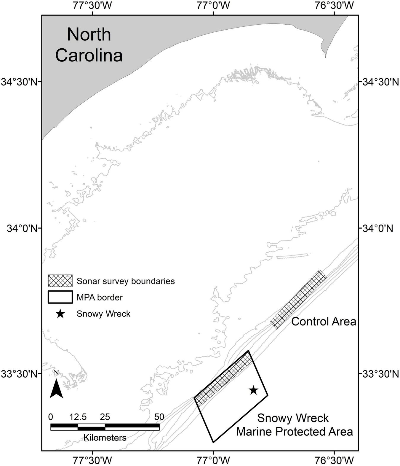
Map of the central North Carolina (United States) coastline. Checkered boxes delineate the survey extent within the Snowy Wreck Marine Protected Area and the control area for the present study and from Rudershausen et al. (2010). The Snowy Wreck location is indicated with a star. Gray contour lines represent 20, 40, 60, 80, 100, 120, 140, and 160 m isobaths.
Since the eight SEUSA deep-water MPAs were created, only two studies to our knowledge have investigated their effectiveness. Bacheler et al. (2016) used video transects to examine species richness, combined density of all exploited species, and density of one common exploited species (vermilion snapper; Rhomboplites aurorubens) inside five of the eight MPAs (including the SWMPA) for data collected through 2014. In addition, they used non-metric multidimensional scaling (NMDS) and analysis of similarity (ANOSIM) to compare fish communities inside versus outside MPAs. None of the analyses performed in Bacheler et al. (2016) indicated that the SEUSA MPA network was successful in increasing reef fish density or species richness. Most recently, Pickens et al. (2021) evaluated three of the MPAs (Northern South Carolina, Edisto, and North Florida MPAs) using video and trap catch information from 2011 to 2017 and reported no significant increases within MPAs relative to outside areas for any metric examined. Both Bacheler et al. (2016) and Pickens et al. (2021) concluded that while no positive MPA effects were found in their studies, further research was warranted.
Aware of the impending designation of the SWMPA, Rudershausen et al. (2010) collected hydroacoustic (fish biomass) and biological catch-per-unit-effort (CPUE) data in 2007–2009 in the soon-to-be-closed area as well as an adjacent area with the same general depth and habitat characteristics. In the present study, we re-analyzed and built upon the data collected by Rudershausen et al. (2010) and offer a third evaluation of the effects of a SEUSA MPA on rebuilding reef fish stocks. We build on the two prior studies by analyzing hydroacoustic data as well as species- and community-level data in a BACI design.
Materials and Methods
Study Site and Data Collection
We replicated the sampling methods of Rudershausen et al. (2010) and collected data inside the SWMPA along the continental shelf break in 47–150 m deep. Besides the shipwreck near the offshore edge of the area, the only known habitat for reef fish concentrations is along the inshore edge of the SWMPA (Rudershausen et al., 2010). Our sampling was therefore restricted to a 4.63 × 27.78 km rectangle inside the SWMPA as well as an adjacent area of equal dimensions that has never been closed to bottom fishing (hereafter: “control” or “control area”; Figure 1) that was also sampled in Rudershausen et al. (2010). Data collection trips from 2018 to 2020 were attended by at least one author of Rudershausen et al. (2010) and/or the collaborating boat captain from that study.
The null hypothesis in this study was that the SWMPA had no effect on overall biomass, abundance, individual size, and individual age of reef fishes. Within each area, we collected hydroacoustic backscatter and biological data to test this hypothesis. Hydroacoustic backscatter data were collected along a zig-zag track that connected alternating points along the inshore and offshore long edge of each rectangular area. Points along the edges of the areas through which we transected were spaced 4.63 km apart and specific paths were varied between trips so that we sampled new habitat each day. This followed the sampling protocol for the majority of the Rudershausen et al. (2010) data collection, though in 2007 the authors of that study conducted some transects in the SWMPA both parallel and perpendicular to the long edge of the area. For a given day of sampling, data were collected in either the SWMPA or the control area.
The modern study used an echosounder consisting of a Simrad ES60 transceiver outfitted with a single-beam transducer that operated at 38 kHz. We elected to use this gear because it was the exact unit used in Rudershausen et al. (2010). Acoustic data were collected from the R/V Cape Fear (20-m diesel-powered former fishing vessel) in 2018–2019 and from the R/V Regulator (8-m center-console vessel) in 2020. On both vessels, the transducer was mounted to the base of an aluminum pole and deployed off the port side so that the face of the transducer was approximately 0.5 m below the water surface. Boat speed ranged from three to five knots during acoustic data collection. The transceiver was connected to a laptop computer which was also connected to an on-board GPS plotter for positioning. During sampling, we noted the presence of any schools of on- or near-bottom (within 10 m of the seafloor) biomass (“acoustic events”) and recorded their GPS locations. Raw ES60 files were saved for subsequent processing. These methodologies are consistent with those of Rudershausen et al. (2010).
A subset of acoustic events were biologically sampled with hook-and-line. We determined ad hoc which events would be sampled with which gear based on a combination of the observed size of each acoustic event (to sample a range of fish group sizes) and their proximity to our vessel’s location (for logistical reasons). The choice of which acoustic events to sample was consistent between the SWMPA and control areas. Hook-and-line sampling gear consisted of conventional rods with electric reels and 59 kg braided line. Terminal tackle was a high-low bottom rig made of 68 kg monofilament line and two 8/0 J-style hooks and lead weight ranging from 0.68 to 1.36 kg. Hooks were baited with cut squid (Illex or Loligo sp.). Hook-and-line sampling usually took place within 24 h of acoustic data collection, though in one instance a hook-and-line trip took place 23 days after acoustic data collection.
When hook-and-line fishing, captains were permitted to keep vessels in gear (i.e., hover over events) or out of gear (i.e., drift) depending on sea conditions. Gear was deployed within ∼50 m of an acoustic event. Hook-and-line sampling was terminated when the boat drifted farther than ∼50 m from the event, whereupon the captain repositioned the boat. Hook-and-line sampling continued at an event until at least four drops of baited rigs had been conducted; a drop consisted of one vertical round-trip of a two-hook rig that was fully baited when deployed. Catch per unit effort (CPUE) was measured as fish-per-drop (regardless of species) for each baited two-hook rig. Caught reef fish were identified, measured (fork and total length; mm), and released. In 2019–2020, red porgy (Pagrus pagrus) were retained for aging.
Acoustic Data Processing
Acoustic data were processed using Echoview software (v. 10.0.275, Echoview Party Ltd.). We processed data that were collected during the present study (2018–2020) as well as raw acoustic data from the Rudershausen et al. (2010) study (collected in 2007–2009). For each data file, seafloor definitions were edited by one or two authors (BR and/or EE) and an impulse noise removal filter was applied to all files to reduce systematic non-biomass backscatter. Data were limited to backscatter stronger than -60 dB. For one analysis, we imposed a 100 m linear grid on each data file. Grid cells were bounded vertically by the seafloor and a line 10 m above it. This analysis yielded a total backscatter value for each 100 m × 10 m cell as the Nautical Area Scattering Coefficient (NASC; also called SA; units m2 nmi–2). The Echoview software calculated ensonified water volume accounting for beam spreading and scaled NASC values depending on depth. Additionally, we expected that habitat quality would be correlated with biomass; the continental shelf break inside the SWMPA and control area consists of stretches of low-slope unconsolidated sediment punctuated by high-relief drop-offs and ledges (Quattrini and Ross, 2006; Rudershausen et al., 2010). High vertical relief habitat is known to aggregate greater biomass of demersal fishes (Randall and Minns, 2000; Claisse et al., 2014), therefore we wished to include this metric in our statistical model. We generated an estimate of seafloor slope for each 100 m grid cell in our survey. Echoview exports included mean depth for each 100 m cell, so we estimated slope by generating a raster image for the inshore edge of the SWMPA and the control area using all mean depth observations from all acoustic sampling trips. Point values for mean depth were used to interpolate full coverage of each area using inverse distance weighting. Slope in degrees for each cell was then calculated using a 3 × 3 cell moving window of mean depth. Because this methodology relies on depth information from adjacent locations, we could not use it to estimate slope for some grid cells around the edge of each area. For these locations, we applied the slope from the nearest (linear distance) grid cell in which it was estimable. These analyses were conducted in R (R Core Team, 2021) and Esri ArcPro (v 2.7).
For a separate analysis, individual acoustic events (aggregations of fish) were defined and their acoustic backscatter was measured (again in terms of NASC). Only acoustic events that were sampled biologically in our study or during Rudershausen et al. (2010) were measured for this second analysis. The definition of what was considered a fish aggregation, determined by a single author (EE), was consistent across data files (and thus between areas and time periods), and made no assumptions about species composition. In general, fish aggregations were delineated by examining the echogram for clear areas of higher density; when several areas of higher density were adjacent to one another, they were usually considered distinct aggregations (depending on their size and spatial distribution).
Hurdle Model of Hydroacoustic Data
We fitted a series of lognormal hurdle models in a Bayesian framework to the 100 m grid cell hydroacoustic data using the R package “brms” (Bürkner, 2017). The first stage of the hurdle model estimated the probability of a given cell containing zero biomass and the second stage estimated the distribution of biomass given that it was non-zero. We fitted a range of candidate models to the data. The full model included Area (SWMPA or control) and Period (before or after) as main effects as well as their two-way interaction. In a BACI design such as our own, an Area:Period interaction tests for an MPA effect; if the directionality and/or magnitude of change through time differs between the two areas, this suggests that designation of the MPA (or “impact”) is the cause. In addition to these main effects, we included a fixed effect for seafloor slope (Slope; continuous), a fixed effect for season (Season; factor; winter, spring, summer, and fall), and a random effect for trip (Trip; intended to account for stochasticity in environmental conditions that we were unable to measure). We considered including seafloor depth as a variable in these models, however, ad hoc investigations revealed that depth and slope were highly correlated. This was unsurprising considering the most extreme drop-off of the continental shelf tends to occur around the same depth regardless of latitude. The correlation between these two variables was non-linear (Supplementary Figure 1), and a generalized additive model (GAM; R package “mgcv”; Wood, 2011) revealed that the relationship was highly significant (Supplementary Figure 2; edf = 8.5; p < 0.001). We therefore excluded depth as a predictor variable in all models.
The full model was specified as:
Where hu_β0 through hu_β5 and β0 through β5 were given a prior of Normal(0,10), hu_αj and αj were given a prior of Normal(0, hu_σTrip) and Normal(0, σTrip) respectively, and hu_σTrip and σTrip were given a prior of HalfCauchy(10). These priors were generally uninformative but may have weakly constrained the parameter estimates to exclude outlying observations. In this model, Yi is the amount of biomass (NASC) per 100-m grid cell in the sonar survey, β terms describe coefficients for each variable, αj is a random intercept for trip j, and σj is a random standard deviation for the intercept term for trip j. Other candidate models included different combinations of these variables, starting with the most basic model (intercept only) and working up to the full model. Candidate models were examined only if they were deemed biologically plausible and no three-way interaction terms were included in any model (Table 1). All models used the same effects for both model stages, as we assume that a covariate that is associated with high encounter probability will also likely be associated with high biomass (Thorson, 2018). Each model was fitted assuming a lognormal distribution and using four sampling chains, each with 10,000 iterations, a burn-in period of 1,000 iterations, and thinning of every third sample. We examined model output, including R-hat and effective sample size, to ensure convergence. We used Widely Applicable Information Criterion (WAIC) to compare our candidate models and select the best model; WAIC is useful for comparing complex Bayesian models and often outperforms other metrics such as AIC or DIC (Watanabe and Opper, 2010; Gelman et al., 2014). Meaningfulness of partial regression coefficients was evaluated by examining 95% credible intervals and checking whether they contained zero.
TABLE 1
| Model variables | WAIC | ΔWAIC |
| ∼ Period + Slope + Season + Trip | 52,211.2 | 0 |
| ∼ Area + Period + Slope + Trip | 52,212.4 | 0.2 |
| ∼ Area * Period + Slope + Trip | 52,212.7 | 0.5 |
| ∼ Area * Period + Slope + Season + Trip | 52,212.7 | 0.5 |
| ∼ Slope + Trip | 52,212.7 | 0.5 |
| ∼ Slope + Season + Trip | 52,212.8 | 0.6 |
| ∼ Area + Slope + Season + Trip | 52,212.8 | 0.6 |
| ∼ Period + Slope + Trip | 52,213.0 | 1.8 |
| ∼ Area + Slope + Trip | 52,213.4 | 2.6 |
| ∼ 1 | 56,263.6 | 4,052.4 |
Candidate models examined for their fit to the data consisting of NASC, the amount of acoustic backscatter (i.e., fish biomass) in each 100 m grid cell in our sonar survey in marine protected area (MPA) and control areas and periods (Before and After closure).
An asterisk (*) between two terms indicates that both effects were examined individually as was the two-way interaction between them. The model with no variables (i.e., “1”) is the intercept-only model, included for comparison. Where it was included, Trip was modeled as a random effect. Widely Applicable Information Criterion (WAIC) is presented for each model, and the model with the lowest WAIC is considered to be the best.
Catch per Unit Effort Analyses
We also fitted hurdle models to the data consisting of Catch Per Unit Effort (CPUE) at sites that were biologically sampled. In this procedure, the first stage of the hurdle model estimated the probability of a given site producing zero CPUE (no fish caught) and the second stage estimated the distribution of CPUE given that it was non-zero. We again fitted a range of candidate models to the data, beginning with an intercept only model and working up to various combinations of the main effects (Area and Period) and the Area:Period interaction along with a fixed effect of biomass (NASC) calculated at each individual site (Table 2). Finally, we included a random effect of Trip in some candidate models, intended to account for among-day variability in sea conditions and fish catchability.
TABLE 2
| Model variables | All species |
Assessed species only |
||
| WAIC | ΔWAIC | WAIC | ΔWAIC | |
| ∼ Area + Trip | 228.6 | 0 | 213.6 | 1.7 |
| ∼ Period + Trip | 228.8 | 0.2 | 211.9 | 0 |
| ∼ Area + Period + Trip | 230.4 | 1.8 | 214.9 | 3 |
| ∼ Area + Period | 231.9 | 3.3 | 218.6 | 6.7 |
| ∼ Area + Period + NASC + Trip | 232.4 | 3.8 | 218.0 | 6.1 |
| ∼ Area * Period + Trip | 232.8 | 4.2 | 217.4 | 5.5 |
| ∼ Area + Period + NASC | 234.4 | 5.8 | 221.8 | 9.9 |
| ∼ Area | 234.8 | 6.2 | 221.7 | 9.8 |
| ∼ Area * Period + NASC + Trip | 235.8 | 7.2 | 220.3 | 8.4 |
| ∼ 1 | 240.2 | 11.6 | 220.1 | 8.2 |
Candidate models examined for their fit to the data consisting of catch-per-unit-effort (CPUE) for all species and assessed species only at each site sampled with hook-and-line in both areas (Snowy Wreck Marine Protected Area or Control) and periods (Before and After).
NASC is the amount of acoustic backscatter (i.e., fish biomass) at each site. An asterisk (*) between two terms indicates that both effects were examined individually as was the two-way interaction between them. Where it was included, Trip was modeled as a random effect. The model with no variables (i.e., “1”) is the intercept-only model, included for comparison. Widely Applicable Information Criterion (WAIC) is presented for each model, and the model with the lowest WAIC is considered to be the best.
The full model was specified as:
All models used the same effects for both model stages, and all models were fitted assuming a lognormal distribution using four sampling chains, each with 10,000 iterations, a burn-in period of 1,000 iterations, and thinning of every third sample. Prior distributions, model evaluation, and parameter evaluation occurred as above. We replicated this modeling procedure for a subset of CPUE data consisting of only species that have formal stock assessments in this region, which is an indication of their economic importance and a reasonable proxy for how heavily they have been targeted in recent decades. For this analysis, we included CPUE data for only blueline tilefish (Caulolatilus microps), gag (Mycteroperca microlepis), gray triggerfish (Balistes capriscus), greater amberjack (Seriola dumerili), red grouper (E. morio), red porgy (Pagrus pagrus), scamp (M. phenax), snowy grouper (H. niveatus), and vermilion snapper. Finally, we performed a qualitative investigation of overall CPUE trends in the four crosses of Area and Period for CPUE of all reef fish and CPUE of assessed species only. This analysis was conducted with per-trip CPUE.
Multivariate Analysis of Community Composition
We examined reef fish community composition in both periods and areas using non-metric multidimensional scaling (NMDS) and analysis of similarities (ANOSIM). NMDS and ANOSIM have been used to characterize fish communities in impacted areas as compared to control sites (Shepherd et al., 1992; Bacheler et al., 2016). We treated each area/period cross as an independent community of reef fish. Given that gear was standardized between time periods, we assumed that changes in catch reflected changes in the community rather than an effect of sampling. Our sampling unit was each trip during which reef fish were caught; we could have divided the data to the site level, but many sites produced zero catch which would require their exclusion from community analyses. We binned reef fish into six groups: groupers (Serranidae), jacks (Carangidae), porgies (Sparidae), snappers (Lutjanidae), tilefish (Malacanthidae), and triggerfish (Balistidae) (Table 3). Observations of species that did not fit into these groups were rare (<5% of all catch) and were therefore excluded from the community analyses. Catch data were standardized by effort (number of drops) for a given trip, yielding a CPUE value for each trip and species group; relative rather than absolute values are required for NMDS when sampling effort is variable (Clarke, 1993). CPUE data were fourth-root transformed to down-weight the dominance of highly abundant species groups (Clarke and Warwick, 2001). Relationships between crosses of area and period were visualized by plotting NMDS results based on zero-adjusted Bray-Curtis similarity; this adjustment controls for erratic behavior that sometimes occurs for zero-rich data (Clarke et al., 2006). We conducted a one-way ANOSIM using the same zero-adjusted Bray-Curtis similarities as in the NMDS analysis. The ANOSIM was used to calculate an R statistic and differences between the four communities were evaluated for significance at α = 0.05. Multivariate analyses were performed in the R package “vegan” (Oksanen et al., 2020).
TABLE 3
| Species | Community grouping | MPA-before | Control-before | MPA-after | Control-after |
| Almaco jack Seriola rivoliana | Jacks | 0.005 | 0 | 0.036 | 0.014 |
| Atlantic creolefish Paranthias furcifer | – | 0.003 | 0 | 0.001 | 0.002 |
| Blackfin snapper Lutjanus buccanella | Snappers | 0 | 0 | 0.006 | 0 |
| Blueline tilefish Caulolatilus microps | Tilefish | 0.005 | 0 | 0.011 | 0 |
| Coney Cephalopholis fulva | Groupers | 0 | 0.020 | 0.001 | 0 |
| Gag Mycteroperca microlepis | Groupers | 0.003 | 0 | 0.001 | 0 |
| Goldface tilefish Caulolatilus chrysops | Tilefish | 0 | 0 | 0.003 | 0 |
| Gray triggerfish Balistes capriscus | Triggerfish | 0.005 | 0 | 0.017 | 0.009 |
| Graysby Cephalopholis cruentata | Groupers | 0.011 | 0 | 0 | 0 |
| Greater amberjack Seriola dumerili | Jacks | 0.008 | 0 | 0.006 | 0 |
| Hogfish Lachnolaimus maximus | – | 0.003 | 0 | 0 | 0 |
| Hybrid snapper Lutjanus sp. | Snappers | 0 | 0 | 0.001 | 0 |
| Jolthead porgy Calamus bajonado | Porgies | 0.003 | 0.010 | 0 | 0.007 |
| Knobbed porgy Calamus nodosus | Porgies | 0.016 | 0.070 | 0.010 | 0.019 |
| Lesser amberjack Seriola fasciata | Jacks | 0.003 | 0 | 0 | 0 |
| Marbled grouper Dermatolepis inermis | Groupers | 0 | 0 | 0.001 | 0 |
| Moray Gymnothorax sp. | – | 0 | 0 | 0.001 | 0 |
| Red cornetfish Fistularia petimba | – | 0.003 | 0 | 0 | 0 |
| Red grouper Epinephelus morio | Groupers | 0.016 | 0.020 | 0.003 | 0 |
| Red porgy Pagrus | Porgies | 0.109 | 0.220 | 0.166 | 0.074 |
| Rock hind Epinephelus adscensionis | Groupers | 0.005 | 0 | 0 | 0 |
| Sand tilefish Malacanthus plumieri | Tilefish | 0 | 0 | 0.005 | 0.037 |
| Scamp Mycteroperca phenax | Groupers | 0.033 | 0 | 0.014 | 0.007 |
| Short bigeye Pristigenys alta | – | 0.005 | 0 | 0.004 | 0 |
| Silk snapper Lutjanus vivanus | Snappers | 0 | 0 | 0.032 | 0.058 |
| Snowy grouper Hyporthodus niveatus | Groupers | 0.057 | 0.030 | 0.060 | 0.009 |
| Speckled hind Epinephelus drummondhayi | Groupers | 0.022 | 0 | 0.006 | 0 |
| Spinycheek scorpionfish Neomerinthe hemingwayi | – | 0.003 | 0 | 0.001 | 0 |
| Squirrelfish Holocentrus adscensionis | – | 0 | 0 | 0.001 | 0.002 |
| Tattler Serranus phoebe | – | 0.005 | 0.010 | 0.010 | 0.007 |
| Tomtate Haemulon aurolineatum | – | 0.022 | 0 | 0 | 0 |
| Vermilion snapper Rhomboplites aurorubens | Snappers | 0.003 | 0 | 0.068 | 0.035 |
| White grunt Haemulon plumierii | – | 0 | 0 | 0.001 | 0 |
| Whitebone porgy Calamus leucosteus | Porgies | 0 | 0 | 0.004 | 0 |
| Whitespotted soapfish Rypticus maculatus | – | 0 | 0 | 0 | 0.002 |
| Yellowmouth grouper Mycteroperca interstitialis | Groupers | 0 | 0 | 0.005 | 0 |
All reef fish species encountered in the present study and in Rudershausen et al. (2010).
Catch per unit effort (CPUE) values are fish/drop. MPA refers to the Snowy Wreck Marine Protected Area, and Control refers to an adjacent area that is open to bottom fishing. Community grouping is the taxonomic group in which each species was included for multivariate analyses.
Red Porgy Age Analyses
We conducted single-species analyses with red porgy for several reasons. First, they were the most frequently caught species in both areas and time periods; other species lacked appropriate sample sizes in one or more areas or periods (see “Results”). Moreover, red porgy have fairly narrow home ranges relative to the size of the SWMPA; short term ranges are generally ∼0.5 km2 (Afonso et al., 2009) while the entire SWMPA is >500 km2. Red porgy reach reproductive maturity quickly, with most spawning by age 2 or 3 (Manooch and Huntsman, 1977; Wyanski et al., 2019). Given the size and age of the SWMPA relative to these biological characteristics of red porgy, this species represented an ideal candidate for testing a monospecific MPA effect. Moreover, for similar reasons, Pickens et al. (2021) conducted single-species analyses for red porgy caught in three of the other SEUSA MPAs; by singling out this species, we added to their analysis of how SEUSA MPAs are affecting biological metrics of red porgy.
For red porgy collected in 2019–2020, fish were weighed (whole weight; g) and sagittal otoliths were removed. Otoliths were processed and analyzed at the NOAA Fisheries Laboratory in Beaufort, North Carolina, using the methods described by Burton et al. (2017). Calendar ages were assigned to each specimen based on the number of opaque annuli and the month of capture (J. Potts, NOAA Fisheries, personal communication). In addition to red porgy collected by our survey, we obtained age information for red porgy caught by the Southeast Reef Fish Survey (SERFS) in the SWMPA and the surrounding region of Onslow Bay, NC, including the control area, from 2015 to 2019 (T. Smart, SC DNR, personal communication). SERFS data were only available through 2019, so red porgy encountered in 2020 for both inside control and outside SWMPA were all from our collections in the control area. Sample sizes in the SWMPA prior to 2015 were insufficient for inclusion. Similarly, no red porgy ages were available from Rudershausen et al. (2010), which precluded a BACI framework for this analysis. Red porgy collected in the present study were collected with hook-and-line and chevron traps (B. Runde, unpublished data); red porgy from SERFS were collected with chevron traps and short bottom longlines. We assumed that the selectivity of these gears is equivalent because a recent stock assessment of this species used logistic selectivity curves for hook-based gear as well as traps, and both curves used age 6 as the youngest age of full recruitment to the gear (SEDAR, 2020). We examined age frequencies of red porgy by area (SWMPA or control) and year (2015–2020). We calculated mean age by area and year and compared yearly means using a Wilcoxon rank-sum test. Significance was assessed at α = 0.05 with a Bonferroni correction applied such that α = 0.008. In addition to mean age, we compared yearly age diversity between the SWMPA and control sites using the Shannon diversity index. Age diversity is an important metric of fish stock health, with higher diversity implying greater health (Marteinsdottir and Thorarinsson, 1998). Diversity values were calculated using the R package “vegan” (Oksanen et al., 2020).
Red Porgy Size Distributions
We compared size (TL, mm) distributions of red porgy caught by the authors of Rudershausen et al. (2010) with those caught in 2018–2020 in both areas. To augment our dataset in the latter period, we obtained length information for red porgy caught by SERFS in these two areas (T. Smart, personal communication). As in the age analysis, we assume selectivity of gears used in these surveys was equivalent for red porgy. For the size analysis, we did not use red porgy data from elsewhere in the region; analyses were restricted to individuals that were caught in either the SWMPA or the control area. We did not expand our dataset to include fish from outside the control area because data were not available from SERFS in the “before” period. We used Bayesian linear model to compare the four size distributions (TL, centered) and tested for the effect of Area, Period, and their interaction. Meaningfulness was evaluated based on whether or not the credible intervals contained zero.
Results
Summary of Field Work and Resultant Data We made five trips each to the SWMPA and the control area for sonar data collection between 2018 and 2020. In the SWMPA, we identified 163 aggregations of biomass in total, of which 41 were fished with 250 total hook-and-line drops. In the control area, we identified 207 total aggregations of biomass of which 72 were fished with 382 total hook-and-line drops. We caught at least one individual of 29 fish species with hook-and-line. In the SWMPA, species-specific CPUE ranged from 0.001 to 0.166 fish per drop. In the control area, CPUE values ranged from 0.002 to 0.074; many of these CPUE values were similar to Rudershausen et al. (2010; Table 3).
Hurdle Model of Hydroacoustic Data
Across both areas and periods, sonar data collection resulted in 10,951 grid cells of 100 m length. The distribution of non-zero density (NASC) observations in these cells was approximately lognormal (Figure 2). The best model (lowest WAIC) was Period + Slope + Season + Trip (Table 1). There were several additional models that were competitive in terms of WAIC; each of these models contained Slope and Trip. Results from the best model indicated meaningful effects of Slope in both stages of the model; cells with higher slope were less likely to contain zero biomass, and given non-zero biomass, cells with higher slope had higher biomass (Table 4 and Supplementary Figure 3). In this model, the only other variable whose credible interval for its partial regression coefficient that did not include zero was Period, for which the before period had less biomass than the after period (Supplementary Figure 4). We also investigated results from the full model given that it was nearly equivalent to the best model in terms of WAIC (ΔWAIC = 0.5, Table 1). The only variable whose partial regression coefficient did not include zero in either stage of this model was Slope (Table 5).
FIGURE 2
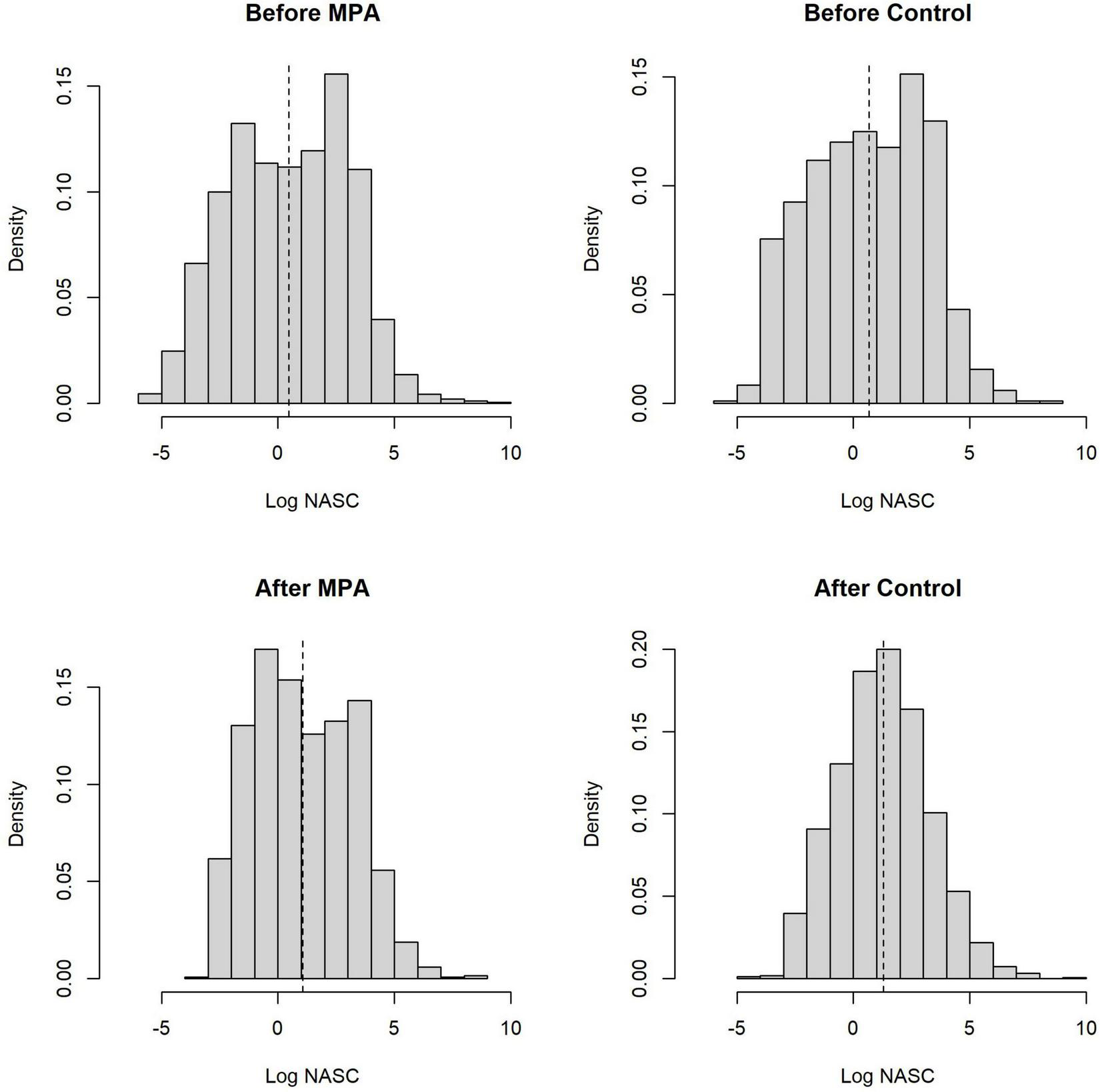
Distributions of the natural logarithm of all non-zero biomass observations from our sonar analysis, broken down by Area and Period. Each observation represents the total biomass volume (NASC) per 100 m grid cell. Vertical dashed lines are the mean of the distributions.
TABLE 4
| Variable | Estimate | Est. error | 2.5% CI | 97.5% CI | Rhat | ESS |
| Trip Sd(Intercept) | 0.60 | 0.13 | 0.41 | 0.91 | 1.00 | 10, 733 |
| Intercept | 1.16 | 0.33 | 0.49 | 1.82 | 1.00 | 17, 228 |
| PeriodBefore | –0.62 | 0.29 | –1.17 | –0.03 | 1.00 | 17, 666 |
| Slope | 0.45 | 0.03 | 0.39 | 0.51 | 1.00 | 15, 130 |
| SeasonSpring | –0.46 | 0.47 | –1.39 | 0.46 | 1.00 | 17, 686 |
| SeasonSummer | –0.56 | 0.36 | –1.27 | 0.16 | 1.00 | 16, 573 |
| SeasonWinter | –0.46 | 0.43 | –1.31 | 0.37 | 1.00 | 17, 234 |
| Trip Sd(Hu_Intercept) | 1.32 | 0.25 | 0.93 | 1.90 | 1.00 | 10, 614 |
| Hu_Intercept | –0.46 | 0.70 | –1.88 | 0.89 | 1.00 | 17, 026 |
| Hu_PeriodBefore | –1.18 | 0.61 | –2.36 | 0.03 | 1.00 | 16, 670 |
| Hu_slope | –0.35 | 0.03 | –0.41 | –0.29 | 1.00 | 15, 050 |
| Hu_SeasonSpring | 1.03 | 0.99 | –0.91 | 2.99 | 1.00 | 16, 492 |
| Hu_SeasonSummer | 0.77 | 0.77 | –0.69 | 2.31 | 1.00 | 16, 715 |
| Hu_SeasonWinter | 0.98 | 0.92 | –0.85 | 2.79 | 1.00 | 16, 820 |
Results from the biomass hurdle model with the lowest Widely Applicable Information Criterion (WAIC): Period + Slope + Season + Trip.
Variables containing “hu” pertain to the first stage of the hurdle model. ESS refers to the effective sample size.
TABLE 5
| Variable | Estimate | Est. error | 2.5% CI | 97.5% CI | Rhat | ESS |
| Trip Sd(Intercept) | 0.61 | 0.14 | 0.41 | 0.95 | 1.00 | 9, 910 |
| Intercept | 1.36 | 0.41 | 0.55 | 2.17 | 1.00 | 11, 566 |
| PeriodBefore | –0.38 | 0.53 | –1.42 | 0.70 | 1.00 | 10, 935 |
| AreaMPA | –0.28 | 0.43 | –1.14 | 0.59 | 1.00 | 11, 666 |
| SeasonSpring | –0.66 | 0.53 | –1.71 | 0.35 | 1.00 | 11, 363 |
| SeasonSummer | –0.55 | 0.36 | –1.29 | 0.13 | 1.00 | 11, 201 |
| SeasonWinter | –0.72 | 0.50 | –1.70 | 0.30 | 1.00 | 11, 247 |
| Slope | 0.45 | 0.03 | 0.39 | 0.51 | 1.00 | 11, 194 |
| AreaMPA:PeriodBefore | –0.21 | 0.64 | –1.48 | 1.10 | 1.00 | 11, 528 |
| Trip Sd(Hu_Intercept) | 1.42 | 0.29 | 0.98 | 2.10 | 1.00 | 10, 466 |
| Hu_Intercept | –0.42 | 0.91 | –2.20 | 1.43 | 1.00 | 11, 547 |
| Hu_PeriodBefore | –1.24 | 1.17 | –3.54 | 1.00 | 1.00 | 10, 980 |
| Hu_AreaMPA | –0.06 | 0.96 | –1.90 | 1.86 | 1.00 | 10, 679 |
| Hu_SeasonSpring | 1.04 | 1.15 | –1.30 | 3.31 | 1.00 | 11, 568 |
| Hu_SeasonSummer | 0.77 | 0.80 | –0.85 | 2.38 | 1.00 | 11, 139 |
| Hu_SeasonWinter | 0.98 | 1.13 | –1.29 | 3.19 | 1.00 | 11, 350 |
| Hu_Slope | –0.35 | 0.03 | –0.41 | –0.29 | 1.00 | 10, 857 |
| Hu_AreaMPA:PeriodBefore | 0.10 | 1.44 | –2.65 | 3.03 | 1.00 | 11, 375 |
Results from the biomass model containing the full suite of predictor variables, which was competitive with the best model in terms of WAIC.
Variables containing “hu” pertain to the first stage of the hurdle model. ESS refers to the effective sample size.
Catch Per Unit Effort Analyses
The best model for predicting CPUE of all reef species was Area + Trip followed by a model with Period + Trip (Table 2). For assessed reef species CPUE, the same two models were best, though in reverse order. In neither of the top two models did the 95% credible intervals for any predictor variable contain zero in either stage of the model, regardless of whether all reef species CPUE or assessed species CPUE was used (Tables 6, 7). Other models were not competitive.
TABLE 6
| CPUE species | Variable | Estimate | Est. error | 2.5% CI | 97.5% CI | Rhat | ESS |
| All | Trip Sd(Intercept) | 0.28 | 0.11 | 0.09 | 0.52 | 1.00 | 7289 |
| Intercept | –1.21 | 0.14 | –1.49 | –0.94 | 1.00 | 10956 | |
| AreaMPA | 0.30 | 0.19 | –0.09 | 0.66 | 1.00 | 11117 | |
| Trip Sd(Hu_Intercept) | 0.30 | 0.22 | 0.01 | 0.83 | 1.00 | 9650 | |
| Hu_Intercept | –0.32 | 0.27 | –0.84 | 0.18 | 1.00 | 10880 | |
| Hu_AreaMPA | 0.42 | 0.36 | –0.27 | 1.13 | 1.00 | 11557 | |
| Assessed | Trip Sd(Intercept) | 0.47 | 0.16 | 0.17 | 0.82 | 1.00 | 6337 |
| Intercept | –1.31 | 0.22 | –1.74 | –0.88 | 1.00 | 10569 | |
| AreaMPA | 0.09 | 0.29 | –0.49 | 0.65 | 1.00 | 11045 | |
| Trip Sd(Hu_Intercept) | 0.28 | 0.22 | 0.01 | 0.82 | 1.00 | 9280 | |
| Hu_Intercept | 0.71 | 0.27 | 0.19 | 1.23 | 1.00 | 11956 | |
| Hu_AreaMPA | –0.44 | 0.37 | –1.16 | 0.28 | 1.00 | 12584 |
Results from the Area + Trip hurdle model for predicting reef fish CPUE.
Model results are shown for a model run with CPUE of all reef species and a separate run for CPUE of assessed reef species only. Variables from the first stage of the hurdle model begin with “Hu,” and coefficient values are provided in untransformed logit terms.
TABLE 7
| CPUE species | Variable | Estimate | Est. error | 2.5% CI | 97.5% CI | Rhat | ESS |
| All | Trip Sd(Intercept) | 0.33 | 0.10 | 0.15 | 0.56 | 1.00 | 9, 033 |
| Intercept | –0.99 | 0.13 | –1.26 | –0.73 | 1.00 | 11, 087 | |
| PeriodBefore | –0.15 | 0.20 | –0.53 | 0.25 | 1.00 | 11, 300 | |
| Trip Sd(Hu_Intercept) | 0.28 | 0.21 | 0.01 | 0.78 | 1.00 | 10, 703 | |
| Hu_Intercept | –0.25 | 0.23 | –0.69 | 0.21 | 1.00 | 11, 330 | |
| Hu_PeriodBefore | 0.38 | 0.35 | –0.34 | 1.08 | 1.00 | 11, 151 | |
| Assessed | Trip Sd(Intercept) | 0.43 | 0.17 | 0.11 | 0.79 | 1.00 | 6, 485 |
| Intercept | –1.09 | 0.19 | –1.48 | –0.73 | 1.00 | 10, 594 | |
| PeriodBefore | –0.34 | 0.27 | –0.88 | 0.20 | 1.00 | 11, 022 | |
| Trip Sd(Hu_Intercept) | 0.28 | 0.21 | 0.01 | 0.78 | 1.00 | 9, 659 | |
| Hu_Intercept | 0.70 | 0.24 | 0.24 | 1.18 | 1.00 | 11, 011 | |
| Hu_PeriodBefore | –0.57 | 0.37 | –1.31 | 0.16 | 1.00 | 12, 526 |
Results from the Period + Trip hurdle model for predicting reef fish CPUE.
Model results are shown for a model run with CPUE of all reef species and a separate run for CPUE of assessed reef species only. Variables from the first stage of the hurdle model begin with “Hu,” and coefficient values are provided in untransformed logit terms.
Qualitative investigations of CPUE revealed interesting trends. When all reef species CPUE was used, a positive temporal trend was evident in the Control area (53.6% increase) but not the SWMPA (9.9% decrease). When only assessed species CPUE was used, the trend for the Control was negative (13.0% decrease) and a positive trend (28.6% increase) for the SWMPA emerged (Figure 3). Overall combined CPUE values (i.e., n fish/n drops across all trips) for assessed species in the SWMPA increased from 0.027 to 0.039 (47.3% increase) from the before to the after period. In the Control area, the same metric decreased from 0.030 to 0.015 (50.4% decrease).
FIGURE 3
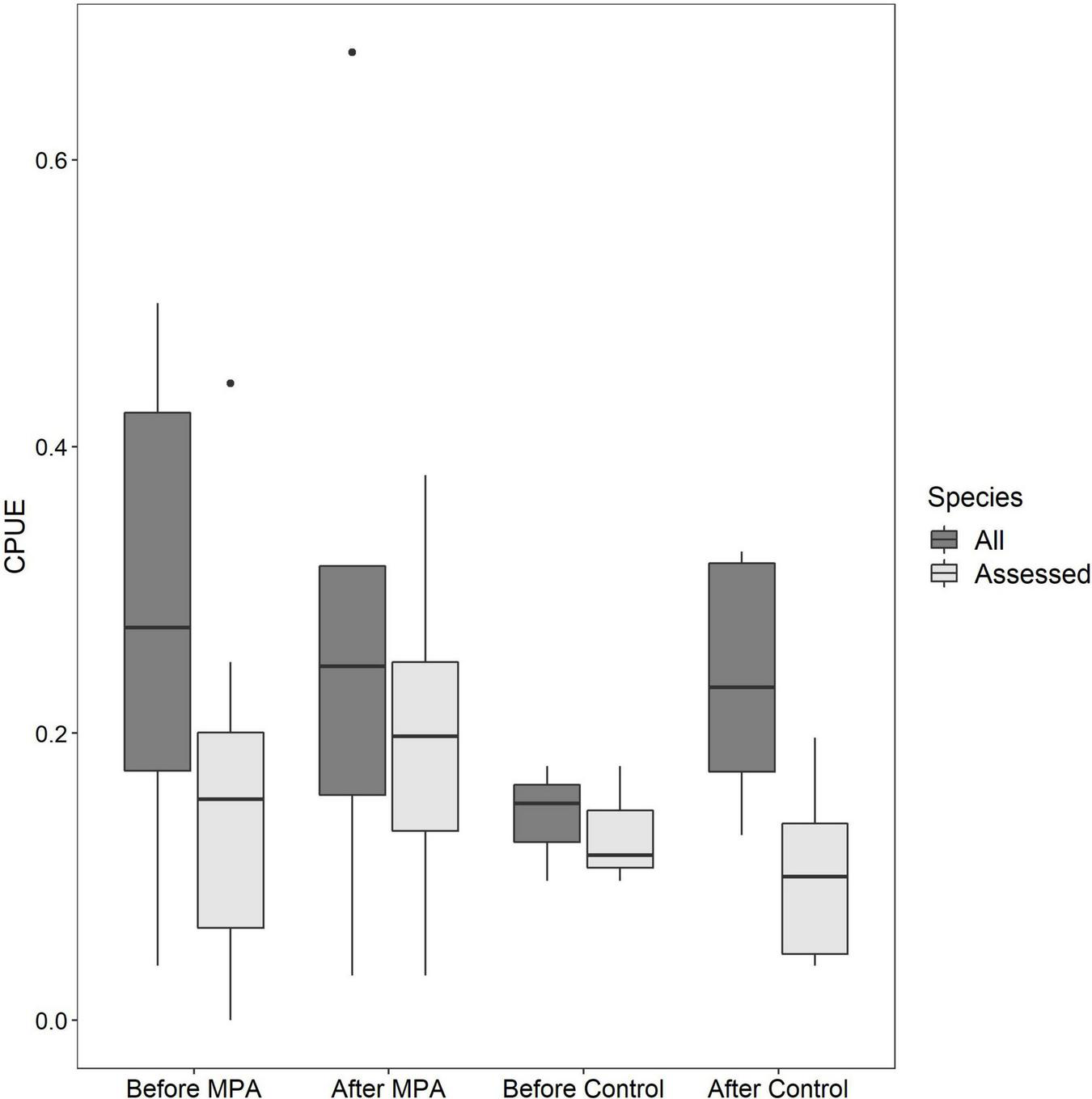
Boxplots of per-trip catch per unit effort among the four crosses of Area and Period using all reef fish catch-per-unit-effort (CPUE) (dark boxes) and CPUE for only assessed species (light boxes).
Multivariate Analysis of Community Composition
The four Area/Period combinations each had distinct communities. NMDS indicated four groupings with minimal overlap and had an estimated stress value of 0.131, indicating a fair or good fit (Figure 4). NMDS results suggested changes in occurrence from more groupers to more snappers and tilefish in both areas. From the ANOSIM procedure, the R statistic was 0.454 with an associated p value of 0.001, indicating significant separation among the four communities. The results from these multivariate analyses indicate that fish communities have changed without respect to the area (MPA vs. control).
FIGURE 4
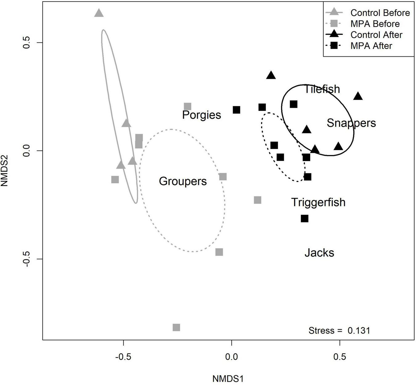
Results of non-metric multidimensional scaling (NMDS) comparing reef fish communities in the two areas (Snowy Wreck Marine Protected Area and control) and time periods (before and after). A stress value of 0.131 indicates a fair to good fit.
Red Porgy Age Analyses
Annual sample sizes for red porgy ages from 2015 to 2020 ranged from 14 to 67 inside the SWMPA and from 8 to 73 inside the control area. For all red porgy from outside the SWMPA, yearly sample sizes ranged from 386 to 546. Mean annual ages ranged from 4.9 to 7.1 inside the SWMPA and from 4.8 to 5.3 in the control area, and were higher in the SWMPA for each of the 6 years examined. Wilcoxon rank sum tests found that ages were significantly higher in the SWMPA than the control in 2016 and 2018 (Figure 5). Age diversity values ranged from 1.7 to 2.0 inside the SWMPA and from 0.9 to 2.0 in the control. Diversity values were higher inside the SWMPA for five out of 6 years examined (Figure 5).
FIGURE 5
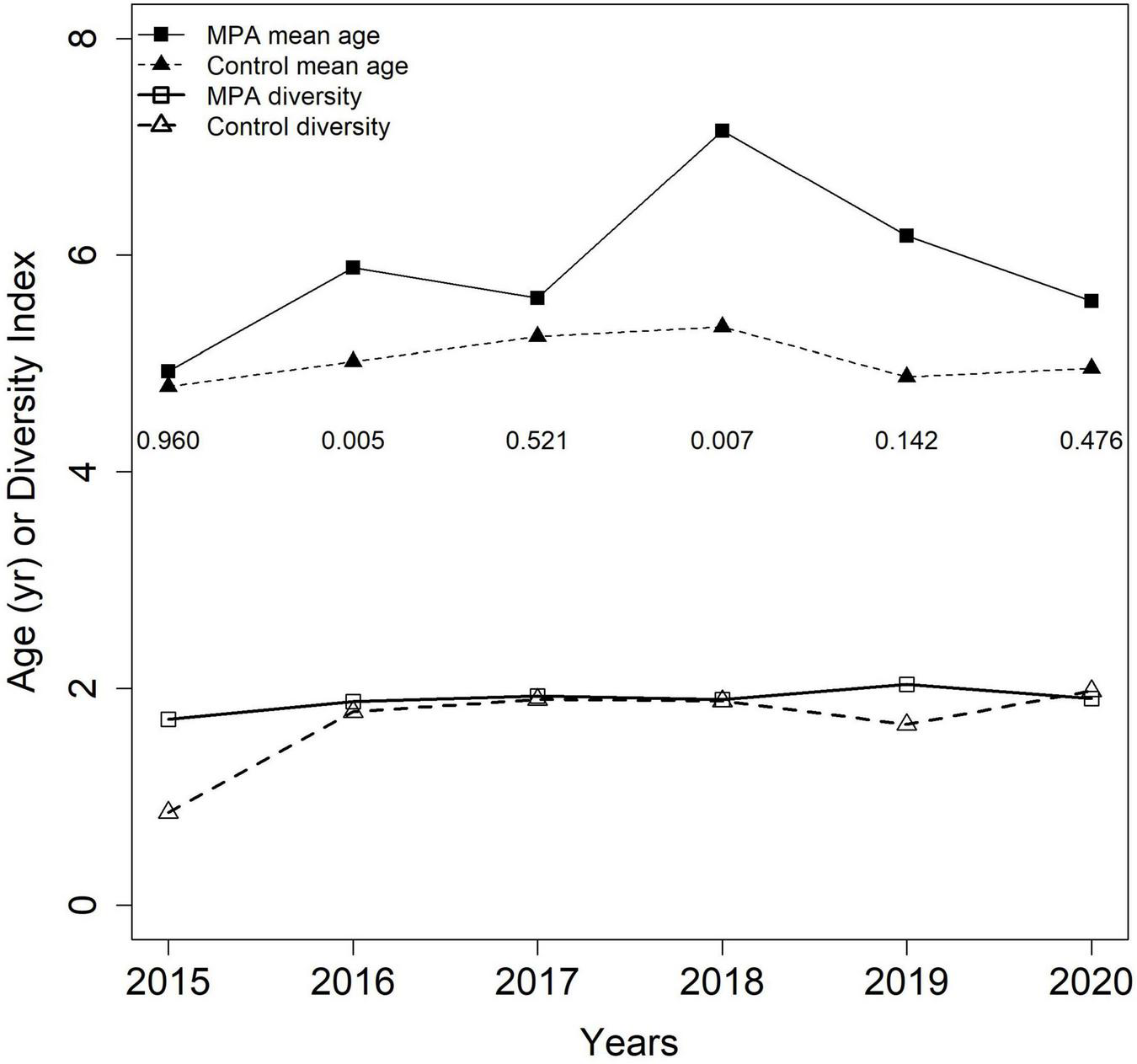
Mean age and Shannon age diversity for red porgy caught in the Snowy Wreck Marine Protected Area and adjacent control area from 2015 to 2020 by our survey or the Southeast Reef Fish Survey. Numbers displayed below mean ages are p-values resulting from annual between-area Wilcoxon rank sum tests.
Red Porgy Size Distributions
Rudershausen et al. (2010) collected lengths for 26 red porgy in the control area and 41 red porgy in the SWMPA in 2007–2009. Between data from the present study and SERFS data, lengths were available for 89 red porgy in the control area and 181 red porgy in the SWMPA from 2018 to 2020. Size distributions showed an increase in red porgy total lengths in the SWMPA from the before to the after period but no shift was evident in the control area (Figure 6). Our Bayesian linear model revealed that the Area∗Period interaction was meaningful, as its credible interval did not overlap zero. This result indicates a positive effect of MPA designation on the size structure of red porgy inside the SWMPA.
FIGURE 6
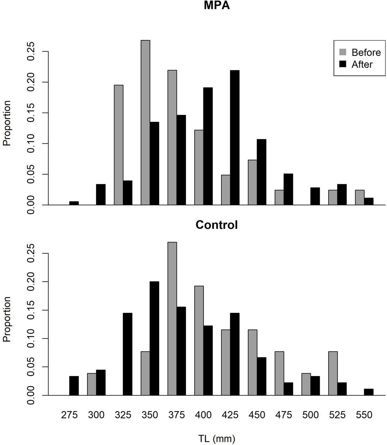
Size (total length) distributions for red porgy caught in the Snowy Wreck Marine Protected Area (SWMPA) and the adjacent control area in the before period (2007–2009) by Rudershausen et al. (2010) and in the present study (after; 2018–2020).
Discussion
Using MPAs to protect, conserve, or rebuild fish populations has often led to detectable increases in biological metrics (Lester et al., 2009). However, the strength of the effect (and its detectability) depends on the context: characteristics of the protected species and the MPA, as well as study design, can all influence the detection of MPA effectiveness (Edgar et al., 2014). Our results indicate that the SWMPA is not helping to increase the abundance or biomass of rare and threatened species that it was intended to protect (e.g., speckled hind). Whether the other deepwater MPAs in this region are now providing this service is an important topic of future research; such research would help better determine whether deepwater MPAs are the viable management tool and sanctuary for these imperiled species that federal fishery managers envisioned (SAFMC, 2010). Our results indicate some positive effects of the Snowy Wreck Marine Protected Area on metrics for reef fish, but these findings were restricted to CPUE trends and monospecific (red porgy) analyses and did not apply to our analysis of hydroacoustic data. These equivocal findings corroborate prior studies of the MPAs in this region (Bacheler et al., 2016; Pickens et al., 2021).
Models fitted to hydroacoustic data did not reveal an MPA effect. It is possible that there has truly been no effect of the SWMPA on biomass, or that our survey was not comprehensive enough to detect it. However, other possibilities exist as well. The measures of acoustic backscatter cannot be attributed to species or size groups and therefore a mix of target and non-target species are likely contributing to the magnitude of backscatter in both the SWMPA and control. Therefore, overall fish biomass (or density) may not have increased in the SWMPA but it may now consist of older and larger individuals; this hypothesis is supported by the red porgy size analysis discussed below. It is unsurprising that Slope was a significant predictor of biomass in our hurdle models, since greater vertical relief tends to aggregate reef fishes (Randall and Minns, 2000). The importance of Trip as a random effect is similarly unsurprising since a variety of stochastic factors, such as sea surface conditions, upwelling, and simply whether or not we encountered fish schools along sonar transects might have influenced our hydroacoustic data collection. Indeed, it is possible that the random effect of Trip absorbed some of the impact of the fixed effects (including the Area∗Period interaction) in these models. If this were the case, our ability to detect an MPA effect would be diminished; our analyses are therefore conservative in this fashion. Similarly, models fitted to CPUE data found no MPA effect. CPUE was highly variable among sites and trips. We used a random effect of Trip to account for much of the environmental and biological variability that can influence fishing success. However, it is likely that some of these variables were non-constant even within a single trip.
Catch-per-unit-effort data were highly variable and likely led to low power for trends to be detected using the hurdle model. The positive trend in CPUE for assessed species in the SWMPA paired with the negative trend for the same species in the Control support the idea that a positive MPA effect may have occurred. The results of an MPA evaluation can depend on the selection of an appropriate indicator (Claudet et al., 2006; Beliaeff and Pelletier, 2011). Pomeroy et al. (2005) suggested analyzing data for certain focal species in order to adequately evaluate MPAs. Indeed, it is unreasonable to expect each resident fish species to respond to spatial protection in the same way. The SWMPA was ostensibly designated to protect heavily exploited deep-water groupers, however, data limitations in our study precluded analyses of these species alone. Bacheler et al. (2016) conducted some analyses for SEUSA MPAs using only fished species, which is similar to our analysis of assessed species. Murtaugh (2002) discussed some pitfalls of BACI and similar designs, and recommended “graphical presentation, expert judgement, and common sense” when interpreting data from BACI studies. Here we follow this advice and speculate that for these economically important species, the SWMPA may be providing a benefit. We suggest that future studies of MPAs examine impacts at multiple levels (e.g., all species, assessed species, single species) to better identify whether effects are present.
From our NMDS analysis, it is evident that the sampled fish communities in the two areas were not similar before the SWMPA was designated, as the centroid ellipses for the two “before” communities do not overlap (Figure 4). This may be because the SWMPA contains higher quality reef fish habitat. Similarly, although both fish communities changed over time, they were largely dissimilar to each other in the “after” period. The temporal difference was driven by several species. First, red grouper were commonly caught in the before period but were scarce after closure. These observations are consistent with the region-wide decline of red grouper documented in the most recent stock assessment for that species (SEDAR, 2017). Some other groupers, such as scamp and speckled hind, were encountered less frequently overall in the after than the before; these species have also shown signs of recent declines (Bacheler and Ballenger, 2018). Contrary to the observed decline in groupers was an increase in catches of silk snapper and sand tilefish. Neither species was observed with either gear in the before period, but both were observed with medium-to-high frequency (relative to other species in this study) in the after period in both areas (Table 3). These changes in community composition are evident in the shift in centroids of the NMDS ellipses away from “Groupers” and toward “Snappers” and “Tilefish” (Figure 4). The results of our ANOSIM support the idea that the community-level changes we observed were ecosystem-wide and not a result of MPA designation. This finding matches the results of Bacheler et al. (2016) for MPAs in this region. However, it is possible that designating the SWMPA has affected the fish community but that the ecosystem-wide changes were greater in magnitude; this could have resulted in a masking effect and an inability to detect the positive influence of the MPA alone (Claudet, 2018). It is unclear what may be driving ecosystem-wide changes to the reef fish community, though recent surveys and assessments have also identified reductions in two grouper and one porgy species (e.g., SEDAR, 2017, 2020; Bacheler and Ballenger, 2018).
Red porgy size was the only metric that indicated a significant MPA effect. Mean sizes of red porgy increased in the SWMPA but did not in the control area. Given low sample sizes for species other than red porgy, it remains unknown whether other species have experienced a similar effect. Even marginal increases in body length can have substantial benefits to fish stocks. For example, Barneche et al. (2018) found that for 95% of fish species they examined, reproductive energy output increased disproportionately with body size (hyperallometric growth). In our study, the median TL for red porgy in the SWMPA was 390 mm before closure and 420 mm after closure (7.7% increase). Using a length-weight relationship for red porgy (Manooch and Huntsman, 1977), this length increase corresponds to a biomass increase from 795 to 985 g (23.9% increase). Finally, assuming a reproductive scaling component of 1.24 [the average for three porgy species from Barneche et al. (2018)], a 23.9% biomass increase corresponds to a 30.6% increase in reproductive capacity. This MPA effect is biologically meaningful given that red porgy are overfished and undergoing overfishing in the SEUSA (NOAA Fisheries, 2019). The phenomenon of minor increases in length corresponding to substantial increases in reproductive capacity has often been overlooked when studying the effects of MPAs on fish populations (Marshall et al., 2019).
Yearly differences in mean age and age diversity for red porgy were generally not substantial, but do show a trend of a positive MPA effect. Fishing tends to remove older, larger individuals which typically reduces spawning stock biomass and can cause stock fluctuations (Berkeley et al., 2004b; Rouyer et al., 2011). Management measures (such as spatial closures) can shift age structures toward older and more age-diverse populations therefore increasing the reproductive potential of a stock (Marteinsdottir and Thorarinsson, 1998; Berkeley et al., 2004a). Taken in context with the above length analysis, it is possible that this phenomenon is occurring with red porgy in the SWMPA and may be occurring with other species, including those with longer generation times for which the effect may not yet be detectable.
Though several of the above analyses offer no explicit evidence for an MPA effect, there are several reasons why an effect may still be present. Claudet (2018) described six conditions by which an MPA may not seem effective when it actually is. One of these is that a spillover effect may be occurring into the surrounding (fished) areas, which masks the effects of continued fishing pressure outside the MPA. It is possible that this scenario is occurring in the SEUSA: changes in both the SWMPA and control area from the community analysis and the CPUE-to-biomass analysis had the same directionality and similar magnitude. While these changes may be a result of ecosystem-wide measures such as shifts in management regimes (Stewart-Oaten et al., 1986; Kerr et al., 2019), it is also possible that they are restricted to the general vicinity of the SWMPA (including our control area). Ideal control areas in BACI studies are far enough away from the MPA that they are not impacted by it (Kerr et al., 2019) but are close enough that they have similar biotic and abiotic characteristics. Approximately 14 km separate the north edge of the SWMPA from the south edge of the control area in our study, which may result in non-independence between the areas. Furthermore, the control area is down-current of the SWMPA, and may therefore be more likely to absorb spillover of adult or larval fish produced in the SWMPA than would an upstream area (Halpern, 2003).
There is evidence to suggest that the SWMPA is not well enforced. Bacheler et al. (2016) reported witnessing illegal bottom fishing in the SEUSA MPA network during their study. During this study, suspected illegal bottom fishing was observed on approximately 50% of trips to the SWMPA including once at the Snowy Wreck itself; a federal enforcement vessel was observed on a single day out of approximately 15 in the area since 2015 (B. Runde, personal observation). Any amount of illegal fishing could depress an MPA effect, particularly since the largest, most aggressive individuals (such as large groupers) would likely be caught first (Huntsman et al., 1999). Some instances of noncompliance may be intentional; however, it is also possible that anglers are unaware of the SWMPA or its boundaries. Many digital nautical chart databases do not include MPA boundaries in the SEUSA, meaning that fishers must digitize the MPA boundaries to know whether they are inside the closed area.
The absence of a clear MPA effect is not necessarily indicative of failure of the closure as a management strategy (Ovando et al., 2021). At present (2021), the SWMPA has been closed to bottom fishing for over 12 years; while this may be long enough for a noticeable effect to appear in the age structure of species like red porgy, it is a fraction of the maximum longevity of some of the species targeted for protection. Sanchez et al. (2019) found that the maximum age of both snowy and Warsaw groupers is at least 56 years (and perhaps several decades longer). Similarly, Andrews et al. (2013) showed that longevity for speckled hind may approach 60–80 years. It is therefore unreasonable to expect a decipherable effect of the SWMPA on, for instance, speckled hind a mere 12 years post-closure. Continued monitoring of the fish populations inside the SWMPA as it ages may clarify some of the null results we found in this study, particularly in light of some of the trends observed in the models conducted herein.
Conclusion and Recommendations
Our results are in line with previous findings for MPAs in the SEUSA: most of our analyses did not show an effect, although single- and assessed-species evaluations indicated positive effects. Overall, the amount and quality of available data on the SEUSA MPAs is poor. While monitoring the effect of MPAs is difficult (particularly when they are far from shore) we recommend directed efforts to gather time-series data on reef fishes inside the eight SEUSA MPAs. The addition of sites within MPA boundaries to existing surveys such as SERFS could result in a greater ability to detect positive MPA effects, if present. To this same end, we recommend ad hoc designation of control areas (e.g., north and south of each of the eight MPAs) and increased sampling therein. This type of monitoring would allow future BACI studies to further illuminate the effects of spatial closures on reef fishes in this region.
Author Disclaimer
The scientific results and conclusion, as well as any views and opinions expressed herein, are those of the authors and do not necessarily reflect those of any government agency or institution.
Publisher’s Note
All claims expressed in this article are solely those of the authors and do not necessarily represent those of their affiliated organizations, or those of the publisher, the editors and the reviewers. Any product that may be evaluated in this article, or claim that may be made by its manufacturer, is not guaranteed or endorsed by the publisher.
Statements
Data availability statement
The raw data supporting the conclusions of this article will be made available by the authors, without undue reservation.
Ethics statement
The animal study was reviewed and approved by North Carolina State University IACUC (#19-583).
Author contributions
BR, JB, and PR designed the study. BR, JB, PR, EE, and JT collected the data. BR, JC, WM, and EE analyzed the data. BR wrote the first manuscript draft. JB, PR, JC, WM, EE, and JT contributed to the editorial stage. All authors contributed to the article and approved the submitted version.
Funding
Funding for data collected from 2007 to 2009 was provided by North Carolina Sea Grant projects 07-FEG-15 and 08-FEG-10. Funding for data collected in 2018–2020 was provided by the National Oceanic and Atmospheric Administration’s Cooperative Research Program (NA17NMF4540138). Scholarship support for BR was provided by the Steven Berkeley Marine Conservation Fellowship, the Joe E. and Robin C. Hightower Graduate Student Award, and the North Carolina Wildlife Federation Conservation Leadership Grant.
Acknowledgments
We are indebted to the decades of collaboration and expertise provided by Capt. T. Burgess, who participated in nearly every data collection trip of the previous and present studies. We thank J. Styron, D. Wells, K. Johns, and the support staff of the R/V Cape Fear for providing a platform for the bulk of the data collection in this study. Further, thanks to D. Britt, J. Dufour, P. Dufour, E. Scheeler, B. Love, C. Mikles, O. Mulvey-McFerron, R. Gallagher, J. Fader, and R. Tharp for assistance in the field. We also thank J. Potts and W. Rogers for expeditious aging of reef fish and T. Smart and SERFS for providing red porgy size and age data. JC provided immense assistance with model development. Thanks to C. Schobernd for clarification and interpretation of community analyses. N. Bacheler, JC, D. Eggleston, and K. Shertzer reviewed earlier versions of this manuscript.
Conflict of interest
The authors declare that the research was conducted in the absence of any commercial or financial relationships that could be construed as a potential conflict of interest.
Supplementary material
The Supplementary Material for this article can be found online at: https://www.frontiersin.org/articles/10.3389/fmars.2021.775376/full#supplementary-material
References
1
Afonso P. Fontes J. Guedes R. Tempera F. Holland K. N. Santos R. S. (2009). “A multi-scale study of red porgy movements and habitat use, and its application to the design of marine reserve networks,” in Tagging and Tracking of Marine Animals With Electronic Devices, edsNielsenJ. L.ArrizabalagaH.FragosoN.HobdayA.LutcavageM.SibertJ. (Dordrecht: Springer), 423–443. 10.1007/978-1-4020-9640-2_25
2
Aguilar-Perera A. Padovani-Ferreira B. Bertoncini A. A. (2018). Hyporthodus nigritus. The IUCN Red List of Threatened Species 2018: e.T7860A46909320.
3
Andrews A. H. Barnett B. K. Allman R. J. Moyer R. P. Trowbridge H. D. (2013). Great longevity of speckled hind (Epinephelus drummondhayi), a deep-water grouper, with novel use of postbomb radiocarbon dating in the Gulf of Mexico.Can. J. Fish. Aquat. Sci.701131–1140. 10.1139/cjfas-2012-0537
4
Bacheler N. M. Ballenger J. C. (2018). Decadal-scale decline of scamp (Mycteroperca phenax) abundance along the southeast United States Atlantic coast.Fish. Res.20474–87.
5
Bacheler N. M. Schobernd C. M. Harter S. L. David A. W. Sedberry G. R. Todd Kellison G. (2016). No evidence of increased demersal fish abundance six years after creation of marine protected areas along the southeast United States Atlantic coast.Bull. Mar. Sci.92447–471. 10.5343/bms.2016.1053
6
Barneche D. R. Robertson D. R. White C. R. Marshall D. J. (2018). Fish reproductive-energy output increases disproportionately with body size.Science360642–645. 10.1126/science.aao6868
7
Beliaeff B. Pelletier D. (2011). A general framework for indicator design and use with application to the assessment of coastal water quality and marine protected area management.Ocean Coast. Manag.5484–92.
8
Berkeley S. A. Hixon M. A. Larson R. J. Love M. S. (2004b). Fisheries sustainability via protection of age structure and spatial distribution of fish populations.Fisheries2923–32. 10.1577/1548-8446(2004)29[23:fsvpoa]2.0.co;2
9
Berkeley S. A. Chapman C. Sogard S. M. (2004a). Maternal age as a determinant of larval growth and survival in a marine fish, Sebastes melanops.Ecology851258–1264. 10.1890/03-0706
10
Bürkner P.-C. (2017). brms: an R package for Bayesian multilevel models using Stan.J. Stati. Softw.801–28.
11
Burton M. L. Potts J. C. Page J. Poholek A. (2017). Age, growth, mortality and reproductive seasonality of jolthead porgy, Calamus bajonado, from Florida waters.PeerJ5:e3774. 10.7717/peerj.3774
12
Claisse J. T. Pondella D. J. Love M. Zahn L. A. Williams C. M. Williams J. P. et al (2014). Oil platforms off California are among the most productive marine fish habitats globally.Proc. Natl. Acad. Sci. U.S.A.11115462–15467. 10.1073/pnas.1411477111
13
Clarke K. R. (1993). Non-parametric multivariate analyses of changes in community structure.Austr. J. Ecol.18117–143.
14
Clarke K. R. Warwick R. (2001). Change in Marine Communities. An Approach to Statistical Analysis and Interpretation.Plymouth: Primer-E Ltd, 2.
15
Clarke K. R. Somerfield P. J. Chapman M. G. (2006). On resemblance measures for ecological studies, including taxonomic dissimilarities and a zero-adjusted Bray–Curtis coefficient for denuded assemblages.J. Exp. Mar. Biol. Ecol.33055–80. 10.1016/j.jembe.2005.12.017
16
Claudet J. (2018). Six conditions under which MPAs might not appear effective (when they are).ICES J. Mar. Sci.751172–1174. 10.1093/icesjms/fsx074
17
Claudet J. Osenberg C. W. Benedetti-Cecchi L. Domenici P. García-Charton J. A. Pérez-Ruzafa Á, et al. (2008). Marine reserves: size and age do matter.Ecol. Lett.11481–489.
18
Claudet J. Pelletier D. Jouvenel J.-Y. Bachet F. Galzin R. (2006). Assessing the effects of marine protected area (MPA) on a reef fish assemblage in a northwestern Mediterranean marine reserve: identifying community-based indicators.Biol. Conserv.130349–369.
19
Coleman F. C. Koenig C. C. Huntsman G. R. Musick J. A. Eklund A. M. McGovern J. C. et al (2000). Long-lived reef fishes: the grouper-snapper complex.Fisheries2514–21.
20
Edgar G. J. Stuart-Smith R. D. Willis T. J. Kininmonth S. Baker S. C. Banks S. et al (2014). Global conservation outcomes depend on marine protected areas with five key features.Nature506216–220. 10.1038/nature13022
21
Egerton J. P. Johnson A. F. Turner J. LeVay L. Mascareñas-Osorio I. Aburto-Oropeza O. (2018). Hydroacoustics as a tool to examine the effects of Marine Protected Areas and habitat type on marine fish communities.Sci. Rep.8:47. 10.1038/s41598-017-18353-3
22
Fisher J. A. Frank K. T. (2002). Changes in finfish community structure associated with an offshore fishery closed area on the Scotian Shelf.Mar. Ecol. Prog. Ser.240249–265.
23
Francini-Filho R. Moura R. L. D. (2008). Evidence for spillover of reef fishes from a no-take marine reserve: an evaluation using the before-after control-impact (BACI) approach.Fish. Res.93346–356. 10.1016/j.fishres.2008.06.011
24
Frank K. T. Shackell N. L. Simon J. E. (2000). An evaluation of the Emerald/Western Bank juvenile haddock closed area.ICES J. Mar. Sci.571023–1034. 10.1006/jmsc.2000.0587
25
Gell F. R. Roberts C. M. (2003). Benefits beyond boundaries: the fishery effects of marine reserves.Trends Ecol. Evol.18448–455. 10.1016/s0169-5347(03)00189-7
26
Gelman A. Hwang J. Vehtari A. (2014). Understanding predictive information criteria for Bayesian models.Stat. Comput.24997–1016. 10.1007/s11222-013-9416-2
27
Green R. H. (1979). Sampling Design and Statistical Methods for Environmental Biologists.Hoboken, NJ: John Wiley & Sons.
28
Halpern B. S. (2003). The impact of marine reserves: do reserves work and does reserve size matter?Ecol. Applic.13S117–S137.
29
Halpern B. S. Warner R. R. (2002). Marine reserves have rapid and lasting effects.Ecol. Lett.5361–366.
30
Huntsman G. Potts J. Mays R. Vaughan D. (1999). Groupers (Serranidae, Epinephelinae): endangered Apex predators of reef communities. In Proccedings of the American Fisheries Society Symposium, Bethesda, MD. pp. 217–231.
31
Kerr L. A. Kritzer J. P. Cadrin S. X. (2019). Strengths and limitations of before–after–control–impact analysis for testing the effects of marine protected areas on managed populations.ICES J. Mar. Sci.761039–1051. 10.1093/icesjms/fsz014
32
Lester S. E. Halpern B. S. Grorud-Colvert K. Lubchenco J. Ruttenberg B. I. Gaines S. D. et al (2009). Biological effects within no-take marine reserves: a global synthesis.Mar. Ecol. Prog. Ser.38433–46. 10.3354/meps08029
33
Lindeman K. C. Pugliese R. Waugh G. T. Ault J. S. (2000). Developmental patterns within a multispecies reef fishery: management applications for essential fish habitats and protected areas.Bull. Mar. Sci.66929–956.
34
Manooch C. S. Huntsman G. R. (1977). Age, growth, and mortality of the red porgy, Pagrus pagrus.Trans. Am. Fish. Soc.10626–33. 10.1577/1548-8659(1977)106<26:agamot>2.0.co;2
35
Marshall D. J. Gaines S. Warner R. Barneche D. R. Bode M. (2019). Underestimating the benefits of marine protected areas for the replenishment of fished populations.Front. Ecol. Environ.17:407–413. 10.1002/fee.2075
36
Marteinsdottir G. Thorarinsson K. (1998). Improving the stock-recruitment relationship in Icelandic cod (Gadus morhua) by including age diversity of spawners.Can. J. Fish. Aquat. Sci.551372–1377. 10.1139/f98-035
37
Mateos-Molina D. Schärer-Umpierre M. Appeldoorn R. García-Charton J. (2014). Measuring the effectiveness of a Caribbean oceanic island no-take zone with an asymmetrical BACI approach.Fish. Res.1501–10. 10.1016/j.fishres.2013.09.017
38
Moland E. Olsen E. M. Knutsen H. Garrigou P. Espeland S. H. Kleiven A. R. et al (2013). Lobster and cod benefit from small-scale northern marine protected areas: inference from an empirical before–after control-impact study.Proc. R. Soc. B.280:20122679. 10.1098/rspb.2012.2679
39
Murray S. N. Ambrose R. F. Bohnsack J. A. Botsford L. W. Carr M. H. Davis G. E. et al (1999). No-take reserve networks: sustaining fishery populations and marine ecosystems.Fisheries2411–25. 10.1577/1548-8446(1999)024<0011:nrn>2.0.co;2
40
Murtaugh P. A. (2002). On rejection rates of paired intervention analysis.Ecology831752–1761. 10.1890/0012-9658(2002)083[1752:orropi]2.0.co;2
41
NMFS (2020). Status of Stocks 2020 Annual Report to Congress on the Status of US Fisheries.Washington, DC: NOAA Fisheries Service.
42
NOAA Fisheries (2019). 2019 Report to Congress on the Status of U.S. Fisheries.Washington, DC: NOAA Fisheries Service.
43
Oksanen J. Blanchet F. G. Friendly M. Kindt R. Legendare P. McGlinn D. et al (2020). vegan: Community Ecology Package. 2.5-7 edn.
44
Ovando D. Caselle J. E. Costello C. Deschenes O. Gaines S. D. Hilborn R. et al (2021). Assessing the population-level conservation effects of marine protected areas.Biol. Conserv.10.1111/cobi.13782
45
Paxton A. B. Harter S. L. Ross S. W. Schobernd C. M. Runde B. J. Rudershausen P. J. et al (2021). Five decades of reef observations illuminate deep-water grouper hotspots.Fish and Fish22749–761.
46
Pickens C. Smart T. Reichert M. Sedberry G. R. McGlinn D. (2021). No effect of marine protected areas on managed reef fish species in the southeastern United States Atlantic Ocean.Reg. Stud. Mar. Sci.44101711. 10.1016/j.rsma.2021.101711
47
Pomeroy R. S. Watson L. M. Parks J. E. Cid G. A. (2005). How is your MPA doing? A methodology for evaluating the management effectiveness of marine protected areas.Ocean Coast. Manag.48485–502. 10.1016/j.ocecoaman.2005.05.004
48
Quattrini A. M. Ross S. W. (2006). Fishes associated with North Carolina shelf-edge hardbottoms and initial assessment of a proposed marine protected area.Bull. Mar. Sci.79137–163.
49
Quinn J. F. Wing S. R. Botsford L. W. (1993). Harvest refugia in marine invertebrate fisheries: models and applications to the red sea urchin, Strongylocentrotus franciscanus.Am. Zool.33537–550. 10.1093/icb/33.6.537
50
R Core Team (2021). R: A Language and Environment for Statistical Compujting.Vienna: R Core Team.
51
Randall R. Minns C. (2000). Use of fish production per unit biomass ratios for measuring the productive capacity of fish habitats.Can. J. Fish. Aquat. Sci.571657–1667. 10.1371/journal.pone.0124954
52
Rouyer T. Ottersen G. Durant J. M. Hidalgo M. Hjermann D. Ø Persson J. et al (2011). Shifting dynamic forces in fish stock fluctuations triggered by age truncation?Global Change Biol.173046–3057. 10.1111/j.1365-2486.2011.02443.x
53
Rudershausen P. Mitchell W. Buckel J. Williams E. Hazen E. (2010). Developing a two-step fishery-independent design to estimate the relative abundance of deepwater reef fish: application to a marine protected area off the southeastern United States coast.Fish. Res.105254–260. 10.1016/j.fishres.2010.05.005
54
SAFMC (2007). Amendment 14 to the Fishery Management Plan for the Snapper Grouper Fishery of the South Atlantic Region.Pune: SAFMC.
55
SAFMC (2010). Amendment 17B to the Fishery Management Plan for the Snapper Grouper Fishery of the South Atlantic Region.Pune: SAFMC.
56
Sale P. F. Cowen R. K. Danilowicz B. S. Jones G. P. Kritzer J. P. Lindeman K. C. et al (2005). Critical science gaps impede use of no-take fishery reserves.Trends Ecol. Evol.2074–80. 10.1016/j.tree.2004.11.007
57
Sanchez P. J. Pinsky J. P. Rooker J. R. (2019). Bomb radiocarbon age validation of Warsaw grouper and snowy grouper.Fisheries44524–533. 10.1002/fsh.10291
58
Sciberras M. Jenkins S. R. Kaiser M. J. Hawkins S. J. Pullin A. S. (2013). Evaluating the biological effectiveness of fully and partially protected marine areas.Environ. Evid.21–31. 10.1111/cobi.13677
59
SEDAR (2017). SEDAR 53 – South Atlantic Red Grouper Assessment Report.Toronto, ON: SEDAR, 159.
60
SEDAR (2020). SEDAR 60 - South Atlantic Red Porgy Stock Assessment Report.Toronto, ON: SEDAR, 181.
61
Shepherd A. R. D. Warwick R. M. Clarke K. R. Brown B. E. (1992). An analysis of fish community responses to coral mining in the Maldives.Environ. Biol. Fish.33367–380. 10.1007/bf00010949
62
Sosa-Cordero E. Russell B. (2018). Epinephelus drummondhayi. The IUCN Red List of Threatened Species 2018: e.T7854A46909143.
63
Stewart-Oaten A. Murdoch W. W. Parker K. R. (1986). Environmental impact assessment “Pseudoreplication” in time?Ecology67929–940. 10.2307/1939815
64
Thorson J. T. (2018). Three problems with the conventional delta-model for biomass sampling data, and a computationally efficient alternative.Can. J. Fish. Aquat. Sci.751369–1382. 10.1139/cjfas-2017-0266
65
Underwood A. (1992). Beyond BACI: the detection of environmental impacts on populations in the real, but variable, world.J. Exp. Mar. Biol. Ecol.161145–178. 10.1016/0022-0981(92)90094-q
66
Watanabe S. Opper M. (2010). Asymptotic equivalence of Bayes cross validation and widely applicable information criterion in singular learning theory.J. mach. Learn. Res.113571–3594.
67
Wood S. N. (2011). Fast stable restricted maximum likelihood and marginal likelihood estimation of semiparametric generalized linear models.J. R. Stat. Soc.733–36. 10.1111/j.1467-9868.2010.00749.x
68
Wyanski D. M. Kolmos K. J. Bubley W. J. (2019). Update of Red Porgy, Pagrus pagrus, reproductive life history from the MARMAP/SERFS program. SEDAR60-WP02. Southeast Data, Assessment, and Review, SEDAR60-WP02North Charleston, South Carolina.
Summary
Keywords
before-after-control-impact, fish community, hierarchical Bayesian models, hydroacoustics, multivariate analyses, spatial management, Pagrus pagrus
Citation
Runde BJ, Buckel JA, Rudershausen PJ, Mitchell WA, Ebert E, Cao J and Taylor JC (2021) Evaluating the Effects of a Deep-Water Marine Protected Area a Decade After Closure: A Multifaceted Approach Reveals Equivocal Benefits to Reef Fish Populations. Front. Mar. Sci. 8:775376. doi: 10.3389/fmars.2021.775376
Received
13 September 2021
Accepted
28 October 2021
Published
23 November 2021
Volume
8 - 2021
Edited by
Nancy Louise Shackell, Bedford Institute of Oceanography (BIO), Canada
Reviewed by
Elizabeth A. Babcock, University of Miami, United States; Tommaso Russo, University of Rome Tor Vergata, Italy
Updates
Copyright
© 2021 Runde, Buckel, Rudershausen, Mitchell, Ebert, Cao and Taylor.
This is an open-access article distributed under the terms of the Creative Commons Attribution License (CC BY). The use, distribution or reproduction in other forums is permitted, provided the original author(s) and the copyright owner(s) are credited and that the original publication in this journal is cited, in accordance with accepted academic practice. No use, distribution or reproduction is permitted which does not comply with these terms.
*Correspondence: Brendan J. Runde, bjrunde@ncsu.edu
This article was submitted to Marine Fisheries, Aquaculture and Living Resources, a section of the journal Frontiers in Marine Science
Disclaimer
All claims expressed in this article are solely those of the authors and do not necessarily represent those of their affiliated organizations, or those of the publisher, the editors and the reviewers. Any product that may be evaluated in this article or claim that may be made by its manufacturer is not guaranteed or endorsed by the publisher.