Abstract
Transgression into adjacent uplands is an important global response of coastal wetlands to accelerated rates of sea level rise. “Ghost forests” mark a signature characteristic of marsh transgression on the landscape, as changes in tidal inundation and salinity cause bordering upland tree mortality, increase light availability, and the emergence of tidal marsh species due to reduced competition. To investigate these mechanisms of the marsh migration process, we conducted a field experiment to simulate a natural disturbance event (e.g., storm-induced flooding) by inducing the death of established trees (coastal loblolly pine, Pinus taeda) at the marsh-upland forest ecotone. After this simulated disturbance in 2014, we monitored changes in vegetation along an elevation gradient in control and treatment areas to determine if disturbance can lead to an ecosystem shift from forested upland to wetland vegetation. Light availability initially increased in the disturbed area, leading to an increase in biodiversity of vegetation with early successional grass and shrub species. However, over the course of this 5-year experiment, there was no increase in inundation in the disturbed areas relative to the control and pine trees recolonized becoming the dominant plant cover in the disturbed study areas. Thus, in the 5 years since the disturbance, there has been no overall shift in species composition toward more hydrophytic vegetation that would be indicative of marsh transgression with the removal of trees. These findings suggest that disturbance is necessary but not sufficient alone for transgression to occur. Unless hydrological characteristics suppress tree re-growth within a period of several years following disturbance, the regenerating trees will shade and outcompete any migrating wetland vegetation species. Our results suggest that complex interactions between disturbance, biotic resistance, and slope help determine the potential for marsh transgression.
Introduction
Transgression into adjacent uplands is an important response of coastal wetlands that are threatened by accelerated rates of sea level rise (Raabe and Stumpf, 2016; Schieder and Kirwan, 2019). Where marshes are unable to migrate landward, it is likely that rising sea level and sediment budget deficiencies will lead to ecosystem loss in many regions around the globe (Schuerch et al., 2018). The formation of “ghost forests”—stands of dead trees in marshes—marks a signature characteristic of where transgression occurs on the landscape (Kirwan and Gedan, 2019; Schieder and Kirwan, 2019). The ability of marshes to transgress upslope as a means of responding to sea level rise varies and is dependent on upslope conditions and barriers to migration (Carr et al., 2020). Geological formations (Mitchell et al., 2017) and steep slopes (Kirwan et al., 2016) control the amount of land potentially available for transgression. Human interactions in the form of physical barriers such as roads, seawalls, levees, and other infrastructure prevent transgression in areas where it would otherwise occur (Enwright et al., 2016; Borchert et al., 2018). Humans also create socio-economic barriers to transgression such as private landowners mowing areas with potential wetland vegetation (Anisfeld et al., 2017) and agricultural practices of altering natural hydrology via digging ditches and building impoundments (Smith et al., 2017). Additionally, even in a natural setting with upslope areas within the range for potential transgression, ecological barriers are present in the form of competition with invasive species with low habitat value (i.e., Phragmites australis) (Smith, 2013) and the resiliency of pre-existing forest ecosystems where mature trees experience low mortality rates (Field et al., 2016).
Management plays a critical role in how transgression will occur, as adaptable strategies can facilitate marsh migration by removing upland barriers (Smith et al., 2017). “Managed retreat”—where human communities strategically relocate from low-lying coastal areas—can lead to a mutual benefit for increasing the opportunity for transgression of coastal ecosystems and human communities (Song et al., 2018). Another management strategy is to identify migration corridors where elevation is in the range for potential transgression and there are no physical barriers (Enwright et al., 2016) and to purchase easements from private landowners (Field et al., 2017b). Landowners with a vested interest in maintaining marsh habitat, that are poised along natural migration corridors (e.g., U.S. Fish and Wildlife Service National Wildlife Refuges) are uniquely positioned to take advantage of “planned retreat” strategies. However, more research is required to guide these agencies to make informed decisions about where and when marsh migration into adjacent uplands is likely to occur.
Recent remote sensing work illustrates that marsh migration into coastal forests is both rapid and geographically widespread (Smith, 2013; Enwright et al., 2016; Raabe and Stumpf, 2016; Borchert et al., 2018; Schieder et al., 2018; Ury et al., 2021). However, a better understanding of the mechanisms responsible for ecosystem transgression is needed to inform both models for projecting future transgression and management decisions. To do this, field studies that address the mechanisms of ecological change are critical. Abiotic factors such as inundation, soil salinity, and light availability are thought to be important drivers of marsh transgression (Poulter et al., 2009; Gedan and Fernández-Pascual, 2019; Taillie et al., 2019). However, there is a paucity of information on how changes in the forest canopy influence these abiotic factors as a forest transitions to marsh (Brinson et al., 1995; Fagherazzi et al., 2019). Light, inundation, and salinity potentially interact to create distinct ecotones across the marsh-upland forest boundary (Poulter et al., 2008, 2009; Taillie et al., 2019; Jobe and Gedan, 2021). Moreover, these abiotic factors can change slowly over time due to press changes such as sea level rise or can change rapidly due to pulse disturbances (Bender et al., 1984). Understanding these interacting factors is difficult with remote sensing and field-based monitoring in natural ecosystems.
It is also critical to monitor the successional shifts in vegetation, as the shift from upland to marsh is not immediate, and transitional communities are likely to have unique functional traits (Gedan and Fernández-Pascual, 2019). Forest species can also exhibit resistance to sea level rise which can inhibit marsh transgression in the short term (Field et al., 2016). This upland forest resistance could delay the transgression process until sea level crosses an elevation threshold, leading to direct conversion of forest to low marsh or ponds, “skipping” intermediate successional stages, and leading to loss of habitat function (Field et al., 2017a). Thus, experimental studies of the plant community at the marsh-upland forest boundary are needed to track the early stages and mechanisms of marsh plant species establishment and invasion across the marsh upland gradient.
We initiated a field experiment to better understand the role of disturbance in upland forests to potentially shift this system to one dominated by tidal wetland plant species. To better constrain the mechanisms of marsh transgression, we measured changes in vegetation after disturbance to a coastal marsh-adjacent forest along an elevation gradient to determine if tree mortality can lead to an ecosystem shift from forested upland to wetland vegetation.
Materials and Methods
Study Site Description
The mid-Atlantic coast of North America is identified as a “hot spot” for eustatic sea level rise (Sallenger et al., 2012), with relative rates even higher in the Chesapeake Bay due to subsidence (Boon et al., 2010; Boesch et al., 2018). Additionally, the Chesapeake Bay is identified as a hot spot for both marsh loss and upland transgression in response to sea level rise (Stevenson et al., 1986; Mitchell et al., 2017; Schepers et al., 2017; Schieder et al., 2018). The setting for this study is at the U.S. Fish and Wildlife Service’s Blackwater National Wildlife Refuge (USFWS BNWR), on the Eastern Shore of the Chesapeake Bay in Dorchester County, MD, United States (Figure 1A). Previous studies at the USFWS BNWR identified a history of transgression at sites with average upland slopes of less than 0.004, and in the past 150 years, marshes have migrated into the uplands at a rate of ∼2 m per year (Schieder and Kirwan, 2019). Since 1938, ∼2,000 hectares of marshland was lost within the refuge (∼50% of its original extent), but that loss was partially offset by a gain of ∼1,200 hectares (∼30%) from upland areas converting to marsh (Scott et al., 2009). BWNR is largely characterized by brackish marsh with dead and dying trees (ghost forests) embedded in the landscape, further signifying it as a hotspot of both marsh loss due to sea level rise and marsh gain due to transgression.
FIGURE 1
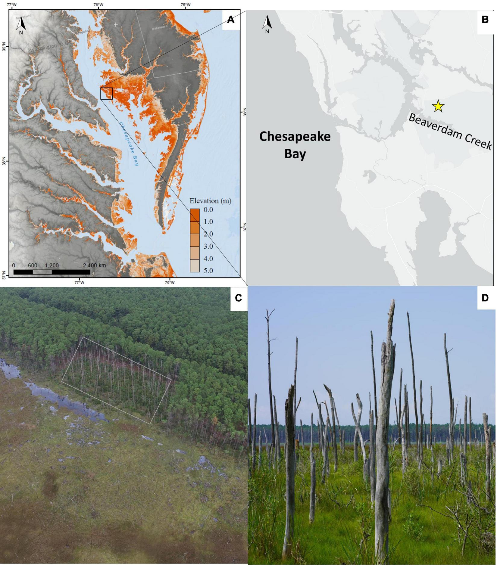
(A) Map of Chesapeake Bay region with an overlaid topobathymetric digital elevation model that displays elevation of areas <5.0 m NAVD88, from the United States Geological Survey’s Coastal National Elevation Database (Danielson and Tyler, 2016). Inset black box shows the position of the transgression experiment at the Blackwater National Wildlife Refuge on Maryland’s Eastern Shore of the Chesapeake Bay. (B) Site map showing Moneystump Swamp (yellow star) at the Blackwater National Wildlife Refuge situated on Beaverdam Creek, a tributary of the Chesapeake Bay, where the transgression experiment took place. (C) Aerial image of the Moneystump transgression experiment taken in 2018. The Control area is on the right side of the image where there are live trees, showing the natural gradient of pine forest transitioning to emergent brackish marsh. The overlayed rectangle shows the area where trees were killed via girdling (Credit: Tyler Messerschmidt). (D) Picture taken from within the ghost forest in the high marsh at Moneystump, looking parallel to the marsh forest boundary with the live forest to the right and the marsh extending out to the left. These trees are a sign of natural transgression that has occurred at this site (Credit: David C. Walters).
Moneystump Swamp, the USFWS BNWR property where this study takes place, is located on Beaverdam Creek which is a tributary of the Choptank River (Figure 1B). The average diurnal tide range at the site is 0.51 m, with a mean higher high water level of 0.34 m North American Vertical Datum 1988 (NAVD88), a mean water level of 0.12 m NAVD88, and an average salinity of 9.2 Practical Salinity Units (PSU) with a standard deviation of 3.3 PSU (Carr and Guntenspergen, 2020). The Moneystump property spans an elevation and ecological gradient that includes a large brackish marsh to the south and forested upland to the north. The vegetation transitions from low marsh to the south adjacent to Beaverdam Creek—dominated by Spartina alterniflora, Juncus roemerianus, and Schoenoplectus americanus—to high marsh to the north adjacent to the upland forest—dominated by Spartina patens and Distichlis spicata. Near the marsh-upland forest boundary (picture in Figure 1C) there is a prominent ghost forest, with standing dead trees in the high marsh community (Figure 1D). Then at the transition from the high marsh to the forest, a narrow band of shrubby species such as Morella cerifera and Iva frutescens dominates. The upland forest canopy is a nearly monoculture stand of Pinus taeda (a facultative species—Lichvar et al., 2016) with little understory growth (Figure 2, control), and an average upland slope of ∼0.008. The U.S. Geological Survey (USGS) established long-term surface elevation tables (SETs) at this site in the year 2000 along an elevation gradient from the low marsh into the upland. Over the course of 15 years monitoring the site, tree mortality and subsequent transition to wetland vegetation were observed in the higher elevation plots, identifying this site as an area of active transgression that would be an ideal location for a transgression study.
FIGURE 2
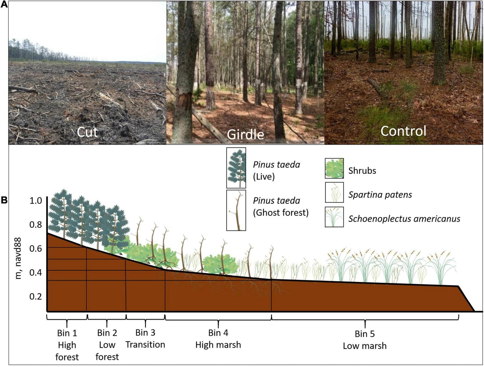
(A) Pictures taken from Moneystump Swamp transgression experiment (Cambridge, MD, United States) in the highest elevation bin in the Cut treatment area immediately after the trees were cut down in 2014, the Girdled treatment area immediately after the bark was stripped from the trees to slowly kill them in 2014, and the Control area where the trees were left alive (Photo credit: Patrick Brennand). (B) Schematic showing typical vegetation zonation at Moneystump along elevation gradient spanning from the low marsh into the high forest, and how those ecotones align with the elevation bins chosen for the transgression study (graphics from Integration and Application Network, ian.umces.edu/media-library).
Experimental Design
This experiment to understand the role of disturbance in marsh transgression was initiated in the summer of 2014 with the cutting and girdling of all live trees in designated areas at Moneystump Swamp by the USWS BWNR. The goal was to simulate a large-scale disturbance that could potentially induce changes in ecohydrological feedbacks such as changes in evapotranspiration rates that would influence salinity and inundation. To accomplish this, the size of the treatment areas had to be large beyond the scale of a mere mesocosm experiment. Therefore, with permission from the refuge, disturbance treatments were applied to whole sections of forest, killing off every tree within a large, forested area. In one 1.2-hectare portion of the forested study area, all trees were cut down by hand and harvested, in another 1.1-hectare portion, the trees were girdled at breast height by stripping the bark and cambium in a circle at the base of tree killing it slowly by terminating nutrient flow, and in another portion (1.1 hectares), the trees were left alive as a control area (Figure 2A). The scope of this large-scale environmental manipulation provides a unique opportunity to test the application of ecological theories such as press-pulse disturbance in a coastal forest setting. The two different treatments (Cut and Girdled) simulate natural tree mortality events where the effect of a gradual (Girdled) and immediate (Cut) change in conditions can be observed over time and can test the impact of tree mortality on migration and establishment of wetland vegetation upslope. In the case of the Cut treatment area, the removal of the forest canopy produces an immediate change in the light environment, such as would happen from a strong windstorm. Whereas in the case of the Girdled treatment area, the light environment changes more gradually as the foliage, limbs, and eventually tree trunks fall over time, thus gradually opening the canopy, as would happen from a storm surge that resulted in inundation and/or salt spray killing the trees. The marsh adjacent to each forested area in the study was left unchanged, as there were no trees to girdle or cut.
Each treatment area in the study area was then sub-divided into five elevation bins, reflecting the natural elevation-ecotone gradient (Figure 2B). The topographic elevation ranges were identified via Real Time Kinematic (RTK) surveying in the open canopy portions of the site where there is available satellite coverage, and a DNA03 Digital Laser Level referenced to known elevation benchmarks for the forested portion. The identified elevation ranges for each ecotone were: bin 1—high forest (0.60–0.72 m NAVD88), bin 2—low forest (0.54–0.60 m NAVD88), bin 3—transition (0.44–0.51 m NAVD88), bin 4—high marsh (0.39–0.43 m NAVD88), and bin 5—low marsh (0.31–0.40 m NAVD88) (Figure 2B and Supplementary Table 1). The average change in surveyed elevation from the marsh-forest transition in bin 3 to the high forest in bin 1 is 0.008. Across each elevation bin, in each treatment area, vegetation, water level, and light level were monitored.
Environmental Variables
Change in light level was monitored over the course of the experiment with HOBO Pendant light loggers, deployed at each vegetation plot attached to polyvinyl chloride (PVC) poles at a height of 1 m above the ground. Inundation was measured with an array of continuously recording HOBO and Solinst water level loggers deployed in slotted PVC groundwater wells. One well was placed in each elevation bin in each treatment area to track the influence of elevation and changes in vegetation on inundation. Continuously recording Solinst salinity loggers were deployed in 2020 in upland forest bin 1 of each treatment area and in transition bin 3 and low marsh bin 5 of the Control to monitor how salinity varies with elevation. Monitoring groundwater salinity provides information to determine if reduced transpiration due to tree mortality leads to an increase in saltwater intrusion into the upland, in addition to natural processes influencing saltwater intrusion such as sea level rise, storm surge, and drought.
Vegetation Field Surveys
Within each of the five elevation bins in each of the treatments, there were initially five vegetation plots established. However, upon conducting a higher precision integrated total station-RTK survey to better constrain the narrow elevation ranges, the plots were re-assigned such that there were four to six long-term vegetation plots in each elevation bin, for a total of 76 plots. Each vegetation plot consisted of a 1 m × 2 m quadrat for monitoring herbaceous vegetation and an overlapping 2 m × 5 m quadrat for monitoring shrubs, with the long side of plots oriented parallel to the elevation contour. For this study, shrubs were defined as woody plants that have a maximum height of less than 4 m tall with a diameter at breast height (DBH) of less than 2.5 cm. Over the 5-year duration of the experiment, the herbaceous vegetation was sampled three times per year in the spring, summer, and fall, while the shrub plots were sampled once per year in the fall.
At each plot, the presence of each species was recorded along with an estimate of the percent basal cover, or the proportion of the ground obscured by a species’ aboveground leaves and stems (Coulloudon et al., 1996). Percent cover was estimated following the cover class approach of the Daubenmire method (Daubenmire, 1959), with each species evaluated independently allowing for the possibility of the sum of cover classes in a plot exceeding 100% as plant covers from different species can overlap one another. The height of the tallest individual was also recorded for each species present. All the same measurements were recorded for the species that were identified in the shrub plot. For P. taeda, in addition to cover class and height, the total number of individuals rooted within the plot was counted for each survey, as it is the dominant tree species in this study and the density of individuals and rate of mortality is potentially an indicator of forest health and recovery.
Statistical Analyses
To compare the level of plant biodiversity across treatments, Shannon’s diversity index (H′) was calculated for each plot, as a function of the number of species in the plot (s) and the plant cover proportion (p) of each individual species (i) (Begon et al., 2006):
The presence and extent of wetland vegetation were analyzed through the use of the wetland prevalence index. Prevalence index (PI) is a metric of average species type which can be applied to wetland vegetation (Lichvar and Gillrich, 2014). PI is calculated by taking a weighted average of the cover class of all species (S) within a plot, weighted by wetland indicator status, from 1 for obligate wetland species (obl), to 2 for facultative wetland (facw), 3 for facultative (fac), 4 for facultative upland (facu), and 5 for upland (upl) (Lichvar et al., 2016):
Prevalence index values reflect the wetland indicator status of the vegetation community in the plot as a whole, from obligate wetland to upland vegetation. Values of less than 2.5 indicate a moderate probability that a vegetation community is wetland, and values less than 2 indicate a high probability that a vegetation community is wetland. H′ and PI were calculated for each vegetation survey that was done at each plot throughout the duration of the experiment. Analysis of variance was used to test for differences in PI and H′ across treatment areas and elevation bins.
Results
Light Environment
The measured light level was consistently low in the Control treatment with an intact overstory tree canopy. Only 21% of available light (determined by the maximum light levels recorded in un-shaded marsh plots) reached the 1 m level in high forest bin 1, the lowest light level recorded anywhere in the experiment. The next lowest light level was recorded in low forest bin 2 which is closer to the forest edge, and then in transition bin 3 where the canopy cover is thinnest (Supplementary Figure 1). No interannual trend in light environment was observed over the duration of the experiment in the Control. The Girdled forest initially had similar ranges of light levels as the Control (with light increasing from bin 1 to bin 3) then increased to maximum levels in 2018 as dead tree limbs fell and opened the canopy further, until it then began to decrease as new vegetation re-grew and shaded the sensors in 2019. The Cut forest by comparison experienced initially high light levels reaching close to the maximum light level in 2016 as the forest canopy was completely removed, then steadily decreased over time as vegetation continued to re-grow and shade the sensors. Overall, the trends show that the Cut forest resulted in an immediate increase in available light reaching the understory vegetation, while the Girdled forest resulted in a gradual increase in available light over several years.
Water Level and Salinity
Inundation measured from the groundwater wells was largely controlled by elevation (elevation effect P < 0.017) with average recorded inundation levels ranging from 50% in bin 5 to less than 1% in bins 1 and 2 (Supplementary Figure 2). There was no significant difference (F = 0.002, P = 0.998) between inundation levels in the different treatment areas in the upland elevation bins (bins 1, 2, and 3) with an average inundation of 1.2, 1.3, and 1.2% for the Control, Girdled, and Cut, respectively. Salinity values did not increase in the disturbed forest areas (bin 1) relative to the Control, with average values of 0.5 PSU, 0.8 PSU, and 1.2 PSU in the Cut, Girdled, and Control groundwater wells, respectively, and in fact Control salinity is greater than the salinity in the disturbed forest (P < 0.01). Groundwater salinity is greater in the marsh-upland forest transition (Control bin 3) at 9.3 PSU and greatest in the marsh (Control bin 5) at 11.2 PSU. Therefore, there was no treatment effect in the disturbed forest areas in flooding or salinity relative to the Control, but both salinity and inundation increase with decreasing elevation, regardless of treatment.
Forest Recovery
After the Cut and Girdled treatments were initiated in 2015, there were no live mature loblolly pines (P. taeda) remaining within the treatment areas (Figure 3, left). In the 5 years since, pine trees have largely recolonized the disturbed areas (Figure 3, right). Re-growing from seedlings, P. taeda has recovered to the point of once again being the dominant vegetation cover in the upland plots. P. taeda was never found above trace amounts in the low elevation plots (bins 4 and 5) where any seedling that did germinate died off shortly thereafter. Thus, the analysis of P. taeda growth and recovery focuses on the potential habitable range of the mid and high elevation plots (bins 1, 2, and 3).
FIGURE 3
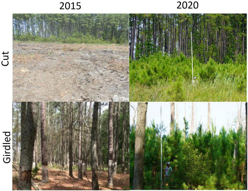
Shows change at Moneystump Swamp transgression experiment (Cambridge, MD, United States) from clear-cut state immediately after tree cutting (top left, photo credit: Patrick Brennand) to tree regrowth after 5 years post-recovery (top right, photo credit: David C. Walters) and change from standing dead pines immediately after girdling (bottom left, photo credit: Patrick Brennand) to tree regrowth amongst standing dead trunks after 5 years post-recovery (bottom right, photo credit: David C. Walters). 2020 photos include a 5 m staff positioned at the first row of live pines for scale.
In both the high forest and low forest understory (bins 1 and 2), P. taeda has shown a positive rate of recovery in cover and height (Figure 4). Cover increased linearly for the first 3 years as the seedlings took advantage of the increased availability of light and grew into saplings, before plateauing at a maximum level in 2018 (Figure 4, top left and middle left). In the transition zone (bin 3), P. taeda did not show any recovery via increasing cover in the Cut treatment (Figure 4, bottom left). However, in the Girdled treatment, P. taeda did recover to an average cover of 48% of the plot area in 2019. Ground cover of pines in the Control did not change from near zero, which is representative of trace amounts of sporadic seedlings, over the course of the experiment. However, the mature forest canopy was unchanged in the Control treatment with a sustained population of fully mature live P. taeda. The increase in cover of the P. taeda seedlings and saplings in the Cut and Girdled treatments reflects the recovery and recolonization of a healthy pine forest.
FIGURE 4
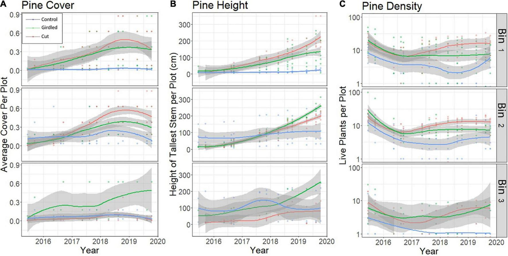
Multiple metrics to represent forest recovery (e.g., pine tree regrowth) at the Moneystump Swamp transgression experiment (Cambridge, MD, United States) over time for the high forest (bin 1), low forest (bin 2), and marsh forest transition (bin 3). (A) Change in cover class over time for understory P. taeda seedlings and saplings. (B) Change in height for tallest understory P. taeda in each plot. (C) Count of individuals in the understory, or density of P. taeda per 2 m2 plot. Each plot is color-coded for treatment, red is Cut, green is Girdled, and blue is Control. Trend lines depict Loess-smoothed local polynomial regression, with the shaded area around the trend lines showing the standard error.
The recovery of P. taeda can also be tracked through the increase in the height of the tallest individual of each plot (Figure 4, middle column). The increase in height is greatest in the Girdled and Cut treatments in upland bins 1 and 2 and the Girdled treatment transition bin 3, with an average height in 2019 of 2.0 m, and an average growth rate of 0.5 m/year. Control upland and transition (bins 1, 2, and 3) do not have discernible positive growth rates. This is because these plots contained understory P. taeda prior to the onset of the experiment that showed little to no signs of growth over the course of the experiment, as they are light limited due to forest canopy cover.
The count of individual P. taeda plants in the understory of each plot demonstrates the change in density over time as seedlings take root and die off. In the Cut and Girdled treatment, upland plots (bins 1 and 2), there were high recruitment rates at the beginning of the experiment (Figure 4, right column). After the first year, the density of seedlings in the Girdled upland plots decreased, as the increase in height and cover of the fastest growing individuals shades out the slower ones. Density of P. taeda is lower in the transition (bin 3) for each treatment area (Figure 4, bottom right) due to a high rate of mortality for seedlings, likely caused by increased inundation or salinity relative to the higher elevation bins. The light-limited Control plots also maintained consistently low density of P. taeda seedlings. Overall, these trends demonstrate that recruitment of P. taeda seedlings is sufficient for recruitment to outpace mortality in the upland (bins 1 and 2), leading to sapling growth on a trajectory toward full forest recovery.
Plant Community
The survey of the understory vegetation identified 70 distinct species and shows that the diversity is greatest in the upland and transition disturbed areas (i.e., the Cut and Girdled treatments) and marsh-upland forest transition across all treatment areas (one-way ANOVA P = 0.0003). Upland bins 1 and 2 in the Cut and Girdled, where forest disturbance allowed for more diverse herbaceous vegetation to colonize due to the opening of the canopy environment have an average Shannon’s Index of 1 (Supplementary Figure 3). Herbaceous grasses such as Panicum virgatum and Chasmanthium laxum are the most prevalent of the early colonizers of the disturbed areas, before they are outcompeted by the recovering P. taeda (Figure 5). In the marsh forest transition (bin 3) of both the disturbed areas and the Control, shrubs M. cerifera and I. frutescens are prevalent, but the most common species are still grasses such as P. virgatum and common high marsh grasses such as D. spicata and S. patens. The marsh (bins 4 and 5) contains a less diverse plant community with an average Shannon Index of 0.8, where only salt and inundation tolerant species are found, mostly S. patens and D. spicata in bin 4, and S. americanus in bin 5 (Figure 5). However, the upland Control plots (bins 1 and 2) have the least diversity with a Shannon’s Index of 0.4, and the vegetation community is dominated by mature loblolly pine P. taeda and the understory vegetation is made up of sporadic C. laxum and P. taeda seedlings. While the Cut and Girdled upland plots in bins 1 and 2 had greater diversity relative to the Control, wetland grasses were not among the species that colonized those areas.
FIGURE 5
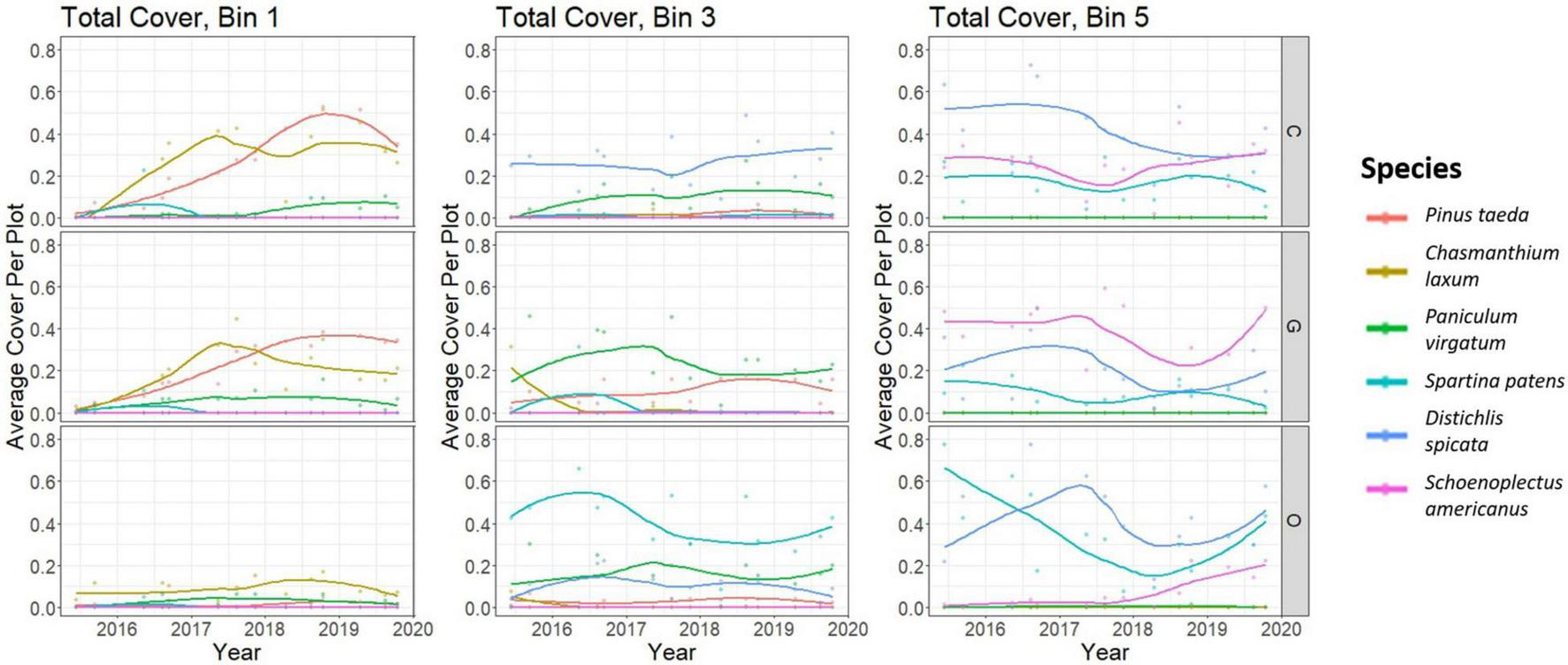
Plant cover over time for the six species with the highest total cover in the study area at Moneystump Swamp transgression experiment (Cambridge, MD, United States) over the course of the experiment (see legend), broken down by elevation bin (bin 1 on the left, bin 3 in the middle, and bin 5 on the right, showing only the high forest, transition, and low marsh, respectively, for simplicity) and treatment (Cut on top, Girdled in middle, and Control on bottom). A value of 1 represents complete coverage of all vegetation plots, and a value of zero represents complete absence from all vegetation plots. Trend lines depict Loess-smoothed local polynomial regression.
Hydrophytic Vegetation
The most prominent species that occurs in the upland environment in this study area is P. taeda, which is classified with a wetland indicator status of facultative (Lichvar et al., 2016). According to the National Wetland Plant List (Lichvar et al., 2016), a facultative status indicates an equal likelihood of occurring in either wetland or upland. The Prevalence Index (PI) provides a view of the gradient of hydrophytic vegetation that occurs within this site, since it subdivides hydrophytic vegetation along the gradient from facultative to obligate wetland species. According to the PI, wetland vegetation follows the expected elevation gradient across treatment areas and does not appear to have shifted over time (two-way ANOVA interaction effect P = 0.90, treatment effect P = 0.10, elevation effect P = 0.006, Figure 6). Bins 1 and 2 have the highest PI with no difference between treatments and an average of 2.6 ± 0.4, indicating a community with facultative species on average. The transition plots (bin 3) of the Girdled and Control treatments have the next highest PI’s with an average of 2.3 ± 0.6, indicating a vegetative community tipping toward facultative wetland species. The transition of the Cut treatment has the lowest PI of all the treatments outside of bins 4 and 5, with an average of 1.6 ± 0.5, which suggests a high probability that the site is a wetland. Of course, bins 4 and 5 have the lowest PI (1.3 ± 0.3), indicating mostly obligate wetland species. There was not a single vegetation survey over the 5 years of the experiment where the average PI of any of the Girdled, Cut, or Control upland bins (bins 1 and 2) was less than 2 (Supplementary Figure 4), indicating that wetland vegetation was not able to establish in the upland at any point.
FIGURE 6
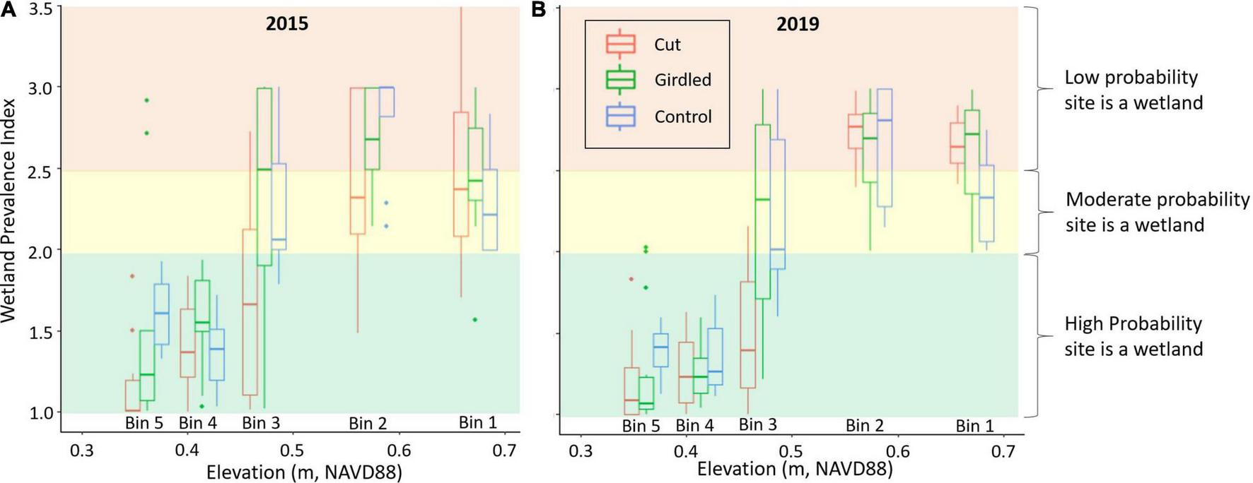
Wetland vegetation dynamics as a function of elevation and forest disturbance with Prevalence Index (PI) for the occurrence of hydrophytic vegetation versus elevation, color-coded by treatment area for (A) the first year of the experiment (2015) and (B) the last year (2019). PI values greater than 2.5 indicate a low probability a site is a wetland, values between 2 and 2.5 indicate a good probability that a site is a wetland, and values less than 2 indicate a high probability that a site is a wetland. Boxplot centerline represents the median value of the data, the upper and lower box sides represent the 25th and 75th percentile datapoints, the whiskers extend to the largest and smallest values within the 1.5 interquartile range of the 25th and 75th percentile, and all remaining points are plotted as outliers.
The disturbed forest plots in Cut and Girdled upland elevation bins 1 and 2 showed no trend toward the occurrence of more wetland vegetation over time (Figure 7). Several individual plots in the Cut and Girdled upland bins recorded PI’s in the range of wetland vegetation (1.5–2) within the first 2 years of the experiment, but on average the PIs were no different or greater than those in the Control plots. There was a greater range in PI of the experiment in the Cut and Girdled prior to 2017—there were plots with PI values greater than 3 and less than 2—as the diversity was higher before pine recovery had established as the dominant cover type (Figure 5). From 2017 onward, no individual plot in the upland elevation bins 1 and 2 recorded a PI of less than 2 (Figure 7), as the pine saplings shaded out any potential for wetland species colonization and the vegetation among the plots became more uniform.
FIGURE 7
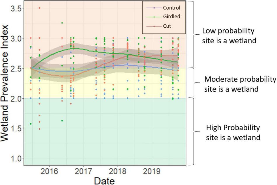
Change in Wetland Prevalence Index (PI) over time in upland elevation bins 1 and 2, color-coded by treatment. PI values greater than 2.5 indicate a low probability a site is a wetland, values between 2 and 2.5 indicate a good probability that a site is a wetland, and values less than 2 indicate a high probability that a site is a wetland. Points represent the PI calculated from each vegetation survey conducted for each single vegetation plot in upland bins 1 and 2. Trend lines depict Loess-smoothed local polynomial regression, with the shaded area around the trend lines showing the standard error.
Discussion
Positive feedbacks between limiting resources and system state can lead to ecosystem dynamics that exhibit alternative stable states (Wilson and Agnew, 1992). Alternative stable state dynamics in an ecosystem are associated with the potential for strong non-linear behavior, whereby a small change in an environmental driver can lead to rapid shifts in ecosystem structure. Moreover, these systems are known to possess limited resilience in the sense that a disturbance or sequence of disturbances could shift the system past some critical threshold into an alternative state, whereby the original system state is unable to recover even if the disturbance is removed (Scheffer et al., 2001; van Nes and Scheffer, 2004). However, in this study, we observed a forest in a stable state which was able to recover following disturbance, suggesting that there are negative feedbacks increasing resiliency.
Across the marsh-upland forest, ecotones are gradients in light availability, inundation, and salinity which are affected by both the state of the system and environmental drivers. For example, near the edge of tidal inundation, overstory tree canopy loss could lead to increased salinity due to increased surface evaporation leading to potential further canopy loss or tree mortality as well as the inhibition of pine seedling establishment (Kurz and Wagner, 1957). Halophytic vegetation can contribute further to soil salinization (Sternberg et al., 2007; Wendelberger and Richards, 2017). Alternately, increased evapotranspiration due to the presence of herbaceous vegetation could lower the water table helping to facilitate seedling establishment (Poulter et al., 2009), which could be the cause of reduced groundwater salinity in the disturbed forest plots in our experiment. Our experiment uniquely tested the presence of alternative stable states by disturbing an established forest canopy (state 1) and measuring potential marsh establishment (state 2) at a scale large enough (>3 hectares of pre-treatment forested area) to potentially influence the light and water resources thought to govern the transition between states. However, we observed no difference in inundation between treatment areas, decreased groundwater salinity in the disturbed forest areas relative to the control, rapid pine re-growth (Figure 4) and little change in wetland prevalence across zones (Figure 6), indicating that dominant system states recovered quickly following disturbance, and that disturbance alone was not sufficient to induce an ecosystem state change.
The interplay of positive feedbacks, ecosystem state, and environmental drivers can lead to an “ecological ratchet” conceptual model of marsh transgression (Fagherazzi et al., 2019), whereby the coastal forest exists in zones determined by forest regeneration (i.e., the regenerative zone), or where seedling establishment ceases but mature trees are able to persist (i.e., the persistence zone). In this experiment, manipulated plots showed pine forest recovery in high elevation bins and the increase in height of the pine seedlings and subsequent saplings in the Girdled and Cut areas relative to the Control illustrates the trajectory of the plant community toward mature adult pines (Figure 4). This recovery suggests that these upper elevation bins exist within the regenerative zone where seedlings are able to establish and forest succession can occur (Kearney et al., 2019). This experiment is an ideal test for the concept of a persistence zone because the light restriction that might otherwise prevent regeneration has been removed. However, across this low slope environment, the only location where the removal of mature trees did not result in complete regeneration was in the transition bin 3 (Figure 6), but this transition zone is located at the forest edge where removal of the remaining forest canopy had less of an impact on the light environment (Supplementary Figure 1). Moreover, the transition zone is a relatively narrow zone characterized by edge effects, and is not an extensive persistent zone where adult trees are underlain by marsh vegetation, suggesting that a prior transgressive event may have already pushed the trailing edge of the persistence zone up into the leading boundary of transgression, but further data are needed to test this hypothesis. As such, there is at most only a narrow band of elevation at this site where there is potential for wetland species to colonize and persist in the forested areas under current environmental conditions (Jackson et al., 2009). The lack of strong coastal marsh plant species response suggests that the shift in biotic and abiotic factors in the upper elevation bins of the experiment was not enough, and/or not fast enough, to induce a state change (Field et al., 2016).
This study site falls well within the range of low slope environments around the Chesapeake Bay where transgressions can occur rapidly (Schieder and Kirwan, 2019; Molino et al., 2021). However, it has been noted that even in low slope environments, transgression sometimes occurs slowly into forested upland areas (Schieder et al., 2018). This lack of transgression is likely not due to seedbank limitation as marsh species exist in the seedbank of the upland forest environment within this region and this study site (Kottler and Gedan, 2020), suggesting that competition between marsh and upland vegetation, rather than inadequate seed supply, may have limited the ability of marsh vegetation to become established in our experiment. While the opening of the canopy provided an opportunity for marsh species colonization, increases in the light environment and consequent environmental changes were not sufficient to push the system past a critical threshold where marsh species could establish and thrive as evidenced by the lack of marsh species across all upland manipulation and control plots (Figure 7). Even in elevation bin 3, where the transition between marsh vegetation and forest vegetation occurs and both upland and marsh species are found, removal of the canopy did not shift the vegetation composition (Figure 5). This study de-emphasizes the potential importance of episodic disturbance events that drive transgression on the century time-scale (Young, 1995), accompanied by changes in salinity and inundation.
Pulse disturbances, including storms (Gardner et al., 1992; Ross et al., 2009; Wang and Xu, 2009), drought (Desantis et al., 2007; NeSmith et al., 2018; Ury et al., 2021), wrack deposition (Tate and Battaglia, 2013), and changing hydroperiod (Antonellini and Mollema, 2010), are viewed as a first step in the conversion of coastal forests to salt marsh. However, press disturbances—such as gradual saltwater intrusion and changes in flooding—interact with pulse disturbances because they alter the recovery from the pulse disturbance by changing the environmental setting of the forested habitat so that tree regeneration fails and halophyte vegetation successfully colonizes a site (Fagherazzi et al., 2019). Despite the disturbance treatments, transgression was not facilitated in this experiment, likely due to a lack of enabling environmental stressors. Press stressors such as inundation level and soil salinization must cross a critical environmental threshold before wetland vegetation can outcompete tree seedling recovery. Wasson et al. (2013) observed a gradual movement of a total of 1 m of the marsh-upland forest transition ecotone over the course of a 10-year period in a California estuary, which was found to correlate with an increase in inundation from 2 to 4%. Despite very different slope conditions, this aligns well with the 3% inundation rate observed in the transition ecotone in our study, which also compares closely with the 3.6% inundation where Anisfeld et al. (2017) observed a transition from marsh to upland vegetation zones in a Long Island Sound salt marsh. This suggests that areas with inundations of less than 2% are unlikely to transition to marsh following a disturbance. However, elevation change and the water level inundation signal can feedback on one another, due to potential root zone collapse following forest disturbance (Cahoon et al., 2003). Alternatively, forest thinning has been shown to lead to elevation gain due to increased root production by colonizing understory vegetation (Chen et al., 2021). Also, certain seedlings of coastal tree species have been killed by high saline soils in north Florida, but then resprouted after salinity decreased when flushed with freshwater (Williams et al., 1998). This effect of saline soils suggests that the deposition of salt following storm surges is an important aspect of disturbance events, that leads to transgression, because even if salt deposition occurs in an area with low frequency of tidal inundation, it can create a delay in the recovery of tree seedlings that allows time for marsh plants to establish.
Loss of the forest canopy removes light limitation and results in the germination and establishment of a greater variety of plant species, suggesting that aboveground light competition outweighs belowground nutrient competition between species. However, if the overstory tree canopy recovers, the subsequent light limitation results in the establishment of a shade-tolerant plant community, regeneration of overstory tree species, and loss of marsh species which are shade intolerant. However, changes in salinity and flooding (press disturbances) can inhibit the regeneration of tree seedlings and allow marsh plants to become established. Over the duration of this experiment, loss of the tree canopy led to an initial increase of plant species diversity, but the absence of changes in soil salinity or site inundation (pressure disturbances) led to the germination and growth of the overstory tree species (P. taeda) and shading of the plant species that established initially (Figure 6).
A current paradigm in coastal ecology is that coastal forests follow a punctuated equilibrium response to sea level rise, where adult trees are generally resistant to gradual increases in inundation and salinity, and that rapid retreat follows episodic disturbance events (Williams et al., 1999; Fagherazzi et al., 2019; Kirwan and Gedan, 2019). For example, fast periods of forest retreat punctuated gradual forest retreat in portions of the Chesapeake Bay and Albemarle-Pamlico Sound estuaries following Hurricanes Katrina and Irene, respectively (Schieder and Kirwan, 2019; Ury et al., 2021). However, recent numerical modeling suggests that the interplay between sea level rise and disturbance events depends on local conditions such as topographic slope and the rate of sea level rise, and emphasizes the potential for regeneration of forests after disturbance events (Carr et al., 2020). Our large-scale field experiment uniquely disturbed the forest canopy without directly altering environmental factors such as salinity that would accompany sea level rise in natural systems, and therefore isolates the effect of disturbance alone. Interestingly, we found increased light availability led primarily to a release of upland rather than wetland plant species, and that potential ecohydrological feedbacks associated with tree mortality were not sufficient to induce state changes. Thus, our work illustrated rapid recovery of a forested ecosystem, and suggests that disturbance alone is not sufficient for transgression to occur.
Publisher’s Note
All claims expressed in this article are solely those of the authors and do not necessarily represent those of their affiliated organizations, or those of the publisher, the editors and the reviewers. Any product that may be evaluated in this article, or claim that may be made by its manufacturer, is not guaranteed or endorsed by the publisher.
Statements
Data availability statement
The datasets presented in this study can be found in the online repository USGS ScienceBase Catalog: https://www.sciencebase.gov/catalog/item/6196b7cad34eb622f691ac94 and doi: 10.5066/P9V4NJXW.
Author contributions
All authors contributed to writing the manuscript and provided valuable input to the project at various stages.
Funding
We acknowledge support from the USGS Climate Research and Development and Ecosystems Programs.
Acknowledgments
We thank the staff at Blackwater National Wildlife Refuge for their support of this project. Any use of trade, firm, or product names is for descriptive purposes only and does not imply endorsement by the U.S. Government.
Conflict of interest
The authors declare that the research was conducted in the absence of any commercial or financial relationships that could be construed as a potential conflict of interest.
Supplementary material
The Supplementary Material for this article can be found online at: https://www.frontiersin.org/articles/10.3389/fmars.2021.782643/full#supplementary-material
References
1
Anisfeld S. C. Cooper K. R. Kemp A. C. (2017). Upslope development of a tidal marsh as a function of upland land use.Glob. Chang. Biol.23755–766. 10.1111/gcb.13398
2
Antonellini M. Mollema P. N. (2010). Impact of groundwater salinity on vegetation species richness in the coastal pine forests and wetlands of Ravenna. Italy.Ecol. Eng.361201–1211. 10.1016/j.ecoleng.2009.12.007
3
Begon M. Townsend C. Harper J. (2006). Ecology: From Individuals to Ecosystems.New York, NY: Wiley.
4
Bender E. A. Case T. J. Gilpin M. E. (1984). Perturbation experiments in community ecology: theory and practice.Ecology651–13. 10.2307/1939452
5
Boesch D. F. Galloway G. E. Zoë P. Johnson P. Kopp R. E. Li M. et al (2018). Sea-level Rise: Projections for Maryland.Cambridge, MD: University of Maryland Center for Environmental Science.
6
Boon J. D. Brubaker J. M. Forrest D. R. (2010). Chesapeake Bay Land Subsidence and Sea Level Change: An Evaluation of Past and Present Trends and Future Outlook.Washington, DC: U.S. Global Change Research Program.
7
Borchert S. M. Osland M. J. Enwright N. M. Griffith K. T. (2018). Coastal wetland adaptation to sea level rise: quantifying potential for landward migration and coastal squeeze.J. Appl. Ecol.552876–2887. 10.1111/1365-2664.13169
8
Brinson M. M. Christian R. R. Blum L. K. (1995). Multiple states in the sea-level induced transition from terrestrial forest to estuary.Estuaries18648–659. 10.2307/1352383
9
Cahoon D. R. Hensel P. Rybczyk J. Kee K. L. M. Proffitt C. E. Perez B. C. (2003). Mass tree mortality leads to mangrove peat collapse at Bay Islands, Honduras after Hurricane Mitch.J. Ecol.911093–1105.
10
Carr J. Guntenspergen G. Kirwan M. (2020). Modeling marsh-forest boundary transgression in response to storms and sea-level rise.Geophys. Res. Lett.47:e2020GL088998. 10.1029/2020GL088998
11
Carr J. A. Guntenspergen G. R. (2020). Water Levels (November 11 2016 Through November 11 2017) for Four Wells: From Upland to Marsh, Moneystump Marsh, Blackwater National Wildlife Refuge.Maryland: U.S. Geological Survey data release.
12
Chen L. Lin Q. Krauss K. W. Zhang Y. Cormier N. Yang Q. (2021). Forest thinning in the seaward fringe speeds up surface elevation increment and carbon accumulation in managed mangrove forests.J. Appl. Ecol.581899–1909. 10.1111/1365-2664.13939
13
Coulloudon B. Eshelman K. Gianola J. Habich N. Hughes L. Johnson C. et al (1996). Sampling Vegetation Attributes.Scotts Valley, CA: CreateSpace Independent Publishing Platform.
14
Danielson J. Tyler D. (2016). Topobathymetric Model for Chesapeake Bay Region - District of Columbia, State of Delaware, Maryland, Pennsylvania, and Virginia, 1859 to 2015. Available online at: https://topotools.cr.usgs.gov/topobathy_viewer/dwndata.htm(accessed on 29 January 2020).
15
Daubenmire R. F. (1959). A canopy-cover method of vegetation analysis.Northwest Sci.3343–46.
16
Desantis L. Bhotika S. Williams K. Putz F. (2007). Sea - level rise and drought interactions accelerate forest decline on the Gulf Sea-level rise and drought interactions accelerate forest decline on the Gulf Coast of Florida, USA.Glob. Chang. Biol.132349–2360. 10.1111/j.1365-2486.2007.01440.x
17
Enwright N. M. Griffith K. T. Osland M. J. (2016). Barriers to and opportunities for landward migration of coastal wetlands with sea-level rise.Front. Ecol. Environ.14:307–316. 10.1002/fee.1282
18
Fagherazzi S. Anisfeld S. C. Blum L. K. Long E. V. Feagin R. A. Fernandes A. et al (2019). Sea level rise and the dynamics of the marsh-upland boundary.Front. Environ. Sci.7:25. 10.3389/fenvs.2019.00025
19
Field C. R. Dayer A. A. Elphick C. S. Kareiva P. (2017b). Landowner behavior can determine the success of conservation strategies for ecosystem migration under sea-level rise.PNAS1149134–9139. 10.7910/DVN/NAKYZD
20
Field C. R. Bayard T. S. Gjerdrum C. Hill J. M. Meiman S. Elphick C. S. (2017a). High-resolution tide projections reveal extinction threshold in response to sea-level rise.Glob. Chang. Biol.232058–2070. 10.1111/gcb.13519
21
Field C. R. Gjerdrum C. Elphick C. S. (2016). Forest resistance to sea-level rise prevents landward migration of tidal marsh.Biol. Conserv.201363–369. 10.1016/j.biocon.2016.07.035
22
Gardner L. R. Michener W. K. Williams T. M. Blood E. R. Kjerfve B. Smock D. J. et al (1992). Disturbance effects of Hurricane Hugo on a pristine coastal landscape: North Inlet, South Carolina, USA.Netherlands J. Sea Res.30249–263.
23
Gedan K. B. Fernández-Pascual E. (2019). Salt marsh migration into salinized agricultural fields: a novel assembly of plant communities.J. Veg. Sci.301007–1016. 10.1111/jvs.12774
24
Jackson S. T. Betancourt J. L. Booth R. K. Gray S. T. (2009). Ecology and the ratchet of events: climate variability, niche dimensions, and species distributions.Proc. Natl. Acad. Sci. U.S.A.10619685–19692. 10.1073/pnas.0901644106
25
Jobe J. G. D. Gedan K. (2021). Species-specific responses of a marsh-forest ecotone plant community responding to climate change.Ecology1021–11. 10.1002/ecy.3296
26
Kearney W. S. Fernandes A. Fagherazzi S. (2019). Sea-level rise and storm surges structure coastal forests into persistence and regeneration niches.PLoS One14:e0215977. 10.1371/journal.pone.0215977
27
Kirwan M. L. Gedan K. B. (2019). Sea-level driven land conversion and the formation of ghost forests.Nat. Clim. Change9450–457. 10.1038/s41558-019-0488-7
28
Kirwan M. L. Walters D. C. Reay W. G. Carr J. A. (2016). Sea level driven marsh expansion in a coupled model of marsh erosion and migration.Geophys. Res. Lett.434366–4373. 10.1002/2016GL068507
29
Kottler E. J. Gedan K. (2020). Seeds of change: characterizing the soil seed bank of a migrating salt marsh.Ann. Bot.125335–344. 10.1093/aob/mcz133
30
Kurz H. Wagner K. (1957). Tidal Marshes of the Gulf and Atlantic Coasts of Northern Florida and Charleston, South Carolina: Geology, Elevations, Soil Factors, Water Relations, Plant Zonation and Succession.Tallahassee: Florida State University.
31
Lichvar R. W. Banks D. L. Kirchner W. N. Melvin N. C. (2016). 2016 national wetland plant list.Phytoneuron301–17.
32
Lichvar R. W. Gillrich J. J. (2014). Examining Discrepancies Among Three Methods Used to Make Hydrophytic Vegetation Determinations for Wetland Delineation Purposes.Hanover, NH: US Army Engine Research and Development Center.
33
Mitchell M. Herman J. Bilkovic D. M. Hershner C. (2017). Marsh persistence under sea-level rise is controlled by multiple, geologically variable stressors.Ecosyst. Heal. Sustain.3:1379888. 10.1080/20964129.2017.1396009
34
Molino G. D. Defne Z. Aretxabaleta A. L. Ganju N. K. Carr J. A. (2021). Quantifying slopes as a driver of forest to marsh conversion using geospatial techniques: application to Chesapeake Bay Coastal-Plain, United States.Front. Environ. Sci.9:1–13. 10.3389/fenvs.2021.616319
35
NeSmith J. E. Alba C. Flory S. L. (2018). Experimental drought and plant invasion additively suppress primary pine species of southeastern US forests.For. Ecol. Manag.411158–165. 10.1016/j.foreco.2017.12.045
36
Poulter B. Christensen N. L. Qian S. S. (2008). Tolerance of Pinus taeda and Pinus serotina to low salinity and flooding: implications for equilibrium vegetation dynamics.J. Veg. Sci.1915–22. 10.3170/2007-8-18410
37
Poulter B. Qian S. S. Christensen N. L. (2009). Determinants of coastal treeline and the role of abiotic and biotic interactions.Plant Ecol.20255–66. 10.1007/s11258-008-9465-3
38
Raabe E. A. Stumpf R. P. (2016). Expansion of tidal marsh in response to sea-level rise: Gulf Coast of Florida, USA.Estuar. Coasts39145–157. 10.1007/s12237-015-9974-y
39
Ross M. S. O’Brien J. J. Ford R. G. Zhang K. Morkill A. (2009). Disturbance and the rising tide: the challenge of biodiversity management on low-island ecosystems.Front. Ecol. Environ.7:471–478. 10.1890/070221
40
Sallenger A. H. Doran K. S. Howd P. A. (2012). Hotspot of accelerated sea-level rise on the Atlantic coast of North America.Nat. Clim. Chang.2884–888. 10.1038/nclimate1597
41
Scheffer M. Carpenter S. Foley J. A. Folke C. Walker B. (2001). Catastrophic shifts in ecosystems.Nature413591–596. 10.1038/35098000
42
Schepers L. Kirwan M. Guntenspergen G. Temmerman S. (2017). Spatio-temporal development of vegetation die-off in a submerging coastal marsh.Limnol. Oceanogr.62137–150. 10.1002/lno.10381
43
Schieder N. W. Kirwan M. L. (2019). Sea-level driven acceleration in coastal forest retreat.Geology471151–1155. 10.1130/G46607.1
44
Schieder N. W. Walters D. C. Kirwan M. L. (2018). Massive upland to wetland conversion compensated for historical marsh loss in Chesapeake Bay, USA.Estuar. Coasts41940–951. 10.1007/s12237-017-0336-9
45
Schuerch M. Spencer T. Temmerman S. Kirwan M. L. Wolff C. Lincke D. et al (2018). Future response of global coastal wetlands to sea-level rise.Nature561231–234. 10.1038/s41586-018-0476-5
46
Scott M. McDermott L. Silva E. Watson E. (2009). Project Report: Digital Spatial Data Capture of Marsh Extent in Blackwater National Wildlife Refuge, 1938 and 2006.Salisbury, MD: Eastern Shore Regional GIS Cooperative.
47
Smith J. A. M. (2013). The role of phragmites australis in mediating inland salt marsh migration in a mid-atlantic estuary.PLoS One8:e0065091. 10.1371/journal.pone.0065091
48
Smith J. A. M. Hafner S. F. Niles L. J. (2017). The impact of past management practices on tidal marsh resilience to sea level rise in the Delaware Estuary.Ocean Coast. Manag.14933–41. 10.1016/j.ocecoaman.2017.09.010
49
Song J. Fu X. Wang R. Peng Z. R. Gu Z. (2018). Does planned retreat matter? Investigating land use change under the impacts of flooding induced by sea level rise.Mitig. Adapt. Strateg. Glob. Chang.23703–733. 10.1007/s11027-017-9756-x
50
Sternberg L. D. S. L. Teh S. Y. Ewe S. M. L. Miralles-Wilhelm F. DeAngelis D. L. (2007). Competition between hardwood hammocks and mangroves.Ecosystems10648–660. 10.1007/s10021-007-9050-y
51
Stevenson J. C. Ward L. G. Kearney M. S. (1986). Vertical accretion in marshes with varying rates of sea level rise.Estuar. Var.0241–259. 10.1016/b978-0-12-761890-6.50020-4
52
Taillie P. J. Moorman C. E. Poulter B. Ardón M. Emanuel R. E. (2019). Decadal-scale vegetation change driven by salinity at leading edge of rising sea level.Ecosystems221918–1930. 10.1007/s10021-019-00382-w
53
Tate A. S. Battaglia L. L. (2013). Community disassembly and reassembly following experimental storm surge and wrack application.J. Veg. Sci.2446–57. 10.1111/j.1654-1103.2012.01447.x
54
Ury E. A. Yang X. Wright J. P. Bernhardt E. S. (2021). Rapid deforestation of a coastal landscape driven by sea level rise and extreme events.Ecol. Appl.01–11. 10.1002/eap.2339
55
van Nes E. H. Scheffer M. (2004). Large species shifts triggered by small forces.Am. Nat.164255–266. 10.1086/422204
56
Wang F. Xu Y. J. (2009). Hurricane Katrina-induced forest damage in relation to ecological factors at landscape scale.Environ. Monit. Assess.156491–507. 10.1007/s10661-008-0500-6
57
Wasson K. Woolfolk A. Fresquez C. (2013). Ecotones as indicators of changing environmental conditions: rapid migration of salt marsh-upland boundaries.Estuar. Coasts36654–664. 10.1007/s12237-013-9601-8
58
Wendelberger K. S. Richards J. H. (2017). Halophytes can salinize soil when competing with glycophytes, intensifying effects of sea level rise in coastal communities.Oecologia184729–737. 10.1007/s00442-017-3896-2
59
Williams K. Ewel K. C. Stumpf R. P. Putz F. E. Workman T. W. Williams K. et al (1999). Sea-level rise and coastal forest retreat on the West Coast of Florida, USA.Ecology802045–2063.
60
Williams K. Meads M. V. Sauerbrey D. A. (1998). The roles of seedling salt tolerance and resprouting in forest zonation on the west coast of Florida, USA.Am. J. Bot.851745–1752. 10.2307/2446509
61
Wilson J. B. Agnew A. D. (1992). Positive-feedback switches in plant communities.Adv. Ecol. Res.23263–336. 10.1016/S0065-2504(08)60149-X
62
Young R. S. (1995). Coastal Wetland Dynamics in Response to Sea-Level Rise: Transgression and Erosion.Doctoral Dissertation.
Summary
Keywords
transgression, sea level rise, marsh, forest, ecology
Citation
Walters DC, Carr JA, Hockaday A, Jones JA, McFarland E, Kovalenko KE, Kirwan ML, Cahoon DR and Guntenspergen GR (2021) Experimental Tree Mortality Does Not Induce Marsh Transgression in a Chesapeake Bay Low-Lying Coastal Forest. Front. Mar. Sci. 8:782643. doi: 10.3389/fmars.2021.782643
Received
24 September 2021
Accepted
09 November 2021
Published
10 December 2021
Volume
8 - 2021
Edited by
Zhan Hu, Sun Yat-sen University, China
Reviewed by
Keryn Gedan, George Washington University, United States; Luzhen Chen, Xiamen University, China
Updates
Copyright
© 2021 Walters, Carr, Hockaday, Jones, McFarland, Kovalenko, Kirwan, Cahoon and Guntenspergen.
This is an open-access article distributed under the terms of the Creative Commons Attribution License (CC BY). The use, distribution or reproduction in other forums is permitted, provided the original author(s) and the copyright owner(s) are credited and that the original publication in this journal is cited, in accordance with accepted academic practice. No use, distribution or reproduction is permitted which does not comply with these terms.
*Correspondence: David C. Walters, davidwalters@usgs.gov
This article was submitted to Coastal Ocean Processes, a section of the journal Frontiers in Marine Science
Disclaimer
All claims expressed in this article are solely those of the authors and do not necessarily represent those of their affiliated organizations, or those of the publisher, the editors and the reviewers. Any product that may be evaluated in this article or claim that may be made by its manufacturer is not guaranteed or endorsed by the publisher.