Abstract
Iodine affects the radiative budget and the oxidative capacity of the atmosphere and is consequently involved in important climate feedbacks. A fraction of the iodine emitted by oceans ends up in aerosols, where complex halogen chemistry regulates the recycling of iodine to the gas-phase where it effectively destroys ozone. The iodine speciation and major ion composition of aerosol samples collected during four cruises in the East and West Pacific and Indian Oceans was studied to understand the influences on iodine’s gas-aerosol phase recycling. A significant inverse relationship exists between iodide (I–) and iodate (IO3–) proportions in both fine and coarse mode aerosols, with a relatively constant soluble organic iodine (SOI) fraction of 19.8% (median) for fine and coarse mode samples of all cruises combined. Consistent with previous work on the Atlantic Ocean, this work further provides observational support that IO3– reduction is attributed to aerosol acidity, which is associated to smaller aerosol particles and air masses that have been influenced by anthropogenic emissions. Significant correlations are found between SOI and I–, which supports hypotheses that SOI may be a source for I–. This data contributes to a growing observational dataset on aerosol iodine speciation and provides evidence for relatively constant proportions of iodine species in unpolluted marine aerosols. Future development in our understanding of iodine speciation depends on aerosol pH measurements and unravelling the complex composition of SOI in aerosols.
Introduction
Iodine is ubiquitous in the troposphere where it plays an active role in atmospheric chemistry and important climate feedbacks (Prados-Roman et al., 2015a). Its volatile compounds contribute to aerosol particle formation mechanisms that affect the atmospheric radiative budget (O’Dowd et al., 2002; Read et al., 2008). It has furthermore been recognised to alter the oxidative capacity of the atmosphere by significantly destroying ozone (a pollutant) in the lower troposphere (Chameides and Davis, 1980; Chatfield and Crutzen, 1990; Davis et al., 1996; Mahajan et al., 2010). Biologically, iodine is a crucial element for mammalian metabolism (Whitehead, 1984), entering the food chain through atmospheric deposition on soil and crops.
The dominant source of iodine in the atmosphere is the surface ocean through biotic and abiotic processes (Mahajan et al., 2012). Volatile iodine compounds are released mostly in inorganic form, such as molecular iodine (I2) and hypoiodous acid (HOI) (Carpenter et al., 2013; Prados-Roman et al., 2015b), but also as organic iodocarbons, such as CH3I and CH2I2 (Klick and Abrahamsson, 1992; Moore and Tokarczyk, 1992; Schall et al., 1997; Martino et al., 2009; Jones et al., 2010). Rapid photolysis in the atmosphere releases the iodine atoms from these compounds, which subsequently participate in efficient ozone destruction cycles (Saiz-Lopez et al., 2012a,b).
Aerosols take up iodine, temporarily inhibiting its role in ozone destruction before recycling it back to the gas-phase. Aerosol composition, chemistry, and iodine speciation regulate the efficiency of iodine recycling and thus also the effect on ozone concentrations in the marine boundary layer (MBL) (Vogt et al., 1999; McFiggans et al., 2000; Hoffmann et al., 2001), and transport to continents where it may be deposited (Baker et al., 2001). Understanding aerosol iodine speciation in aerosols is therefore important to accurately reproduce ozone concentrations with atmospheric models, and to comprehend its effect on global radiation, climate, and feedbacks (Saiz-Lopez et al., 2012b).
Total soluble iodine (TSI) in aerosols in the MBL is characterised by geographical variability, being latitudinally and longitudinally dependent on global ocean temperature, seawater iodine content, and atmospheric ozone (Gómez Martín et al., 2021). TSI itself consists of iodide (I–), iodate (IO3–), and soluble organic iodine (SOI). Other iodine species, such as HOI or I2, are considered reactive or insoluble and therefore are not expected to be detectable in aerosols (Saiz-Lopez et al., 2012a).
Models have struggled to reproduce the variable iodine speciation, and thus also the MBL ozone levels, reported by observational studies (Gäbler and Heumann, 1993; Wimschneider and Heumann, 1995; Baker, 2004). Challenges in improving our understanding of the complex iodine chemistry in the MBL include sparsity of observational data and use of iodine speciation-altering extraction methods for samples (Xu S. Q. et al., 2010; Yodle and Baker, 2019).
We present aerosol iodine speciation data from three different major ocean basins: the West Pacific Ocean and, for the first time, the East Pacific Ocean and Indian Ocean. We investigate the consistency of the results with recent advancements in our understanding of aerosol iodine chemistry, including the role of SOI as a missing source for I– (Baker, 2005; Pechtl et al., 2007) and possible explanations for the variability in the IO3– concentrations.
Materials and Methods
Sample Collection
We present aerosol data obtained during four expeditions at sea between October 2009 and July 2017: TransBrom, SHIVA, OASIS, and M138 (Figure 1 and Table 1). The aerosol speciation results for the SHIVA campaign have previously been published by Yodle and Baker (2019), for which data can be found here: Baker and Yodle (2018). Results for TransBrom (Baker and Yodle, 2021b), OASIS (Baker and Droste, 2021), and M138 (Baker, 2021) can be found in the PANGAEA® database.
FIGURE 1
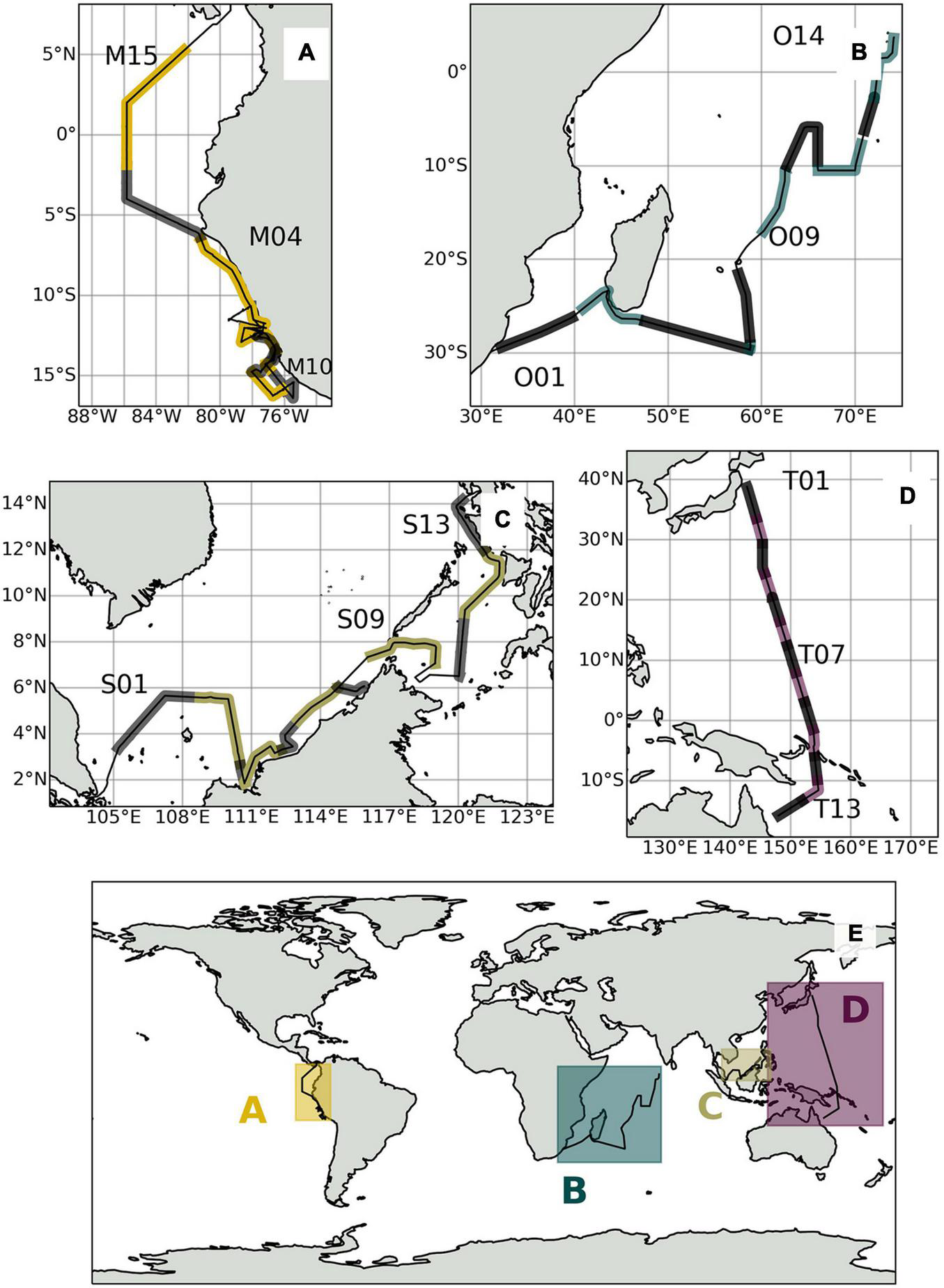
(E) Global overview map of expedition tracks and sampling locations shown in alternating lighter and darker shades for (A) M138, (B) OASIS, (C) SHIVA, and (D) TransBrom.
TABLE 1
| Expedition | Dates | Aerosol fractions collected | Aerosol Filters | Reference | Ship |
| TransBrom | 09.10.2009–24.10.2009 | Fine/coarse | Cellulose (Whatman 41) | Quack and Krüger, 2010; Martino et al., 2014 | FS Sonne SO202 |
| SHIVA | 15.11.2011–29.11.2011 | Bulk | Glass microfiber | Quack and Krüger, 2013 | FS Sonne SO218 |
| OASIS | 08.07.2014–07.08.2014 | Fine/coarse, 1 multi-size fractionated (O10) | Glass microfiber (Tisch filter TE-230-GF and Whatman Grade G653 GF) | Krüger et al., 2014a,b | FS Sonne SO234 1/2 |
| M138 | 06.06.2017–01.07.2017 | Fine/coarse | Glass microfiber (Tisch filter TE-230-GF and Whatman Grade G653 GF) | Bange et al., 2017 | FS Meteor M138 |
Overview of sea-going expeditions presented in current work.
Most aerosol samples were collected on stages 3 and 4 of Sierra-type cascade impactors, which together collected the aerosols > 1 μm, and a back-up non-slotted filter, which collected aerosols < 1 μm. SHIVA is the only campaign presented here for which aerosols were collected in bulk samples. Sample O10 collected during OASIS is the only sample for which all six stages of the cascade impactor were used. This allows us to analyse aerosol chemistry for seven different modal particle sizes in total (<0.1 to > 12 μm). Glass microfiber filters (GF) were used as aerosol collection substrates for all samples, except for the TransBrom samples, for which cellulose filters (CF) were used. GF substrates were washed twice with ultrapure (18.2 MΩ cm) water, dried, wrapped in aluminium foil and ashed at 450°C before use (Yodle and Baker, 2019). CF substrates were not treated before use. A wind sector controller linked an anemometer to the samplers and switched it off whenever the wind was coming from the direction of the ship’s stacks to avoid contamination by the ship. Once collected, samples were wrapped in pre-combusted aluminium foil (GF substrates only), then frozen in separate sealed polyethylene bags until chemical analysis. More information on sample collection specifics can be found in Table 1 and in the Supplementary Material.
Air Masses
Various air mass types sampled during the different campaigns were distinguished based on air mass back trajectories run for the duration of sample collection time with the Hybrid Single-Particle Lagrangian Integrated Trajectory (HYSPLIT) model from NOAA using NCEP/NCAR Reanalysis Project datasets (Stein et al., 2015). Back trajectories were run for 5 days prior to the sample collection time at 10, 500, and 1,000 m altitude to be able to consider the possibility of gravitational descent of particles from the free troposphere (longer range transport) into lower altitude MBL air masses.
Analytical Methodology
Ultrapure water was used to extract the aerosols from the filters. Samples were mechanically shaken on an orbital mixer for 30 min at room temperature and subsequently filtered (Minisart®, 0.20 μm), following the optimised extraction conditions described by Yodle and Baker (2019).
Ion chromatography (Dionex ICS-5000) was used to quantify the concentrations for Na+, NH4+, Mg2+, K+, Ca2+, Cl–, NO3–, SO42–, Br–, C2O42– (oxalate), and methanesulfonate (MSA). Cations and anions were analysed on CS12A and AS18 columns, respectively.
TSI, IO3–, and I– content was determined following the methodology as described in Yodle and Baker (2019), using Inductively Coupled Plasma-Mass Spectrometry (ICP-MS, Thermo X-Series for TransBrom, SHIVA, and OASIS; iCAP TQ, Thermo Scientific for M138). TSI was measured directly with the ICP-MS, while I– and IO3– were separated chromatographically using a Dionex AS16 exchange column. Blank values and detection limits are shown in Table 2.
TABLE 2
| Cruise | I– |
IO3– |
TSI |
||||
| <1 μm | >1 μm | <1 μm | >1 μm | <1 μm | >1 μm | ||
| TransBrom | Blank | 0.19 | 0.16 | < 0.21 | <0.17 | 0.49 | 0.24 |
| Det. Limit b | 0.18 | 0.30 | 0.15 | 0.12 | 0.50 | 0.21 | |
| SHIVA a | Blank | < 0.34 | – | <0.35 | – | 1.2 | – |
| Det. Limit b | 0.24 | – | 0.25 | – | 0.47 | – | |
| OASIS | Blank | 0.23 | 0.19 | < 0.18 | <0.18 | 0.86 | 0.60 |
| Det. Limit c | 0.13 | 0.07 | 0.07 | 0.07 | 0.29 | 0.21 | |
| M138 | Blank | 0.53 | < 0.44 | <0.72 | < 0.72 | <3.7 | < 3.7 |
| Det. Limit d | 0.50 | 0.21 | 0.34 | 0.34 | 1.8 | 1.8 | |
Blank values (nmol/filter) and detection limits (pmol m–3) for iodine species measured during each cruise.
aValues given for SHIVA are for the single Whatman 41 filters used during that cruise.
bDetection limits representative of air volumes of 1,400 m3.
cDetection limits representative of air volumes of 2,500 m3.
dDetection limits representative of air volumes of 2,100 m3.
Following Baker (2005), SOI was determined based on the difference between TSI and the total inorganic iodine, i.e., I– and IO3– (Eq. 1).
The enrichment factor (EF) of TSI was calculated according to Eq. 2.
The non-sea salt (nss) concentrations of various major ions are defined by the difference between what is measured in the aerosol and the concentration expected in the sea salt fraction (Eq. 3). The latter is based on the sodium content of the aerosol and the relevant ion’s concentration in bulk seawater. Bulk seawater concentrations are taken from Stumm and Morgan (2012) for all ions except Br– and iodine, which were taken from Wong (1991).
Results
Air Mass Types
Table 3 gives an overview of the ten different air mass types that have been distinguished based on the air mass back trajectories run for each sample, and the abbreviations used below to identify these air mass types. Examples of air mass back trajectories representative of the air mass types are shown in Figure 2. Further details of the air mass classification process are given in section 1 of the Supplementary Material. We use these ten air mass classifications to better understand the aerosol composition and iodine speciation results in this dataset.
TABLE 3
| Air mass type | Expedition | No. of samples | Sample IDs | Description |
| Northeast Asia (NEA) | TransBrom | 3 | T01-T03 | Air masses have travelled over northern Japan and occasionally over northern China and Siberia with occasional wind directions from the north Pacific Ocean. |
| North West Pacific (NWP) | TransBrom | 6 | T04-T09 | Air masses have travelled over the North West Pacific Ocean. |
| South West Pacific (SWP) | TransBrom | 4 | T10-T13 | Air masses travelled over the South West Pacific Ocean east of Australia, occasionally with origins near Tasmania. |
| South China Sea (SCS) | SHIVA | 5 | S01-S05 | Air masses travelled over South China Sea, or Sumatra, Borneo, and along the coast of Sarawak (Yodle and Baker, 2019) |
| North Central Pacific (NCP) | SHIVA | 6 | S06-S14 | Air mass travelled over western Central Pacific Ocean and the Philippines (Yodle and Baker, 2019) |
| Remote Southern Ocean (RSO) | OASIS | 5 | O01-O05 | Air masses travelled from the Southern Ocean, passing the southern tip of South Africa. |
| Remote Southern Indian (RSI) | OASIS | 5 | O09-O11, O13, O14 | Air masses travelled over the southern Indian Ocean, predominantly from a westerly direction. |
| Southeast Pacific (SEP) | M138 | 6 | M05, M09-M11, M14, M15 | Air masses travelled over the southeast Pacific Ocean. |
| Peru (PER) | M138 | 2 | M07, M13 | Air masses travelled over Peru prior to sampling. |
| Mixed SEP/PER (EPP) | M138 | 4 | M04, M06, M08, M12 | Air masses sampled partly come from the southeast Pacific Ocean and partly from over Peru. |
Description of air mass types for all expeditions.
FIGURE 2
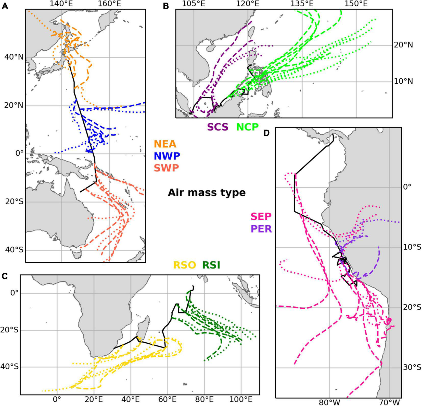
Examples illustrating the trajectories of the main air mass types found in the datasets for (A) TransBrom, (B) SHIVA, (C) OASIS, and (D) M138. Dashed lines show trajectories for arrival heights of 10 m above the ships’ positions. Dotted lines are for arrivals at 1,000 m. Examples of type EPP (M138) are not shown, as this classification was a mixture of the SEP and PER types.
Major Ions Composition in Aerosols
The chemical composition of aerosols drives aqueous and heterogeneous reactions that are important to the iodine chemistry and speciation. Coarse mode aerosols (>1 μm) in the datasets presented here are dominated by sea salt aerosols, formed through primary aerosol production mechanisms, such as sea spray and bubble bursting (Smith et al., 1993). The nss-Ca2+ concentrations in the samples reported here were extremely low, i.e., 1–2 orders of magnitude lower than reported for aerosols containing Saharan dust over the Atlantic Ocean (Baker and Yodle, 2021a). Mineral dust therefore appears to be a minor component of the TransBrom, SHIVA, OASIS, and M138 aerosols. Secondary aerosol production mechanisms, such as the oxidation and subsequent condensation of gases, are often associated with fine mode aerosol particles (<1 μm; Blanchard and Woodcock, 1980). Ions such as nss-SO42–, oxalate, and MSA are indeed predominantly found in the fine mode aerosol samples (Figure 3). NO3– has its highest concentrations in the coarse mode fractions, which is a result of nitric acid displacing Cl– within sea salt aerosols (Robbins et al., 1959; Mamane and Gottlieb, 1992; Andreae and Crutzen, 1997).
FIGURE 3
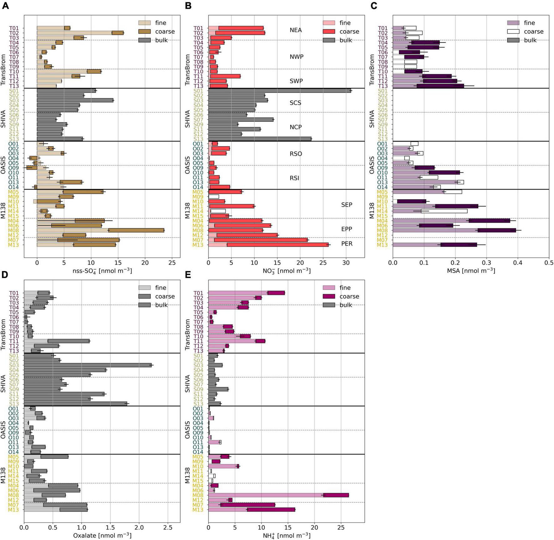
Bar plots of (A) nss-SO42–, (B) NO3–, (C) MSA, (D) oxalate, and (E) NH4+ in fine (light), coarse (dark), and bulk (grey) mode aerosol fractions for all samples of TransBrom (T01-T13), SHIVA (S01-S13), OASIS (O01-O14), and M138 (M04-M15). MSA was not measured in the SHIVA samples. Empty bars indicate concentrations below the detection limit. Nss-concentrations for which the error is larger than the parameter itself are omitted. Note that for M138 the sample order has been changed to allow the SEP, EPP, and PER air masses to be grouped together.
Notable variability in major ion concentrations indicate the influence of different natural and anthropogenic emissions in the sampled air masses. Nss-SO42–, NO3–, and oxalate are associated with fossil fuel and biomass combustion emissions. The concentrations of these ions in the aerosol samples are elevated in samples collected from air masses which have travelled over land at some point in the 5 days prior to sampling (types NEA, SCS, NCP, PER, and EPP). Similarly, NH4+, a tracer for agricultural emissions, has elevated concentrations in NEA, PER, and EPP air masses. For the SCS and NCP aerosols, NH4+ concentrations are relatively low, suggesting that these samples are primarily affected by fossil fuel combustion (Yodle and Baker, 2019). Nss-SO42– and oxalate concentrations for SWP samples, as well as some for SEP samples, are also relatively high. Relatively high MSA concentrations in maritime southern hemisphere air masses (SWP and SEP) are indicative of a marine biogenic source of dimethyl sulfide, which likely also contributes to the nss-SO42– observed in these air masses. The organic (oxalate) content of the PER and EPP air masses may carry additional strong influences of the biologically productive Peruvian coastline, known to be an upwelling region (Kamykowski and Zentara, 1990; Ulloa and Pantoja, 2009), in addition to terrestrial anthropogenic and biogenic organic matter emissions. RSO, RSI, and NWP aerosols share a similar major ion profile. Their low concentrations of nss-SO42–, NO3–, and oxalate suggest minor influence from land-based anthropogenic activities, which is consistent with their prevalent trajectories over open remote oceans. In this sense, these air masses are considered to be relatively “clean.”
Iodine Concentration and Speciation
Gas-to-particle conversion processes are the dominant source of iodine in marine aerosols (Saiz-Lopez et al., 2012a), as is quantified by the enrichment factor (EF). The EFTSI values for samples reported here range between 9 and 12,800 (Tables 4, 5). Highest TSI concentrations are found for the East Pacific Ocean aerosol samples (Figure 4 and Supplementary Figure 5), with medians ranging between 30.6 and 39.8 pmol m–3 (SEP, PER, and EPP types, fine and coarse modes combined; Supplementary Table 2). Their median EFTSI values range between 360 and 640 (Supplementary Table 2).
TABLE 4
| Cruise |
TransBrom |
SHIVA |
OASIS |
M138 |
| Species | Bulk | Bulk | Bulk | Bulk |
| TSI | 9.57 (3.08–32.0) | 9.04 (7.0–15.9) | 19.0 (12.4–30.6) | 35.6 (6.41–65.4) |
| I– | 3.66 (1.08–18.7) | 3.7 (2.25–6.09) | 4.43 (1.65–7.51) | 13.3 (1.0–33.9) |
| IO3– | 0.71 (0.35–15.0) | 4.19 (1.39–9.79) | 11.1 (5.03–18.3) | 14.7 (1.95–47.3) |
| SOI | 4.0 (−1.11–12.6) | 1.84 (−0.668–5.35) | 4.21 (2.37–7.85) | 6.4 (1.7–13.6) |
| EFTSI | 75 (16–440) | 120 (35–310) | 97 (57–280) | 470 (61–760) |
Median and range of soluble iodine species concentrations (pmol m–3) and enrichment factor (EF) of TSI in bulk aerosols for SHIVA and total (fine + coarse) for TransBrom, OASIS, and M138.
TABLE 5
| Cruise |
TransBrom |
OASIS |
M138 |
|||
| Species | Fine | Coarse | Fine | Coarse | Fine | Coarse |
| TSI | 2.86 (1.53–5.98) | 6.89 (1.55–26.7) | 8.52 (4.45–14.6) | 10.1 (4.05–16.7) | 9.59 (< 2.14–18.1) | 23.7 (4.27–58.2) |
| I– | 1.2 (0.798–2.47) | 2.27 (< 0.21–17.3) | 2.61 (1.17–5.08) | 1.44 (0.487–2.43) | 6.91 (< 0.397–14.2) | 5.55 (0.60–23.4) |
| IO3– | 0.20 (< 0.18–0.35) | 0.51 (0.13–14.8) | 3.39 (1.47–8.0) | 7.66 (2.6–11.6) | 0.72 (< 0.18–11.4) | 14.3 (1.73–45.4) |
| SOI | 1.27 (0.53–4.42) | 2.29 (−2.26–9.03) | 2.72 (1.23–4.7) | 1.54 (0.3–3.52) | 1.6 (0.795–3.72) | 3.92 (0.82–10.1) |
| EFTSI | 820 (180–3,040) | 45 (9–380) | 430 (350–1,130) | 58 (21–160) | 1,910 (440–12,800) | 330 (43–580) |
Median and range of soluble iodine species concentrations (pmol m–3) and enrichment factor (EF) of TSI in fine and coarse mode aerosols the TransBrom, OASIS, and M138 expeditions.
FIGURE 4
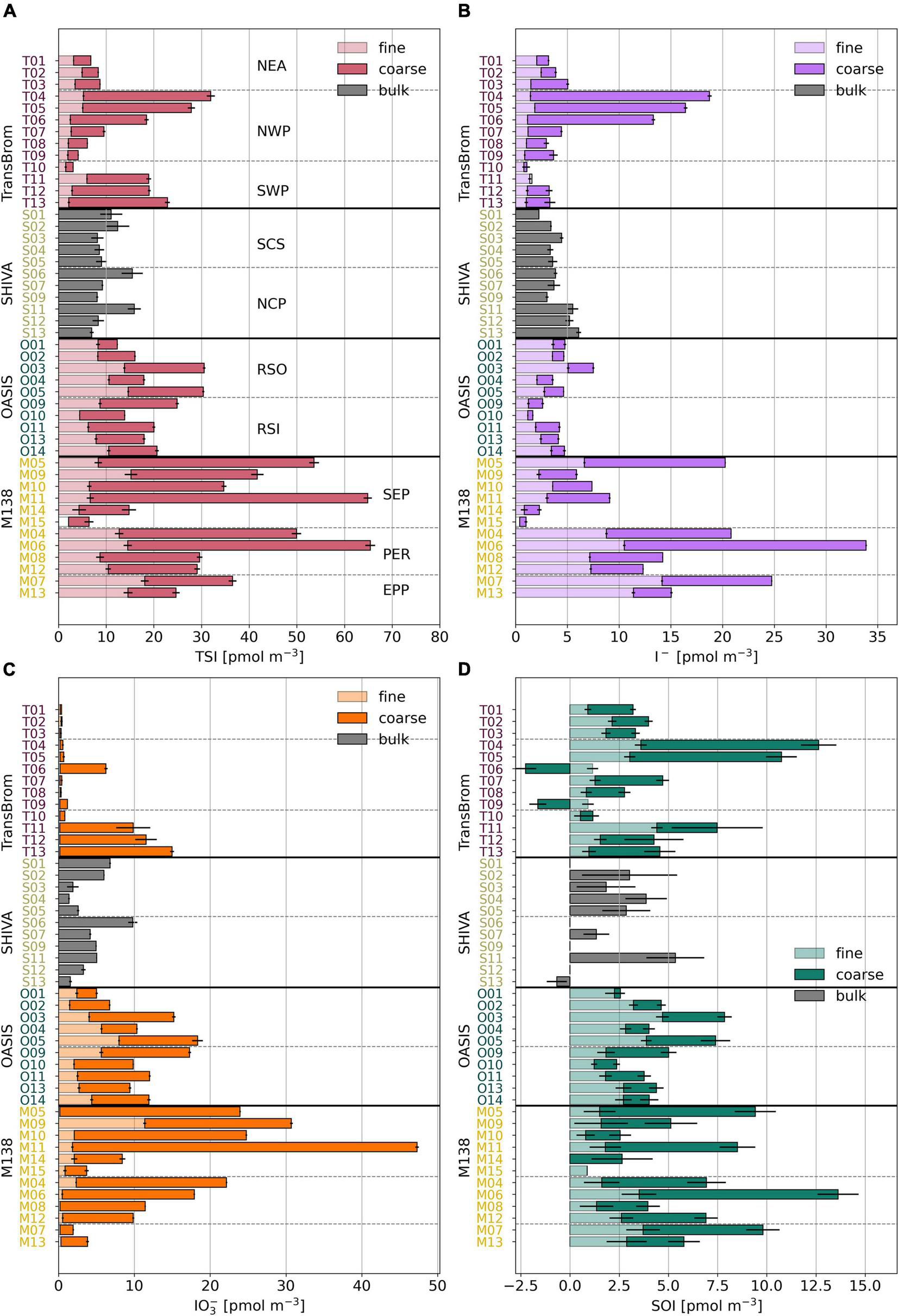
Bar plots of TSI (A), I–(B), IO3–(C), and SOI (D) concentrations in fine (light), coarse (dark), and bulk (grey) mode for TransBrom, OASIS, M138, and SHIVA aerosol samples. Empty bars indicate concentrations below the detection limit. SOI concentrations for which the error is larger than the parameter itself are omitted. Details are as for Figure 3.
The proportions of IO3–, I–, and SOI are variable within and between air mass types. Conspicuous among all samples are the low or undetectable IO3– concentrations for many of the TransBrom aerosols (West Pacific Ocean). Exceptions are the coarse mode samples T06 and T11-T13 (the three southern-most samples), which have IO3– concentrations > 9.7 pmol m–3 (Figure 4). I– and SOI are the dominant species in NEA and NWP samples, both accounting for around 50% of TSI. The coarse mode of samples T11-T13 are the only three TransBrom samples for which IO3– is the dominant species.
The bulk aerosols collected from the SCS and NCP air masses (SHIVA, West Pacific Ocean) have variable iodine species proportions where IO3– holds the highest fraction in eight of the 11 samples (Yodle and Baker, 2019). I– concentrations are relatively constant along the SHIVA track at an average of 4.0 ± 1.1 pmol m–3, although the SCS air masses seems to hold slightly less I– compared to NCP air masses (Yodle and Baker, 2019). IO3– concentrations vary between 1.4 and 9.8 pmol m–3 and are not very different between the two air mass types.
Both the fine and coarse modes of the RSO and RSI aerosol samples (OASIS, Indian Ocean) have substantial amounts of IO3– (median of 4.1/5.3 pmol m–3 in fine/coarse mode of RSO and 2.7/7.8 in fine/coarse mode of RSI). IO3– is proportionally the dominant species in the coarse mode and most of the fine mode samples. The I– concentrations in the fine mode of RSO aerosols are slightly higher (median 3.6 pmol m–3) than their coarse mode counterparts, as well as compared to the fine and coarse modes of the RSI samples (medians ranging between 1.4–1.9 pmol m–3; Supplementary Table 2).
Similarly to RSO and RSI, IO3– dominates the iodine speciation in the SEP air mass (Figure 4 and Supplementary Figure 5), although the TSI concentration for SEP is substantially higher in the coarse mode (median 27.4 pmol m–3) than in RSO and RSI (median 7.8 and 10.1 pmol m–3, respectively; Supplementary Table 2). In contrast, I– dominates the speciation for PER in both modes. EPP samples are those that are influenced by air masses of both marine and terrestrial origin, as indicated by their intermediate iodine speciation and species proportions, relative to SEP and PER (Figure 5).
FIGURE 5
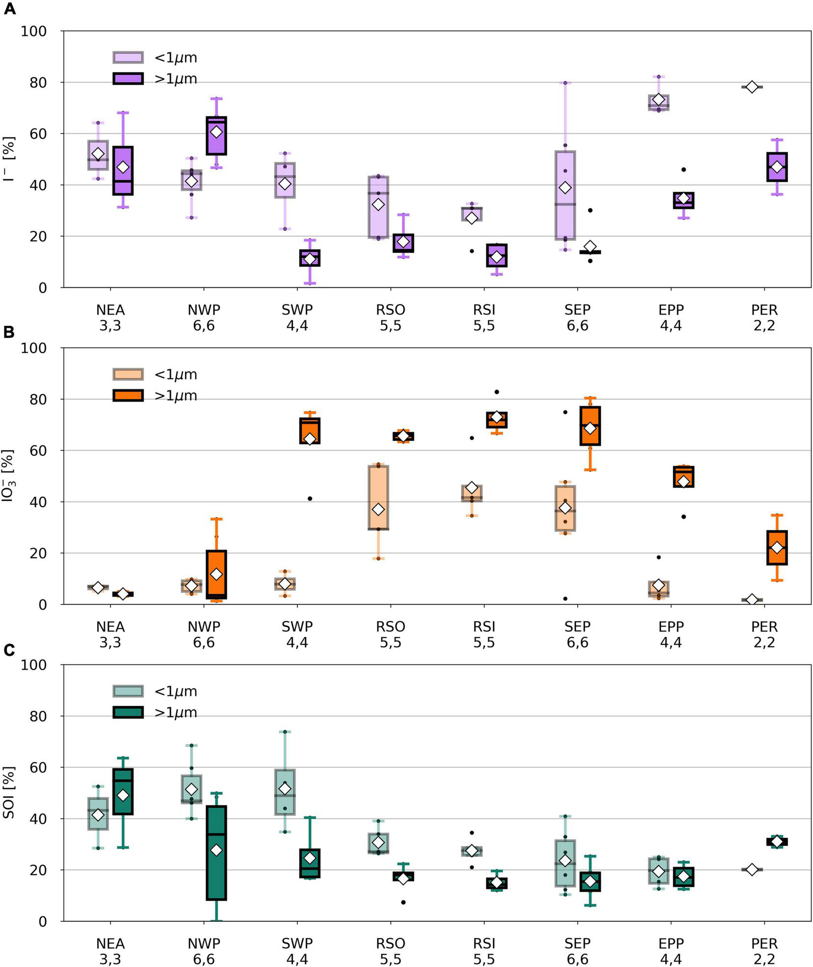
Percentage I–(A), IO3–(B), and SOI (C) of TSI in fine (light) and coarse (dark) mode aerosol samples per air mass type from TransBrom, OASIS, and M138. SOI concentrations for which the error is larger than the parameter itself are omitted. Black dots represent individual samples. White diamonds show the average value. Lower (upper) whisker extends to the sample that is within 1.5 × interquartile range lower (higher) beyond the first (third) quartile.
Except for bulk aerosol samples S12 and S13 from NCP and coarse mode aerosols T06 and T09 from NWP, SOI is found in all samples: up to 4.7 pmol m–3 in the fine mode and 10.1 pmol m–3 in the coarse mode. Consistent with previous observations in the Atlantic Ocean (Baker, 2005; Baker and Yodle, 2021a), the SOI fraction in the fine mode samples is generally larger (median 29%) than in the coarse mode samples (median 19%). In many of the TransBrom samples, SOI has higher proportions than both I– and IO3–, which has occasionally previously been observed in coastal regions (Gilfedder et al., 2008) and in the southwestern Pacific Ocean (Lai et al., 2008).
The multi-size fractionated sample from OASIS (O10) has lowest TSI concentrations in modal size fractions 0.4 and >12 μm (Figure 6). SOI is found only in modal size fractions with sizes close to 1 or <0.1 μm. Among these, its concentration ranges between 0.49 and 0.60 pmol m–3. The I– to IO3– ratio is > 1 in the two smallest modal size fractions and <1 for larger aerosol particles. The distributions of Na+, nss-SO42–, and NO3– in sample O10 are shown in Supplementary Figure 4.
FIGURE 6
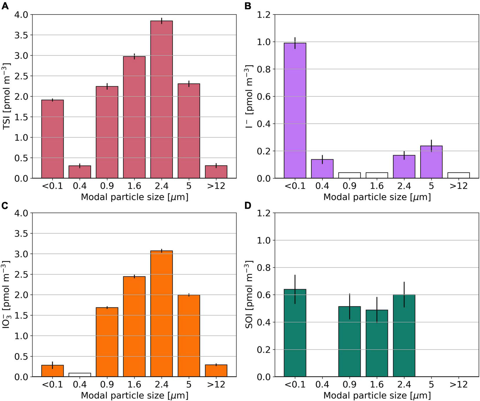
Bar plots showing the TSI (A), I–(B), IO3–(C), and SOI (D) concentrations for the multi size segregated aerosol sample O10, collected during the OASIS expedition. Empty bars indicate concentrations below the detection limit. SOI concentrations for which the error is larger than the parameter itself are omitted.
Discussion
Influences on Iodine Concentration and Speciation
Table 6 shows the bulk/total TSI concentrations and EFTSI values for the TransBrom, SHIVA, OASIS and M138 cruises, together with values reported for marine aerosols from other studies. Of the cruises reported here, TSI concentrations were highest in the M138 aerosols (particularly in the SEP samples collected off the coast of Peru; Figure 4). This may be due to stronger marine iodine sources in the eastern South Pacific. The median seawater I– concentration in this region (396 nM) is over four times higher than the global median (89.0 nM; Chance et al., 2019a,b; Supplementary Figure 7). These high surface sea water I– concentrations are probably sustained by a regional upwelling system which supplies both high I– waters [due to reduction of IO3– in the sub-surface oxygen minimum zone associated with the upwelling (Cutter et al., 2018)] and nutrient-rich waters to the surface (Ulloa and Pantoja, 2009). Enhanced phytoplankton growth driven by this nutrient supply may also lead to further reduction of IO3– to I– in surface waters (Bluhm et al., 2010). The unusually high surface I– concentrations presumably enhance the flux of volatile iodine gases to the atmosphere following dry deposition of ozone (Ganzeveld et al., 2009) and subsequent reaction of I– with ozone (Carpenter et al., 2013). Samples M14 and M15 are the most northern samples collected during the M138 campaign and are further removed from the coastal and upwelling region. This may explain the lower TSI concentrations compared to the other samples collected along the Peruvian coast. More generally, most of the results in Table 6 (with the notable exception of those from TransBrom) indicate higher TSI concentrations in the northern hemisphere than in the south. As noted by Baker and Yodle (2021a), this pattern may be a consequence of higher sea-to-air fluxes of iodine in the northern hemisphere, driven by higher ozone concentrations, and thus dry ozone deposition, in the north.
TABLE 6
| Ocean | TSI (pmol m–3) | EFTSI | References |
| Northern West Pacific | 8.7 (4.1–32.0) | 110 (16–440) | This work (TransBrom) |
| Southern West Pacific | 19.0 (3.1–22.9) | 56 (25–79) | This work (TransBrom) |
| Northern West Pacific | 9.0 (7.0–15.9) | 120 (35–310) | This work (SHIVA) |
| Southern Indian | 19.0 (12.4–30.6) | 97 (57–280) | This work (OASIS) |
| Southern East Pacific | 35.6 (6.4–65.4) | 470 (61–760) | This work (M138) |
| North Atlantic | 27.3 (13.4–91.5) | 277 (79–2,400) | Baker, 2005 |
| South Atlantic | 14.4 (8.4–32.9) | 135 (40–520) | Baker, 2005 |
| Western Pacific, Eastern Indian and Southern Ocean | 9.4* (1.2–28.2) a | Lai et al., 2008 | |
| North Atlantic | 37.5 (16.5–86.9) | 150 (100–530) | Allan et al., 2009 |
| West Pacific (30–65°N) | 82* (19–243) | Xu S. et al., 2010 | |
| South Atlantic | 5.8* (2.9–9.9) a | Lai et al., 2011 | |
| North Atlantic | 34.6 (18.6–103) | 300 (190–1,200) | Baker and Yodle, 2021a |
| South Atlantic | 21.3 (12.4–41.7) | 130 (59–620) | Baker and Yodle, 2021a |
Reported total soluble iodine (TSI) concentrations and enrichment factors of TSI with respect to sea spray in bulk/total aerosols collected over the oceans.
Values quoted are medians with ranges in parentheses, except where only means are available (*).
aPM2.5 samples were collected.
TSI concentrations in the TransBrom samples (Table 6) are comparable to those presented for aerosols < 2.5 μm (PM2.5) collected along the transect of Lai et al. (2008), which covers a similar part of the West Pacific region. The unusually low (in the context of the SHIVA, OASIS, and M138 results) IO3– concentrations observed during TransBrom are similar to those reported by Lai et al. (2008). Cellulose filters were used for sampling during TransBrom and the Lai et al. study. Yodle and Baker (2019) reported low extraction recoveries of IO3– from cellulose filters, which raises the possibility that the low IO3– proportions reported for these two cruises in the West Pacific were due to artefacts introduced by the sampling/extraction procedures. However, such an artefact (if present at all) does not appear to have affected all of the TransBrom samples, because several exhibited both high concentrations and proportions of IO3– (Figure 4C). Despite the methodological differences of TransBrom and Lai et al.’s work compared to OASIS, SHIVA, and M138, it is not clear whether the iodine speciation for these two West Pacific cruises falls outside the natural variability in iodine speciation.
Iodine Species Proportions
Iodine speciation and proportions in the RSO, RSI, and SEP (and coarse mode SWP) samples are similar to one another (Figure 5) and are comparable to those of aerosols sampled from remote marine air masses in the northern and southern Atlantic Ocean [air masses RNA and RSA in Baker (2005) and Baker and Yodle (2021a)]. Common features of these marine air masses are the dominance of IO3– in the coarse mode and high percentages of IO3– in the fine mode. This suggests that the aerosol chemistry in remote air masses across different ocean basins is governed by similar processes. The NWP samples has a radically different speciation to the other remote air mass types. As discussed above, the reasons for this difference are unclear.
Iodine species proportions in air mass types with terrestrial origins (e.g., NEA, PER) are rather different to the clean marine samples (Figure 5), with substantially lower proportions of IO3– and higher proportions of I– and SOI, especially in the fine mode. Indeed, there appears to be a gradient in the proportions of IO3– and I– in samples from continentally/anthropogenically-influenced air masses (e.g., NEA, SCS, NCP, PER, EPP) and those of clean remote air masses (e.g., RSO, RSI, SEP, SWP) (Figure 7). This is consistent with data from the Atlantic Ocean, where IO3– proportions were lower and I– and SOI proportions were higher in aerosols in air masses originating over Europe or southern Africa compared to those derived from the remote Atlantic Ocean (Baker and Yodle, 2021a).
FIGURE 7
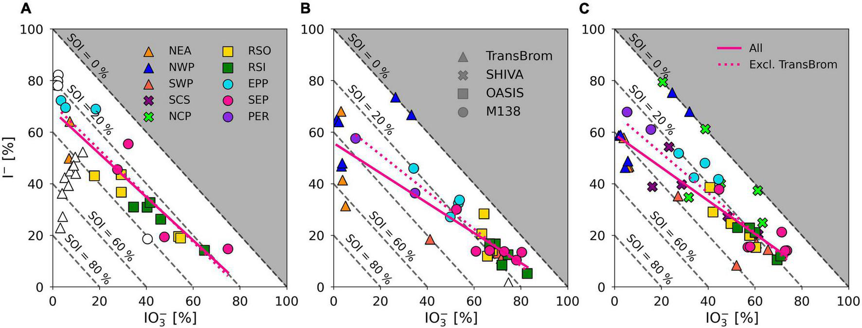
Percentage I– and IO3– of TSI plotted against each other for fine mode (A) and coarse mode (B), aerosol samples on the TransBrom, OASIS, and M138 expeditions, and bulk/total (C) aerosol samples collected on the TransBrom (triangles), OASIS (squares), M138 (circles), and SHIVA (crosses) expeditions. Colour of markers corresponds to the air mass type associated to the sample (also see Figure 2). Empty markers indicate samples for which I– or IO3– concentrations were below the detection limit. Linear regression lines are plotted for all fine, coarse, or bulk/total samples (solid) and all samples excluding those from the TransBrom expedition (dotted). Dashed diagonal lines indicate percentage of SOI of TSI. Samples for which concentrations were below the detection limit and samples where SOI < 0 are excluded from the linear regressions.
With the exception of TransBrom results, the proportion of SOI among all fine and coarse mode samples is relatively constant regardless of I– and IO3– proportions and air mass type. SOI proportions (excluding the TransBrom samples) range between 10% and 41% (median of 26 %) for fine mode samples and between 6% and 33% (median of 17%) for coarse mode samples. The higher enrichment of SOI in fine mode compared to coarse mode samples may be a result of sea spray production through bubble-bursting whereby proportionally more organic matter in the sea surface microlayer (SML) ends up in submicron film droplets rather than in the larger droplets (de Leeuw et al., 2011). If SOI is part of the composition of the organic matter, then this is a primary production mechanism. Alternatively, the organic matter may produce SOI within the aerosol through reactions with inorganic iodine compounds (Baker, 2005). In the coarse mode aerosols, SOI proportions seem lower in the remote ocean samples compared to the more continentally-influenced air masses, which could indicate primary sources of terrestrial organic matter, or primary sources of marine SOI through bubble-bursting within productive coastal regions (Seto and Duce, 1972; de Leeuw et al., 2011).
Interconversions Between Iodine Species
Baker and Yodle (2021a) recently examined the iodine speciation in aerosols collected from a variety of air mass types over the North and South Atlantic Oceans. They reported variations in speciation between these air mass types that were consistent with the controlling role of acidity on iodine species interconversions proposed by Pechtl et al. (2007). Specifically, Baker and Yodle (2021a) reported that IO3– was the dominant species in aerosols that were expected to be alkaline (i.e., unpolluted sea spray and mineral dust) and that IO3– was present in much lower proportions in aerosols that were expected to be acidic, such as in the fine mode in polluted terrestrial air masses. According to Pechtl et al. (2007), reduction of IO3– is promoted in acidic aerosols in the presence of I– (Eq. 4). Furthermore, HOI can potentially react with dissolved organic matter (DOM; Truesdale and Luther, 1995), generating SOI, which then photo-dissociates, producing I– (Baker, 2005; Eq. 5).
The variations in iodine species proportions for the samples reported here are also broadly consistent with the results of the Pechtl et al. modelling study. Clean marine aerosols (RSO, RSI, SEP) are dominated by IO3–, even in the fine mode, while the fine mode aerosols of terrestrially-influenced air mass types (NEA, PER) contain very little IO3–. These terrestrial fine mode aerosols contain relatively high concentrations of acidic species (Figure 3 and Supplementary Figure 3) and are likely to be strongly acidic (Keene et al., 2002; Pye et al., 2020). Note, however, that it was not possible to determine the pH of the samples collected during this study.
The sources and transformations of SOI in marine aerosols are still understood very poorly. In addition to the potential secondary formation of SOI (Eq. 5), it is also possible that SOI has a primary source through the direct incorporation of dissolved organic iodine (DOI) compounds into sea spray aerosols during bubble-bursting, especially for fine mode aerosols (Seto and Duce, 1972; de Leeuw et al., 2011). DOI distributions in the SML are not well known, but DOI concentrations have been reported to be higher in coastal waters than in the open ocean (Wong and Cheng, 1998). However, there does not appear to be any clear relationship between aerosol SOI concentrations or proportions and proximity of sampling locations to the coast which might indicate whether primary emissions of SOI are important.
Whether SOI has a primary or secondary source has important implications for iodine heterogeneous chemistry, because HOI also participates in other reactions, such as halogen activation that recycle I– and other halogens back to the gas-phase (Eq. 6). Therefore, secondary formation of SOI (Eq. 5) might be expected to reduce halogen recycling through competition for HOI.
However it is produced, the photodissociation of SOI is very likely to be a source of I– in aerosols. We found significant (p < 0.01) positive correlations between SOI and I– for: fine and coarse mode aerosols from M138 (R2 = 0.64, 0.77, respectively), fine mode aerosols from OASIS (R2 = 0.64), and the coarse mode aerosols from TransBrom (R2 = 0.92) (Figure 8). Positive correlations between SOI and I– concentrations have also been found for Pacific samples in other datasets (Lai et al., 2008).
FIGURE 8
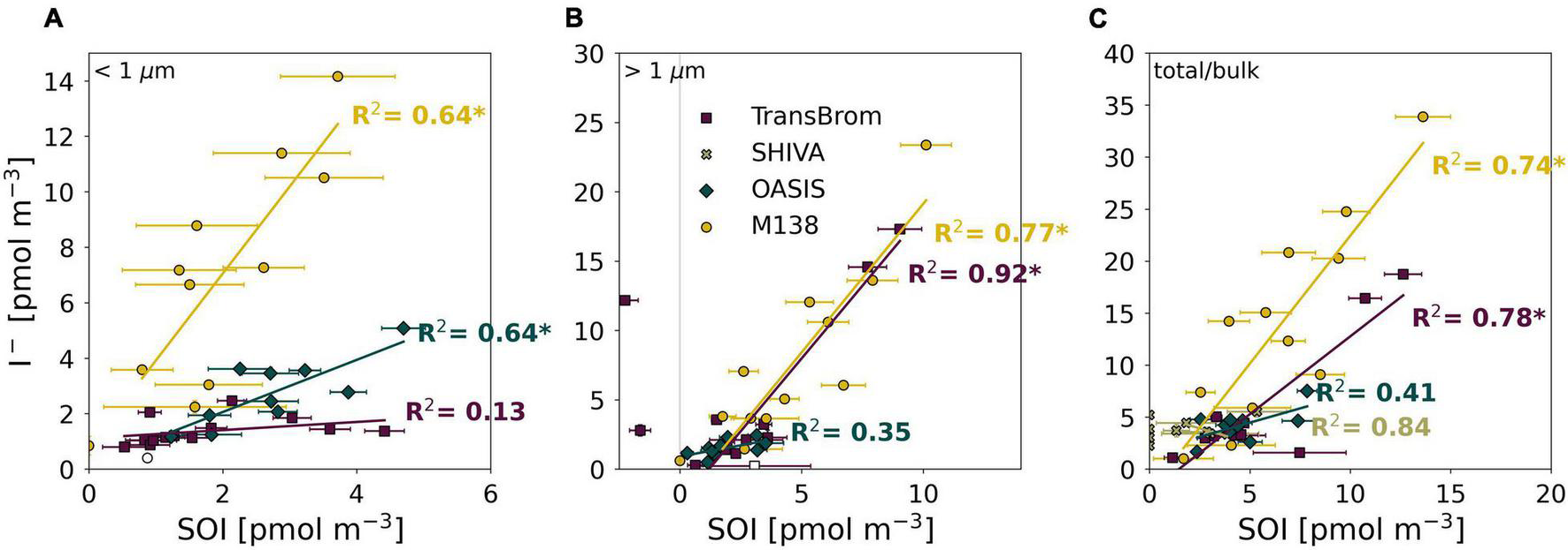
SOI and I– concentrations plotted against each other for the fine (A), coarse (B), and bulk/total mode (C) aerosol samples of TransBrom (purple), SHIVA (light green), OASIS (blue-green), and M138 (yellow). Empty markers indicate samples where the I– concentration was below detection limit. The two coarse mode samples with negative SOI concentrations for TransBrom have been excluded from linear regressions. R-squared value of each regression line are shown in the plot. * indicates a significant linear relationship p < 0.01.
The relationships between SOI and I– appear to vary between individual expeditions, especially in the fine mode (Figure 8). There are a number of factors that potentially influence these relationships, such as (a) the concentration and character of DOM and SOI in aerosols at each location which may be subject to location and seasonal variability, and (b) the acidity of the aerosol, which affects how fast I– can be recycled to the gas-phase once formed by photodissociation of SOI, the removal of I– and IO3– during reduction of IO3–, and potentially also the secondary formation of SOI (Truesdale and Luther, 1995).
Samples were collected in different seasons and years, during which iodine emissions and aerosol content have been shown to change (e.g., Xu S. et al., 2010; Cuevas et al., 2018). Changes in the magnitude and proportions of atmospheric pollutants over that time period could also have impacted aerosol iodine speciation. Even though samples in this work were collected between 2009 and 2017, we cannot assess the influence of long term or seasonal changes in our iodine speciation analysis or the observed variability. Aerosol samples are in themselves an integration of the time and space during which they were collected. Despite these contributing types of variability, the partitioning of aerosol samples into at least two size fractions and assessing the chemistry based on air mass types continues to give valuable information on the drivers of the aerosol iodine speciation.
Although the focus of this manuscript is on the speciation of iodine in the fine (<1 μm) and coarse (>1 μm) aerosol fractions, Figure 6 [and similar distributions of I–, IO3–, and SOI reported for a sample collected in the North Atlantic (Baker and Yodle, 2021a)] indicates that there is considerable heterogeneity of iodine speciation and the distribution of species that affect acidity (Supplementary Figure 4) within the fine and coarse fractions.
Wider Implications for Iodine Biogeochemistry
Paleoclimate research on Antarctic ice cores found detectable I– throughout a record spanning the last 215 ky, but could only detect IO3– in ice from glacial time periods with high dust fluxes (Spolaor et al., 2013). This is consistent with the association between high IO3– concentrations and mineral dust in present-day marine aerosols (Baker and Yodle, 2021a) and suggests that dust alkalinity might account for the stability of IO3– in ice cores. Baker and Yodle (2021a) suggested that pH changes in fine and coarse mode aerosols in response to changing pollutant emissions since the Industrial Revolution (Baker et al., 2021) might affect iodine cycling (and ozone destruction rates) over time. Coastal mega cities are regions where aerosols have both high concentrations of sea spray and acidic species due to pollution. The results presented here suggest that acidification of sea spray aerosols potentially has an impact on iodine activation and thus on ozone destruction in those environments.
Conclusion
The data presented here for the West Pacific Ocean, East Pacific Ocean, and Indian Ocean contribute to a growing observational dataset on aerosol iodine speciation over the global ocean. While the results show appreciable variability among air masses and aerosol size fractions, they are broadly consistent with observations recently reported for the Atlantic Ocean (Baker and Yodle, 2021a). The use of uniform sampling and analytical methods between these two studies has allowed the general patterns in aerosol iodine speciation to be identified across all the major ocean basins for the first time. In alkaline aerosols, such as clean sea spray or mineral dust aerosols, IO3– is the dominant species. In aerosols with higher acidity and I– availability, especially in polluted fine mode aerosols, IO3– is a minor species and I– and SOI make up more significant fractions of the soluble iodine. Aerosol acidity is thought to be a major factor affecting the ratio of IO3– and I– concentrations (Pechtl et al., 2007) and variations in acidity very likely contribute to the differences between iodine speciation in fine and coarse mode aerosols. SOI appears to be ubiquitous in marine aerosols. Its role in aerosol iodine cycling, and the wider impacts of iodine chemistry on tropospheric ozone, is dependent to some extent on the sources of SOI (primary or secondary, marine or terrestrial) and likely also on its composition, about which relatively little is known. Future progress in this area will require the measurement (Craig et al., 2018) or calculation (Pye et al., 2020) of aerosol pH together with iodine speciation. Better understanding of the molecular character, sources, and reactivity of SOI will be necessary in order to incorporate the influence of this iodine fraction in numerical models of aerosol chemistry.
The robustness of the chemical drivers discussed in this work need to be tested alongside physical processes by process-based models, aiming to simulate representative aerosol iodine speciation in various environmental conditions, i.e., air mass types. The tight coupling between the aqueous-phase and gas-phase chemistry requires that gas-phase species concentrations be also validated, including the effect on atmospheric ozone levels and potential oceanic ozone deposition. Models can also address the combined effect of the aerosol iodine chemistry on marine ozone deposition and possible feedback processes through oceanic iodine emission and subsequent ozone destruction pathways. The globally consistent observational datasets presented here and by Baker and Yodle (2021a), together with the global sea surface I– observations (Chance et al., 2019a), provide a significant benchmark to support those process modelling studies.
Publisher’s Note
All claims expressed in this article are solely those of the authors and do not necessarily represent those of their affiliated organizations, or those of the publisher, the editors and the reviewers. Any product that may be evaluated in this article, or claim that may be made by its manufacturer, is not guaranteed or endorsed by the publisher.
Statements
Data availability statement
The datasets presented in this study can be found in the PANGAEA online repository at the following links: https://doi.org/10.1594/PANGAEA.935937 (TransBrom), https://doi.org/10.1594/PANGAEA.891321 (SHIVA), https://doi.org/10.1594/PANGAEA.935883 (OASIS), and https://doi.org/10.1594/PANGAEA.936483 (M138).
Author contributions
ED led the writing process of the manuscript, and analysed, processed, and interpreted the OASIS iodine species results. AB developed the concept for the study and contributed to the writing of the manuscript. CY analysed, processed, and interpreted the major ion and iodine species results for TransBrom and SHIVA. AS analysed, processed, and interpreted the major ion and iodine species concentrations for M138. LG co-guided the process of the study on the OASIS aerosol samples. All authors commented on the manuscript.
Funding
We would like to thank the Royal Thai Government for providing a studentship for CY and the United Kingdom Natural Environment Research Council (Grant NE/H00548X/1) and the University of East Anglia for supporting analysis costs. We would also like to thank the German Federal Ministry of Education and Research (BMBF) for providing the funding for the TransBrom (Grant No. 03G0731A), SHIVA (Grant No. 03G218A), and OASIS (Grant No. 03G0235A) expeditions. M138 was funded by the German Science Foundation (DFG) via the Collaborative Research Centre (Sonderforschungsbereich) 754 at Kiel University/GEOMAR, Kiel, Germany (www.sfb754.de).
Acknowledgments
We would like to thank the Peruvian authorities for their generous permission to work in their territorial waters. We would also like to thank Yuanxin Tian for measuring the major ion composition in the OASIS samples, and Graham Chilvers for assistance with the IC-ICP-MS analyses. We would also further like to thank the following people for aerosol sample collection: Christian Müller, Sebastian Wache and Arne Lanatowitz (TransBrom), Anke Schneider (SHIVA), Birgit Quack (SHIVA and OASIS), and Hermann Bange (M138). We would additionally like to thank Birgit Quack for the coordination of the sample collection on the TransBrom, SHIVA, and OASIS expeditions. We would also like to thank two reviewers for their time and valuable comments, which helped us improve the quality of the manuscript.
Conflict of interest
The authors declare that the research was conducted in the absence of any commercial or financial relationships that could be construed as a potential conflict of interest.
Supplementary material
The Supplementary Material for this article can be found online at: https://www.frontiersin.org/articles/10.3389/fmars.2021.788105/full#supplementary-material
References
1
Allan J. D. Topping D. O. Good N. Irwin M. Flynn M. Williams P. I. et al (2009). Composition and properties of atmospheric particles in the eastern Atlantic and impacts on gas phase uptake rates.Atmos. Chem. Phys.99299–9314. 10.5194/acp-9-9299-2009
2
Andreae M. O. Crutzen P. J. (1997). Atmospheric aerosols: biogeochemical sources and role in atmospheric chemistry.Science2761052–1058. 10.1126/science.276.5315.1052
3
Baker A. R. (2004). Inorganic iodine speciation in tropical Atlantic aerosol.Geophys. Res. Lett.31:L23S02. 10.1029/2004GL020144
4
Baker A. R. (2005). Marine aerosol iodine chemistry: the importance of soluble organic iodine.Environ. Chem.2295–298. 10.1071/EN05070
5
Baker A. R. (2021). Aerosol Chemical Composition (Major Ions and Iodine Species) in Samples Collected During the M138 Cruise in the Eastern Pacific Ocean, June 2017. PANGAEA. 10.1594/PANGAEA.936483
6
Baker A. R. Droste E. (2021). Aerosol Soluble Chemical Composition for OASIS Cruise (SO234/2 & SO235), Indian Ocean, July-August 2014, Determined By Ion Chromatography and Inductively Coupled Plasma - Mass Spectrometry. PANGAEA. 10.1594/PANGAEA.935883
7
Baker A. R. Kanakidou M. Nenes A. Myriokefalitakis S. Croot P. L. Duce R. A. et al (2021). Changing atmospheric acidity as a modulator of nutrient deposition and ocean biogeochemistry.Sci. Adv.7:eabd8800. 10.1126/sciadv.abd8800
8
Baker A. R. Tunnicliffe C. Jickells T. D. (2001). Iodine speciation and deposition fluxes from the marine atmosphere.J. Geophys. Res. Atmos.10628743–28749. 10.1029/2000JD000004
9
Baker A. R. Yodle C. (2018). Aerosol Major Ions and Iodine Speciation Over South China and Sulu Seas collected daily during SONNE Cruise SO218. PANGAEA. 10.1594/PANGAEA.891321
10
Baker A. R. Yodle C. (2021b). Aerosol Chemical Composition (Major Ions and Iodine Speciation) During the TransBrom Cruise in the Western Pacific Ocean, October 2009. PANGAEA. 10.1594/PANGAEA.935937
11
Baker A. R. Yodle C. (2021a). Measurement report: indirect evidence for the controlling influence of acidity on the speciation of iodine in Atlantic aerosols.Atmos. Chem. Phys.2113067–13076. 10.5194/acp-21-13067-2021
12
Bange H. Arevalo-Martinez D. L. Baker A. R. Bristow L. Burmeister K. Cisternas-Novoa C. et al (2017). Organic Matter Fluxes and Biogeochemical Processes in the OMZ Off Peru, Cruise No. M138, 01 June-03 July 2017, Callao (Peru)-Bahia Las Minas (Panama), Open Access. Meteor-Berichte, 138.Bonn: Gutachterpanel Forschungsschiffe, 69. 10.2312/cr_m138
13
Blanchard D. C. Woodcock A. H. (1980). The production, concentration, and vertical distribution of the sea-salt aerosol.Ann. N. Y. Acad. Sci.338330–347. 10.1111/j.1749-6632.1980.tb17130.x
14
Bluhm K. Croot P. Wuttig K. Lochte K. (2010). Transformation of iodate to iodide in marine phytoplankton driven by cell senescence.Aquat. Biol.111–15. 10.3354/ab00284
15
Carpenter L. J. MacDonald S. M. Shaw M. D. Kumar R. Saunders R. W. Parthipan R. et al (2013). Atmospheric iodine levels influenced by sea surface emissions of inorganic iodine.Nat. Geosci.6108–111. 10.1038/ngeo1687
16
Chameides W. L. Davis D. D. (1980). Iodine: its possible role in tropospheric photochemistry.J. Geophys. Res. Oceans857383–7398. 10.1029/JC085iC12p07383
17
Chance R. Tinel L. Sherwen T. Baker A. Bell T. Brindle J. et al (2019a). Global sea-surface iodide observations, 1967–2018.Sci. Data6:286. 10.1038/s41597-019-0288-y
18
Chance R. Tinel L. Sherwen T. Baker A. Bell T. Brindle J. et al (2019b). Global Sea-Surface Iodide Observations, 1967-2018.Swindon: Natural Environment Research Council.
19
Chatfield R. B. Crutzen P. J. (1990). Are there interactions of iodine and sulfur species in marine air photochemistry?J. Geophys. Res. Atmos.9522319–22341. 10.1029/JD095iD13p22319
20
Craig R. L. Peterson P. K. Nandy L. Lei Z. Hossain M. A. Camarena S. et al (2018). Direct determination of aerosol pH: size-resolved measurements of submicrometer and supermicrometer aqueous particles.Anal. Chem.9011232–11239. 10.1021/acs.analchem.8b00586
21
Cuevas C. A. Maffezzoli N. Corella J. P. Spolaor A. Vallelonga P. Kjær H. A. et al (2018). Rapid increase in atmospheric iodine levels in the North Atlantic since the mid-20th century.Nat. Commun.9:1452. 10.1038/s41467-018-03756-1
22
Cutter G. A. Moffett J. G. Nielsdottir M. C. Sanial V. (2018). Multiple oxidation state trace elements in suboxic waters off Peru: in situ redox processes and advective/diffusive horizontal transport.Mar. Chem.20177–89. 10.1016/j.marchem.2018.01.003
23
Davis D. Crawford J. Liu S. McKeen S. Bandy A. Thornton D. et al (1996). Potential impact of iodine on tropospheric levels of ozone and other critical oxidants.J. Geophys. Res. Atmos.1012135–2147. 10.1029/95JD02727
24
de Leeuw G. Andreas E. L. Anguelova M. D. Fairall C. W. Lewis E. R. O’Dowd C. et al (2011). Production flux of sea spray aerosol.Rev. Geophys.49:RG2001. 10.1029/2010RG000349
25
Gäbler H. E. Heumann K. G. (1993). Determination of atmospheric iodine species using a system of specifically prepared filters and IDMS.Fresenius J. Anal. Chem.34553–59. 10.1007/BF00323326
26
Ganzeveld L. Helmig D. Fairall C. W. Hare J. Pozzer A. (2009). Atmosphere-ocean ozone exchange: a global modeling study of biogeochemical, atmospheric, and waterside turbulence dependencies.Glob. Biogeochem. Cycles23:GB4021. 10.1029/2008GB003301
27
Gilfedder B. S. Lai S. C. Petri M. Biester H. Hoffmann T. (2008). Iodine speciation in rain, snow and aerosols.Atmos. Chem. Phys.86069–6084. 10.5194/acp-8-6069-2008
28
Gómez Martín J. C. Saiz-Lopez A. Cuevas C. A. Fernandez R. P. Gilfedder B. Weller R. et al (2021). Spatial and temporal variability of iodine in aerosol.J. Geophys. Res. Atmos.126:e2020JD034410. 10.1029/2020JD034410
29
Hoffmann T. O’Dowd C. D. Seinfeld J. H. (2001). Iodine oxide homogeneous nucleation: an explanation for coastal new particle production.Geophys. Res. Lett.281949–1952. 10.1029/2000GL012399
30
Jones C. E. Hornsby K. E. Sommariva R. Dunk R. M. Von Glasow R. McFiggans G. et al (2010). Quantifying the contribution of marine organic gases to atmospheric iodine.Geophys. Res. Lett.37:L18804. 10.1029/2010GL043990
31
Kamykowski D. Zentara S. J. (1990). Hypoxia in the world ocean as recorded in the historical data set.Deep Sea Res. Part A Oceanogr. Res. Papers371861–1874. 10.1016/0198-0149(90)90082-7
32
Keene W. C. Pszenny A. A. Maben J. R. Sander R. (2002). Variation of marine aerosol acidity with particle size.Geophys. Res. Lett.29:1101. 10.1029/2001GL013881
33
Klick S. Abrahamsson K. (1992). Biogenic volatile iodated hydrocarbons in the ocean.J. Geophys. Res. Oceans9712683–12687. 10.1029/92JC00948
34
Krüger K. Quack B. Marandino C. (2014a). RV SONNEFahrtbericht/Cruise Report SO234-2, 08-20.07.2014, Durban, South Africa-PortLouis, Mauritius -SPACES OASIS Indian Ocean, GEOMAR Report, N.Ser.020.Kiel: GEOMAR, 87.
35
Krüger K. Quack B. Marandino C. (2014b). RV SONNEFahrtbericht/Cruise Report SO235, 23.07-07.08.2014, PortLouis, Mauritius to Malé, Maldives, GEOMAR Report, N.Ser.021.Kiel: GEOMAR, 65.
36
Lai S. C. Hoffmann T. Xie Z. Q. (2008). Iodine speciation in marine aerosols along a 30,000 km round-trip cruise path from Shanghai, China to Prydz Bay, Antarctica.Geophys. Res. Lett.35L21803. 10.1029/2008GL035492
37
Lai S. C. Williams J. Arnold S. R. Atlas E. L. Gebhardt S. Hoffmann T. (2011). Iodine containing species in the remote marine boundary layer: a link to oceanic phytoplankton.Geophys. Res. Lett.38:L20801. 10.1029/2011GL049035
38
Mahajan A. Gómez Martín J. Hay T. Royer S.-J. Yvon-Lewis S. Liu Y. et al (2012). Latitudinal distribution of reactive iodine in the Eastern Pacific and its link to open ocean sources.Atmos. Chem. Phys.1211609–11617. 10.5194/acp-12-11609-2012
39
Mahajan A. Plane J. Oetjen H. Mendes L. Saunders R. Saiz-Lopez A. et al (2010). Measurement and modelling of tropospheric reactive halogen species over the tropical Atlantic Ocean.Atmos. Chem. Phys.104611–4624. 10.5194/acp-10-4611-2010
40
Mamane Y. Gottlieb J. (1992). Nitrate formation on sea-salt and mineral particles - a single particle approach.Atmos. Environ. Part A Gen. Top.261763–1769. 10.1016/0960-1686(92)90073-T
41
Martino M. Hamilton D. Baker A. R. Jickells T. D. Bromley T. Nojiri Y. et al (2014). Western Pacific atmospheric nutrient deposition fluxes, their impact on surface ocean productivity.Glob. Biogeochem. Cycles28712–728. 10.1002/2013GB004794
42
Martino M. Mills G. P. Woeltjen J. Liss P. S. (2009). A new source of volatile organoiodine compounds in surface seawater.Geophys. Res. Lett.36:L01609. 10.1029/2008GL036334
43
McFiggans G. Plane J. M. Allan B. J. Carpenter L. J. Coe H. O’Dowd C. (2000). A modeling study of iodine chemistry in the marine boundary layer.J. Geophys. Res. Atmos.10514371–14385. 10.1029/1999JD901187
44
Moore R. M. Tokarczyk R. (1992). Chloro-iodomethane in N. Atlantic waters: a potentially significant source of atmospheric iodine.Geophys. Res. Lett.191779–1782. 10.1029/92GL01796
45
O’Dowd C. D. Jimenez J. L. Bahreini R. Flagan R. C. Seinfeld J. H. Hämeri K. et al (2002). Marine aerosol formation from biogenic iodine emissions.Nature417632–636. 10.1038/nature00775
46
Pechtl S. Schmitz G. Glasow R. V. (2007). Modelling iodide–iodate speciation in atmospheric aerosol: contributions of inorganic and organic iodine chemistry.Atmos. Chem. Phys.71381–1393. 10.5194/acp-7-1381-2007
47
Prados-Roman C. Cuevas C. A. Fernandez R. P. Kinnison D. E. Lamarque J. F. Saiz-Lopez A. (2015a). A negative feedback between anthropogenic ozone pollution and enhanced ocean emissions of iodine.Atmos. Chem. Phys.152215–2224. 10.5194/acp-15-2215-2015
48
Prados-Roman C. Cuevas C. A. Hay T. Fernandez R. P. Mahajan A. S. Royer S. J. et al (2015b). Iodine oxide in the global marine boundary layer.Atmos. Chem. Phys.15583–593. 10.5194/acp-15-583-2015
49
Pye H. O. T. Nenes A. Alexander B. Ault A. P. Barth M. C. Clegg S. L. et al (2020). The acidity of atmospheric particles and clouds.Atmos. Chem. Phys.204809–4888. 10.5194/acp-20-4809-2020
50
Quack B. Krüger K. (2010). FS SONNE Fahrtbericht/Cruise Report: TransBrom SONNE, Tomakomai, Japan-Townsville, Australia, 09.10.-24.10.2009 [SO202-TRANSIT].Kiel: IFM-GEOMAR.
51
Quack B. Krüger K. (2013). RV SONNE Fahrtbericht/Cruise Report SO218 SHIVA 15-29.11. 2011 Singapore-Manila, Philippines stratospheric ozone: halogens in a varying atmosphere part 1: SO218-SHIVA summary report (in German) part 2: SO218-SHIVA english reports of participating groups.GEOMAR Rep. (N. Ser.)12:112.
52
Read K. A. Mahajan A. S. Carpenter L. J. Evans M. J. Faria B. V. Heard D. E. et al (2008). Extensive halogen-mediated ozone destruction over the tropical Atlantic Ocean.Nature4531232–1235. 10.1038/nature07035
53
Robbins R. C. Cadle R. D. Eckhardt D. L. (1959). The conversion of sodium chloride to hydrogen chloride in the atmosphe.J. Atmos. Sci.1653–56. 10.1175/1520-04691959016<0053:TCOSCT<2.0.CO;2
54
Saiz-Lopez A. Lamarque J. F. Kinnison D. E. Tilmes S. Ordóñez C. Orlando J. J. et al (2012b). Estimating the climate significance of halogen-driven ozone loss in the tropical marine troposphere.Atmos. Chem. Phys.123939–3949. 10.5194/acp-12-3939-2012
55
Saiz-Lopez A. Plane J. M. Baker A. R. Carpenter L. J. von Glasow R. Gómez Martín J. C. et al (2012a). Atmospheric chemistry of iodine.Chem. Rev.1121773–1804. 10.1021/cr200029u
56
Schall C. Heumann K. G. Kirst G. O. (1997). Biogenic volatile organoiodine and organobromine hydrocarbons in the Atlantic ocean from 42 N to 72 S.Fresenius J. Anal. Chem.359298–305. 10.1007/s002160050577
57
Seto F. Y. Duce R. A. (1972). A laboratory study of iodine enrichment on atmospheric sea-salt particles produced by bubbles.J. Geophys. Res.775339–5349. 10.1029/JC077i027p05339
58
Smith M. H. Park P. M. Consterdine I. E. (1993). Marine aerosol concentrations and estimated fluxes over the sea.Q. J. R. Meteorol. Soc.119809–824. 10.1002/qj.49711951211
59
Spolaor A. Vallelonga P. Plane J. M. C. Kehrwald N. Gabrieli J. Varin C. (2013). Halogen species record Antarctic sea ice extent over glacial–interglacial periods.Atmos. Chem. Phys.136623–6635. 10.5194/acp-13-6623-2013
60
Stein A. F. Draxler R. R. Rolph G. D. Stunder B. J. Cohen M. D. Ngan F. (2015). NOAA’s HYSPLIT atmospheric transport and dispersion modeling system.Bull. Am. Meteorol. Soc.962059–2077. 10.1175/BAMS-D-14-00110.1
61
Stumm W. Morgan J. J. (2012). Aquatic Chemistry: Chemical Equilibria and Rates in Natural Waters, Vol. 126. Hoboken, NJ: John Wiley & Sons.
62
Truesdale V. W. Luther G. W. (1995). Molecular iodine reduction by natural and model organic substances in seawater.Aquat. Geochem.189–104. 10.1007/BF01025232
63
Ulloa O. Pantoja S. (2009). The oxygen minimum zone of the eastern South Pacific.Deep Sea Res. Part II Top. Stud. Oceanogr.56987–991. 10.1016/j.dsr2.2008.12.004
64
Vogt R. Sander R. Von Glasow R. Crutzen P. J. (1999). Iodine chemistry and its role in halogen activation and ozone loss in the marine boundary layer: a model study.J. Atmos. Chem.32375–395. 10.1023/A:1006179901037
65
Whitehead D. C. (1984). The distribution and transformations of iodine in the environment.Environ. Int.10321–339. 10.1016/0160-4120(84)90139-9
66
Wimschneider A. Heumann K. G. (1995). Iodine speciation in size fractionated atmospheric particles by isotope dilution mass spectrometry.Fresenius J. Anal. Chem.353191–196. 10.1007/s0021653530191
67
Wong G. T. (1991). The marine geochemistry of iodine.Rev. Aquat. Sci.445–73.
68
Wong G. T. Cheng X. H. (1998). Dissolved organic iodine in marine waters: determination, occurrence and analytical implications.Mar. Chem.59271–281. 10.1016/S0304-4203(97)00078-9
69
Xu S. Xie Z. Li B. Liu W. Sun L. Kang H. et al (2010). Iodine speciation in marine aerosols along a 15 000-km round-trip cruise path from Shanghai, China, to the Arctic Ocean.Environ. Chem.7406–412. 10.1071/EN10048
70
Xu S.-Q. Xie Z.-Q. Liu W. Yang H.-X. Li B. (2010). Extraction and determination of total bromine, iodine, and their species in atmospheric aerosol.Chin. J. Anal. Chem.38219–224. 10.1016/S1872-2040(09)60026-8
71
Yodle C. Baker A. R. (2019). Influence of collection substrate and extraction method on the speciation of soluble iodine in atmospheric aerosols.Atmos. Environ. X1:100009. 10.1016/j.aeaoa.2019.100009
Summary
Keywords
iodine speciation, marine aerosols, Indian Ocean, Pacific Ocean, marine boundary layer (MBL)
Citation
Droste ES, Baker AR, Yodle C, Smith A and Ganzeveld L (2021) Soluble Iodine Speciation in Marine Aerosols Across the Indian and Pacific Ocean Basins. Front. Mar. Sci. 8:788105. doi: 10.3389/fmars.2021.788105
Received
01 October 2021
Accepted
17 November 2021
Published
09 December 2021
Volume
8 - 2021
Edited by
Anoop Sharad Mahajan, Indian Institute of Tropical Meteorology (IITM), India
Reviewed by
Andrea Spolaor, National Research Council, Consiglio Nazionale delle Ricerche (CNR), Italy; Manuel Dall’Osto, Institute of Marine Sciences, Spanish National Research Council (CSIC), Spain
Updates
Copyright
© 2021 Droste, Baker, Yodle, Smith and Ganzeveld.
This is an open-access article distributed under the terms of the Creative Commons Attribution License (CC BY). The use, distribution or reproduction in other forums is permitted, provided the original author(s) and the copyright owner(s) are credited and that the original publication in this journal is cited, in accordance with accepted academic practice. No use, distribution or reproduction is permitted which does not comply with these terms.
*Correspondence: Elise S. Droste, e.droste@uea.ac.uk
†Present address: Chan Yodle, Department of Environmental Science, Faculty of Science and Technology, Chiang Mai Rajabhat University, Chiang Mai, Thailand
This article was submitted to Marine Biogeochemistry, a section of the journal Frontiers in Marine Science
Disclaimer
All claims expressed in this article are solely those of the authors and do not necessarily represent those of their affiliated organizations, or those of the publisher, the editors and the reviewers. Any product that may be evaluated in this article or claim that may be made by its manufacturer is not guaranteed or endorsed by the publisher.