Abstract
During recent years, experimental ecology started to focus on regional to local environmental fluctuations in the context of global climate change. Among these, marine heatwaves can pose significant threats to marine organisms. Yet, experimental studies that include fluctuating thermal stress are rare, and if available often fail to base experimental treatments on available long-term environmental data. We evaluated 22-year high-resolution sea surface temperature data on the occurrence of heatwaves and cold-spells in a temperate coastal marine environment. The absence of a general warming trend in the data may in parts be responsible for a lack of changes in heatwave occurrences (frequency) and their traits (intensity, duration, and rate of change) over time. Yet, the retrieved traits for present-day heatwaves ensured most-natural treatment scenarios, enabling an experimental examination of the impacts of marine heatwaves and phases of recovery on an important temperate predator, the common sea star Asterias rubens. In a 68-days long experiment, we compared a 37- and a 28-days long heatwave with a treatment that consisted of three consecutive 12-days long heatwaves with 4 days of recovery in between. The heatwaves had an intensity of 4.6°C above climatological records, resulting in a maximum temperature of 23.25°C. We demonstrate that heatwaves decrease feeding and activity of A. rubens, with longer heatwaves having a more severe and lasting impact on overall feeding pressure (up to 99.7% decrease in feeding rate) and growth (up to 87% reduction in growth rate). Furthermore, heatwaves of similar overall mean temperature, but interrupted, had a minor impact compared to continuous heatwaves, and the impact diminished with repeated heatwave events. We experimentally demonstrated that mild heatwaves of today’s strength decrease the performance of A. rubens. However, this echinoderm may use naturally occurring short interruptions of thermal stress as recovery to persist in a changing and variable ocean. Thus, our results emphasize the significance of thermal fluctuations and especially, the succession and timing of heat-stress events.
Introduction
Anthropogenically induced climate change alters the abiotic conditions for all marine organisms and ecosystems (IPCC, 2021). Thereby, sea surface temperatures (SSTs) are projected to increase by 3°C until the end of this century (IPCC, 2021), which has been shown to negatively impact ecosystems worldwide (Walther et al., 2002; Doney et al., 2012; IPCC, 2021).
Thermal fluctuations are superimposed on this gradual change in temperature, reaching from yearly (seasonal) to daily (day-night) or tidal fluctuations. While colder periods may serve as refuge from heat stress in a fluctuating world, peak temperatures cause high thermal stress temporally (Wahl et al., 2015). Therefore, the examination of natural fluctuations and their extremes is key to understand a system’s response to a warming ocean. Among the most important thermal fluctuations, heatwave events are projected to increase in frequency, duration, and intensity worldwide (Oliver et al., 2018), with particular intensification in marginal shallow seas, like the Baltic Sea (Gräwe et al., 2013).
Heatwaves have a high potential of impacting marine ecosystems, by exceeding the thermal limits of species (Oliver et al., 2019; Smale et al., 2019). Much research has been done in tropical systems such as coral reefs, as slight temperature deviations can have massive impacts leading to, e.g., coral bleaching (Le Nohaïc et al., 2017). In coral reef ecosystems, the accumulation of thermal anomalies is used to assess the bleaching potential (degree heating weeks; e.g., Kayanne, 2017). The impact of temperature events on marine ecosystems therefore depends on a heatwave’s intensity, but also on traits such as duration (e.g., Oliver et al., 2019) and onset rates (e.g., Genin et al., 2020). Thus, even in temperate regions, with generally higher thermal variability, heatwaves can have strong impacts on marine ecosystems (Pansch et al., 2018; Smale et al., 2019), yet the overall effect strength and direction may strongly depend on the timing of the heatwave event and on the environmental history of the community (Pansch et al., 2018).
Generally, acclimation to environmental change may occur across species, challenging reliable predictions of future ecosystem changes. As shown for multiple simultaneous drivers (Boyd et al., 2018), consecutive stress events (e.g., recurring marine heatwaves) can either have additive, antagonistic or synergistic impacts on species (Gunderson et al., 2016). Antagonistic impacts can mean that a first stressor prepares the organism to respond more adequately when the same stressor recurs, a concept referred to as “stress memory” or “ecological memory” (e.g., Walter et al., 2013; Jackson et al., 2021). At the species level, such processes are triggered by, for example, the expression of heat shock proteins (HSPs, e.g., Todgham et al., 2005; Banti et al., 2008; McBryan et al., 2016), while at the population and the community level, genotype, and species sorting as well as changes in dispersal capacities or species interactions can trigger such “lagged” effects, long after a stress event occurred [as discussed by Jackson et al. (2021)].
Environmental climate change has the potential to drive ecosystem responses if keystone species are impacted (Sanford, 1999). The common sea star (Asterias rubens) is such a keystone species in the temperate benthic communities of the Atlantic Ocean, North Sea and Baltic Sea (Vevers, 1949; Budd, 2008). This species is an important part of the ecosystem as it controls the abundance of mussels and thus, the distribution of mussel beds (Gaymer et al., 2001). Mussels, e.g., blue mussels, (Mytilus spp.) play an important role as ecosystem engineers by providing habitat for many other species (Norling and Kautsky, 2007; Sadchatheeswaran et al., 2015). Yet, when released from one of their main predators, mussels might outcompete other important structure-forming species like seagrasses and macroalgae by forming large monocultures and thus decreasing overall diversity (Reusch and Chapman, 1997; Dürr and Wahl, 2004).
Even though the importance of environmental variability, including marine heatwaves, is widely acknowledged in the scientific community (Pincebourde et al., 2012; Gunderson et al., 2016; Smale et al., 2019), this aspect is often neglected in experimental ecology. One major problem may be the lack of a universal characterization of variability such as marine heatwave events. In this study, we used a physical (oceanographic) approach suggested by Hobday et al. (2016), which is now widely used in characterizing marine heatwave events globally (Oliver et al., 2019; Smale et al., 2019; Thomsen et al., 2019), thus allowing for a worldwide comparison of events and their impacts. Hobday et al. (2016) defined a heatwave as temperatures that exceed the 90th percentile of a long-term temperature dataset for at least five consecutive days. Our experimental treatments were designed using a 22-years high-resolution (8 mins intervals) SST dataset available for the Kiel Fjord (Wolf et al., 2020). We tested the impact of heatwave events of different duration and frequency on the keystone predator A. rubens. We expected a decreased performance of A. rubens with increasing duration of the heatwave and a mitigation of heatwave impacts in a scenario that applied successive heatwave events and therefore periods for recovery. In contrast to many existing studies, we measured sea star traits, feeding in particular, at high temporal resolution, allowing for a better approximation of the instant responses of this species to the short-term stress events, explaining long-term consequences.
Materials and Methods
The Study System
The Baltic Sea as a semi-enclosed marginal shelf sea, is characterized by its shallow waters with an average depth of 54 m (Leppäranta and Myrberg, 2009). Here, unlike most of the world’s oceans, SST is projected to increase by up to 4°C by the end of the century (HELCOM, 2013; 3°C worldwide: IPCC, 2021). Therefore, the Baltic Sea provides an ideal study area as it already shows conditions today that are projected for 2100 in other regions and may thus be considered as “Time Machine” for climate change research (Reusch et al., 2018).
Modeling Heatwave Traits
Extreme event identification and calculation of their traits in different seasons (i.e., frequency, duration, maximum intensity, cumulative intensity, onset rate, and decline rate), was performed using the “heatwaveR” package (Schlegel and Smit, 2018) in R (R Core Team, 2021), which is based on the heatwave definition by Hobday et al. (2016). The script uses a moving window of 11 days to provide a climatology as well as 90th and 10th percentile thresholds from which heatwave and cold-spell traits are determined, respectively. We used a 22-years high-resolution (8 mins intervals) sea surface (1.8 m depth) temperature dataset from the Kiel Fjord provided by GEOMAR weather station (Wolf et al., 2020). We extracted daily means, which were then implemented into R. The longest period with missing data was between May 25th, 1999 and June 16th, 1999. Therefore, the maximum gap length was set to 23 days into the “heatwaveR” package, in which the temperature was linearly extrapolated.
Using Heatwave Traits for Defining the Experimental Treatments
We applied treatments with summer heatwaves differing in their duration and sequence. The underlying seasonal summer temperature is based on the temperature modeling as described above (i.e., the extracted climatological values) and provided the baseline (No heatwave treatment; Figure 1A). The No heatwave treatment experiences temperatures starting with 16.57°C, maximizing to 18.64°C and ending with 16.69°C. A mean summer heatwave intensity of 4.6°C above seasonality and a maximum onset rate of 0.7°C and decline rate of 1.4°C per day (see bold values in Supplementary Table 1) were used as baseline for the applied heatwave treatments. The Interrupted heatwave consisted of three single heatwave events of 12 days each above seasonality (Figure 1B; 5 or 7 days above the 90th percentile threshold for the first two or the last heatwave, respectively), representing minimum duration as found from the 22-year dataset (see bold values in Supplementary Table 1). The heatwaves were separated by four relaxation days in between (Figure 1B). Maximum temperatures for each of these three short heatwave events were 22.84, 23.25, and 22.63°C, respectively (Figure 1B). To achieve the same overall average temperature of 19.2°C of the Interrupted heatwave treatment, the Present-day heatwave (Figure 1C) had a duration of 28 days above the seasonality (20 days above the 90th percentile threshold) reaching a maximum temperature of 23.25°C. This duration lies within the maximum identified summer heatwave duration of 39 days (Supplementary Table 1). The Extended heatwave had a duration of 37 days above the seasonality (31 days above the 90th percentile threshold) and is simulating a scenario in which the Present-day heatwave is not interrupted by a typical cold-spell (Figure 1D). A typical cold-spell in summer has a duration of at least 6 days below the 10th percentile (Supplementary Table 2). Such a cold-spell would last for a total of 9 days, when starting and ending at the temperature of the seasonal baseline. This represents the difference in duration between the Present-day and Extended heatwave treatment, if starting and closing from the seasonal temperature baseline.
FIGURE 1
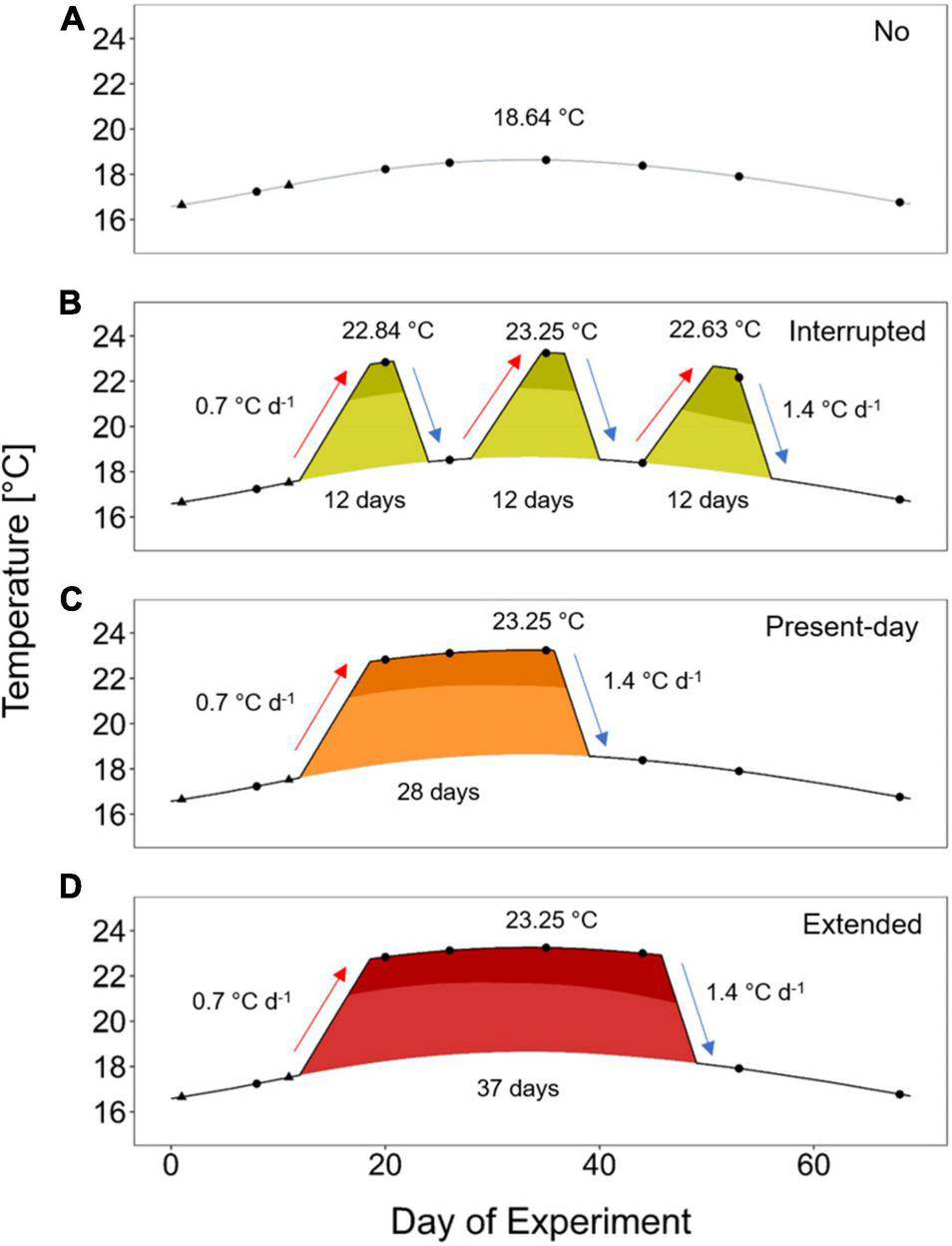
Experimental treatments based on the heatwave definition by Hobday et al. (2016). The treatments followed a smoothed natural summer seasonal temperature profile [No heatwave, gray line in panel (A); “climatological values” in Hobday et al. (2016)] or experienced three short heatwaves of 12 days each [Interrupted, yellow-green filling in panel (B)], a heatwave of 28 days [Present-day, orange filling in panel (C)] or a heatwave of an extended duration of 37 days [Extended, red filling in panel (D)]. Durations refer to the period with temperatures above the climatological values. Temperatures above the 90th percentile are shown in a darker shade. All heatwaves had a maximum peak of +4.6°C above the climatological values. Mean temperatures of the Interrupted and Present-day heatwave treatments were equal. Black triangles represent measuring points for wet weight of A. rubens, and black dots indicate additional assessments of righting responses.
Experimental Set-Up
The treatments were applied in the Kiel Indoor Benthocosms (Pansch and Hiebenthal, 2019) from July 5th to September 10th, 2019. The KIBs are a state-of-the-art mesocosm system comprised of twelve 600 L tanks, which served as water baths for each six replicated experimental units (2 L Kautex bottles). Every treatment was applied in two separate and randomly chosen tanks leading to a replication of n = 12. Temperature was logged hourly in all ten tanks (EnvLogger, ElectricBlue, Vairão, Portugal; see Supplementary Figure 1 for attained temperatures). Additionally, temperature was monitored by measuring with a handheld thermometer at least every 3 days (TTX 110 type T, Ebro, Ingolstadt, Germany). Salinity, pH and oxygen concentration were also monitored over the experimental period (Multi 3630 IDS, WTW, Kaiserslautern, Germany; see Supplementary Figure 2). Each of the 72 experimental units contained one separate sea star individual. Though six of the experimental units were placed in the same tank, all of them had a separate water inflow and aeration and were thus considered as independent replicates, yet, potential tank effects were accounted for in the model by including the individual sea star as random factor (see “Data Analysis” below). The temperature in each of the tanks is automatically controlled via chillers and heating elements (Pansch and Hiebenthal, 2019). Due to a short malfunctioning of the system, oxygen levels in the experimental units dropped to circa 2 mg L–1 (pH down to 7.1) for one out of 68 days in all treatments (Supplementary Figure 2). As this stress was only experienced for a short time, presumably all starfish were impacted equally, and we did not observe any impacts on the sea stars (such short-term hypoxic events are relatively common in the area with 18 days of upwelling favorable winds per summer; Karstensen et al., 2014), we continued with the experiment.
The Study Organism
We collected A. rubens individuals in Möltenort, Kiel, Germany (N54°22′57.5″, E010°12′8.8″) on July 1st, 2019. Directly after collection, all sea stars were brought to a climate room and placed inside a 600 L tank with a temperature of 18°C as was measured at the collection site while sampling. The sea stars were fed ad libitum with blue mussels. When starting the experiment only sea stars of similar weight (11.3 ± 1.4 g SD) were used.
Response Variables
We measured feeding rate (mg mussel dry weight per day), wet weight change (g) and righting time as a measure for the activity of A. rubens (min). For feeding rate, blue mussels (Mytilus spp.) between 1.5 and 2 cm shell length were collected the day prior to the feeding at piers next to GEOMAR, Kiel, Germany (N54°19′45.8″, E010°08′56.4″). At each feeding event, mussels inside each experimental unit were replaced with the freshly collected mussels. At the same time, we measured the shell length of consumed mussels (Dial Caliper DialMax Metric, Wiha Division KWB Switzerland). As previously described, the mussel’s shell length and tissue dry weight correlate strongly [Supplementary Material in Morón Lugo et al. (2020)]. Therefore, we used this correlation to estimate the dry weight of mussels consumed by the sea stars. Wet weight of the sea stars was measured at the start of the experiment, right before the heatwaves started, before the Present-day heatwave started to decline, before the Extended heatwave started to decline and at the end of the experiment (Figure 1). The righting time was measured by turning the sea star on its aboral side and stopping the time it needed to fully turn back on its oral side (Lawrence and Cowell, 1996). These measurements were taken at the same days as weighing (Figure 1) to reduce unnecessary handling stress for the sea stars.
Data Analysis
All data were analyzed using R (R Core Team, 2021).
The trends of extreme event properties were analyzed using Generalized Additive Models (GAMs), applying the function bam from the package “mgcv” (Wood, 2017). The models were fitted assuming Gaussian distribution of errors for all parameters, but for frequency of events. As the frequency represents count data, a Poisson distribution of errors was assumed. The smooth terms for all peak dates and months were adjusted using thin plate regression splines, while the smoothing parameters were estimated via Restricted Maximum Likelihood (Wood, 2017). For duration and cumulative intensity an additional autocorrelation factor rho was included in the model.
We analyzed the impact of our treatments over time on the performance (feeding rate, wet weight and righting time) of A. rubens using sophisticated regression approaches. We used Generalized Additive Mixed-effects Models (GAMMs) for identifying trends in feeding rate and righting time over the course of the experiment. Therefore, the function bam from the package “mgcv” (Wood, 2017) was used. We chose GAMMs for feeding rate and righting time as the observed pattern was complex and not linear. The models were fitted assuming Gaussian distribution of errors. The smooth terms for all applied treatments over the experimental period were adjusted using thin plate regression splines, while the smoothing parameters were estimated via REML (Wood, 2017). As all measurements were repeated through time on the same individuals, identity of the respective individual (i.e., replicate) was included as random effect. The temporal trends of the GAMMs in the different treatments were compared using the function plot_diff found in the package “itsadug” (van Rij et al., 2020).
TABLE 1
| GAMM feeding rate |
|||||
| Parametric coefficients | Estimate | Std. error | t-Value | p-Value | |
| Intercept | 55.46 | 2.36 | 23.49 | <0.001 | |
| Interrupted | –17.25 | 2.54 | –6.80 | <0.001 | |
| Present-day | –31.33 | 2.42 | –12.93 | <0.001 | |
| Extended | –43.65 | 2.45 | –17.80 | <0.001 | |
|
|
|||||
| Smooth terms | Estimated d.f. | Reference d.f. | F-value | p-value | |
|
|
|||||
| s (Day of experiment) | 1.015 | 1.028 | 285.750 | <0.001 | |
| s (Day of experiment): Interrupted | 1.952 | 1.997 | 15.253 | <0.001 | |
| s (Day of experiment): Present-day | 1.990 | 2.000 | 54.139 | <0.001 | |
| s (Day of experiment): Extended | 1.984 | 2.000 | 65.768 | <0.001 | |
| s (Replicate) | 0.808 | 1.000 | 4.195 | 0.023 | |
|
|
|||||
| LMM feeding rate | |||||
|
|
|||||
| Contrast | Estimate | Std. error | d.f. | t-Value | p-Value |
|
|
|||||
| No:Interrupted | 18.700 | 5.220 | 42.000 | 3.585 | 0.005 |
| No:Present-day | 30.400 | 5.110 | 42.000 | 5.952 | <0.001 |
| No:Extended | 42.500 | 5.110 | 42.000 | 8.306 | <0.001 |
| Interrupted:Present-day | 11.700 | 5.110 | 42.000 | 2.289 | 0.117 |
| Interrupted:Extended | 23.700 | 5.110 | 42.000 | 4.644 | <0.001 |
| Present-day:Extended | 12.000 | 5.000 | 42.000 | 2.408 | 0.091 |
Generalized Additive Mixed-effect Model (GAMM) and Linear Mixed-effect Model (LMM) results for feeding rate (mg mussel dry weight per day) over 68 days of incubation.
The GAMM for feeding rate had an explained deviance of 54.8%. Significant effects are shown in bold.
In contrast to feeding rate and righting time, the pattern for wet weight was linear, so we applied a Linear Mixed-effect Model (LMM) showing the growth trends over time. Therefore, the function lmer from the package “lme4” (Bates et al., 2015) was used, in which the interaction between time and treatment was included, to elucidate the changes over the experimental period subjected to our applied treatments. To account for the repeated measurements of the same individual, we included individual identity as random effect. Identically as for the GAMMs, REML was used to estimate smoothing parameters.
An LMM using REML was applied to identify the impact of the three consecutive heatwaves in the Interrupted heatwave treatment on the average feeding rate during each heatwave event. This was compared to the feeding rate in the No heatwave treatment during the same periods. Therefore, we included the interaction between treatment and the heatwave event as fixed effects, as well as identity of individuals as random effect.
For all response variables an additional LMM was applied using REML to identify the treatment’s overall impact at the end of the experiment. In these models, only the treatment as fixed effect and the identity of individuals as random effect were included. The output for all LMMs were generated via the function emmeans of the equally named package, in which the contrast analysis is based on a Tukey-test (Lenth, 2020).
The assumptions for all models were thoroughly checked via visual inspection of residual plots.
TABLE 2
| LMM wet weight |
|||||
| Parametric coefficients | Estimate | Std. Error | d.f. | t-Value | p-Value |
| Intercept | 10.195 | 0.899 | 55.088 | 11.346 | <0.001 |
| Interrupted | 0.789 | 1.271 | 55.088 | 0.621 | 0.537 |
| Present-day | 0.268 | 1.245 | 55.294 | 0.215 | 0.830 |
| Extended | 2.259 | 1.245 | 55.294 | 1.814 | 0.075 |
| Day of experiment | 0.287 | 0.011 | 362.029 | 26.355 | <0.001 |
| Interrupted:Day of experiment | –0.111 | 0.015 | 362.029 | –7.225 | <0.001 |
| Present-day:Day of experiment | –0.200 | 0.015 | 362.061 | –13.216 | <0.001 |
| Extended:Day of experiment | –0.250 | 0.015 | 362.061 | –16.579 | <0.001 |
|
|
|||||
| Contrast | Estimate | Std. error | d.f. | t-Value | p-Value |
|
|
|||||
| No:Interrupted | 2.496 | 1.190 | 41.900 | 2.102 | 0.169 |
| No:Present-day | 5.609 | 1.160 | 42.000 | 4.822 | <0.001 |
| No:Extended | 5.134 | 1.160 | 42.000 | 4.413 | <0.001 |
| Interrupted:Present-day | 3.114 | 1.160 | 42.000 | 2.677 | 0.050 |
| Interrupted:Extended | 2.638 | 1.160 | 42.000 | 2.268 | 0.122 |
| Present-day:Extended | –0.476 | 1.140 | 42.100 | –0.418 | 0.975 |
Linear Mixed-effect Model results for the wet weight (g) over 68 days of incubation.
Significant effects are shown in bold.
TABLE 3
| GAMM righting time |
|||||
| Parametric coefficients | Estimate | Std. error | t-Value | p-Value | |
| Intercept | 147.577 | 13.777 | 10.712 | < 0.001 | |
| Present-day | –21.904 | 19.483 | –1.124 | 0.262 | |
| Interrupted | 17.506 | 19.129 | 0.915 | 0.361 | |
| Extended | 83.577 | 19.129 | 4.369 | < 0.001 | |
|
|
|||||
| Smooth terms | Estimated d.f. | Reference d.f. | F-Value | p-Value | |
|
|
|||||
| s (Day of experiment) | 2.264 | 2.734 | 1.487 | 0.304 | |
| s (Day of experiment): Interrupted | 1.003 | 1.006 | 0.002 | 0.985 | |
| s (Day of experiment): Present-day | 3.555 | 3.864 | 4.672 | 0.004 | |
| s (Day of experiment): Extended | 3.776 | 3.958 | 9.894 | < 0..001 | |
| s (Individual) | 0.000 | 1.000 | 0.000 | 0.943 | |
|
|
|||||
| LMM righting time | |||||
|
|
|||||
| Contrast | Estimate | Std. error | d.f. | t-Value | p-Value |
|
|
|||||
| No:Interrupted | 0.365 | 0.473 | 41.700 | 0.771 | 0.867 |
| No:Present-day | –0.283 | 0.464 | 42.000 | –0.611 | 0.928 |
| No:Extended | –1.400 | 0.464 | 42.000 | –3.018 | 0.022 |
| Interrupted:Present-day | –0.648 | 0.464 | 42.000 | –1.398 | 0.508 |
| Interrupted:Extended | –1.765 | 0.464 | 42.000 | –3.805 | 0.003 |
| Present-day:Extended | –1.116 | 0.454 | 42.200 | –2.457 | 0.082 |
Generalized Additive Mixed-effect Model and LMM results for righting time (min) over 68 days of incubation.
The GAMM for feeding rate had an explained deviance of 24.9%. Significant effects are shown in bold.
Results
Heatwave Characteristics and Trends
Between 1997 and 2018, only the onset rate of cold-spells decreased significantly (Supplementary Figure 3E). All other parameter of cold-spells as well as heatwaves did not change significantly during this time (Supplementary Figures 3, 4). Though, cold-spells tended to increase in duration and cumulative intensity (Supplementary Figures 3B,D), while maximum intensity and decline rate tended to decrease (Supplementary Figures 3C,F). Cold-spell frequency and all heatwave characteristics on the other hand, did not show any trend (Supplementary Figures 3A, 4A–F). Although, date of occurrence of the extreme events did mostly not significantly explain the given trend, the maximum intensity, onset and decline rate for heatwaves as well as cold-spells differed significantly between months (Supplementary Figures 3C,E,F, 4C,E,F). Generally, cold years favored cold-spells, whereas warm years favored heatwaves (Supplementary Figure 5 and Figure 2).
FIGURE 2
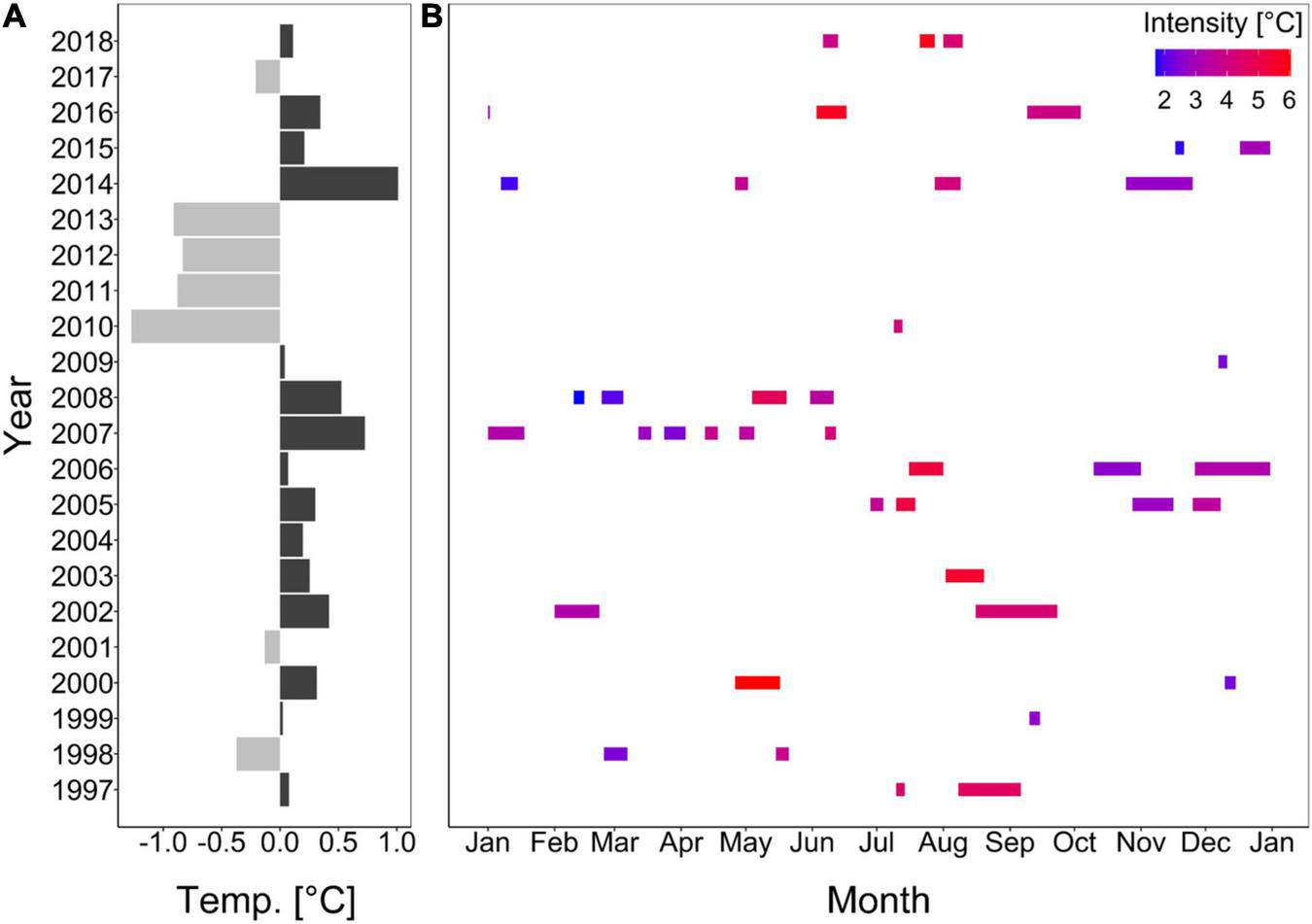
Deviations from annual mean seawater temperature from a 22-year mean (A; Wolf et al., 2020) and heatwave durations in different months over the 22-year record (B). Colors in panel (A) represent cold (light gray) or warm (dark gray) years, and in panel (B) the intensity of the heatwave (i.e., maximum amplitude above the climatological value).
Heatwaves usually occur 1.8 times per year with a mean duration of 14.9 days and an intensity of 3.6°C (Supplementary Table 1). At the same time, cold-spells occur twice per year on average with a mean duration and intensity of 12.7 days and 3.7°C, respectively (Supplementary Table 2). These parameters differ throughout the seasons (Supplementary Tables 1, 2).
Feeding Rates Over Time
Sea stars (A. rubens) increased their feeding rate over the 68-days experiment but stopped feeding immediately as soon as the heatwave started in both, the Present-day and Extended heatwave treatments (Figure 3A). Yet, sea stars in the Present-day heatwave treatment fed on as many mussels as in the No heatwave treatment by the end of the experiment (Figure 3A). Feeding rates were also reduced in the Interrupted heatwave treatment, but less than in the two continuous heatwave treatments (Figure 3A). This is also indicated by the non-significant reduction of feeding rates during the first heatwave of the Interrupted heatwave treatment (Figure 4A). However, the second and third heatwave reduced the feeding rate significantly by 72 and 45%, respectively (Figures 4B,C). The reduced performance during heatwaves is further indicated by an overall diminished feeding rate in heatwave treatments, with a more severe impact the longer the event lasted (up to 99.7% decrease in the Extended compared to the No heatwave treatment; Figures 3A,B).
FIGURE 3
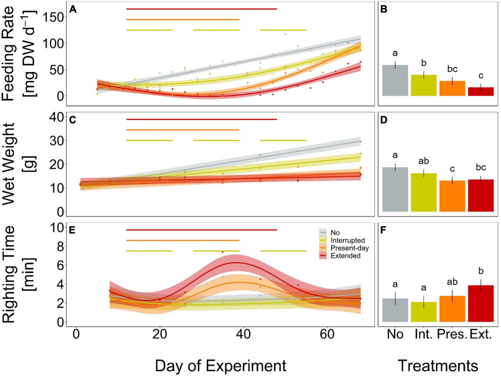
Feeding rate (mg mussel dry weight per day, A,B), wet weight (g, C,D) and righting time (minutes, E,F) of Asterias rubens during 68 days of incubation, under No (gray), Interrupted (yellow-green), Present-day (orange), and Extended (red) heatwave treatments (see Figure 1 for treatment descriptions). Measured data are represented as means for every measurement point [dots in panels (A,C,E)] and as overall means with 95% confidence intervals [bars and whiskers in panels (B,D,F)]. Temporal trends are modeled using Generalized Additive Mixed-effects Models [GAMM; solid lines in panels (A,E)] or Linear Mixed-effects Models [LMM; solid lines in panel (B)] and 95% confidence intervals [shaded areas in panels (A,C,E)]. The horizontal lines (A,C,E) represent the periods of heatwaves (Interrupted, Present-day, and Extended). Significant differences between treatments for feeding rate and righting time (A,E) are shown in Supplementary Figures 6, 7). Lower case letters in panels (B,D,F) represent significant differences between treatments based on Tukey post hoc comparisons of LMM. Results shown are based on n = 12 (Present-day and Extended) or n = 11 (No and Interrupted) replicates. Detailed statistical outcomes are given in Tables 1–3. See also Supplementary Figures 8–10 for representation of bar plots and 95% confidence intervals over time.
FIGURE 4
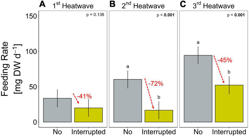
Feeding rate (mg mussel dry weight per day) during each of the three heatwaves of the Interrupted heatwave treatment and the respective period in the No heatwave treatment (A: 1st, B: 2nd and C: 3rd heatwave period). Data are presented as means (bars) and 95% confidence intervals (whiskers). Lower case letters represent significant differences between treatments based on Tukey post hoc comparisons. Percental differences between means are given in red. Detailed statistical outcomes are given in Table 4.
Wet Weights
Growth rates, as indicated by changes in weight, decreased by 39, 70, and 87% in the Interrupted, Present-day and Extended heatwave treatments when compared to the reference treatment (i.e., the No heatwave treatment), respectively (slopes of GAMMs in Figure 3C). Overall, wet weight only decreased significantly in the Present-day and Extended heatwave treatments (Figure 3D). Similarly to the feeding rates, the effect was more severe in the Extended heatwave treatment (Figures 3C,D).
Reduced Righting Time During Continuous Heatwaves
Only during the Present-day and Extended heatwave event the righting time of sea stars (a measure of activity) was significantly increased (i.e., low activity), whereas specimens in the Interrupted heatwave treatment did not show a lower activity (Figure 3E). Although sea stars were as active after the Extended heatwave had ended as before the heatwave had started, there was an overall negative impact of the Extended heatwave on the activity of the sea stars (Figure 3F).
Discussion
Heatwave Traits and Trends
Marine species are differently impacted by heat stress (e.g., Pansch et al., 2018; Gómez-Gras et al., 2019; Saha et al., 2020; Wahl et al., 2020). Therefore, defining particular temperature thresholds for marine ecosystems at the local scale and globally remains challenging. Corals have been a major research subject for global warming since the 1990s, so that much information is available to project the impact of heating events on corals (i.e., bleaching) using the concept of degree heating weeks (Liu et al., 2006). However, in order to define species-specific thresholds in diverse communities, one would need thermal performance curves for all species in the system (Schulte et al., 2011). But even if these performance curves were to exist, different traits may have different optima (Wahl et al., 2020). Thus, the whole organism response of the respective species would be a combination from all relevant traits with their potentially different optima resulting in the overall fitness. Therefore, a biology-based methodology for the characterization of heatwaves may not necessarily be the ideal approach. A physical (oceanographic) approach as applied in our study can circumvent the problem by merely focusing on time-series of temperature data and thus, modeling typical vs. extreme conditions in an environment.
Baltic Sea models project an increase in e.g., heatwave duration (Gräwe et al., 2013). Therefore, it is unlikely that the absence of trends in heatwave characteristic in the Kiel Fjord is an actual absence of a trend but rather suggests that our dataset of 22-years may not be sufficient to capture long-term trends in this naturally variable system (Reusch et al., 2018). Fluctuations in the Baltic Sea are not only apparent as extreme events or short-term temperature changes (Pansch and Hiebenthal, 2019), but even as fluctuations on an inter-annual scale as our data highlight. The years 2010–2013 were particularly cold years, which compares well to the extremely low North Atlantic Oscillation index around 2010 (Hurell and National Center for Atmospheric Research Staff, 2020). This anomalous low index (Osborn, 2011) may partly be the reason we did not detect a general warming trend in the time span tested. Yet, warming is the main driver of heatwave trends (Oliver, 2019). Therefore, longer (Hobday et al., 2016) datasets may be required in highly fluctuating systems like the Baltic Sea. This does not only mean that we might have missed existing trends, but also that we may have over- or underestimated some of the heatwave properties. A recent publication by Schlegel et al. (2019) investigated how shorter timeseries impact the differently modeled heatwave parameters. Following their findings of the median heatwave properties, our 22-year dataset should likely have 7% more heatwaves, while the duration and maximum intensity should be decreased by 6.4 and 7.3%, respectively. As we chose the heatwave properties for our experiment conservatively, the natural relevance of the study persists, especially as natural heatwaves similar to our Present-day and Extended heatwave treatment occurred in August 2003 and August 2002, respectively (Supplementary Figure 11). Therefore, our experiment provides unique insights into the performance of a keystone predator in times of extreme (and recurring) events.
Heatwaves Reduce the Performance of Asterias rubens
Daily temperatures of at least 23.25°C (maximum temperature reached in our experiment) were already measured 89 times in the Kiel Fjord over the past two decades (Wolf et al., 2020). Though not lethal, continuous heatwaves (i.e., Present-day and Extended heatwave treatments) reduced the performance of the sea star A. rubens in feeding, growth, and activity, which confirms previous findings (Rühmkorff et al., unpublished data). Similar impacts and temperature thresholds were also identified for other sea stars (Pisaster ochraceus, Pincebourde et al., 2008) and sea urchins (Heliocidaris erythrogramma, Minuti et al., 2021). Melzner et al. (personal communication) showed for echinoderms, that thermal stress causes low coelomic oxygen concentrations. Likely, the heatwaves in our experiment led to such a decreased coelomic oxygen concentration in A. rubens, so that activity and feeding rate decreased. Consequently, this reduced the growth rate of individuals. Especially, when the heatwaves were extended by 9 days, the impact on sea stars was drastic.
Sea stars in all, but the Extended heatwave treatment, fed more at the end compared to the start of the experiment (Figure 3A). On the one hand, this indicates the high recovery potential of A. rubens, but is likely also driven by the higher energy need of larger sea stars toward the end of the experiment. This elongation is similar to future extrapolation trends of heatwave duration with an increase of 10.3 days by 2100 (Oliver et al., 2018). Pincebourde et al. (2008) likewise demonstrated that longer exposure to heat stress provokes a lasting effect on sea stars. Even when the stress event may be over, echinoderms still suffer from the experienced heat stress by carry over effects (Minuti et al., 2021).
While the more robust prey of sea stars, blue mussels, were shown to survive weeks of exposure to temperatures up to 26°C in the Baltic Sea (Vajedsamiei et al., 2021) or even temperatures up to 41°C for 3 h air exposure in the eastern English Channel (Seuront et al., 2019), temperatures of already 26°C were shown to be 100% lethal for A. rubens (Rühmkorff et al., unpublished data). Similarly, Petes et al. (2008) could show that sea stars’ mortality is more pronounced in mussel beds that lay closer to the warmer water surface at an intertidal rocky shore, whereas their mussel prey proved to be more resistant to that same heat stress.
Bonaviri et al. (2017) showed that the sea star Pycnopodia helianthoides can only control its main prey, the sea urchin Strongylocentrotus purpuratus, in a non-warming scenario. Considering the fact that blue mussels are thermally more robust (Vajedsamiei et al., 2021) than sea stars and assuming that sea stars cannot adapt or temporarily migrate to deeper and colder waters, A. rubens will hardly be able to control blue mussel abundances (Reusch and Chapman, 1997) in the future Baltic Sea. Thus, a mussel dominated ecosystem might be formed (Reusch and Chapman, 1997), resulting in a restructured benthic community with overall lower diversity. At the same time, we demonstrated that summer heatwaves reduce the weight and thus the size of sea stars. As body size and prey size are strongly correlated in sea stars (Sommer et al., 1999), a heatwave summer would consequently lead to an increased predation on smaller mussels after the heatwaves have ended. This ecosystem-wide impact might be particularly strong for species-poor ecosystems such as the Baltic Sea, unless newcomers add to ecosystem diversity. In this particular case, feeding pressure on similar prey and prey size, as provoked by the recent invader Hemigrapsus takanoi (Nour et al., 2020), may add to ecosystem complexity, with yet unknown consequences. Yet, we conclude that heatwaves affect the keystone predator A. rubens with likely ecosystem-wide consequences, especially on the distribution and extent of mussel beds.
TABLE 4
| LMM feeding rate |
|||||
| Parametric coefficients | Estimate | Std. error | df | t-Value | p-Value |
| Intercept | 33.609 | 6.408 | 55.040 | 5.245 | <0.001 |
| Interrupted | –13.655 | 9.063 | 55.040 | –1.507 | 0.138 |
| Heatwave No. 2 | 26.693 | 8.044 | 40.000 | 3.318 | 0.002 |
| Heatwave No. 3 | 60.729 | 8.044 | 40.000 | 7.550 | <0.001 |
| Interrupted:Heatwave No. 2 | –29.910 | 11.375 | 40.000 | –2.629 | 0.012 |
| Interrupted:Heatwave No. 3 | –28.413 | 11.375 | 40.000 | –2.498 | 0.017 |
Linear Mixed-effect Model results for feeding rate (mg mussel dry weight per day) over the three heatwave events in the Interrupted heatwave treatment.
Significant effects are shown in bold.
Mitigated Impacts by Interrupted Heatwaves
Naturally, an interruption of a heatwave is most likely caused by a cold-spell during an upwelling event at which deeper and colder waters are shoaled to the surface (Lehmann and Myrberg, 2008; Wahl et al., 2021). Though, upwelling events in late summer are often hypoxic (Karstensen et al., 2014) and were shown to negatively impact A. rubens (Rühmkorff et al., unpublished data), they can still be beneficial when they interrupt lethal temperature extremes during heatwave events. The importance of cooling events, e.g., large-amplitude internal waves, during heat stress was already demonstrated for tropical systems (Schmidt et al., 2016). In our experiment, sea star individuals subjected to the Interrupted heatwaves fed more, were more active, and therefore grew faster than individuals exposed to continuous heatwave treatments. Yet, other fitness consequences such as reproductive success were not measured but could have long-term impacts (Melzner et al., 2020). Overall, this demonstrates that sea stars in temperate regions may quickly recover from thermal stress by using the colder periods in between heatwave events. Or in simpler words, sea stars stop feeding during the heat stress events itself, with a more pronounced impact by longer heatwaves, while resuming to feed normally after the event had ended. In contrast, findings by Morón Lugo et al. (2020), show that repeated short-term excursion into stressful conditions can be detrimental for A. rubens. Thus, mean stress levels, but also duration and amplitude of stress events and periods of recovery, will act collectively and determine the overall impact of heat stress in in a future ocean. Additionally, we provide strong evidence that environmental variability such as frequent times of stress recovery may provide a short-term refuge for sea stars from heatwave conditions projected for the future.
We show that the interruption of heatwaves did not only increase the overall performance of the temperate predator A. rubens compared to more continuous heat events, but also that the interruption has led to a significantly smaller impact of the third heatwave than the previous event, indicating some potential for acclimation. Other studies already showed that recovery time is very important for a species’ and community’s stress response (e.g., DeCarlo et al., 2019; Hughes et al., 2019; Nguyen et al., 2020) and this seems to play a crucial role also for the response of A. rubens to heatwaves. Our results might thus indicate the potential of A. rubens to gain benefits through an ecological stress memory (sensu Jackson et al., 2021). Yet, this needs further investigation, especially on the physiological mechanisms that are involved.
Conclusion
An appropriate heatwave characterization can be an extremely important tool for the design of close-to-nature experiments and can therefore help our understanding of the impact of extreme events on single species up to communities and ecosystems. The decreased performance of a temperate keystone predator in response to such simulated heatwaves has likely effects on the whole benthic ecosystem, as their main prey is an ecosystem engineer that may be released from its main predation pressure. At the same time, distinct recovery phases can play an essential role in the heatwave response of the investigated sea star A. rubens. The underlying mechanisms that trigger such acclimation and hardening processes still need to be investigated, as well as the question if long-term acclimation to continuous stressors is possible.
Publisher’s Note
All claims expressed in this article are solely those of the authors and do not necessarily represent those of their affiliated organizations, or those of the publisher, the editors and the reviewers. Any product that may be evaluated in this article, or claim that may be made by its manufacturer, is not guaranteed or endorsed by the publisher.
Statements
Data availability statement
All data obtained from the present study are stored at PANGAEA and can be accessed through the following links: https://doi.org/10.1594/PANGAEA.939981 and https://doi.org/10.1594/PANGAEA.939978.
Author contributions
FW and CP initiated and designed the study. FW and KS collected the data. FW analyzed the data and wrote the manuscript. All authors contributed to the article and approved the submitted version.
Funding
This study was funded by the Deutsche Forschungs gemeinschaft (DFG; PA2643/2/348431475), through GEOMAR (Helmholtz-Gemeinschaft) and through Deutsche Bundesstiftung Umwelt (DBU; 20018/553).
Acknowledgments
We would like to thank Mia Großmann and Sean Kearney for their help during the experiment, including mussel collection, feeding and general maintenance, and Björn Buchholz for help in maintaining the experimental facility.
Conflict of interest
The authors declare that the research was conducted in the absence of any commercial or financial relationships that could be construed as a potential conflict of interest.
Supplementary material
The Supplementary Material for this article can be found online at: https://www.frontiersin.org/articles/10.3389/fmars.2021.790241/full#supplementary-material
References
1
Banti V. Loreti E. Novi G. Santaniello A. Alpi A. Perata P. (2008). Heat acclimation and cross-tolerance against anoxia in Arabidopsis.Plant Cell Environ.311029–1037. 10.1111/j.1365-3040.2008.01816.x
2
Bates D. Mächler M. Bolker B. Walker S. (2015). Fitting linear mixed-effects models using lme4.J. Stat. Softw.671–48. 10.18637/jss.v067.i01
3
Bonaviri C. Graham M. Gianguzza P. Shears N. T. (2017). Warmer temperatures reduce the influence of an important keystone predator.J. Anim. Ecol.86490–500. 10.1111/1365-2656.12634
4
Boyd P. W. Collins S. Dupont S. Fabricius K. Gattuso J.-P. Havenhand J. et al (2018). Experimental strategies to assess the biological ramifications of multiple drivers of global ocean change-A review.Glob. Change Biol.242239–2261. 10.1111/gcb.14102
5
Budd G. C. (2008). “Asterias rubens Common starfish,” in Marine Life Information Network: Biology and Sensitivity Key Information Reviews, edsTyler-WaltersH.HiscockK. (Plymouth: Marine Biological Association of the United Kingdom).
6
DeCarlo T. M. Harrison H. B. Gajdzik L. Alaguarda D. Rodolfo-Metalpa R. D’Olivo J. et al (2019). Acclimatization of massive reef-building corals to consecutive heatwaves.Proc. Biol. Sci.286:20190235. 10.1098/rspb.2019.0235
7
Doney S. C. Ruckelshaus M. Duffy J. E. Barry J. P. Chan F. English C. A. et al (2012). Climate change impacts on marine ecosystems.Annu. Rev. Mar. Sci.411–37. 10.1146/annurev-marine-041911-111611
8
Dürr S. Wahl M. (2004). Isolated and combined impacts of blue mussels (Mytilus edulis) and barnacles (Balanus improvisus) on structure and diversity of a fouling community.J. Exp. Mar. Biol. Ecol.306181–195. 10.1016/j.jembe.2004.01.006
9
Gaymer C. F. Himmelman J. H. Johnson L. E. (2001). Distribution and feeding ecology of the seastars Leptasterias polaris and Asterias vulgaris in the northern Gulf of St Lawrence, Canada.J. Mar. Biol. Assoc.81827–843. 10.1017/S0025315401004660
10
Genin A. Levy L. Sharon G. Raitsos D. E. Diamant A. (2020). Rapid onsets of warming events trigger mass mortality of coral reef fish.Proc. Natl. Acad. Sci. U.S.A.11725378–25385. 10.1073/pnas.2009748117
11
Gómez-Gras D. Linares C. de Caralt S. Cebrian E. Frleta-Valić M. Montero-Serra I. et al (2019). Response diversity in Mediterranean coralligenous assemblages facing climate change: insights from a multispecific thermotolerance experiment.Ecol. Evol.94168–4180. 10.1002/ece3.5045
12
Gräwe U. Friedland R. Burchard H. (2013). The future of the western Baltic Sea: two possible scenarios.Ocean Dyn.63901–921. 10.1007/s10236-013-0634-0
13
Gunderson A. R. Armstrong E. J. Stillman J. H. (2016). Multiple stressors in a changing world: the need for an improved perspective on physiological responses to the dynamic marine environment.Annu. Rev. Mar. Sci.8357–378. 10.1146/annurev-marine-122414-033953
14
HELCOM (2013). Climate Change in the Baltic Sea Area: A HELMCOM Thematic Assessment in 2013. Balt. Sea Environ. Proc. 37.Helsinki: HELCOM.
15
Hobday A. J. Alexander L. V. Perkins S. E. Smale D. A. Straub S. C. Oliver E. C. J. et al (2016). A hierarchical approach to defining marine heatwaves.Prog. Oceanogr.141227–238. 10.1016/j.pocean.2015.12.014
16
Hughes T. P. Kerry J. T. Connolly S. R. Baird A. H. Eakin C. M. Heron S. F. et al (2019). Ecological memory modifies the cumulative impact of recurrent climate extremes.Nat. Clim. Change940–43. 10.1038/s41558-018-0351-2
17
Hurell J. National Center for Atmospheric Research Staff (2020). The Climate Data Guide: Hurell North Atlantic Oscillation (NAO) Index (Station Based). Available online at: https://climatedataguide.ucar.edu/climate-data/hurrell-north-atlantic-oscillation-nao-index-station-based(accessed July 23, 2021).
18
IPCC (2021). “Climate change 2021: the physical science basis,” in Contribution of Working Group I to the Sixth Assessment Report of the Intergovernmental Panel on Climate Change, edsMasson-DelmotteV.ZhaiP.PiraniA.ConnorsS. L.PéanC.BergerS.et al (Geneva: IPCC).
19
Jackson M. C. Pawar S. Woodward G. (2021). The temporal dynamics of multiple stressor effects: from individuals to ecosystems.Trends Ecol. Evol.36402–410. 10.1016/j.tree.2021.01.005
20
Karstensen J. Liblik T. Fischer J. Bumke K. Krahmann G. (2014). Summer upwelling at the Boknis Eck time-series station (1982 to 2012) – a combined glider and wind data analysis.Biogeosciences113603–3617. 10.5194/bg-11-3603-2014
21
Kayanne H. (2017). Validation of degree heating weeks as a coral bleaching index in the northwestern Pacific.Coral Reefs3663–70. 10.1007/s00338-016-1524-y
22
Lawrence J. M. Cowell B. C. (1996). The righting response as an indication of stress in Stichaster striatus (Echinodermata, asteroidea).Mar. Freshw. Behav. Physiol.27239–248. 10.1080/10236249609378969
23
Le Nohaïc M. Ross C. L. Cornwall C. E. Comeau S. Lowe R. McCulloch M. T. et al (2017). Marine heatwave causes unprecedented regional mass bleaching of thermally resistant corals in northwestern Australia.Sci. Rep.7:14999. 10.1038/s41598-017-14794-y
24
Lehmann A. Myrberg K. (2008). Upwelling in the Baltic Sea — A review.J. Mar. Syst.74S3–S12. 10.1016/j.jmarsys.2008.02.010
25
Lenth R. V. (2020). emmeans: Estimated Marginal Means, aka Least Squares means.
26
Leppäranta M. Myrberg K. (eds.) (2009). Physical Oceanography of the Baltic Sea.Berlin: Springer.
27
Liu G. Srong A. E. Skirving W. J. Arzayus L. F. (2006). “Overview of NOAA coral reef watch program’s near-real-time satellite global coral bleaching monitoring activities,” in Proceedings of the 10th International Coral Reef Symposium, Okinawa, 1783–1793.
28
McBryan T. L. Healy T. M. Haakons K. L. Schulte P. M. (2016). Warm acclimation improves hypoxia tolerance in Fundulus heteroclitus.J. Exp. Biol.219474–484. 10.1242/jeb.133413
29
Melzner F. Buchholz B. Wolf F. Panknin U. Wall M. (2020). Ocean winter warming induced starvation of predator and prey.Proc. Biol. Sci.287:20200970. 10.1098/rspb.2020.0970
30
Minuti J. J. Byrne M. Hemraj D. A. Russell B. D. (2021). Capacity of an ecologically key urchin to recover from extreme events: physiological impacts of heatwaves and the road to recovery.Sci. Total Environ.785:147281. 10.1016/j.scitotenv.2021.147281
31
Morón Lugo S. C. Baumeister M. Nour O. M. Wolf F. Stumpp M. Pansch C. (2020). Warming and temperature variability determine the performance of two invertebrate predators.Sci. Rep.10:6780. 10.1038/s41598-020-63679-0
32
Nguyen H. M. Kim M. Ralph P. J. Marín-Guirao L. Pernice M. Procaccini G. (2020). Stress memory in Seagrasses: first insight into the effects of thermal priming and the role of epigenetic modifications.Front. Plant Sci.11:494. 10.3389/fpls.2020.00494
33
Norling P. Kautsky N. (2007). Structural and functional effects of Mytilus edulis on diversity of associated species and ecosystem functioning.Mar. Ecol. Prog. Ser.351163–175. 10.3354/meps07033
34
Nour O. Stumpp M. Morón Lugo S. C. Barboza F. R. Pansch C. (2020). Population structure of the recent invader Hemigrapsus takanoi and prey size selection on Baltic Sea mussels.Aquat. Invasions15297–317. 10.3391/ai.2020.15.2.06
35
Oliver E. C. J. (2019). Mean warming not variability drives marine heatwave trends.Clim. Dyn.531653–1659. 10.1007/s00382-019-04707-2
36
Oliver E. C. J. Burrows M. T. Donat M. G. Sen Gupta A. Alexander L. V. Perkins-Kirkpatrick S. E. et al (2019). Projected marine heatwaves in the 21st century and the potential for ecological impact.Front. Mar. Sci.6:734. 10.3389/fmars.2019.00734
37
Oliver E. C. J. Donat M. G. Burrows M. T. Moore P. J. Smale D. A. Alexander L. V. et al (2018). Longer and more frequent marine heatwaves over the past century.Nat. Commun.9:1324. 10.1038/s41467-018-03732-9
38
Osborn T. J. (2011). Winter 2009/2010 temperatures and a record-breaking North Atlantic Oscillation index.Weather6619–21. 10.1002/wea.660
39
Pansch C. Hiebenthal C. (2019). A new mesocosm system to study the effects of environmental variability on marine species and communities.Limnol. Oceanogr. Methods28:16. 10.1002/lom3.10306
40
Pansch C. Scotti M. Barboza F. R. Al-Janabi B. Brakel J. Briski E. et al (2018). Heat waves and their significance for a temperate benthic community: a near-natural experimental approach.Glob. Change Biol.244357–4367. 10.1111/gcb.14282
41
Petes L. E. Mouchka M. E. Milston-Clements R. H. Momoda T. S. Menge B. A. (2008). Effects of environmental stress on intertidal mussels and their sea star predators.Oecologia156671–680. 10.1007/s00442-008-1018-x
42
Pincebourde S. Sanford E. Helmuth B. (2008). Body temperature during low tide alters the feeding performance of a top intertidal predator.Limnol. Oceanogr.531562–1573. 10.4319/lo.2008.53.4.1562
43
Pincebourde S. Sanford E. Casas J. Helmuth B. (2012). Temporal coincidence of environmental stress events modulates predation rates.Ecol. Lett.15680–688. 10.1111/j.1461-0248.2012.01785.x
44
R Core Team (2021). R: A Language and Environment for Statistical Computing.Vienna: R Foundation for Statistical Computing.
45
Reusch T. B. H. Chapman A. R. O. (1997). Persistence and space occupancy by subtidal blue mussel patches.Ecol. Monogr.67:65. 10.2307/2963505
46
Reusch T. B. H. Dierking J. Andersson H. C. Bonsdorff E. Carstensen J. Casini M. et al (2018). The Baltic Sea as a time machine for the future coastal ocean.Sci. Adv.4:eaar8195. 10.1126/sciadv.aar8195
47
Sadchatheeswaran S. Branch G. M. Robinson T. B. (2015). Changes in habitat complexity resulting from sequential invasions of a rocky shore: implications for community structure.Biol. Invasions171799–1816. 10.1007/s10530-014-0837-4
48
Saha M. Barboza F. R. Somerfield P. J. Al-Janabi B. Beck M. Brakel J. et al (2020). Response of foundation macrophytes to near-natural simulated marine heatwaves.Glob. Change Biol.26417–430. 10.1111/gcb.14801
49
Sanford E. (1999). Regulation of keystone predation by small changes in ocean temperature.Science (New York N.Y.)2832095–2097. 10.1126/science.283.5410.2095
50
Schlegel R. W. Smit A. J. (2018). heatwaveR: a central algorithm for the detection of heatwaves and cold-spells.J. Open Source Softw.3:821. 10.21105/joss.00821
51
Schlegel R. W. Oliver E. C. J. Hobday A. J. Smit A. J. (2019). Detecting marine heatwaves with sub-optimal data.Front. Mar. Sci.6:737. 10.3389/fmars.2019.00737
52
Schmidt G. M. Wall M. Taylor M. Jantzen C. Richter C. (2016). Large-amplitude internal waves sustain coral health during thermal stress.Coral Reefs35869–881. 10.1007/s00338-016-1450-z
53
Schulte P. M. Healy T. M. Fangue N. A. (2011). Thermal performance curves, phenotypic plasticity, and the time scales of temperature exposure.Integr. Comp. Biol.51691–702. 10.1093/icb/icr097
54
Seuront L. Nicastro K. R. Zardi G. I. Goberville E. (2019). Decreased thermal tolerance under recurrent heat stress conditions explains summer mass mortality of the blue mussel Mytilus edulis.Sci. Rep.9:17498. 10.1038/s41598-019-53580-w
55
Smale D. A. Wernberg T. Oliver E. C. J. Thomsen M. Harvey B. P. Straub S. C. et al (2019). Marine heatwaves threaten global biodiversity and the provision of ecosystem services.Nat. Clim. Change9:360. 10.1038/s41558-019-0412-1
56
Sommer U. Meusel B. Stielau C. (1999). An experimental analysis of the importance of body-size in the seastar-mussel predator-prey relationship.Acta Oecol.2081–86. 10.1016/S1146-609X(99)80019-8
57
Thomsen M. S. Mondardini L. Alestra T. Gerrity S. Tait L. South P. M. et al (2019). Local extinction of bull kelp (Durvillaea spp.) due to a marine heatwave.Front. Mar. Sci.6:84. 10.3389/fmars.2019.00084
58
Todgham A. E. Schulte P. M. Iwama G. K. (2005). Cross-tolerance in the tidepool sculpin: the role of heat shock proteins.Physiol. Biochem. Zool. PBZ78133–144. 10.1086/425205
59
Vajedsamiei J. Wahl M. Schmidt A. L. Yazdanpanahan M. Pansch C. (2021). The higher the needs, the lower the tolerance: extreme events may select Ectotherm recruits with lower metabolic demand and heat sensitivity.Front. Mar. Sci.8:660427. 10.3389/fmars.2021.660427
60
van Rij J. Wieling M. Baayen R. H. van Rijn H. (2020). itsadug: Interpreting Time Series and Autocorrelated Data Using GAMMs.
61
Vevers H. G. (1949). The biology of Asterias rubens L: growth and reproduction.J. Mar. Biol. Assoc.28165–187. 10.1017/S0025315400055272
62
Wahl M. Barboza F. R. Buchholz B. Dobretsov S. Guy-Haim T. Rilov G. et al (2021). Pulsed pressure: fluctuating impacts of multifactorial environmental change on a temperate macroalgal community.Limnol. Oceanogr.33:477. 10.1002/lno.11954
63
Wahl M. Buchholz B. Winde V. Golomb D. Guy-Haim T. Müller J. et al (2015). A mesocosm concept for the simulation of near-natural shallow underwater climates: the Kiel Outdoor Benthocosms (KOB).Limnol. Oceanogr. Methods13651–663. 10.1002/lom3.10055
64
Wahl M. Werner F. J. Buchholz B. Raddatz S. Graiff A. Matthiessen B. et al (2020). Season affects strength and direction of the interactive impacts of ocean warming and biotic stress in a coastal seaweed ecosystem.Limnol. Oceanogr.65807–827. 10.1002/lno.11350
65
Walter J. Jentsch A. Beierkuhnlein C. Kreyling J. (2013). Ecological stress memory and cross stress tolerance in plants in the face of climate extremes.Environ. Exp. Bot.943–8. 10.1016/j.envexpbot.2012.02.009
66
Walther G.-R. Post E. Convey P. Menzel A. Parmesan C. Beebee T. J. C. et al (2002). Ecological responses to recent climate change.Nature416389–395. 10.1038/416389a
67
Wolf F. Bumke K. Wahl S. Nevoigt F. Hecht U. Hiebenthal C. et al (2020). High resolution water temperature data between January 1997 and December 2018 at the GEOMAR pier surface. PANGAEA. 10.1594/PANGAEA.919186
68
Wood S. N. (2017). Generalized Additive Models.Boca Raton, FL: CRC Press.
Summary
Keywords
climate change, warming (heating), environmental fluctuation, extreme events, marine heatwaves (MHWs), mitigation, recovery
Citation
Wolf F, Seebass K and Pansch C (2022) The Role of Recovery Phases in Mitigating the Negative Impacts of Marine Heatwaves on the Sea Star Asterias rubens. Front. Mar. Sci. 8:790241. doi: 10.3389/fmars.2021.790241
Received
06 October 2021
Accepted
28 December 2021
Published
24 February 2022
Volume
8 - 2021
Edited by
Gretchen E. Hofmann, University of California, Santa Barbara, United States
Reviewed by
Simon Morley, British Antarctic Survey (BAS), United Kingdom; Sam Dupont, University of Gothenburg, Sweden
Updates
Copyright
© 2022 Wolf, Seebass and Pansch.
This is an open-access article distributed under the terms of the Creative Commons Attribution License (CC BY). The use, distribution or reproduction in other forums is permitted, provided the original author(s) and the copyright owner(s) are credited and that the original publication in this journal is cited, in accordance with accepted academic practice. No use, distribution or reproduction is permitted which does not comply with these terms.
*Correspondence: Fabian Wolf, fabian.wolf.research@gmail.com
†ORCID: Fabian Wolf, orcid.org/0000-0002-0955-8487; Katja Seebass, orcid.org/0000-0001-6520-7369; Christian Pansch, orcid.org/0000-0001-8442-4502
This article was submitted to Global Change and the Future Ocean, a section of the journal Frontiers in Marine Science
Disclaimer
All claims expressed in this article are solely those of the authors and do not necessarily represent those of their affiliated organizations, or those of the publisher, the editors and the reviewers. Any product that may be evaluated in this article or claim that may be made by its manufacturer is not guaranteed or endorsed by the publisher.