Abstract
Monitoring the spatial distribution and seasonal dynamics of phytoplankton functional types (PFTs) in coastal oceans is essential for understanding fisheries production, changes in water quality, and carbon export to the deep ocean. The launch of new generation ocean color sensors such as OLCI (Ocean Land Color Instrument) onboard Sentinel 3A provides an unprecedented opportunity to study the surface dynamics of PFTs at high spatial (300 m) and temporal (daily) resolution. Here we characterize the seasonal dynamics of the major PFTs over the surface waters of the west coast of Canada using OLCI imagery and Chemical Taxonomy (CHEMTAX, v1.95) software. The satellite-based approach was adapted from a previously proven Empirical Orthogonal Function (EOF)-based algorithm by using a local matchup dataset comprising CHEMTAX model output and EOF scores derived from OLCI remote sensing reflectance. The algorithm was developed for the following PFTs: diatoms, dinoflagellates, dictyochophytes, haptophytes, green algae, cryptophytes, cyanobacteria, raphidophytes, and total chlorophyll-a (TChla) concentration. Of these PFTs, first level evaluation of the OLCI-derived retrievals showed reliable performance for diatoms and raphidophytes. The second level of validation showed that TChla had the best performance, and green algae, cryptophytes, and diatoms followed seasonal trends of a high temporal resolution in situ CHEMTAX time-series. Somewhat reduced correspondence was observed for raphidophytes. Due to their low contribution to the phytoplankton community (26%) and low range of variation, weak performance was noted for haptophytes, dictyochophytes, cyanobacteria, and dinoflagellates. The EOF-based PFT maps from daily OLCI imagery showed seasonal spring and fall diatom blooms with succession from spring blooms to high diversity flagellate dominated summer conditions. Furthermore, strong localized summer raphidophyte blooms (Heterosigma akashiwo) were observed, which are a regionally important harmful species. Overall, this study demonstrates the potential of the OLCI in deriving the surface dynamics of major PFTs of the Strait of Georgia (SoG), a critical habitat for the juvenile Pacific Salmon.
1 Introduction
Phytoplankton represent only 0.2% of global primary producer biomass; however, they are responsible for more than 90% of the ocean’s primary productivity (Chassot et al., 2010), including half of the biosphere’s net primary productivity (Field et al., 1998). These ubiquitous single-celled autotrophs are the base of the marine food web (Falkowski, 2012), and are capable of fixing ~50-130 million tons of atmospheric carbon dioxide (CO2) daily into the form of organic materials, playing a central role in the global biogeochemical cycles (Behrenfeld et al., 2006). Numerous in situ methods are available to quantify size fractions and community composition of phytoplankton in the ocean, yet these observations are time-consuming, labor-intensive, and sparse in space and time (IOCCG, 2014; Chase et al., 2017).
Space-based optical sensors measure water-leaving radiance in multiple wavebands, allowing the retrieval of the surface total chlorophyll-a (hereafter TChla), a proxy for phytoplankton biomass, with high spatial and temporal resolutions (McClain, 2009). Nevertheless, TChla alone is not sufficient to describe the ecological and biogeochemical processes in the ocean (Bracher et al., 2017). Extracting information about phytoplankton functional types (PFTs), and phytoplankton size classes (PSCs), is essential for understanding the linkage between phytoplankton composition and fisheries, and in determining the role of the ocean in a changing climate (e.g., Falkowski et al., 1998; Le Quere et al., 2005; IOCCG, 2014). Considering the highly diverse nature (e.g., taxonomical, morphological, and physiological) of marine phytoplankton, climatologists and marine biogeochemical modelers have defined PFTs according to their specific function or role in the biogeochemical cycles irrespective of their taxonomical affiliations (Le Quere et al., 2005; Nair et al., 2008). For example, diatoms are considered to be essential silicifiers, cyanobacteria as nitrogen fixers, Haptophytes as calcifiers, and Dinoflagellates/Haptophytes/Green Algae as dimethyl sulphide producers (DMSP) (IOCCG, 2014).
Given the importance of determining phytoplankton from space, several satellite-based algorithms have been developed to identify the significant PFTs (e.g., Alvain et al., 2005; Navarro et al., 2014; Correa-Ramirez et al., 2018), derive the chlorophyll-a concentration (hereafter Chla) of PFTs (e.g., Bracher et al., 2009; Sadeghi et al., 2012; Moisan et al., 2017), retrieve PSCs (e.g., Ciotti et al., 2002; Kostadinov et al., 2009; Mouw and Yoder, 2010; Brewin et al., 2010; Devred et al., 2011; Hirata et al., 2011; Brotas et al., 2013; Roy et al., 2013; Lamont et al., 2018; Moore and Brown, 2020; Liu et al., 2021), and retrieve accessory pigment concentrations (e.g., Pan et al., 2010; Bracher et al., 2015; Wang et al., 2018; El Hourany et al., 2019; Stock and Subramaniam, 2020; Kramer et al., 2022). These satellite-based algorithms explore specific signatures, such as anomalies in the reflectance spectra, inherent optical properties (IOPs), including TChla concentration (see IOCCG, 2014; Mouw et al., 2017; Bracher et al., 2017 for a detailed review). Of the many approaches developed, the Empirical Orthogonal Function (EOF) approach has been successfully used among these algorithms (e.g., Craig et al., 2012). The EOF approach is a statistical technique that reduces the high dimensionality of spectral data into dominant modes, explaining the variance of structures in the data. Specifically, the EOF approach allows the extraction of the spectral signature associated with specific PFTs, thus enabling the development of empirical models for various PFTs (e.g., Xi et al., 2020). This approach has been successful in retrieving the concentration of different accessory pigments from Medium Resolution Imaging Spectrometer (MERIS) and hyperspectral data (Bracher et al., 2015), Chla concentration of multiple PFTs using GlobColor merged and OLCI data (Xi et al., 2020), and cell abundance of Prochlorococcus, Synechococcus, and autotrophic picoeukaryotes based on multispectral and hyperspectral data (Lange et al., 2020). However, most of these studies were performed in open oceans or optically Case-1 type waters, with less application to coastal systems (e.g., Craig et al., 2012).
The coastal ocean of British Columbia, Canada, specifically the Strait of Georgia, is a spatially and temporally dynamic Case-2 water body (Phillips and Costa, 2017) crucial for Pacific salmon, herring, and hake fisheries (Beamish et al., 1994; Beamish et al., 2012; Thomson et al., 2012), which are of vital importance to the regional economy and First Nations (Nesbitt and Moore, 2016). In these waters, phytoplankton have been shown to be associated with the growth and survival of these species (Cushing, 1990) through their bottom-up control of key zooplankton species such as Neocalanus plumchrus (e.g., Sastri and Dower, 2009; Perry et al., 2021; Suchy et al., 2022). Hence, spatial-temporal satellite-derived PFTs will allow for a more coherent understanding of the function/role of multiple PFTs on the regional food web.
Here, we adapted an EOF-based algorithm developed by Xi et al. (2020) to the Strait of Georgia, British Columbia (BC), Canada, to retrieve TChla concentration and the Chla concentration of multiple PFTs. The model was developed for each PFT using the matchup between CHEMTAX-derived PFTs and EOF scores derived from the OLCI remote sensing reflectance (Rrs; sr–1(λ)). The robustness of the fitted regression model was assessed statistically by the cross-validation procedure, and independent validation of the major derived PFTs was performed against an independent in situ CHEMTAX time-series. Further, the seasonal and spatial dynamics of major PFTs were determined by applying the regression model to daily OLCI imagery.
2 Materials and methods
2.1 Study area
The Strait of Georgia (SoG) is the largest semi-enclosed estuarine system in the Salish Sea, located on the west coast of Canada (Figure 1). This partially enclosed region has a total length of 222 km, a maximum width of 28 km, and a depth of about 350 m within its central region (Masson and Peña, 2009), which is generally divided into three marine areas: the southern, central, and northern Strait. The SoG is connected to the Pacific Ocean through the Johnstone Strait in the northern region and Juan de Fuca Strait in the southern boundary (Peña et al., 2016). An estuarine circulation typically drives the SoG regional dynamics, characterized by low saline surface waters from the adjacent Fraser River and highly saline nutrient-rich subsurface waters from the Pacific Ocean (Li et al., 2000; Masson and Cummins, 2004). The largest freshwater discharge to the SoG is from the Fraser River, which contributes 75% of the freshwater to the Strait, and is primarily responsible for the water column stratification and estuarine-like circulation in the central and southern Strait (Harrison et al., 1983; Johannessen et al., 2003; Pawlowicz et al., 2007). Incoming seawater dominantly enters the SoG through the southern Juan de Fuca Strait (Masson, 2002), bringing nutrient-rich water from the Pacific Ocean through the deep water inflow and is eventually upwelled into the surface waters by rigorous tidal mixing in the Haro Strait (Li et al., 2000). In the summer, the northern Strait becomes highly stratified, limiting surface nutrient renewal. This stratification is thought to be a function of high summer surface heating, low summer winds, and localized freshwater discharge, and can periodically be disrupted by strong wind events (Evans et al., 2019).
Figure 1
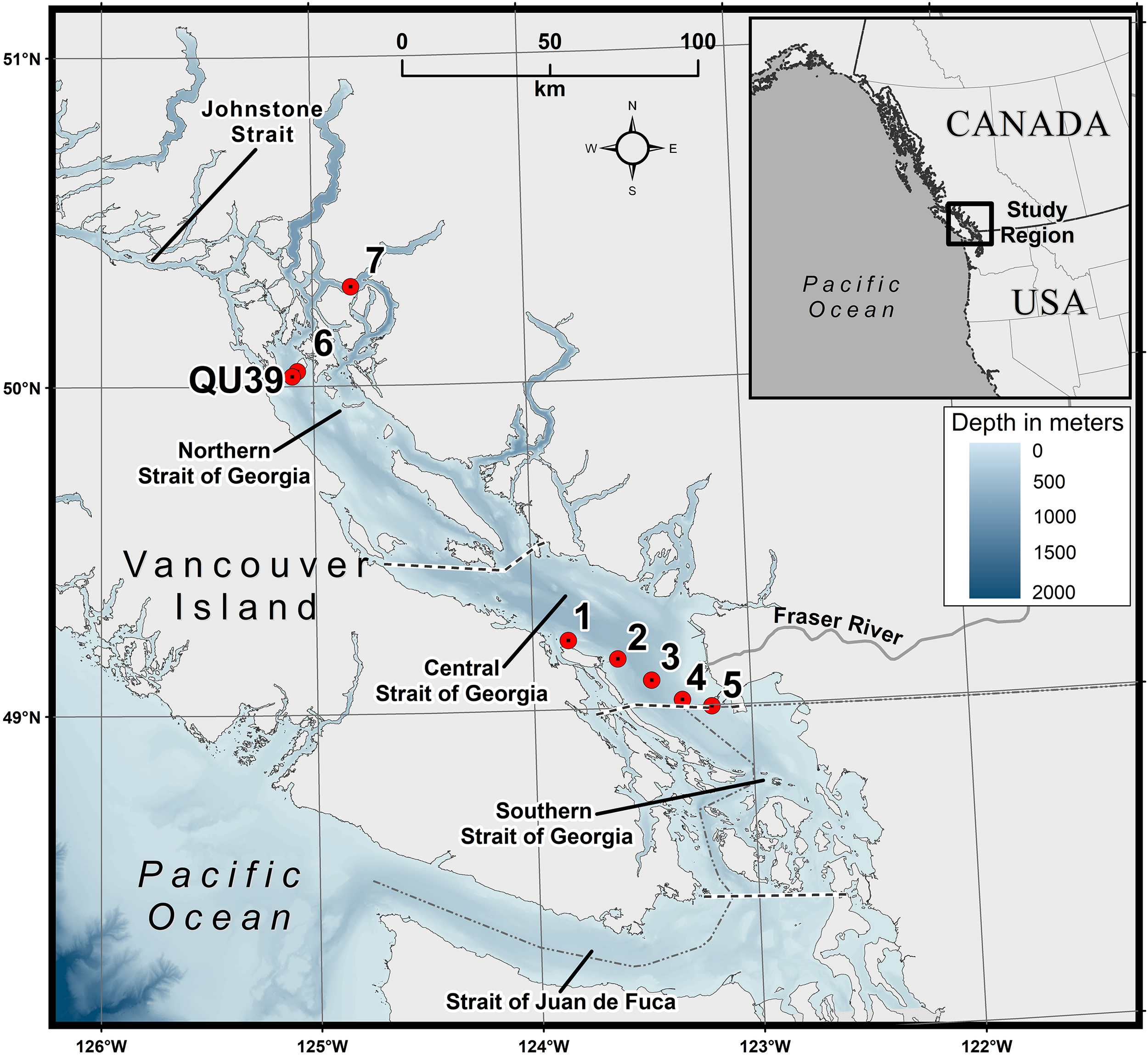
Map showing the study area. The red circles indicate the sampling locations in the central and northern Strait of Georgia (SoG). QU39 represents the Hakai time-series station. Bathymetry is shown in meters.
This region is one of the most productive estuaries in the Pacific North East with an average annual primary productivity of about 280 g C m-2, which is the highest in the frontal regions and close to the Fraser River (Harrison et al., 1983; Sutton et al., 2013; Johannessen et al., 2021). Seasonally, SoG surface TChla greatly varies with winter concentrations <1 mg m-3 and increases to > 15 mg m-3 during spring (Harrison et al., 1983; Jackson et al., 2015; Peña et al., 2016; Suchy et al., 2019). As in many temperate coastal environments, spring blooms are dominated by diatoms with Skeletonema sp., Thalassiosira spp., and Chaetoceros spp. being the dominant bloom-forming species. By the end of spring, diatoms are usually replaced by high diversity communities constituted by flagellates such as cryptophytes, dinoflagellates, prasinophytes, and haptophytes (Harrison et al., 1983; Haigh and Taylor, 1991; Del Bel Belluz et al., 2021).
Optically, the SoG is a dynamic Case-2 water body characterized by high and spectrally dependent light attenuation with estuarine waters comprised of high loads of suspended inorganic sediment and dissolved organic matter from the Fraser River discharge (Komick et al., 2009; Loos and Costa, 2010; Phillips and Costa, 2017). For these highly attenuating waters, particulate scattering varies from approximately 0.2 to 16.0 m-1 in the blue spectral region (Loos and Costa, 2010), and colored dissolved organic matter (CDOM) absorption varies from 0.007 to 3.07 m-1 (Phillips and Costa, 2017). On the other hand, total attenuation in the northern SoG is predominantly controlled by absorption by CDOM and TChla (Loos and Costa, 2010; Loos et al., 2017; Phillips and Costa, 2017).
2.2 Data acquisition
2.2.1 In situ sata: water sampling and analysis
Surface water samples were collected at two regions of the SoG. For the first location, samples (N=108) were acquired along the BC ferry route aboard the Queen of Alberni (QA) crossing from Duke Point (Nanaimo) to Tsawassen (Vancouver; Stations 1-5, Figure 1) during the spring (March to May) and summer (June to September) of 2018 and 2019. Water samples were collected using a seawater intake pump installed on the ferry, representing a well-mixed layer of <3 m (Halverson and Pawlowicz, 2013; Wang et al., 2019; Travers-Smith et al., 2021). Triplicate samples from each station were collected for the different analyses (HPLC pigment concentration, CDOM absorption, and total suspended matter (TSM) concentration), kept in a dark environment, and immediately filtered onboard to minimize any potential compositional and concentration changes to phytoplankton pigments and dissolved organic matter (Mueller et al., 2003). For the second location, the northern SoG (Stations 6-7, Figure 1), surface water samples (~ 2 m depth) (N=19) were collected during summer (July) as part of an algal bloom monitoring component at aquaculture sites. Triplicate water samples were collected using a 5 L Niskin water sampler, transferred to a 10 L dark container, transported to the laboratory in the dark, and immediately filtered for HPLC pigments, CDOM absorption, and TSM. In addition, at the northern SoG location, single samples were collected for microscopic identification and enumeration of phytoplankton species (N = 8). Water for these samples was immediately transferred to 250 mL amber glass bottles and fixed using Lugol’s solution (1% concentration); samples were kept cool and dark until analysis.
Surface water samples for the TSM were filtered through precombusted and pre-weighed 47 mm Whatman GF/F 0.7 µm filter paper. Precombustion of the filter paper increases the efficiency by retaining more particulate matter as it shrinks the pore size to 0.3 μm during combustion (Nayar and Chou, 2003). Based on the color of the seawater, filtered volumes varied from 0.5 – 2 L. After the sample filtration, the filter paper was washed with 200 ml of distilled water to remove sea salt (Stavn et al., 2009), and immediately stored in dry ice, transported to the laboratory, and kept under -80°C until analysis. The filter paper was dried at 60°C for 24 hours in a clean oven and subsequently reweighed to 6 degrees of precision, at which point TSM was calculated (Röttgers et al., 2014). The final TSM concentration at each station was the average of the triplicates with a coefficient of variation (CV) < 25%.
Surface water samples to analyze aCDOM (λ) were filtered through 47 mm Whatman 0.2 µm membrane filter paper. The filtrate was stored in acid-washed, precombusted (550°C for 1 hour) borosilicate glass bottles (Ferrari et al., 1996). Glass bottles were triple rinsed with sample water before the collection, and samples were kept in a cold environment, transferred to the laboratory and kept under 4°C until analysis. Prior to analysis, samples were allowed to reach room temperature to minimize temperature differences between the samples and the blank. The absorption of CDOM was measured using an Ocean Optics USB 4000 spectrophotometer (300-850 nm, 0.2 μm) against Milli-Q water as blank. The sample absorption was converted to CDOM absorption using Beer-Lambert’s Law equation (Ferrari et al., 1996).
A(λ) is the spectral absorption of the sample, and L is the cuvette path length in meters. The final aCDOM (λ) for each station is the average of the triplicate with a CV < 25%.
Phytoplankton microscopy was performed by LCJL Marine Ecological Services using the Utermöhl method. Phytoplankton were identified and enumerated using 50 mL settling chambers and phase contrast microscopy with an inverted light microscope (Utermöhl, 1958). Count data were reported in cells L-1. Counts from species within PFT groups used for analysis were summed to make comparisons with pigment-based estimates.
Surface water samples to measure HPLC pigments were filtered through 25 mm Whatman GF/F 0.7 µm glass microfiber filters under a low vacuum (200mm Hg/vac). Based on the color of the seawater, filtered volumes varied from 0.5 – 2 L. Filters were immediately put in dry ice and kept under -80°C until laboratory analysis. TChla and phytoplankton accessory pigments were analyzed using HPLC analysis done at the University of South Carolina Baruch Institute (https://phytoninja.com/lab-protocols/), following the methods described in Pinckney (2010). HPLC samples were collected in duplicates, and the uncertainty in the HPLC pigment dataset was computed from the duplicate measurements for 20% of the samples, resulting in a CV < 20%.
The HPLC pigment dataset was used as the input in the CHEMTAX software (v1.95) to derive the Chla concentration of each PFT towards the TChla concentration of the sample (Mackey et al., 1996). The selection of PFT and input pigment ratio were largely based on those in Del Bel Belluz et al. (2021), which were defined via in-depth analysis of pigments and pigment ratios, microscopic observations, and literature review of phytoplankton species in the SoG.
Unlike Del Bel Belluz et al. (2021), a raphidophyte group was included in the analysis to account for the extensive 2018 Heterosigma akashiwo blooms observed via microscopy at comparable sampling locations and times as those investigated in this study (Esenkulova et al., 2021). Additionally, our 2018 observations showed high violaxanthin concentration events where relationships with TChla (generally driven by diatom blooms), fucoxanthin (diatoms), Chlb (green algae), and zeaxanthin (typically only present in low concentrations and related to green algae or cyanobacteria) diverged from those through the rest of the dataset (Supplementary Material 1). During these high concentration events, fucoxanthin, violaxanthin and zeaxanthin ratios to TChla were comparable to those found for raphidophytes in the literature (Supplementary Material 2, Lewitus et al., 2005; Higgins et al., 2011). It is unlikely that other violaxanthin containing species would bloom to such high violaxanthin and TChla concentrations in the SoG. For reference, through the four-year time-series presented in Del Bel Belluz et al. (2021), which spanned multiple high TChla bloom events, violaxanthin reached a maximum concentration of 0.41 mg m-3, an order of magnitude lower than observed during this study. For the central SoG data, pigment ratios for the raphidophyte group were taken from Lewitus et al. (2005), derived from Heterosigma akashiwo. In the northern SoG, pigment and microscopic observations showed that raphidophytes were absent. As a result, this group was not included in the northern SoG analysis. With these considerations, the following groups were considered in CHEMTAX analysis: cyanobacteria-1 (Cyano), haptophytes (Hapto), green algae (GA), cryptophytes (Crypto), dinoflagellates (Dino), raphidophytes (Raphido, central SoG only), dictyochophytes (Dictyo), and diatoms (Diat). Input ratios for each taxonomic group are given in Supplementary Material 3 and Supplementary Material 4. While quantitive evaluation of CHEMTAX is often lacking, many studies have utilized similar groupings to describe phytoplankton community compositions in coastal waters (e.g., Lu et al., 2018; Ferreira et al., 2020). Here, it was decided to attempt to maximize the retrievable groups; however, it is important to note that following the methods of Catlett and Siegel (2018), clustering of the HPLC-derived pigment dataset suggests that only four PFT groups may be separatable and optically discernable (Supplementary Material 9). As a result, CHEMTAX model outputs are supported by additional information, including microscopy (northern SoG) and data from complimentary studies done at similar locations and times.
CHEMTAX analysis was run on the northern and central SoG data separately to account for regional differences in pigment ratios as a result of differing oceanographic conditions (i.e., stratification, nutrients, and light; Suchy et al., 2019). An initial seeding run was first performed on the full dataset from each region to optimize the literature-derived ratios to the SoG (Armbrecht et al., 2015; Del Bel Belluz et al., 2021). Then, the central SoG data were binned into different groups based on TSM concentrations to account for the high variability in light conditions along the ferry track and between surveys. The following TSM bins were used: Low (TSM< 5 mg/L), Medium (TSM 5 – 11 mg/L), and High (TSM > 11 mg/L), based on bio-optical classes derived by Phillips and Costa (2017) for the central SoG. CHEMTAX analysis on the binned data utilized the output ratios from the initial seeding run performed on the full central SoG dataset. For the northern SoG, TSM conditions were comparable across the surveys, and HPLC data were not binned for analysis, but a second run, using the initial seeding ratios from the full northern SoG dataset, was performed to ensure stabilized ratios and to reduce RMSE.
Beyond consideration of environmental conditions, we evaluated pigment colinearity, which can affect CHEMTAX results (Higgins et al., 2011; Catlett and Siegel, 2018). In this study, positive correlations did exist between pigments used for analysis (Supplementary Material 5). When standardized to TChla, many of these correlations were still strong (e.g., Chlb and prasinoxanthin, Supplementary Material 5); however, none were correlated with TChla. Careful consideration was taken in the CHEMTAX design to limit error; however, pigment colinearity can add bias to the CHEMTAX model output and complicate retrieval via satellite (Higgins et al., 2011; Catlett and Siegel, 2018). As independent validation of CHEMTAX model outputs was not performed here, it was difficult to quantify this error, and this is further discussed in section 4.1. Care should be taken to extend results until extensive validation has been performed.
Following the CHEMTAX analysis, we also performed a Shannon-Weaver Index (Lohrenz et al., 2003; Latasa et al., 2010) on the CHEMTAX model output to assess the diversity of phytoplankton community composition:
where, Pi is the proportion of each phytoplankton group’s Chla relative to the TChla concentration (%), and N is the number of groups.
2.2.2 Satellite data
High spatial (300 m) and temporal resolution (daily) OLCI data were used in this study as this sensor has improved signal-to-noise ratios and an off-nadir tilted view to minimize the effect of sun glint (Donlon et al., 2012). Therefore, OLCI Level-1 Full-Resolution data were downloaded from the Sentinel 3 Marine CODA (Copernicus Online Data Access) web service, and processed with POLYMER (POLYnomial-based algorithm applied to MERIS) version 4.10 (Steinmetz et al., 2011) to obtain Rrs. POLYMER is an atmospheric correction (AC) algorithm that separates the atmospheric and sunglint spectral reflectance from the water reflectance using a spectral matching technique (Steinmetz et al., 2011). To do so, it uses two models: a simple polynomial used to model the spectral reflectance from atmospheric and residual sunglint, and a model that delineates ocean water reflectance using TChla concentration and the particle backscattering coefficient (Park and Ruddick, 2005). The water reflectance model used in this algorithm is valid in coastal and open ocean waters, including the bidirectional reflectance, and it provides better spatial coverage retrievals because it accounts for sky glint and thin cloud conditions (Steinmetz et al., 2011). Quality flags such as “Cloud,” “Invalid,” “Negative Backscattering (BB),” “Out-of-bounds,” “Exception,” and “High Air Mass” (Steinmetz et al., 2016) were applied following Giannini et al. (2021) recommendations for this region. According to the technical document (Steinmetz et al., 2016), the “Inconsistency” flag should not invalidate the results; however, our matchup analysis showed artifacts with pixels associated with this flag. As a result, data with this flag were removed from analysis. Giannini et al. (2021) demonstrated that POLYMER OLCI-derived products such as TSM and TChla showed the best performance compared to the Case-2 Regional CoastColor (C2RCC) processor for the coastal waters of BC and Northeast Alaska.
2.3 Data analysis: PFT satellite-based method and validation
The Chla concentration of PFTs was derived from OLCI satellite imagery using the EOF-based algorithm by assessing the variance or spectral shape in the OLCI Rrs spectra (Bracher et al., 2015). This algorithm was recently tested globally by Xi et al. (2020), and we further adapted it considering the local matchups between OLCI Rrs and the CHEMTAX-derived PFTs Chla. A schematic workflow of the EOF-PFT algorithm is shown in Figure 2. The general steps of this approach are explained as follows:
Figure 2
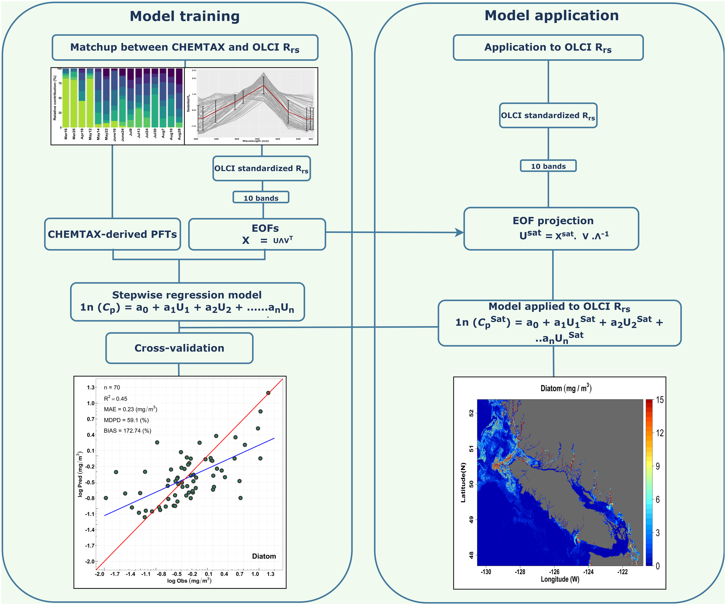
Schematic flowchart illustrating the EOF-based algorithm for predicting multiple Phytoplankton Functional Types (PFTs). The left side demonstrates the model training part with matchup comprised of CHEMTAX model output and Ocean Land Color Instrument (OLCI) remote sensing reflectance (Rrs; sr–1(λ)). The right side indicates the model application to OLCI imagery to derive the spatial distribution of PFTs.
Step 1: OLCI Rrs data at 10 bands (400, 412, 443, 490, 510, 560, 620, 665, 674, 681 nm) were standardized by subtracting the spectral average and normalized by the spectral standard deviation according to Xi et al. (2020). The standardized Rrs was then subjected to a singular value decomposition (SVD) to derive the EOF scores (U), singular values (Λ), and EOF loadings (V).
The dataset used in step 1 corresponds to matchup satellite data obtained from a 3×3 pixel window (900 × 900 m) centered around the in situ sampling region and meeting the following criteria: ± 3 hours time difference, valid pixels are ≥5/9, CV at 560 nm ≤15%, and the median of the 3×3-pixel window at each band was used to avoid outliers (Bailey and Werdell, 2006; Mograne et al., 2019). Furthermore, to minimize the spatial-temporal mismatch between the in situ water sampling and the satellite overpass in a dynamic waterbody such as the SoG, samples collected from the Fraser River plume were relocated according to the surface current direction derived from the Ocean Networks Canada CODAR system (Coastal Ocean Dynamic Application Radar) (Halverson and Pawlowicz, 2016), following Giannini et al. (2021).
Step 2: A generalized linear model (GLM) was built for each PFT, considering the log-transformed CHEMTAX-derived PFT Chla and the corresponding EOF scores subset. Following Xi et al. (2020), insignificant EOF modes were excluded, and a stepwise routine was then adapted to search for the most significant regression model through the minimization of the Akaike information criteria (AIC). AIC is an estimator of prediction error, which uses the number of scores to determine the best model among the total in a given dataset (Bracher et al., 2015). Through the AIC criteria, only significant EOF scores were used in the regression model. As a result, the regression model for the PFT Chla prediction was expressed as:
Where Cp is the Chla concentration of each PFT, a is the intercept, b1,2….n are the regression coefficients, and u1,2,…n are the n number of EOF scores.
Step 3: As part of a level-1 validation, a cross-validation was performed following Bracher et al. (2015) and Xi et al. (2020). The cross-validation technique was applied to assess the robustness of the fitted regression model by splitting the whole dataset into two subsets; 80% of the data were used for model training and 20% for model validation. This procedure was run for 500 permutations, and during each permutation, EOF predicted, observed PFT Chla, and the statistical metrics for each permutation were recorded for evaluation.
The regression model performance was assessed by calculating the coefficient of determination (R2), Mean-Absolute Error (MAE), Median Percentage Difference (MDPD), and Bias. R2, slope (S), and intercept (a) were obtained using the log-scaled (in natural logarithm) predicted versus log-scaled (in natural logarithm) observed PFT Chla, while the MAE, MDPD, and Bias were based on the non-log transformed data. The equations of these statistical metrics were given in Xi et al. (2020), except MAE, expressed as follows:
where Chlapi is the predicted (using the regression model) PFT Chla, Chlaoi is the CHEMTAX observed PFT Chla, and M is the number of observations. Moreover, the mean value of all the statistical metrics for the cross-validation was recorded (R2cv, MAEcv, MDPDcv) to evaluate the robustness of the fitted regression model. This step comprises the first level of evaluation of the EOF-based PFT retrievals.
Step 4: The EOF-based PFT algorithm was applied to the OLCI imagery to map the spatial distribution of PFTs. To derive PFT Chla from satellite imagery for which we do not have any CHEMTAX or HPLC pigment data, we projected the standardized OLCI Rrs data onto the EOF loading and derived a new EOF score set. This new set of EOF scores was used in Equation 4 to retrieve the spatial distribution of PFTs. The regression coefficient and intercepts were taken from Equation 4. Finally, spatial maps were produced for TChla and the following PFTs: diatoms, cryptophytes, green algae, and raphidophytes. PFT selection was based on the level-2 validation derived using a high-resolution independent CHEMTAX time-series from the Hakai Institute (called Hakai time-series hereafter) acquired between spring 2017 and summer 2020 (N=26) at station QU39, located in the northern part of the SoG (–125.09920W,50.03070N; Figure 1). The independent matchup extraction criteria performed in the level-2 validation were the same as in the model training. The CHEMTAX result used for this validation was analyzed the same way as the CHEMTAX used in the model development, following Del Bel Belluz et al. (2021). Beyond the level-1 and level-2 quantitative validation, we also conducted a qualitative evaluation of the seasonal PFT maps in comparison with the literature.
3 Results
3.1 Biogeochemical characterization
Surface TChla was highly variable, showing remarkable seasonal and spatial variation (Table 1, Figure 3A), ranging from 0.39 to 28.82 mg/m3 with an exceptionally high value of 120.11 mg/m3 recorded at Station 4 during the summer of 2018. Outside of this value, all of the highest TChla were observed in 2018 with Stn 4 (28.82 mg/m3) and Stn 2 (21.08 mg/m3) showing high magnitudes during the summer and Stn 1 (18.26 mg/m3), Stn 2 (21.56 mg/m3), and Stn 3 (12.80 mg/m3) during the spring. Similarly, high seasonal variability was noticeable for TSM (Table 1, Figure 3B), especially during spring 2018 with values ranging from 1.69 to 65.63 mg/L. Persistently high TSM was observed mainly at stations close to the Fraser River; for example, Stn 4 (45.90 mg/L), Stn 2 (17.01 mg/L), and Stn 5 (13.48 mg/L) showed high TSM during spring 2018. In agreement with the TSM, aCDOM also demonstrated high seasonal variation (Table 1, Figure 3C) during spring 2018, ranging from 0.21 to 3.45 m-1. Relatively higher (>1.14 m-1) aCDOM was noted at stations close to Fraser River, such as Stn 2, Stn 3, Stn 4, and Stn 5, during spring 2018 and 2019.
Table 1
| Years | Seasons | Variables | ||
|---|---|---|---|---|
| TChla (mg/m3) | TSM (mg/L) | aCDOM 443 (m-1) | ||
| 2018 | Spring | [0.76 – 21.56] 5.25 (5.85) |
[1.69 – 65.63] 13.86 (16.77) |
[0.21 – 3.45] 1.07 (0.94) |
| 2019 | Spring | [0.63 – 3.72] 2.01 (1.14) |
[1.56 – 18.69] 8.34 (6.18) |
[0.26 – 1.61] 0.80 (0.51) |
| 2018 | Summer | [0.54 – 120.11] 6.49 (19.20) |
[0.36 – 12.92] 3.12 (3.05) |
[0.22 – 0.90] 0.54 (0.20) |
| 2019 | Summer | [0.39 – 4.71] 1.62 (0.91) |
[0.54 – 25.20] 8.84 (5.46) |
[0.11 – 1.22] 0.52 (0.30) |
Seasonal surface biogeochemical variables in the Strait of Georgia (SoG) during 2018 and 2019.
Minimum and maximum in square brackets, average in bold, and standard deviation in parentheses.
Figure 3
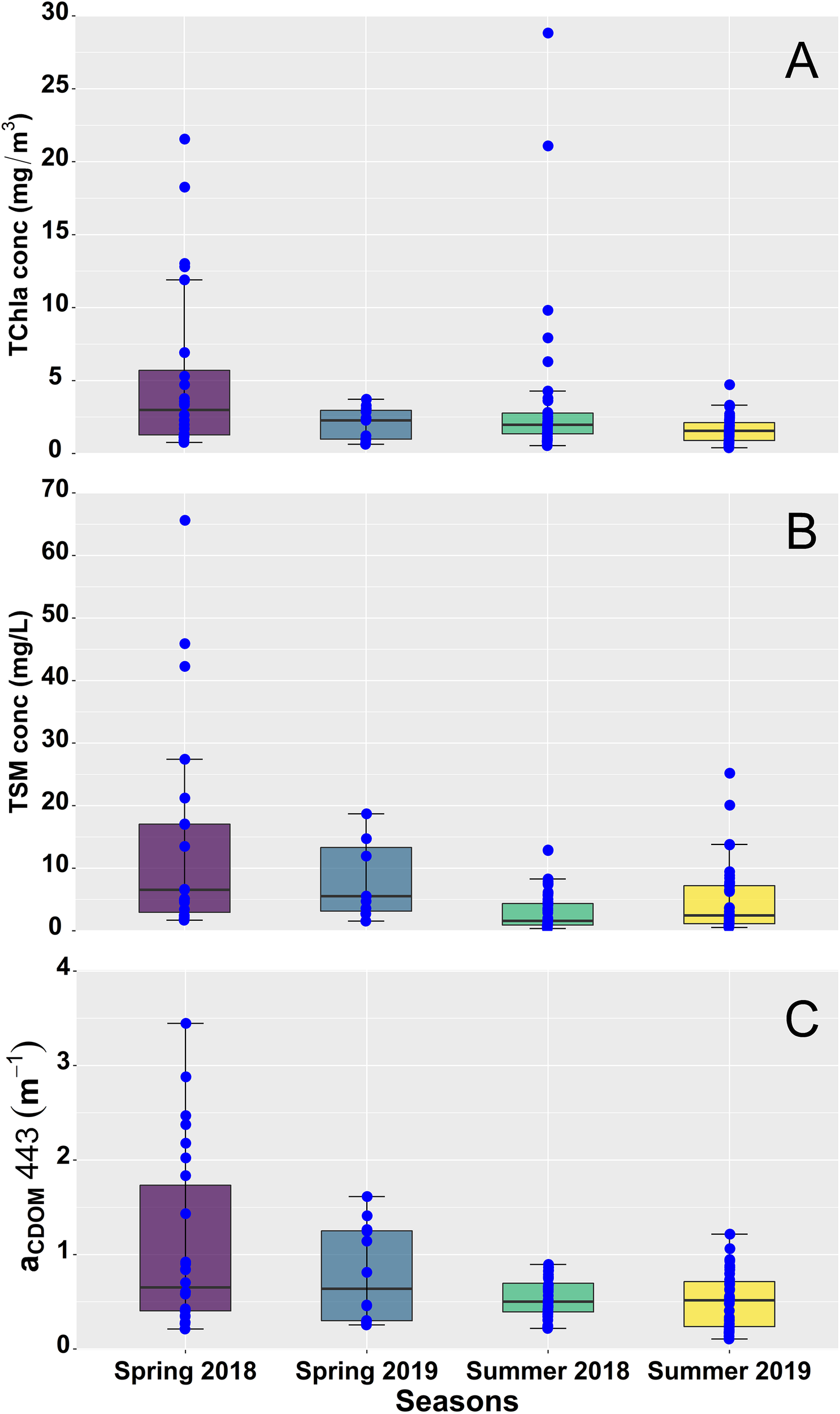
Seasonal variation of (A) total chlorophyll-a concentration (TChla, mg/m3), (B) total suspended matter concentration (TSM, mg/L), and (C) the absorption by colored dissolved organic matter [aCDOM, 443 (m-1] in the Strait of Georgia (SoG) during 2018 and 2019. The upper and lower edge of the box plot represents the first and third quartile, respectively. Outside of the boxes, the whiskers on both quartiles indicate standard error. Blue points represent data points, and points outside the third quartile indicate extreme values.
Surface phytoplankton community composition derived from CHEMTAX for the central SoG (Stn 1 to 5) during 2018 and 2019 is shown in Figure 4. Generally, during spring (March to May) 2018, diatoms dominated the community composition in almost all the stations (54 ± 32%; average ± SD). At this time of the year, the relative contribution of flagellates, including haptophytes, green algae, cryptophytes, dinoflagellates, and dictyochophytes, was low (<14%) and followed by cyanobacteria and raphidophytes (< 7%). A seasonal succession from diatoms to flagellates persisted across the sampling stations during the summer (June to August) of 2018 (Figure 4), when the phytoplankton community composition was highly dominated by raphidophytes (24 ± 23%), followed by green algae (23 ± 10%) and cryptophytes (21 ± 16%). In 2018, high TChla concentration events dominated by raphidophytes were observed towards the western portion of the transect (Station 2) in June and concentrated near the mouth of the Fraser River (Stations 4 and 5) in July. Outside of these events, raphidophyte contributions often persisted through low TChla conditions.
Figure 4
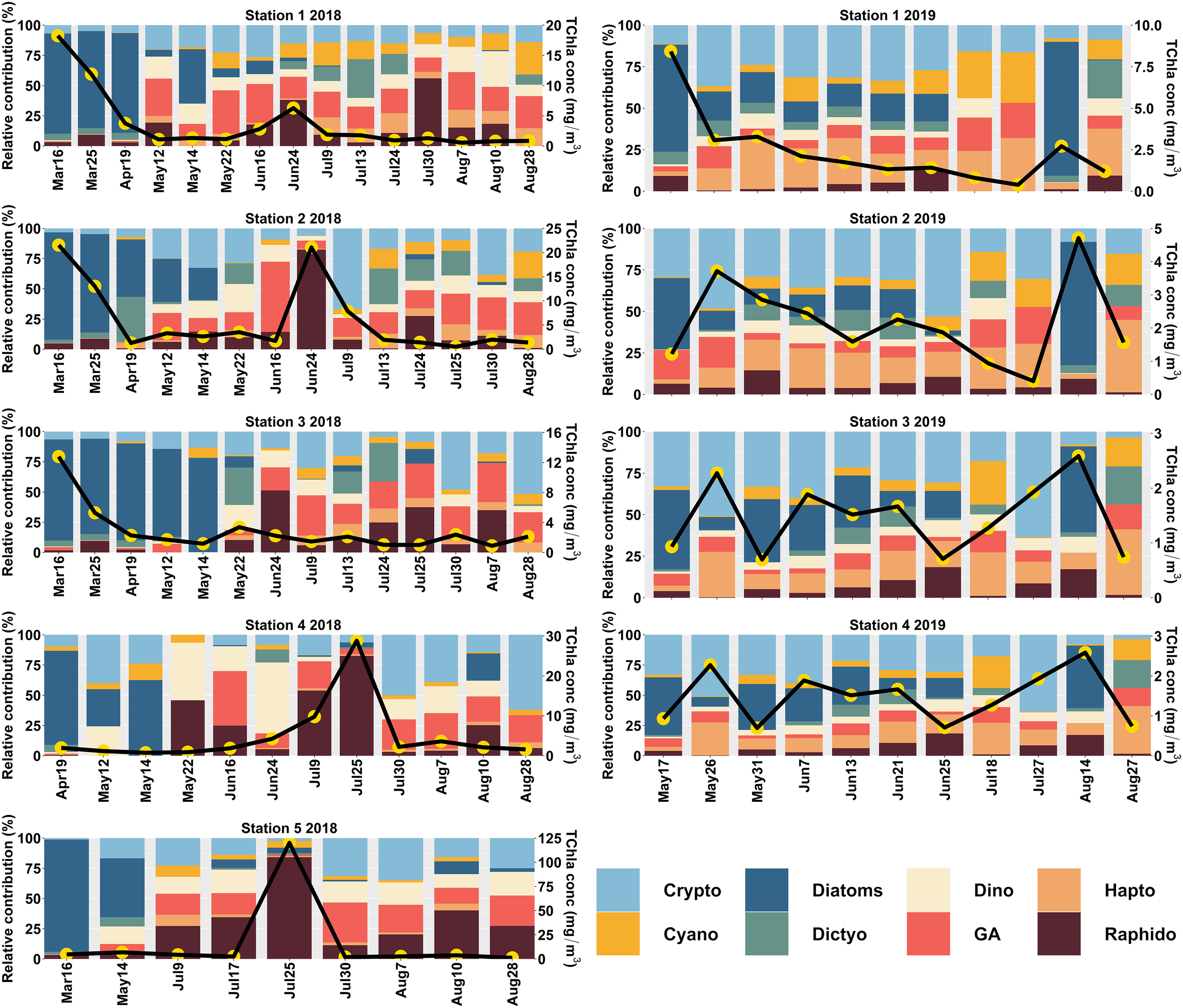
CHEMTAX-derived Phytoplankton Functional Types (PFTs) in the central (Station 1 to 5) Strait of Georgia (SoG) for 2018 and 2019. The primary y-axis shows the relative contribution (%), and the secondary y-axis (black line with yellow circles) indicates the total chlorophyll-a (TChla; mg/m3) concentration.
Unlike the spring of 2018, in 2019, we observed the predominance of cryptophytes (37 ± 13%), followed by diatoms (28 ± 17%). A very similar trend was evident during summer, when cryptophytes (23 ± 16%) and diatoms (22 ± 25%) dominated the community composition, followed by green algae (20 ± 11%). Nevertheless, the relative contribution of other flagellates, such as haptophytes, dinoflagellates, raphidophytes, and dictyochophytes, towards the total phytoplankton concentration was minimal (< 8%). Similar to 2018, raphidophyte contributions were small, but somewhat persistent through low TChla conditions.
In the northern SoG (Figure 5), diatoms were the predominant group at Stn 6 (66 ± 19%) and 7 (24 ± 20%). At station 6, the average contribution of all other groups was minimal (< 18%). In contrast, Stn 7 showed higher contributions from dictyochophytes (17 ± 14%), cryptophytes (17 ± 5%), haptophytes (17 ± 8%), and green algae (16 ± 2%).
Figure 5
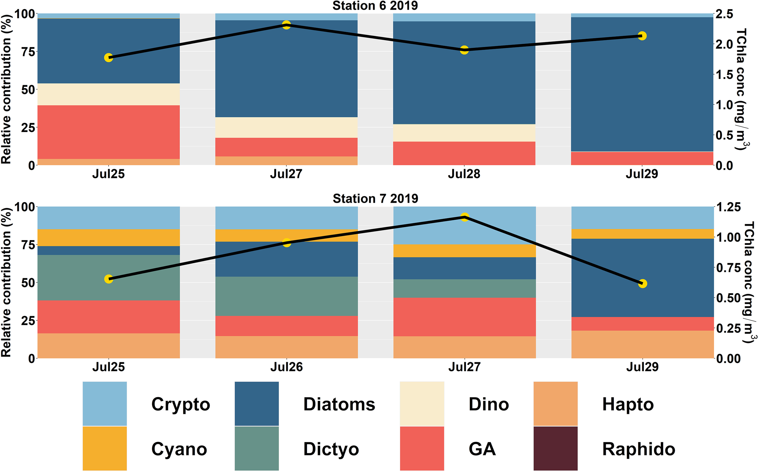
CHEMTAX-derived Phytoplankton Functional Types (PFTs) in the northern (Station 6 to 7) Strait of Georgia (SoG) during 2019. The primary y-axis shows the relative contribution (%), and the secondary y-axis (black line with yellow circles) indicates the total chlorophyll-a (TChla; mg/m3) concentration.
After the spring bloom, a diverse phytoplankton community comprised of flagellates evolved and is summarized by the Shannon-Weaver Index (Supplementary Material 6). In general, the central SoG data showed increased diversity during the summer (1.5 ± 0.3) when diatom contributions were lowest (12 ± 21%). Similarily, in the northern SoG, diversity was higher at Stn 7 (1.6 ± 0.9), which had lower diatom contributions (24 ± 20%) (Supplementary Material 7).
The comparison of the CHEMTAX-derived PFTs with the phytoplankton abundance from microscopy showed significant relationships for diatoms (R2 = 0.87, p< 0.001, n = 8) and dinoflagellates (R2 = 0.52, p<0.05, n = 8). This is an important result that validates the CHEMTAX analysis; however, it is important to note that the sample size for these comparisons was small. Further, pico-sized species likely constituted many of the groups showing high contributions and these would have largely been missed by microscopy and many groups showed low variability in TChla contributions (small dynamic range).
3.2 OLCI derived PFTs
3.2.1 EOF-based analysis of the OLCI Rrs data
The spectral shapes and magnitude of OLCI Rrs and the corresponding standardized Rrs at 10 bands (400, 412, 443, 490, 510, 560, 620, 665, 674, 681 nm) are given in Figure 6. These OLCI Rrs matchup data were then decomposed using SVD to derive nine EOF modes (Table 2), in which the first four modes explained 99.48% of the variance. The spectral distribution of each EOF and the spectral features associated with several seawater constituents are shown in Figure 7. In general, EOF-1 explained 60.33% of the total variability, and exhibited a high reflectance peak at 560 nm and a 680 nm feature likely associated with phytoplankton and TChla fluorescence, respectively. EOF-2 explained 38.33% of the total variability and exhibited a sharp decrease from 500 to 400 nm, indicating the influence of high CDOM absorption in the blue region, and a broad peak from 560 to 700 nm, indicating high backscattering from inorganic suspended sediments. Moreover, EOF-3 explained 0.50% of the variability, showing a decrease in spectral structure from 400 to 450 nm and a spectral peak at 560 and 680 nm. EOF-4 explained only 0.32% of the total variance; however, a trough is evident from 443 to 510 nm likely associated with absorption by different accessory pigments, followed by several peaks at 412, 443, 560, and 681 nm. The spectral peaks observed at 560 and 681 nm could be associated with phytoplankton and TChla fluorescence, respectively. The higher EOFs, such as EOF-5, EOF6, EOF7, EOF8, and EOF9, only showed variance < 0.20%.
Figure 6
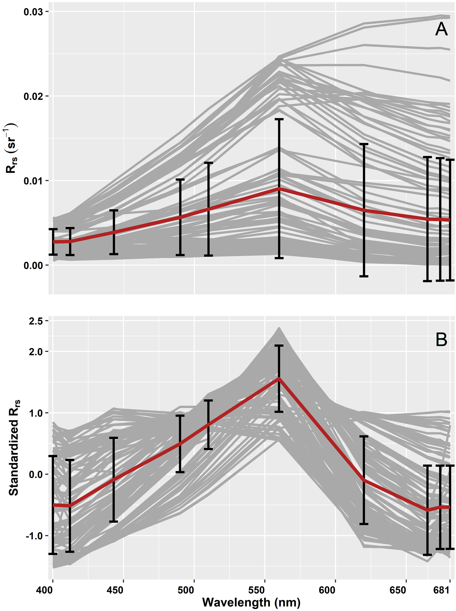
(A) Remote sensing reflectance (Rrs; sr–1(λ)) and (B) corresponding standardized Rrs subjected to the Empirical Orthogonal Function (EOF) analysis. The grey lines show the median spectra from a 3×3 pixel window with the corresponding average spectra in red, and the standard deviation at each band is shown in black.
Table 2
| % of variance | EOF1 | EOF2 | EOF3 | EOF4 | EOF5 | EOF6 | EOF7 | EOF8 | EOF9 |
|---|---|---|---|---|---|---|---|---|---|
| OLCI Rrs | 60.33 | 38.33 | 0.5 | 0.32 | 0.20 | 0.11 | 0.06 | 0.04 | 0.01 |
Percentage of variance explained by Empirical Orthogonal Function (EOF) modes derived from the matchup between Ocean Land Color Instrument (OLCI) remote sensing reflectance [Rrs; sr–1(λ)] and CHEMTAX-derived Phytoplankton Functional Types (PFTs).
This percentage of variance obtained from the matchup between OLCI Rrs and total chlorophyll-a (TChla; mg/m3).
Figure 7
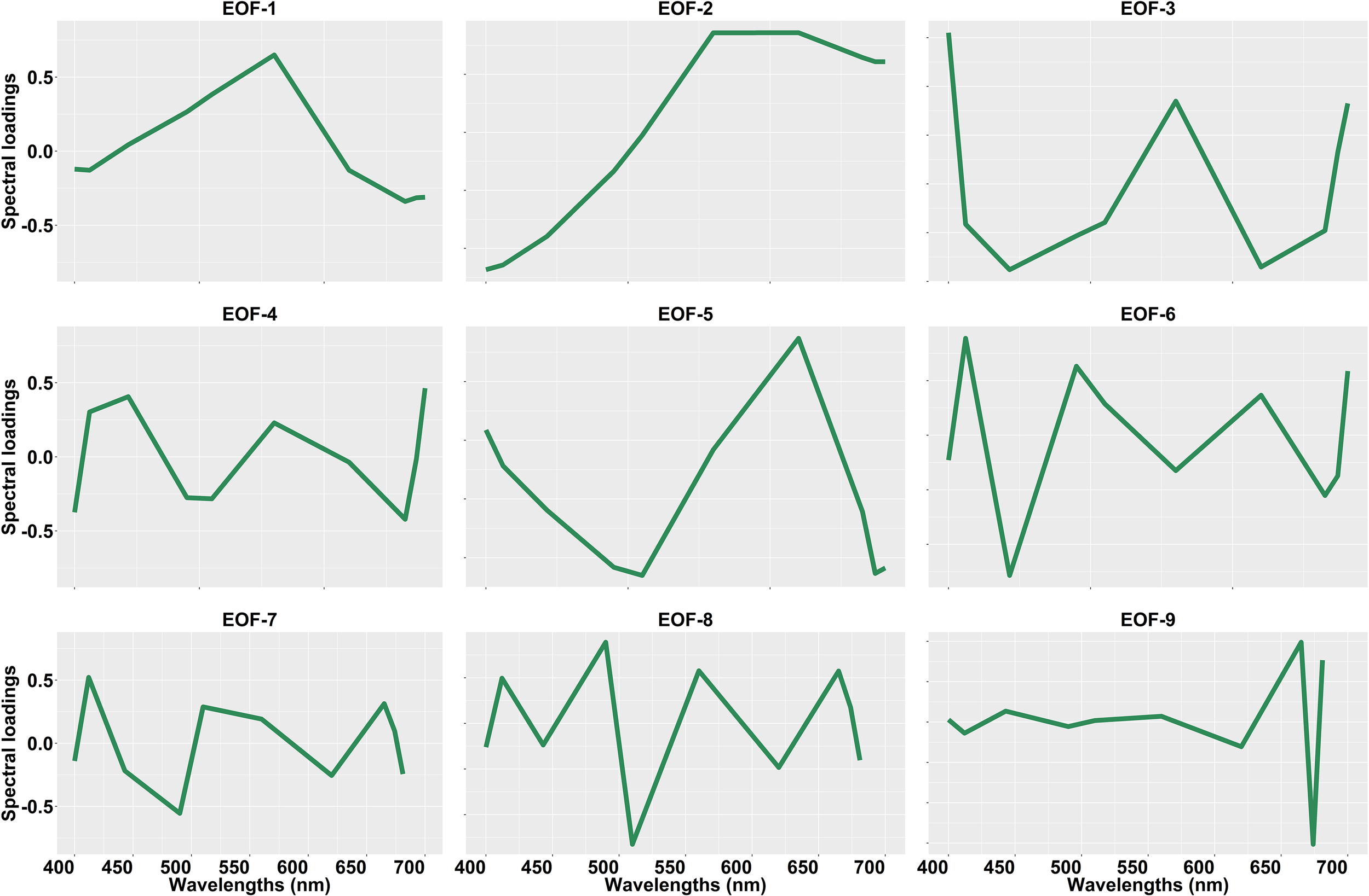
Spectral loadings for the nine Empirical Orthogonal Function (EOF) modes derived from the Ocean Land Color Instrument (OLCI) remote sensing reflectance [Rrs; sr–1(λ)]. This spectral loading was obtained from the matchup between OLCI Rrs and total chlorophyll-a (TChla; mg/m3) concentration.
The ∆AIC (Supplementary Material 8) showed that EOF-4 was the most significant for TChla, diatoms, and dictyochophytes, and higher EOFs were selected for most PFTs (Supplementary Material 8). At the same time, the second most important EOFs differed among PFTs (Supplementary Material 8). For cyanobacteria and dinoflagellates < 3 EOFs were selected to build the regression model (Supplementary Material 8).
3.2.2 Model evaluation
Figure 8 shows the regression between the CHEMTAX-derived PFTs versus TChla concentrations and the Chla concentrations of the eight PFTs retrieved from OLCI. Overall, the regression models showed moderate and highly significant retrieval (p<0.0001) for diatoms and raphidophytes (R2 = 0.45, 0.37, respectively; Table 3). In addition, the regression models for dictyochophytes, haptophytes, green algae, and cryptophytes were also significant (p<0.001; Table 3); however, relatively lower R2 (≤0.30) were observed. Poor performances were observed for dinoflagellates and cyanobacteria (R2 = 0.07, 0.11, respectively; Table 3), with the best performance (R2 = 0.51; p<0.0001) for TChla retrievals. The lowest MDPDs were observed for TChla, green algae, haptophytes, and cyanobacteria (34.26%, 41.18%, 44.18%, 44.29%, respectively), whereas the highest MDPDs were noted for raphidophytes, followed by dinoflagellates (66.78%, 60.27%, respectively; Table 3). MAE was relatively higher for diatoms (MAE = 0.23 mg/m3); however, it was <0.23 mg/m3 for all other PFTs.
Figure 8
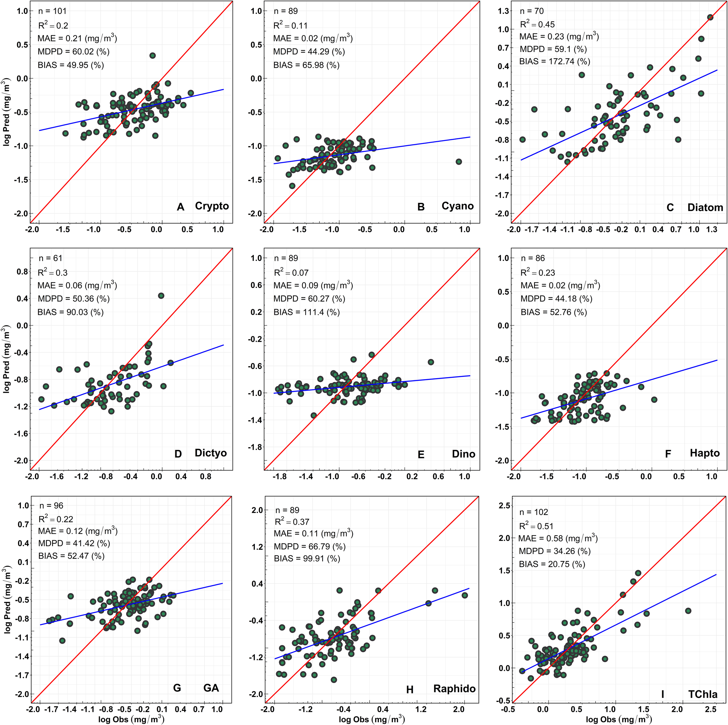
Regression between CHEMTAX-derived (x-axis) versus OLCI-retrieved (y-axis) Chla concentration of (A) Cryptophytes, (B) Cyanobacteria, (C) Diatoms, (D) Dictyochophytes, (E) Dinoflagellates, (F) Haptophytes, (G) Green Algae, (H) Raphidophytes, and (I) total chlorophyll-a (TChla).
Table 3
| N | R2 | MAE | MDPD | Slope | Intercept | R2cv | MAEcv | MDPDcv | p-value | |
|---|---|---|---|---|---|---|---|---|---|---|
| TChla | 102 | 0.51 | 0.58 | 34.26 | 0.51 | 0.34 | 0.43 | 2.76 | 39.12 | 2.2×10⁻¹⁶ |
| Diatoms | 70 | 0.45 | 0.23 | 59.09 | 0.46 | -0.49 | 0.30 | 1.34 | 65.77 | 1.3×10⁻¹⁰ |
| Dictyo | 61 | 0.30 | 0.06 | 50.36 | 0.30 | -1.43 | 0.11 | 0.20 | 61.34 | 4.6×10⁻⁶ |
| Raphido | 89 | 0.37 | 0.11 | 66.78 | 0.37 | -1.13 | 0.25 | 1.90 | 74.17 | 2.2×10⁻¹⁰ |
| Hapto | 86 | 0.23 | 0.02 | 44.18 | 0.23 | -1.96 | 0.14 | 0.07 | 47.13 | 2.9×10⁻⁶ |
| GA | 96 | 0.22 | 0.12 | 41.41 | 0.22 | -1.06 | 0.08 | 0.22 | 49.14 | 1.5×10⁻⁶ |
| Crypto | 101 | 0.20 | 0.21 | 60.02 | 0.20 | -0.85 | 0.10 | 0.46 | 63.54 | 2.2×10⁻⁶ |
| Dino | 89 | 0.07 | 0.09 | 60.27 | 0.07 | -1.93 | 0.00 | 0.17 | 63.25 | 0.01 |
| Cyano | 89 | 0.11 | 0.02 | 44.29 | 0.12 | -2.34 | 0.08 | 0.13 | 48.51 | 0.001 |
Full-fit statistics and Cross-validation statistics derived from the EOF-based algorithm, developed using the matchup between Ocean Land Color Instrument (OLCI) remote sensing reflectance [Rrs; sr–1(λ)] and CHEMTAX-derived Phytoplankton Functional Types (PFTs).
R2, Slope, and Intercept were calculated on a log scale (in natural logarithm), whereas mean absolute error (MAE; mg/m3) and median percentage difference (MDPD; %) were calculated on a non-log scale.
As part of the level-1 evaluation, the robustness of all PFT regression models was further assessed with the cross-validation approach (Table 3). The statistical parameters obtained from the cross-validation procedure were poorer than the entire dataset statistics. For example, a poor R2CV was obtained for almost all PFTs, except TChla (0.43). In general, R2CV ranged from 0 to 0.43 (Table 3). Whereas, MDPDcv ranged from 39.12 to 74.17%, in which the highest MDPDcv was obtained for raphidophytes (MDPD = 74.17%), followed by diatoms (65.77%). However, a low MDPDcv (39.12%) was observed for TChla.
The level-2 evaluation (Figure 9) was conducted for OLCI-derived outputs against the independent Hakai time-series from station QU39 (N = 26, Figure 1). Of the considered groups, green algae, cryptophytes, and diatoms followed similar trends through the Hakai time-series, resulting in significant (p <0.05) retrieval (R2 = 0.33, 0.23, 0.20, MDPD = 163, 46.86, 88.59%, respectively) (Figure 9; Table 4). The best retrieval was noted for TChla, which highly corresponded with the Hakai time-series (R2 = 0.68, MDPD = 52.25%) (Figure 9; Table 4). Except for TChla, diatoms recorded the highest MAE (0.58 mg/m3; Table 4), and MAE for all other groups was < 0.58 mg/m3. The MDPD was the highest for green algae (163%) and raphidophytes (130%), whereas MDPD was relatively lower for cryptophytes (46.86%). Overall, OLCI-derived PFTs, including TChla, over-estimated the lower ranges and under-estimated higher ranges of in situ values. Raphidophytes showed poor correspondence (R2 = 0.08, MDPD = 130%) with the Hakai time-series (Figure 9; Table 4); however, it is important to note that raphidophytes were not observed via microscopy on any of the considered dates, highlighting misclassifications by both CHEMTAX and OLCI-derived outputs under low TChla conditions.
Figure 9
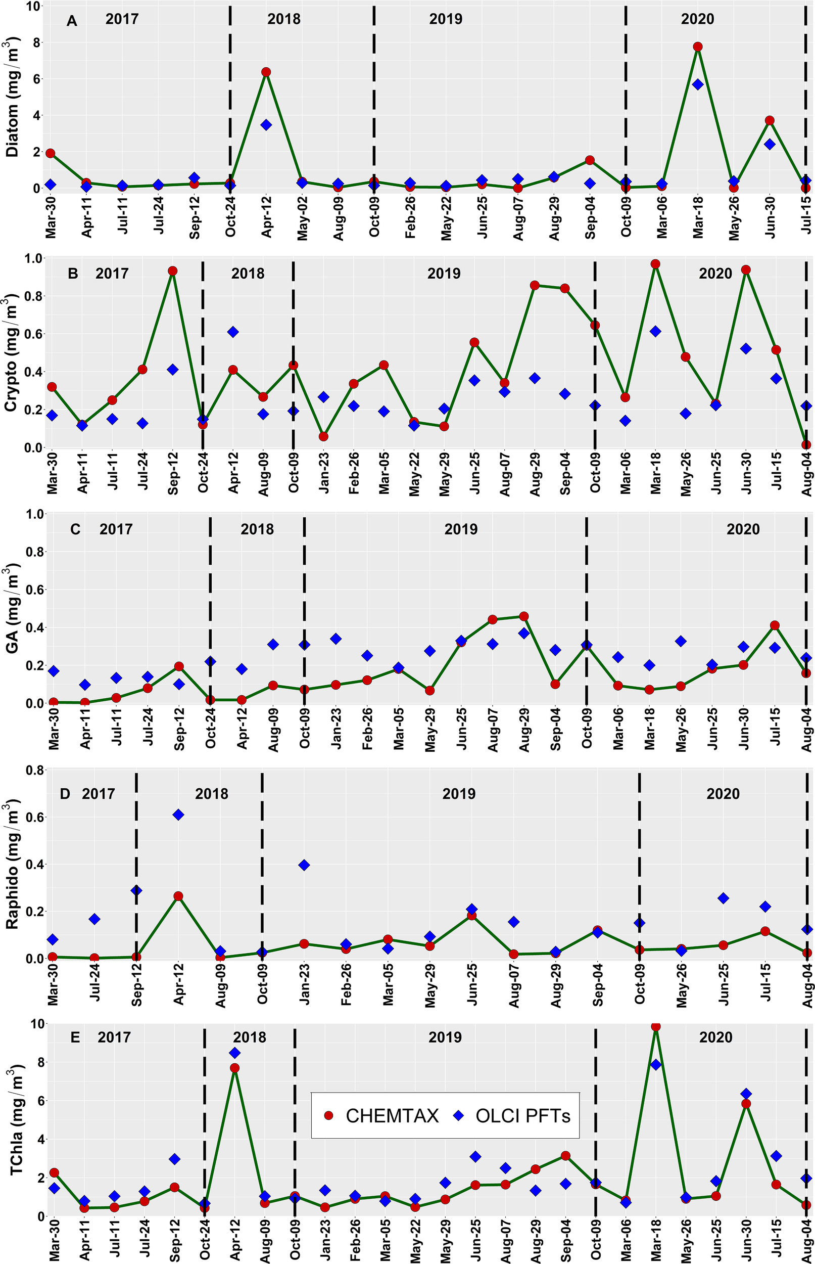
Comparison of the performance of the OLCI-derived (A) Diatoms, (B) Cryptophytes, (C) Green Algae, (D) Raphidophytes, and (E) total chlorophyll-a (TChla) concentration obtained from the daily cloud-free images between spring 2017 to summer 2020 (blue diamonds) against the Hakai time-series data at station QU39 located in the northern Strait of Georgia (SoG) (red circles). The location of station QU39 is given in Figure 1. The vertical lines on each panel separate different years, and note that the matchup data points differ among Phytoplankton Functional Types (PFTs), mainly because all PFT may not be present at all stations. For example, Raphidophytes showed fewer points (19) out of the 26 matchup points, followed by Diatoms (22). Hence, the dates on the x-axis might not be similar for all PFTs.
Table 4
| N | R2 | MAE | MDPD | Slope | Intercept | p-value | |
|---|---|---|---|---|---|---|---|
| TChla | 26 | 0.68 | 0.73 | 52.25 | 0.65 | 0.35 | 2.52×10⁻⁷ |
| Diatoms | 22 | 0.20 | 0.58 | 88.59 | 0.22 | -0.63 | 0.03 |
| Crypto | 26 | 0.23 | 0.21 | 46.86 | 0.23 | -1.18 | 0.01 |
| GA | 25 | 0.33 | 0.12 | 163 | 0.16 | -1.07 | 0.002 |
| Raphido | 19 | 0.08 | 0.10 | 130 | 0.19 | -1.53 | 0.23 |
Validation statistics were obtained from the regression between OLCI-derived Phytoplankton Functional Types (PFTs), including total chlorophyll-a (TChla; mg/m3) versus Hakai time-series data.
R2, slope, and intercept were calculated on a log scale (in natural logarithm), whereas mean absolute error (MAE; mg/m3) and median percentage difference (MDPD; %) were calculated on a non-log scale.
3.3 PFT mapping in SoG from daily OLCI imagery
After the model evaluation, we applied the EOF-based regression algorithm to daily OLCI imagery acquired during cloud-free days between March and September 2018 to provide a qualitative evaluation based on the spatial distribution and seasonal dynamics of PFTs over the SoG. The spatial maps (Figure 10) were produced for diatoms, cryptophytes, green algae, and raphidophytes since they accounted for 74% of the total phytoplankton concentration. Overall, the PFT spatial maps showed a distinct spring and fall bloom in the SoG, which was mostly comparable with the Hakai time-series. During spring, diatoms showed the highest average concentration (avg 5.15 mg/m3) with high concentrations observed near the northern and central SoG, and the Juan de Fuca Strait (Figures 10A1-A2), similar to the Hakai time-series data (diatom Chla ranging from 0.23 to 6.00 mg/m3) in the northern SoG. In comparison, the spatial distribution of cryptophytes and raphidophytes for the spring followed a similar spatial distribution to diatoms, but with relatively lower concentrations (avg 0.70, 1.30 mg/m3, respectively; Figures 10B1-B2, Figures 10D1-D2). Furthermore, the spatial distribution of green algae for the spring showed a comparatively low average concentration (0.32 mg/m3) and tended to show inverse spatial trends to diatoms. Hakai’s data for this week of the year also showed comparable concentrations for cryptophytes, green algae, and raphidophytes in the northern SoG.
Figure 10
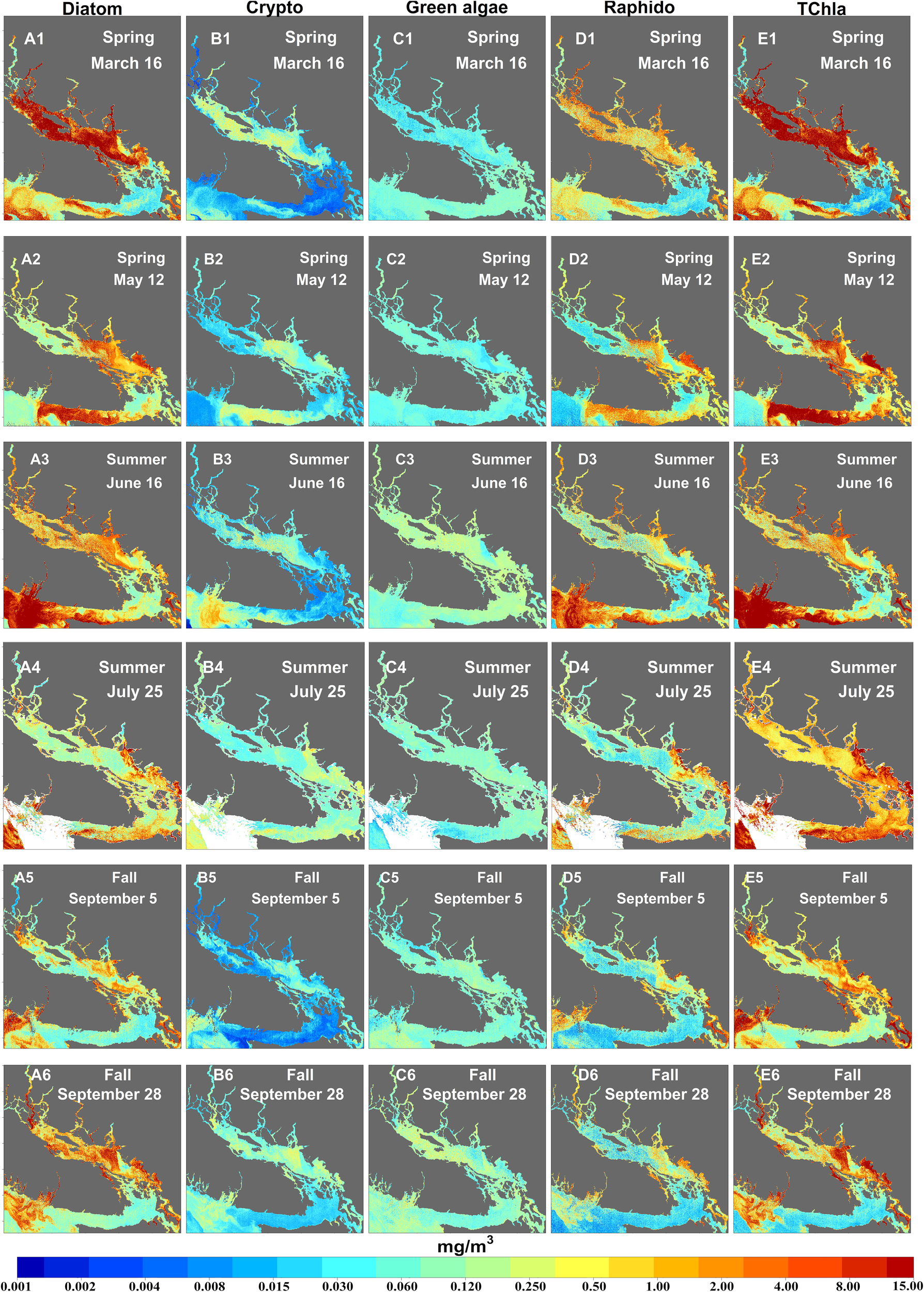
Spatial and seasonal distribution of Diatoms, Cryptophytes, Green Algae, Raphidophytes, and total chlorophyll-a (TChla), retrieved from Ocean Land Color Instrument (OLCI) over the surface waters of the Strait of Georgia (SoG). Only images with >80% coverage were selected for the final map. OLCI imagery was acquired on cloud-free days from spring to fall of 2018, and the specific days were given in the spatial map. White regions in the maps show the clouds.
Following the spring period, the summer average diatom concentration decreased (4.37 mg/m3), but strong diatom bloom events were still observed off of the southwestern coast of Vancouver Island, with patches of high contributions in the central and northern SoG near the beginning of summer (June 16th – Figure10-A3). By July 25th, diatom contributions had decreased considerably (Figure10-A4). Consistent with these observations, Hakai’s data for a similar period showed low diatom concentrations in the northern SoG, ranging from 0.12 to 0.14 mg/m3. Furthermore, comparable with the Hakai time-series, OLCI-derived green algae showed a relatively higher average concentration (0.37 mg/m3; Figure 10-C3) than spring with localized areas of high cryptophyte concentrations in the central SoG and Juan de Fuca Strait (Figure 10-B3). Interestingly, raphidophytes recorded the highest average concentration during the summer (2.24 mg/m3), and blooms were observed off the southwest coast of Vancouver Island and close to the Fraser River mouth (Figures 10-D3, 10-D4). Of note, on June 16th, both diatoms and raphidophytes showed high concentrations off of the southwest coast of Vancouver Island; however, concentrations between the two groups was decoupled within the central and northern SoG, where diatom concentrations were high, and raphidophyte contributions were low. Finally, in fall, diatoms still constituted the highest average concentration (1.35 mg/m3), especially near the central and northern SoG and off the south of Vancouver Island (Figure 10-A6). During this season and, similar to the Hakai time-series, the spatial distribution of cryptophytes was similar to the distribution of diatoms but with a relatively low average concentration (0.49 mg/m3). In turn, green algae showed relatively high concentrations in the central and northern SoG and off of southern Vancouver Island (Figure 10-C6) resulting in the highest average seasonal concentration (0.41 mg/m3) for this PFT. Overall, TChla showed high concentrations throughout the season with high concentration regions localized in the central and northern SoG, near the mouth of the Fraser River, within the Juan de Fuca Strait, and off the south coast of Vancouver Island (Figures 10-E1, 10-E2, 10-E3, 10-E4, 10-E5, 10-E6).
4 Discussion
4.1 EOF-based PFT retrievals and source of uncertainties
EOF analysis has successfully been used to derive phytoplankton cell abundance and the concentration of accessory pigments and multiple PFTs from the global open ocean and regional waters (e.g., Craig et al., 2012; Bracher et al., 2015; Lange et al., 2020; Xi et al., 2020); however, few of these studies have addressed coastal Case-2 waters (e.g., Craig et al., 2012). In these waters, the relationship between EOFs to specific PFTs can be hindered by high concentrations of water constituents such as CDOM, detritus, and TSM, which can largely define the reflectance spectra and mask PFT signals (Mouw and Yoder, 2010; Craig et al., 2012; Mouw et al., 2017). In this study, high variability of these constituents were observed (Table 1), thus significantly contributing to the reflectance signal and EOF modes (Figure 7), as observed in Phillips and Costa (2017) and Craig et al. (2012). Furthermore, EOF modes from oceanic waters (Bracher et al., 2015; Xi et al., 2020) show high dissimilarity to those found in this study, likely due to the absence of high concentrations of non-phytoplankton constituents. As a result, the derivation of PFTs in this study was likely hindered by the high bio-optical complexity characteristic of the SoG (Loos and Costa, 2010; Loos et al., 2017; Phillips and Costa, 2017; Giannini et al., 2021). This difficulty would have been most pronounced for low biomass groups which showed weak signals.
Beyond the inherent role of the Case-2 waters’ different optical constituents on the EOF retrievals, the biomass contribution of a specific PFT to the total phytoplankton biomass is known to be relevant for accurate PFT retrievals from spectral data. Of the two levels of validation, the first validation showed good retrievals for diatoms and raphidophytes, and the second validation showed that green algae, cryptophytes, and diatoms followed the seasonal trends of their corresponding in situ values from a high temporal resolution Hakai time-series (Figure 9). This is likely associated with their larger contribution (62%) to the total concentration, as demonstrated in the CHEMTAX model output (Figure 4). These results are encouraging with regard to the remote sensing of PFTs over optically complex Case-2 waters, where previous studies have documented that PFT retrieval over Case-2 waters is challenging (Craig et al., 2012; IOCCG, 2014; Mouw et al., 2017). At the same time, the poorest retrievals obtained for haptophytes, dictyochophytes, cyanobacteria, and dinoflagellates was likely related to their low concentration (26%), resulting in low contributions to the Rrs signal. Similarly, Xi et al. (2020) also observed poor performance for low biomass prokaryotes (R2cv = 0.11; MDPDcv = 55.08%) and Prochlorococcus (R2cv = 0.18; MDPDcv = 42.68%), and Bracher et al. (2015) showed slightly poorer retrievals (R2cv = 0.28; MDPD = 31%) for the pigment zeaxanthin (found in low concentrations), a diagnostic pigment for cyanobacteria.
Other factors, such as the quantity and quality of in situ and satellite matchup data also impact the performance of satellite-derived PFTs. For the EOF-based PFT algorithm, the number of matchup data points and their representation of the range of phytoplankton groups in the region are crucial to enhance the accuracy of the retrievals (Bracher et al., 2015; Xi et al., 2020). Bracher et al. (2015) suggested that at least 50 valid matchup data points are necessary for statistically significant pigment estimation, specifically for open ocean waters. Xi et al. (2020) employed a larger number of matchup data points (52-394) for global open ocean waters, with an even higher number (483) in a more recent publication (Xi et al., 2021). Lange et al. (2020) employed 73-78 matchup points to develop an EOF-based algorithm to retrieve phytoplankton cell abundance from MODIS across the Atlantic Ocean. However, Craig et al. (2012) showed that a reliable EOF-hyperspectral-based model could be built with 15 valid data points, specifically for one season and at a local scale. In our study, the total number of matchup data points was between 61 and 102, which is within the range suggested by the above authors. However, given the optical complexity of our waters, a higher number of matchups would likely improve the PFT retrievals.
The spatial and temporal variability of the matchup samples, which has implications on data quality, is also an important factor in evaluating the EOF-based PFT retrievals, especially in Case-2 dynamic coastal waters such as the SoG. This is a common problem in validating satellite-derived products of coastal waters (e.g., Mahadevan and Campbell, 2002; Moses et al., 2016; Barnes et al., 2019; Tilstone et al., 2022). Specifically in the SoG, Nasiha et al. (2022) have shown large spatial variability of in situ above-water reflectance within the 300m spatial resolution of OLCI. Notably, most of this variability was observed at the frontal region of the Fraser River and within transitional oceanic waters and likely has considerable implications on the quality of in situ data for satellite validation purposes. Further, Giannini et al. (2021) have shown the importance of the temporal mismatch between in situ and OLCI data in the SoG due to the dynamic nature of this water system. Here, an attempt was made to reduce these spatial issues by rejecting matchups corresponding to transitional waters, and further, to minimize temporal mismatch by relocating the sample’s position using surface current maps generated using a CODAR system (Halverson and Pawlowicz, 2016). This method was successfully adopted by Giannini et al. (2021). Out of the 102 matchup samples utilized in this study, 20 were successfully relocated using the surface current map. Indeed, after the relocation, we observed improved performance in the Rrs matchup analysis (not shown). However, it is still challenging to detect and quantify any remaining source of uncertainties associated with this spatial and temporal water mass mismatch.
Uncertainties associated with CHEMTAX model outputs should also be considered in evaluating the EOF-based PFT retrievals. For example, CHEMTAX outputs are more prone to errors in environments with complex phytoplankton community composition, notably when local ratios are unknown, and many species have similar pigment composition (Lewitus et al., 2005); this resembles some of the conditions in the Salish Sea. For instance, the haptophyte, Phaeocystis pouchetti, has been shown to periodically lack 19′-hexanoyloxyfucoxanthin (19HF) and have relatively high 19′-butanoyloxyfucoxanthin (19BF) concentrations; in these conditions, the utilized CHEMTAX ratios may result in misclassification of the haptophyte as a dictyochophyte (Del Bel Belluz et al., 2021). In addition, raphidophytes, such as Heterosigma akashiwo, often bloom regionally and have similar pigment ratios to diatoms, with the separation of raphidophytes dependent on their high violaxanthin to TChla ratios. However, violaxanthin concentrations are variable and broadly present among groups (Lewitus et al., 2005; Laza-Martinez et al., 2007; Higgins et al., 2011). In this study, violaxanthin to TChla ratios were noticeably high during raphidophyte blooms, and CHEMTAX appeared to be able to distinguish these events. Yet, under lower TChla concentration conditions, raphidophyte contributions often persisted, likely representing misclassifications and underestimations of other groups. These misclassifications are evidenced by the small CHEMTAX and satellite-based raphidophyte contributions shown over the Hakai time-series comparison (Figure 9); no raphidophytes were observed via microscopy during much of this time-series (Del Bel Belluz et al., 2021). As such, errors from CHEMTAX may have been perpetuated to the satellite models.
To address this issue, novel “data driven” approaches have been developed to help account for PFTs present in low contributions and also, to deal with issues in CHEMTAX analysis such as misclassifications of groups with similar pigment profiles and pigment collinearity (Catlett and Siegel, 2018; Kramer and Siegel, 2019; Kramer et al., 2020). These approaches, which are not hindered by co-correlation between pigments, use both cluster and EOF analysis to group species with similar pigment ratios. Outputs from these methods typically have fewer PFT groups (< 5) that combine communities that covary in the environment. Using the same clustering methods, the pigment data in this study clustered into 4 pigment groups: diatoms, dinoflagellates, haptophytes/pelagophytes, and green algae/cryptophytes/cyanobacteria (Supplementary Material 9). The use of this more generalized approach in our study may have allowed for a more accurate retrieval of a broad “small flagellate” group during high diversity low TChla summer conditions, similar to those used effectively by regional particulate fatty acid studies (Costalago et al., 2020; McLaskey et al., 2022). However, the results of this clustering approach grouped violaxanthin with green algae pigments suggesting that this group drove its variability, which is generally the case under non-raphidophyte bloom conditions. As a result, this approach would not have allowed for the separation of raphidophytes, a toxic species with considerable regional impacts on fish (Esenkulova et al., 2021), but likely helps explain the misclassifications described above.
In order to fully assess the above error and decide on the best approaches, independent validation of in situ pigment-based PFT results are needed: this is a major shortcoming of many pigment-based studies (e.g., Chase et al., 2020; Kramer et al., 2020). In our study, regional CHEMTAX results corresponded well with expected trends in phytoplankton communities (discussed below), qualitative microscopy comparisons (Del Bel Belluz et al., 2021), and particulate matter fatty acids and size-fractionated Chla (SF-Chla) (Costalago et al., 2020; McLaskey et al., 2022); however, no direct cross comparisons have yet been performed. This lack of comparison is partially due to the difficulty in comparing pigment-based approaches with other measures of phytoplankton composition (Higgins et al., 2011). In particular, microscopy is skewed to larger species and cannot resolve pico-sized species known to often dominate summer conditions in the SoG (Del Bel Belluz et al., 2021). This trend is evidenced by the small and limited CHEMTAX validation dataset used here, which showed correspondence with only more easily preserved diatoms. Additional sources of validation, using flow cytometry, size-fractionated filtration (SFF), conventional imaging flow cytometry (Olson and Sosik, 2007), Imaging FlowCytobot, genomics, and next-generation sequencing (see IOCCG, 2014 and Lombard et al., 2019 for a detailed review) are needed to evaluate pigment-based community methods and satellite outputs.
Finally, the quality of atmospheric correction and its effect on the OLCI-measured signal is a consideration in evaluating the EOF-based PFT retrievals. For oligotrophic oceanic gyre waters, Rrs uncertainties in blue wavelengths are above 5% (Hu et al., 2013), and are even higher in optically complex waters (Moore et al., 2015). A recent study by Giannini et al. (2021) assessed the radiometric qualities of OLCI Rrs in northeast Pacific coastal waters, showing the highest errors associated with the blue bands (400, 412, 443 nm) when compared with autonomous above-water in situ reflectance measurements (Wang and Costa, 2022). A significant Rrs underestimate in the blue and red bands of OLCI was also reported in the European coastal and inland waters (Zibordi et al., 2018; Bi et al., 2018; Li et al., 2019; Alikas et al., 2020; Shen et al., 2020; Vanhellemont and Ruddick, 2021). Although POLYMER has been proven to outperform other methods to retrieve OLCI Rrs for the coastal waters of BC, Giannini et al. (2021) argue that uncertainties exist and are likely associated with the optimization of the model, which considers TChla and a coefficient (fb) that scales the particulate backscattering in the water column, but does not consider the contribution of CDOM (Steinmetz et al., 2016). As previously discussed, CDOM is a significant optical constituent affecting the light spectra in the SoG (Loos and Costa, 2010; Phillips and Costa, 2017, Table 1), with aCDOM in our study ranging from 0.11 to 3.45 m–1 (Table 1). Since the launch of the Sentinel 3A, the uncertainties found between the products derived from OLCI using different processing approaches, especially for coastal waters, have been under critical evaluation and are still an active area of research (e.g., Zibordi et al., 2018; Hieronymi, 2019; Mograne et al., 2019; Gossn et al., 2019; Giannini et al., 2021; Vanhellemont and Ruddick, 2021; Tilstone et al., 2021).
4.2 Dynamics of PFTs in the SoG
The OLCI-derived PFT maps showed strong spring diatom blooms with the highest concentrations observed in the central and northern SoG (Figure 10-A1). These findings are in-line with TChla concentrations and CHEMTAX, which showed that diatoms dominated the phytoplankton community in the spring of 2018 (Figure 4). For the same period, in situ observations (microscopy, CHEMTAX, particulate matter fatty acids, and SF-Chla) collected across the SoG showed a similar spring bloom timing with the community dominated by the centric diatoms Thalassiosira, Skeletonema, and Chaetoceros (Nemcek et al., 2018; Del Bel Belluz et al., 2021; Esenkulova et al., 2021; McLaskey et al., 2022). In the SoG, diatom-dominated spring blooms are well documented in the literature (e.g., Harrison et al., 1983; Allen and Wolfe, 2013; Suchy et al., 2019; Del Bel Belluz et al., 2021). As in many temperate systems, diatoms are the primary group that quickly respond to increased nutrient and light conditions resulting in rapid accumulation and bloom conditions (Allen and Wolfe, 2013). Both satellite-derived time-series data (Suchy et al., 2019) and coupled-biophysical model results (Collins et al., 2009) have shown that spring bloom timing and strength are related to early water column stratification due to positive anomalies in SST, Fraser River discharge, and reduced wind stress. These conditions promote the relatively high average surface TChla concentration in the SoG, which is one of the most productive regions on the west coast of North America (Jackson et al., 2015).
During summer, EOF-based PFT retrievals generally showed reduced TChla concentrations and diatom contributions, with exception to localized events off of the southwest coast of Vancouver Island and in the central and southern SoG. Furthermore, the northern SoG typically showed reduced TChla and diatom contributions compared to the central and southern regions (Figures 10-A4, 10-E4). This succession to lower concentration summer conditions is expected for the region. For instance, a monthly climatology of satellite-derived surface TChla over 13 years (2003 to 2016) showed relatively lower TChla during summer and reduced concentrations focused in the northern SoG (Suchy et al., 2019). Spatially, the northern SoG is more stable and stratified and prone to limiting nitrate concentrations, whereas the southern SoG is exposed to higher vertical mixing bringing nutrient-rich water from the subsurface to the sunlit layer (Peña et al., 2016). In contrast, higher phytoplankton concentrations found to the south of Vancouver Island have been linked to wind-induced seasonal upwelling, freshwater discharge from Fraser and Columbia Rivers, and the outflow of nutrient-rich low salinity water from the Juan de Fuca Strait (Masson and Cummins, 2000; Hickey and Banas, 2008; Thomson et al., 2014). Indeed, the brackish water outflow from the Juan de Fuca Strait is a significant source of nitrate to the continental shelf of Vancouver Island and northern California Current (Foreman et al., 2008; Hickey and Banas, 2008). These nutrient-rich waters supply adequate nitrate concentration to the mixed layer depth promoting increased phytoplankton biomass and primary productivity to the southwest of Vancouver Island during summer (MacFadyen and Hickey, 2010).
The summer succession to flagellate-dominated communities in the SoG was apparent in the in situ CHEMTAX model output and less so in the OLCI-derived spatial maps. In agreement with our observations, many authors using a variety of approaches have reported a similar seasonal succession from diatoms to small flagellates and noted that the northern SoG has a more diverse flagellate dominated community when compared to the central SoG (e.g., Harrison et al., 1983; Haigh and Taylor, 1991; Del Bel Belluz et al., 2021; McLaskey et al., 2022). The Shannon-Weaver Index calculated from our CHEMTAX model output supports the literature showing higher diversity in the summer when small flagellates were dominant (such as green algae and cryptophytes, followed by dinoflagellates, haptophytes, and dictyochophytes), and relatively higher diversity in the northern SoG than the central SoG (Supplementary Material 7).
The strong raphidophyte blooms observed in summer 2018 were an exception to the seasonal succession to a diverse range of small flagellates. These blooms were observed by multiple other studies in the region (Nemcek et al., 2018; Pawlowicz et al., 2020). In particular, Esenkulova et al. (2021) found June and July 2018 to be an exceptional year in terms of Heterosigma akashiwo, with abundance reaching 11,000 cells mL-1, compared to data from 2015-2017 (150 cell mL-1). Similar to the results of this study, these authors showed that in the SoG, Heterosigma akashiwo are typically observed from May to September, with the summer 2018 blooms having a distinct spatial distribution concentrated near the Fraser River mouth (Figure 10 D4). The location of these blooms near the Fraser River suggests that Heterosigma akashiwo is strongly associated with highly stratified low salinity waters with low nitrate and phosphate concentrations and high silicate concentrations (Esenkulova et al., 2021). In addition, and similar to the results of this study, Heterosigma akashiwo was observed off of the southwest coast of Vancouver Island (Figure 10-D3) on June 16th, 2018 by Gower and King (2018) using the Maximum Chlorophyll Index (MCI) method on satellite imagery and these results were corroborated with microscopy. In the SoG, Heterosigma akashiwo are thought to have negative impacts on wild Pacific salmon populations and significantly impact the fin-fish and salmon aquaculture industries driving large fish kill events (Rensel et al., 2010; Haigh and Esenkulova, 2014). As a result, the ability to monitor these species using EOF-based PFT maps would provide a mechanism for better understanding and mitigating the negative effects of these harmful species.
Lastly, a fall bloom dominated by diatoms is evident in our spatial maps, which is typical for this region (Nemcek et al., 2018; Del Bel Belluz et al., 2021). This bloom was largely constituted by Pseudo-nitzschia and was observed spanning much of the northern SoG (Nemcek et al., 2018; Esenkulova et al., 2021; Del Bel Belluz et al., 2021). On a broader temporal scale, Jackson et al. (2015); Peña and Nemcek (2018), and Suchy et al. (2019) have reported fall blooms on the Vancouver Island coast. Generally, the primary driver for the 2018 fall bloom in the SoG was the reintroduction of nutrients into the sunlit layer following high summer stratification and grazing (Del Bel Belluz et al., 2021). In turn, autumn blooms to the south of Vancouver Island have been attributed to the seasonal wind-induced upwelling followed by freshwater discharge from the Columbia River or Fraser River and the nutrient-rich water outflow from the Juan de Fuca Strait (Jackson et al., 2015).
5 Conclusion and outlook
This is the first study to characterize the spatial-temporal dynamics of the major PFTs in the SoG, an optically complex Case-2 system on the west coast of Canada, with satellite data using an EOF-based algorithm combined with CHEMTAX model outputs. As a result of the complexity of these waters, many of the low concentration groups such as haptophytes, dictyochophytes, dinoflagellates, and cyanobacteria showed poor performance. However, the first level of validation demonstrated reliable performance for diatoms and raphidophytes, and the second level of validation with an independent Hakai time-series showed the best retrieval for TChla and green algae, cryptophytes, and diatoms showed similar seasonal trends as their corresponding in situ values. In this comparison, raphidophyte outputs by both CHEMTAX and satellite retrievals suggested misclassifications during the observed non-raphidophyte bloom conditions over the Hakai time-series when no raphidophytes were observed via microscopy.
Qualitative validations of the spatial-temporal 2018 EOF-based PFT generally agreed with expected patterns for this region with strong spring bloom highly dominated by diatoms, and primarily located in the central and northern SoG and Juan de Fuca Strait. During summer, diatoms showed high concentration off of the southwest coast of Vancouver Island and in patchy regions within the central SoG. As expected based on regional studies, summer TChla and diatom contributions decreased with the lowest contributions observed towards the northern SoG. In turn, patches of increased cryptophyte contributions were noticeable in the central SoG and Juan de Fuca Strait from spring through summer. Green algae, which generally shows its highest concentrations in the summer through autumn, showed low concentrations during spring throughout the central and northern SoG. Furthermore, similar to the CHEMTAX model output and literature, the EOF-based PFT maps revealed 2018 summer raphidophyte blooms (Heterosigma akashiwo) off of the southwest coast of Vancouver Island, within the Juan de Fuca Strait and close to the Fraser River mouth. Finally, a fall bloom was evident in our spatial maps in which diatoms displayed high concentration near the central and northern SoG and south of Vancouver Island. Overall, diatoms demonstrated high average concentrations throughout the study period, and relatively low average concentrations were observed from green algae, cryptophytes, and raphidophytes.
The results of this study suggest that retrieving PFTs in the SoG is highly challenging, likely as a result of the strong contributions of CDOM and particulate suspended matter to the satellite-measured reflectance signal. Further work is required to improve the algorithm and should rely on the following: better sensor vicarious calibration and atmospheric correction of the measured radiance signal; considerations of in situ data quality, including analytical errors; use of broader data-driven pigment methods and quantitative in situ validation utilizing a variety of methods; representation of the phytoplankton group’s dynamic range, and; improving the spatial-temporal quality of the matchups. Also, considering that the retrieval algorithm is an emerging technique, further research is necessary to investigate the over-estimation of the lower ranges and under-estimation of higher ranges of PFT Chla, and to promote the introduction of non-linear fitting in the regression model. Finally, another limitation of our EOF-based PFT analysis is the lack of estimation of per-pixel uncertainty, which to our knowledge has only been reported by Brewin et al. (2017) and Xi et al. (2021). In our study, we used OLCI Rrs as the spectral input data derived through the POLYMER algorithm, and the uncertainty for the POLYMER derived Rrs is currently under development (Steinmetz, personal communication). Hence, performing per-pixel uncertainty of our OLCI-derived PFTs is currently not feasible. Besides, the advance of POLYMER is still an ongoing field, so future studies that aim to elucidate PFTs using POLYMER Rrs should be able to justify the per-pixel uncertainty estimates of PFTs using an updated version of POLYMER, especially over coastal waters.
Despite the shortcomings and uncertainties of our satellite product, our study shows the potential of OLCI for deriving major PFTs over a large spatiotemporal scale, which are not achievable via ship-based measurements. With continued research, the methods deployed here will greatly help to further our understanding of phytoplankton dynamics in complex coastal regions such as SoG and aid in the management of critical species such as migrating Pacific Salmon.
Funding
This research was funded by NSERC NCE MEOPAR - Marine Environmental Observation, Prediction and Response Network; Canadian Space Agency (FAST 18FAVICB09). Additional support from CFI/BCKDF and NSERC-DG to Costa for instruments on the BC Ferry. Hongyan Xi’s and Astrid Bracher’s contributions were funded by the ESA S5P+Innovation Theme 7 Ocean Color (S5POC) project (No 4000127533/19/I-NS) and by the Copernicus Marine Service GLOPHYTS project (21036L05B-COP-INNO SCI-9000). Copernicus Marine Service is implemented by Mercator Ocean in the framework of a delegation agreement with the European Union.
Acknowledgments
The authors would like to thank the Spectral lab members, especially Dr. Giannini, who organized and participated in the fieldwork. We acknowledge the BC Ferries Corporation for their permission for their crew members’ technical support during the fieldwork. The authors also thank ONC (Ocean Network Canada) for their technical help with FOCOS (Ferry Ocean Color Observation Systems) and ferrybox data acquisition. We thank Hakai Institute for providing data for the validation of PFTs retrieved from OLCI imagery. We also acknowledge Cermaq, Canada, for providing the opportunity to conduct fieldwork in their aquaculture farms, logistical support, and help with fieldwork. Finally, the authors thank Keith Holmes for his help with graphics.
Publisher’s note
All claims expressed in this article are solely those of the authors and do not necessarily represent those of their affiliated organizations, or those of the publisher, the editors and the reviewers. Any product that may be evaluated in this article, or claim that may be made by its manufacturer, is not guaranteed or endorsed by the publisher.
Statements
Data availability statement
All analysis and model establishment were performed with R programming. The core functions used in the EOF model training part (Figure 2) in section 2.3 steps 1-2 are `SVD' (singular value decomposition) for EOF analysis, `GLM' (generalized linear models) for multilinear regression between EOF modes and PFTs, and `step' for the stepwise routine to remove insignificant predicting terms. The numeric matrices of V ∙ Λ-1 and the regression coefficients determined by the training part were used for the EOF model applications, and they are provided in Supplementary Materials 10 and 11. The R script on the model application procedure to estimate different PFT Chla is available at https://github.com/vishnu-star/Mapping-Phytoplankton-Functional-Types.git. The in situ and satellite data are presented in the article/Supplementary Materials, and further inquiries can be directed to the corresponding author.
Author contributions
PS: Conceptualization, data collection, analysis, methodology, figure preparation, and writing of the manuscript. HX: methodology, reviewing, and editing. JB: methodology, writing, reviewing, and editing. MH: methodology. AB: methodology, reviewing, and editing. MC: conceptualization, methodology, reviewing, and editing. All authors contributed to the article and approved the submitted version.
Conflict of interest
The authors declare that the research was conducted in the absence of any commercial or financial relationships that could be construed as a potential conflict of interest.
Supplementary material
The Supplementary Material for this article can be found online at: https://www.frontiersin.org/articles/10.3389/fmars.2022.1018510/full#supplementary-material
References
1
Alikas K. Ansko I. Vabson V. Ansper A. Kangro K. Uudeberg K. et al . (2020). Consistency of radiometric satellite data over lakes and coastal waters with local field measurements. Remote Sens.12, 1–34. doi: 10.3390/rs12040616
2
Allen S. E. Wolfe M. A. (2013). Hindcast of the timing of the spring phytoplankton bloom in the strait of Georgia 1968-2010. Prog. Oceanogr.115, 6–13. doi: 10.1016/j.pocean.2013.05.026
3
Alvain S. Moulin C. Dandonneau Y. Bréon F. M. (2005). Remote sensing of phytoplankton groups in case 1 waters from global SeaWiFS imagery. Deep. Res. Part I. Oceanogr. Res. Pap.52, 1989–2004. doi: 10.1016/j.dsr.2005.06.015
4
Armbrecht L. H. Wright S. W. Petocz P. Armand L. K. (2015). A new approach to testing the agreement of two phytoplankton quantification techniques: Microscopy and CHEMTAX. Limnol. Oceanogr. Methods13, 425–437. doi: 10.1002/lom3.10037
5
Bailey S. W. Werdell P. J. (2006). A multi-sensor approach for the on-orbit validation of ocean color satellite data products. Remote Sens. Environ.102, 12–23. doi: 10.1016/j.rse.2006.01.015
6
Barnes B. B. Cannizzaro J. P. English D. C. Hu C. (2019). Validation of VIIRS and MODIS reflectance data in coastal and oceanic waters: An assessment of methods. Remote Sens. Environ.220, 110–123. doi: 10.1016/j.rse.2018.10.034
7
Beamish R. J. Neville C. Sweeting R. Lange K. (2012). The synchronous failure of juvenile pacific salmon and herring production in the strait of Georgia in 2007 and the poor return of sockeye salmon to the Fraser river in 2009. Mar. Coast. Fish.4, 403–414. doi: 10.1080/19425120.2012.676607
8
Beamish R. J. Neville C. E. Thomson B. L. Harrison P. J. St John M. (1994). A relationship between Fraser river discharge and interannual production of pacific salmon (Oncorhynchus spp.) and pacific herring (Clupea pallasi) in the strait of Georgia. Can. J. Fish. Aquat. Sci.51, 2843–2855. doi: 10.1139/f94-283
9
Behrenfeld M. J. O’Malley R. T. Siegel D. A. McClain C. R. Sarmiento J. L. Feldman G. C. et al . (2006). Climate-driven trends in contemporary ocean productivity. Nat. Lett.444, 752–755. doi: 10.1038/nature05317
10
Bi S. Li Y. Wang Q. Lyu H. Liu G. Zheng Z. et al . (2018). Inland water atmospheric correction based on turbidity classification using OLCI and SLSTR synergistic observations. Remote Sens.10, 1–29. doi: 10.3390/rs10071002
11
Bracher A. Bouman H. A. Brewin R. J. W. Bricaud A. Brotas V. Ciotti A. M. et al . (2017). Obtaining phytoplankton diversity from ocean color: A scientific roadmap for future development. Front. Mar. Sci.4. doi: 10.3389/fmars.2017.00055
12
Bracher A. Taylor M. H. Taylor B. Dinter T. Röttgers R. Steinmetz F. (2015). Using empirical orthogonal functions derived from remote-sensing reflectance for the prediction of phytoplankton pigment concentrations. Ocean Sci.11, 139–158. doi: 10.5194/os-11-139-2015
13
Bracher A. Vountas M. Dinter T. Burrows J. P. Röttgers R. Peeken I. (2009). Quantitative observation of cyanobacteria and diatoms from space using PhytoDOAS on SCIAMACHY data. Biogeosciences6, 751–764. doi: 10.5194/bg-6-751-2009
14
Brewin R. J. W. Ciavatta S. Sathyendranath S. Jackson T. Tilstone G. Curran K. et al . (2017). Uncertainty in ocean-color estimates of chlorophyll for phytoplankton groups. Front. Mar. Sci.4. doi: 10.3389/fmars.2017.00104
15
Brewin R. J. W. Sathyendranath S. Hirata T. Lavender S. J. Barciela R. M. Hardman-Mountford N. J. (2010). A three-component model of phytoplankton size class for the Atlantic ocean. Ecol. Model.221, 1472–1483. doi: 10.1016/j.ecolmodel.2010.02.014
16
Brotas V. Brewin R. J. W. Sá C. Brito A. C. Silva A. Mendes C. R. et al . (2013). Deriving phytoplankton size classes from satellite data: Validation along a trophic gradient in the eastern Atlantic ocean. Remote Sens. Environ.134, 66–77. doi: 10.1016/j.rse.2013.02.013
17
Catlett D. Siegel D. A. (2018). Phytoplankton pigment communities can be modeled using unique relationships with spectral absorption signatures in a dynamic coastal environment. J. Geophys. Res. Ocean.123, 246–264. doi: 10.1002/2017JC013195
18
Chase A. P. Boss E. Cetinic I. Slade W. (2017). Estimation of phytoplankton accessory pigments from hyperspectral reflectance spectra: Toward a global algorithm. J. Geophys. Res. Ocean. Res.122, 9725–9743. doi: 10.1002/2017JC012859
19
Chase A. P. Kramer S. J. Haëntjens N. Boss E. S. Karp-Boss L. Edmondson M. et al . (2020). Evaluation of diagnostic pigments to estimate phytoplankton size classes. Limnol. Oceanogr. Methods18, 570–584. doi: 10.1002/lom3.10385
20
Chassot E. Bonhommeau S. Dulvy N. K. Melin F. Watson R. Gascuel D. et al . (2010). Global marine primary production constrains fisheries catches. Ecol. Lett.13, 495–505. doi: 10.1111/j.1461-0248.2010.01443.x
21
Ciotti A. M. Lewis M. R. Cullen J. J. (2002). Assessment of the relationships between dominant cell size in natural phytoplankton communities and the spectral shape of the absorption coefficient. Limnol. Oceanogr.47, 404–417. doi: 10.4319/lo.2002.47.2.0404
22
Collins A. K. Allen S. E. Pawlowicz R. (2009). The role of wind in determining the timing of the spring bloom in the strait of Georgia. Can. J. Fish. Aquat. Sci.66, 1597–1616. doi: 10.1139/F09-071
23
Correa-Ramirez M. Morales C. E. Letelier R. Anabalón V. Hormazabal S. (2018). Improving the remote sensing retrieval of phytoplankton functional types (PFT) using empirical orthogonal functions: A case study in a coastal upwelling region. Remote Sens.10, 1–25. doi: 10.3390/rs10040498
24
Costalago D. Forster I. Nemcek N. Neville C. Perry R. I. Young K. et al . (2020). Seasonal and spatial dynamics of the planktonic trophic biomarkers in the strait of Georgia (northeast pacific) and implications for fish. Sci. Rep.10, 1–12. doi: 10.1038/s41598-020-65557-1
25
Craig S. E. Jones C. T. Li W. K. W. Lazin G. Horne E. Caverhill C. et al . (2012). Deriving optical metrics of coastal phytoplankton biomass from ocean colour. Remote Sens. Environ.119, 72–83. doi: 10.1016/j.rse.2011.12.007
26
Cushing D. H. (1990). Plankton production and year-class strength in fish populations: An update of the match/mismatch hypothesis. Adv. Mar. Biol.26, 249–293. doi: 10.1016/S0065-2881(08)60202-3
27
Del Bel Belluz J. Peña M. A. Jackson J. M. Nemcek N. (2021). Phytoplankton composition and environmental drivers in the northern strait of Georgia (Salish Sea), British Columbia, Canada. Estuar. Coasts44, 1419–1439. doi: 10.1007/s12237-020-00858-2
28
Devred E. Sathyendranath S. Stuart V. Platt T. (2011). A three-component classification of phytoplankton absorption spectra: Application to ocean-color data. Remote Sens. Environ.115, 2255–2266. doi: 10.1016/j.rse.2011.04.025
29
Donlon C. Berruti B. Buongiorno A. Ferreira M. Féménias P. Frerick J. et al . (2012). The global monitoring for environment and security (GMES) sentinel-3 mission. Remote Sens. Environ.120, 37–57. doi: 10.1016/j.rse.2011.07.024
30
El Hourany R. Abboud-Abi Saab M. Faour G. Aumont O. Crépon M. Thiria S. (2019). Estimation of secondary phytoplankton pigments from satellite observations using self-organizing maps (SOMs). J. Geophys. Res. Ocean.124, 1357–1378. doi: 10.1029/2018JC014450
31
Esenkulova S. Suchy K. D. Pawlowicz R. Costa M. (2021). Harmful algae and oceanographic conditions in the strait of Georgia, Canada based on citizen science monitoring. Front. Mar. Sci.8. doi: 10.3389/fmars.2021.725092
32
Evans W. Pocock K. Hare A. Weekes C. Hales B. Jackson J. et al . (2019). Marine CO2 patterns in the northern salish Sea. Front. Mar. Sci.5. doi: 10.3389/fmars.2018.00536
33
Falkowski P. (2012). Ocean sciences: The power of plankton. Nature483, S17–S20. doi: 10.1038/483S17a
34
Falkowski P. G. Barber R. T. Smetacek V. (1998). Biogeochemical controls and feedbacks on ocean primary production. Science281, 200–206. doi: 10.1126/science.281.5374.200
35
Ferrari G. M. Dowell M. D. Grossi S. Targa C. (1996). Relationship between the optical properties of chromophoric dissolved organic matter and total concentration of dissolved organic carbon in the southern Baltic Sea region. Mar. Chem.55, 299–316. doi: 10.1016/S0304-4203(96)00061-8
36
Ferreira A. Sá C. Silva N. Beltrán C. Dias A. M. Brito A. C. (2020). Phytoplankton community dynamics in a coastal bay under upwelling influence (Central Chile). Estuar. Coast. Shelf Sci.245, 1–15. doi: 10.1016/j.ecss.2020.106968
37
Field C. B. Behrenfeld M. J. Randerson J. T. Falkowski P. (1998). Primary production of the biosphere: Integrating terrestrial and oceanic components. Science281, 237–240. doi: 10.1126/science.281.5374.237
38
Foreman M. G. G. Callendar W. MacFadyen A. Hickey B. M. Thomson R. E. Di Lorenzo E. (2008). Modeling the generation of the Juan de fuca eddy. J. Geophys. Res. Ocean.113, 1–18. doi: 10.1029/2006JC004082
39
Giannini F. Hunt B. P. V. Jacoby D. Costa M. (2021). Performance of OLCI sentinel-3A satellite in the northeast pacific coastal waters. Remote Sens. Environ.256, 1–22. doi: 10.1016/j.rse.2021.112317
40
Gossn J. I. Ruddick K. G. Dogliotti A. I. (2019). Atmospheric correction of OLCI imagery over extremely turbid waters based on the red, NIR and 1016 nm bands and a new baseline residual technique. Remote Sens.11, 1–24. doi: 10.3390/rs11030220
41
Gower J. King S. (2018). “Satellite observations of B.C. waters,” in State of the physical, biological and selected fishery resources of pacific Canadian marine ecosystems in 2018. Eds. BoldtJ. L.LeonardJ.ChandlerP. C. (Victoria: Canadian Technical Report of Fisheries and Aquaculture Sciences. Fisheries and Oceans Canada Institute Ocean Sciences), 50–53.
42
Haigh N. Esenkulova S. (2014). “Economic losses to the British Columbia salmon aquaculture industry due to harmful algal blooms 2009–2012,” in Proceedings of the workshop on economic impacts of harmful algal blooms on fisheries and aquaculture, vol. 47 . Eds. TrainerV. L.YoshidaT. (Sidney, British Columbia, Canada: PIECES Scientific Report) pp. 2–6.
43
Haigh R. Taylor E. J. R. (1991). Mosaicism of microplankton communities in the northern strait of Georgia, British Columbia. Mar. Biol.110, 301–314. doi: 10.1007/BF01313717
44
Halverson M. J. Pawlowicz R. (2013). High-resolution observations of chlorophyll-a biomass from an instrumented ferry: Influence of the Fraser river plume from 2003 to 2006. Cont. Shelf Res.59, 52–64. doi: 10.1016/j.csr.2013.04.010
45
Halverson M. Pawlowicz R. (2016). Tide, wind, and river forcing of the surface currents in the Fraser river plume. Atmos. Ocean54, 131–152. doi: 10.1080/07055900.2016.1138927
46
Harrison P. J. Fulton J. D. Taylor F. J. R. Parssons T. R. (1983). Review of the niological oceanography of the strait of Georgia: Pelagic environment. Can. J. Fish. Aquat. Sci.40, 1064–1094. doi: 10.1139/f83-129
47
Hickey B. M. Banas N. S. (2008). Why is the northern end of the California current system so productive? Oceanography21, 90–107. doi: 10.5670/oceanog.2008.07
48
Hieronymi M. (2019). Spectral band adaptation of ocean color sensors for applicability of the multi-water biogeo-optical algorithm ONNS. Opt. Express.27, A707–A724. doi: 10.1364/oe.27.00a707
49
Higgins H. W. Wright S. W. Schlüter L. (2011). “Phytoplankton pigments: Characterization, chemotaxonomy and applications in oceanography,” in Quantitative interpretation of chemotaxonomic pigment data. Eds. RoyS.LlewellynC. A.EgelandE. S.JohnsenG. (Cambridge: Cambridge: University Press), 257–313. doi: 10.1017/cbo9780511732263.010
50
Hirata T. Hardman-Mountford N. J. Brewin R. J. W. Aiken J. Barlow R. Suzuki K. et al . (2011). Synoptic relationships between surface chlorophyll-a and diagnostic pigments specific to phytoplankton functional types. Biogeosciences8, 311–327. doi: 10.5194/bg-8-311-2011
51
Hu C. Feng L. Lee Z. (2013). Uncertainties of SeaWiFS and MODIS remote sensing reflectance: Implications from clear water measurements. Remote Sens. Environ.133, 168–182. doi: 10.1016/j.rse.2013.02.012
52
IOCCG (2014). “Phytoplankton functional types from space,” in Reports of the international ocean color coordinating group no. 15. Eds. SathyendranathS.StuartV. (Dartmouth: NS: IOCCG). doi: 10.25607/OBP-106
53
Jackson J. M. Thomson R. E. Brown L. N. Willis P. G. Borstad G. A. (2015). Satellite chlorophyll off the British Columbia coast 1997–2010. J. Geophys. Res. Ocean.120, 4709–4728. doi: 10.1002/jgrc.20224
54
Johannessen S. C. Macdonald R. W. Paton D. W. (2003). A sediment and organic carbon budget for the greater strait of Georgia. Estuar. Coast. Shelf Sci.56, 845–860. doi: 10.1016/S0272-7714(02)00303-7
55
Johannessen S. C. Macdonald R. W. Strivens J. E. (2021). Has primary production declined in the salish sea? Can. J. Fish. Aquat. Sci.78, 312–321. doi: 10.1139/cjfas-2020-0115
56
Komick N. M. Costa M. P. F. Gower J. (2009). Bio-optical algorithm evaluation for MODIS for western Canada coastal waters: An exploratory approach using in situ reflectance. Remote Sens. Environ.113, 794–804. doi: 10.1016/j.rse.2008.12.005
57
Kostadinov T. S. Siegel D. A. Maritorena S. (2009). Retrieval of the particle size distribution from satellite ocean color observations. J. Geophys. Res. Ocean.114, 1–22. doi: 10.1029/2009JC005303
58
Kramer S. J. Siegel D. A. (2019). How can phytoplankton pigments be best used to characterize surface ocean phytoplankton groups for ocean color remote sensing algorithms? J. Geophys. Res. Ocean.124, 7557–7574. doi: 10.1029/2019JC015604
59
Kramer S. J. Siegel D. A. Graff J. R. (2020). Phytoplankton community composition determined from co-variability among phytoplankton pigments from the NAAMES field campaign. Front. Mar. Sci.7. doi: 10.3389/fmars.2020.00215
60
Kramer S. J. Siegel D. A. Maritorena S. Catlett D. (2022). Modeling surface ocean phytoplankton pigments from hyperspectral remote sensing reflectance on global scales. Remote Sens. Environ.270, 1.14. doi: 10.1016/j.rse.2021.112879
61
Lamont T. Brewin R. J. W. Barlow R. G. (2018). Seasonal variation in remotely-sensed phytoplankton size structure around southern Africa. Remote Sens. Environ.204, 617–631. doi: 10.1016/j.rse.2017.09.038
62
Lange P. K. Werdell P. J. Erickson Z. K. Dallamo G. Brewin R. J. W. Zubkov M. V. et al . (2020). Radiometric approach for the detection of picophytoplankton assemblages across oceanic fronts. Opt. Express.28, 25682–25705. doi: 10.1364/OE.398127
63
Latasa M. Scharek R. Vidal M. Vila-Reixach G. Gutiérrez-Rodríguez A. Emelianov M. et al . (2010). Preferences of phytoplankton groups for waters of different trophic status in the northwestern Mediterranean sea. Mar. Ecol. Prog. Ser.407, 27–42. doi: 10.3354/meps08559
64
Laza-Martinez A. Seoane S. Zapata M. Orive E. (2007). Phytoplankton pigment patterns in a temperate estuary: From unialgal cultures to natural assemblages. J. Plankton. Res.29, 913–929. doi: 10.1093/plankt/fbm069
65
Le Quere C. Harrison S. P. Prentice I. C. Buitenhuis E. T. Aumounts O. Bopp L. et al . (2005). Ecosystem dynamics based on plankton functional types for global ocean biogeochemistry models. Glob. Change Biol.11, 2016–2040. doi: 10.1111/j.1365-2486.2005.01004.x
66
Lewitus A. J. White D. L. Tymowski R. G. Geesey M. E. Hymel S. N. Noble P. A. (2005). Adapting the CHEMTAX method for assessing phytoplankton taxonomic composition in southeastern U.S. estuaries. Estuaries28, 160–172. doi: 10.1007/BF02732761
67
Li M. Gargett A. Denman K. (2000). What determines seasonal and interannual variability of phytoplankton and zooplankton in strongly estuarine systems? application to the semi-enclosed estuary of strait of Georgia and Juan de fuca strait. Estuar. Coast. Shelf Sci.50, 467–488. doi: 10.1006/ecss.2000.0593
68
Li J. Jamet C. Zhu J. Han B. Li T. Yang A. et al . (2019). Error budget in the validation of radiometric products derived from OLCI around the China Sea from open ocean to coastal waters compared with MODIS and VIIRS. Remote Sens.11, 1–22. doi: 10.3390/rs11202400
69
Liu B. D’Sa E. J. Maiti K. Rivera-Monroy V. H. Xue Z. (2021). Biogeographical trends in phytoplankton community size structure using adaptive sentinel 3-OLCI chlorophyll a and spectral empirical orthogonal functions in the estuarine-shelf waters of the northern gulf of Mexico. Remote Sens. Environ.252, 1–20. doi: 10.1016/j.rse.2020.112154
70
Lohrenz S. E. Carroll C. L. Weidemann A. D. Tuel M. (2003). Variations in phytoplankton pigments, size structure and community composition related to wind forcing and water mass properties on the north Carolina inner shelf. Cont. Shelf Res.23, 1447–1464. doi: 10.1016/S0278-4343(03)00131-6
71
Lombard F. Boss E. Waite A. M. Uitz J. Stemmann L. Sosik H. M. et al . (2019). Globally consistent quantitative observations of planktonic ecosystems. Front. Mar. Sci.6. doi: 10.3389/fmars.2019.00196
72
Loos E. A. Costa M. (2010). Inherent optical properties and optical mass classification of the waters of the strait of Georgia, British Columbia, Canada. Prog. Oceanogr.87, 144–156. doi: 10.1016/j.pocean.2010.09.004
73
Loos E. Costa M. Johannessen S. (2017). Underwater optical environment in the coastal waters of British Columbia, Canada. Facets2, 872–891. doi: 10.1139/facets-2017-0074
74
Lu L. Jiang T. Xu Y. Zheng Y. Chen B. Cui Z. et al . (2018). Succession of phytoplankton functional groups from spring to early summer in the central bohai Sea using HPLC–CHEMTAX approaches. J. Oceanogr.74, 381–392. doi: 10.1007/s10872-018-0469-x
75
MacFadyen A. Hickey B. M. (2010). Generation and evolution of a topographically linked, mesoscale eddy under steady and variable wind-forcing. Cont. Shelf Res.30, 1387–1402. doi: 10.1016/j.csr.2010.04.001
76
Mackey M. D. Mackey D. J. Higgins H. W. Wright S. W. (1996). CHEMTAX - a program for estimating class abundances from chemical markers: Application to HPLC measurements of phytoplankton. Mar. Ecol. Prog. Ser.144, 265–283. doi: 10.3354/meps144265
77
Mahadevan A. Campbell J. W. (2002). Biogeochemical patchiness at the sea surface. Geophys. Res. Lett.29, 1–4. doi: 10.1029/2001GL014116
78
Masson D. (2002). Deep water renewal in the strait of Georgia. Estuar. Coast. Shelf Sci.54, 115–126. doi: 10.1006/ecss.2001.0833
79
Masson D. Cummins P. F. (2000). Fortnightly modulation of the estuarine circulation in Juan de fuca strait. J. Mar. Res.58, 439–463. doi: 10.1357/002224000321511106
80
Masson D. Cummins P. F. (2004). Observations and modeling of seasonal variability in the Straits of Georgia and Juan de Fuca. J. Mar. Res.62, 491–516. doi: 10.1357/0022240041850075
81
Masson D. Peña A. (2009). Chlorophyll distribution in a temperate estuary: The strait of Georgia and Juan de fuca strait. Estuar. Coast. Shelf Sci.82, 19–28. doi: 10.1016/j.ecss.2008.12.022
82
McClain C. R. (2009). A decade of satellite ocean color observations. Ann. Rev. Mar. Sci.1, 19–42. doi: 10.1146/annurev.marine.010908.163650
83
McLaskey A. K. Forster I. Del Bel Belluz J. Hunt B. P. V. (2022). A high-resolution time series of particulate matter fatty acids reveals temporal dynamics of the composition and quality available to zooplankton in a temperate coastal ocean. Prog. Oceanogr.206, 1–19. doi: 10.1016/j.pocean.2022.102843
84
Mograne M. A. Jamet C. Loisel H. Vantrepotte V. Mériaux X. Cauvin A. (2019). Evaluation of five atmospheric correction algorithms over French optically-complex waters for the sentinel-3A OLCI ocean color sensor. Remote Sens.11, 1–25. doi: 10.3390/rs11060668
85
Moisan T. A. Rufty K. M. Moisan J. R. Linkswiler M. A. (2017). Satellite observations of phytoplankton functional type spatial distributions, phenology, diversity, and ecotones. Front. Mar. Sci.4. doi: 10.3389/fmars.2017.00189
86
Moore T. S. Brown C. W. (2020). Incorporating environmental data in abundance-based algorithms for deriving phytoplankton size classes in the Atlantic ocean. Remote Sens. Environ.240, 1–16. doi: 10.1016/j.rse.2020.111689
87
Moore T. S. Campbell J. W. Feng H. (2015). Characterizing the uncertainties in spectral remote sensing reflectance for SeaWiFS and MODIS-aqua based on global in situ matchup data sets. Remote Sens. Environ.159, 14–27. doi: 10.1016/j.rse.2014.11.025
88
Moses W. J. Ackleson S. G. Hair J. W. Hostetler C. A. Miller W. D. (2016). Spatial scales of optical variability in the coastal ocean: Implications for remote sensing and in situ sampling. J. Geophys. Res. Ocean.121, 4194–4208. doi: 10.1002/2016JC011767
89
Mouw C. B. Hardman-Mountford N. J. Alvain S. Bracher A. Brewin R. J. W. Bricaud A. et al . (2017). A consumer’s guide to satellite remote sensing of multiple phytoplankton groups in the global ocean. Front. Mar. Sci.4. doi: 10.3389/fmars.2017.00041
90
Mouw C. B. Yoder J. A. (2010). Optical determination of phytoplankton size composition from global SeaWiFS imagery. J. Geophys. Res. Ocean.115, 1–20. doi: 10.1109/TWC.2006.1611067
91
Mueller J. L. Fargion G. S. McClain C. R. (Eds.) (2003). “Ocean optics protocols for satellite ocean color sensor validation,” in Revision 4, volume III: Radiometric measurements and data analysis protocols (Greenbelt: MD: NASA Goddard Space Flight Center).
92
Nair A. Sathyendranath S. Platt T. Morales J. Stuart V. Forget M. H. et al . (2008). Remote sensing of phytoplankton functional types. Remote Sens. Environ.112, 3366–3375. doi: 10.1016/j.rse.2008.01.021
93
Nasiha H. J. Wang Z. Giannini F. Costa M. (2022). Spatial variability of in situ above-water reflectance in coastal dynamic waters: implications for satellite match-up analysis. Front. Remote Sens.3. doi: 10.3389/frsen.2022.876748
94
Navarro G. Alvain S. Vantrepotte V. Huertas I. E. (2014). Identification of dominant phytoplankton functional types in the Mediterranean Sea based on a regionalized remote sensing approach. Remote Sens. Environ.152, 557–575. doi: 10.1016/j.rse.2014.06.029
95
Nayar S. Chou L. M. (2003). Relative efficiencies of different filters in retaining phytoplankton for pigment and productivity studies. Estuar. Coast. Shelf Sci.58, 241–248. doi: 10.1016/S0272-7714(03)00075-1
96
Nemcek N. Hennekes M. Perry I. (2018). “Seasonal dynamics of the phytoplankton community in the salish Sea from HPLC measurements 2015-2018,” in State of the physical, biological and selected fishery resources of pacific Canadian marine ecosystems in 2018. Eds. BoldtJ. L.LeonardJ.ChandlerP. C. (Victoria: Canadian Technical Report of Fisheries and Aquaculture Sciences. Fisheries and Oceans Canada Institute Ocean Sciences), 141–145.
97
Nesbitt H. K. Moore J. W. (2016). Species and population diversity in pacific salmon fisheries underpin indigenous food security. J. Appl. Ecol.53, 1489–1499. doi: 10.1111/1365-2664.12717
98
Olson R. J. Sosik H. M. (2007). A submersible imaging-in-flow instrument to analyze nano-and microplankton: Imaging FlowCytobot. Limnol. Oceanogr. Methods5, 195–203. doi: 10.4319/lom.2007.5.195
99
Pan X. Mannino A. Russ M. E. Hooker S. B. Harding L. W. (2010). Remote sensing of phytoplankton pigment distribution in the united states northeast coast. Remote Sens. Environ.114, 2403–2416. doi: 10.1016/j.rse.2010.05.015
100
Park Y. J. Ruddick K. (2005). Model of remote-sensing reflectance including bidirectional effects for case 1 and case 2 waters. Appl. Opt.44, 1236–1249. doi: 10.1364/AO.44.001236
101
Pawlowicz R. Riche O. Halverson M. (2007). The circulation and residence time of the strait of Georgia using a simple mixing-box approach. Atmos. Ocean45, 173–193. doi: 10.3137/ao.450401
102
Pawlowicz R. Suzuki T. Chappell R. Ta A. Esenkulova S. (2020). Atlas of oceanographic conditions in the strait of Georgia, (2015-2019) based on the pacific salmon foundation’s citizen science dataset. Can. Tech. Rep. Fish. Aquat. Sci.3374, 1–116.
103
Peña M. A. Masson D. Callendar W. (2016). Annual plankton dynamics in a coupled physical – biological model of the strait of Georgia, British Columbia. Prog. Oceanogr.146, 58–74. doi: 10.1016/j.pocean.2016.06.002
104
Peña A. Nemcek N. (2018). “Phytoplankton in surface waters along line p and off the west coast of Vancouver island,” in State of the physical, biological and selected fishery resources of pacific Canadian marine ecosystems in 2018. Eds. BoldtJ. L.LeonardJ.ChandlerP. C. (Victoria: Canadian Technical Report of Fisheries and Aquaculture Sciences. Fisheries and Oceans Canada Institute Ocean Sciences), 54–58.
105
Perry R. I. Young K. Galbraith M. Chandler P. Velez-Espino A. Baillie S. (2021). Zooplankton variability in the strait of Georgia, Canada, and relationships with the marine survivals of Chinook and coho salmon. PloS One16, 1–35. doi: 10.1371/journal.pone.0245941
106
Phillips S. R. Costa M. (2017). Spatial-temporal bio-optical classification of dynamic semi-estuarine waters in western north America. Estuar. Coast. Shelf Sci.199, 35–48. doi: 10.1016/j.ecss.2017.09.029
107
Pinckney J. L. (2010) “The fourth SeaWiFS HPLC analysis round-robin experiment (SeaHARRE-4),” in NASA Tech. memo, the fourth SeaWiFS HPLC analysis round-robin experiment (SeaHARRE-4) EdsHookerS. B.ThomasC. S.HeukelemL.V.SchlüterL.RussM. E.RasJ.PinckneyJ. L.. (Greenbelt, MD, USA: NASA)
108
Rensel J. E. J. Haigh N. Tynan T. J. (2010). Fraser River sockeye salmon marine survival decline and harmful blooms of heterosigma akashiwo. Harmful. Algae.10, 98–115. doi: 10.1016/j.hal.2010.07.005
109
Röttgers R. Heymann K. Krasemann H. (2014). Suspended matter concentrations in coastal waters: Methodological improvements to quantify individual measurement uncertainty. Estuar. Coast. Shelf Sci.151, 575–582. doi: 10.1016/j.ecss.2014.10.010
110
Roy S. Sathyendranath S. Bouman H. Platt T. (2013). The global distribution of phytoplankton size spectrum and size classes from their light-absorption spectra derived from satellite data. Remote Sens. Environ.139, 185–197. doi: 10.1016/j.rse.2013.08.004
111
Sadeghi A. Dinter T. Vountas M. Taylor B. B. Altenburg-Soppa M. Peeken I. et al . (2012). Improvement to the PhytoDOAS method for identification of coccolithophores using hyper-spectral satellite data. Ocean Sci.8, 1055–1070. doi: 10.5194/os-8-1055-2012
112
Sastri A. R. Dower J. F. (2009). Interannual variability in chitobiase-based production rates of the crustacean zooplankton community in the strait of Georgia. Mar. Ecol. Prog. Ser.388, 147–157. doi: 10.3354/meps08111
113
Shen M. Duan H. Cao Z. Xue K. Qi T. Ma J. et al . (2020). Sentinel-3 OLCI observations of water clarity in large lakes in eastern China: Implications for SDG 6.3.2 evaluation. Remote Sens. Environ.247, 1–17. doi: 10.1016/j.rse.2020.111950
114
Stavn R. H. Rick H. J. Falster A. V. (2009). Correcting the errors from variable sea salt retention and water of hydration in loss on ignition analysis: Implications for studies of estuarine and coastal waters. Estuar. Coast. Shelf Sci.81, 575–582. doi: 10.1016/j.ecss.2008.12.017
115
Steinmetz F. Deschamps P. Y. Ramon D. (2011). Atmospheric correction in presence of sun glint: Application to MERIS. Opt. Express.19, 9783–9800. doi: 10.1364/oe.19.009783
116
Steinmetz F. Ramon D. Deschamps P. Y. (2016). ATBD v1 - polymer atmospheric correction algorithm ref: D2.3 (United Kingdom: PML).
117
Stock A. Subramaniam A. (2020). Accuracy of empirical satellite algorithms for mapping phytoplankton diagnostic pigments in the open ocean: A supervised learning perspective. Front. Mar. Sci.7. doi: 10.3389/fmars.2020.00599
118
Suchy K. D. Le Baron N. Hilborn A. Perry R. I. Costa M. (2019). Influence of environmental drivers on spatio-temporal dynamics of satellite-derived chlorophyll a in the strait of Georgia. Prog. Oceanogr.176, 1–17. doi: 10.1016/j.pocean.2019.102134
119
Suchy K. D. Young K. Galbraith M. Perry R. I. Costa M. (2022). Match/mismatch between phytoplankton and crustacean zooplankton phenology in the strait of Georgia, Canada. Front. Mar. Sci.9. doi: 10.3389/fmars.2022.832684
120
Sutton J. N. Johannessen S. C. Macdonald R. W. (2013). A nitrogen budget for the strait of Georgia, British Columbia, with emphasis on particulate nitrogen and dissolved inorganic nitrogen. Biogeosciences10, 7179–7194. doi: 10.5194/bg-10-7179-2013
121
Thomson R. E. Beamish R. J. Beacham T. D. Trudel M. Whitfield P. H. Hourston R. A. S. (2012). Anomalous ocean conditions may explain the recent extreme variability in Fraser river sockeye salmon production. Mar. Coast. Fish.4, 415–437. doi: 10.1080/19425120.2012.675985
122
Thomson R. E. Heesemann M. Davis E. E. Hourston R. A. S. (2014). Continental microseismic intensity delineates oceanic upwelling timing along the west coast of north America. Geophys. Res. Lett.41, 6872–6880. doi: 10.1002/2014GL061241
123
Tilstone G. H. Pardo S. Dall’Olmo G. Brewin R. J. W. Nencioli F. Dessailly D. et al . (2021). Performance of ocean colour chlorophyll a algorithms for sentinel-3 OLCI, MODIS-aqua and suomi-VIIRS in open-ocean waters of the Atlantic. Remote Sens. Environ.260, 1–19. doi: 10.1016/j.rse.2021.112444
124
Tilstone G. H. Pardo S. Simis S. G. H. Qin P. Selmes N. Dessailly D. et al . (2022). Consistency between satellite ocean colour products under high coloured dissolved organic matter absorption in the Baltic Sea. Remote Sens.14, 1–19. doi: 10.3390/rs14010089
125
Travers-Smith H. Giannini F. Sastri A. R. Costa M. (2021). Validation of non-photochemical quenching corrections for chlorophyll-a measurements aboard ships of opportunity. Front. Mar. Sci.8. doi: 10.3389/fmars.2021.686750
126
Utermöhl H. (1958). Zur Vervollkommnung der quantitativen Phytoplankton-Methodik: Mitteilungen Internationale Vereinigung für Theoretische und Angewandte. Limnologie9, 1–38. doi: 10.1080/05384680.1958.11904091
127
Vanhellemont Q. Ruddick K. (2021). Atmospheric correction of sentinel-3/OLCI data for mapping of suspended particulate matter and chlorophyll-a concentration in Belgian turbid coastal waters. Remote Sens. Environ.256, 1–18. doi: 10.1016/j.rse.2021.112284
128
Wang Z. Costa M. (2022). Autonomous shipborne in situ reflectance data in optically complex coastal waters: A case study of the salish Sea, Canada. Front. Remote Sens.3. doi: 10.3389/frsen.2022.867570
129
Wang G. Lee Z. Mouw C. B. (2018). Concentrations of multiple phytoplankton pigments in the global oceans obtained from satellite ocean color measurements with MERIS. Appl. Sci.8, 1–20. doi: 10.3390/app8122678
130
Wang C. Pawlowicz R. Sastri A. R. (2019). Diurnal and seasonal variability of near-surface oxygen in the strait of Georgia. J. Geophys. Res. Ocean.124, 2418–2439. doi: 10.1029/2018JC014766
131
Xi H. Losa S. N. Mangin A. Garnesson P. Bretagnon M. Demaria J. et al . (2021). Global chlorophyll a concentrations of phytoplankton functional types with detailed uncertainty assessment using multisensor ocean color and sea surface temperature satellite products. J. Geophys. Res. Ocean.126, 1–27. doi: 10.1029/2020jc017127
132
Xi H. Losa S. N. Mangin A. Soppa M. A. Garnesson P. Demaria J. et al . (2020). Global retrieval of phytoplankton functional types based on empirical orthogonal functions using CMEMS GlobColour merged products and further extension to OLCI data. Remote Sens. Environ.240, 1–21. doi: 10.1016/j.rse.2020.111704
133
Zibordi G. Melin F. Berthon J. F. (2018). A regional assessment of OLCI data products. IEEE Geosci. Remote Sens. Lett.15, 1490–1494. doi: 10.1109/LGRS.2018.2849329
Summary
Keywords
phytoplankton functional types, empirical orthogonal function, CHEMTAX, remote sensing reflectance, OLCI Sentinel 3A, Salish Sea, spring bloom, chlorophyll-a.
Citation
Vishnu PS, Xi H, Belluz JDB, Hussain MS, Bracher A and Costa M (2022) Seasonal dynamics of major phytoplankton functional types in the coastal waters of the west coast of Canada derived from OLCI Sentinel 3A. Front. Mar. Sci. 9:1018510. doi: 10.3389/fmars.2022.1018510
Received
13 August 2022
Accepted
02 November 2022
Published
21 November 2022
Volume
9 - 2022
Edited by
Atsushi Matsuoka, University of New Hampshire, United States
Reviewed by
Deo Florence Onda, University of the Philippines Diliman, Philippines; Sasha Kramer, Monterey Bay Aquarium Research Institute (MBARI), United States
Updates
Copyright
© 2022 Vishnu, Xi, Belluz, Hussain, Bracher and Costa.
This is an open-access article distributed under the terms of the Creative Commons Attribution License (CC BY). The use, distribution or reproduction in other forums is permitted, provided the original author(s) and the copyright owner(s) are credited and that the original publication in this journal is cited, in accordance with accepted academic practice. No use, distribution or reproduction is permitted which does not comply with these terms.
*Correspondence: Perumthuruthil Suseelan Vishnu, psvishnu2014@gmail.com
This article was submitted to Ocean Observation, a section of the journal Frontiers in Marine Science
Disclaimer
All claims expressed in this article are solely those of the authors and do not necessarily represent those of their affiliated organizations, or those of the publisher, the editors and the reviewers. Any product that may be evaluated in this article or claim that may be made by its manufacturer is not guaranteed or endorsed by the publisher.