Abstract
Animals aggregate around resource hotspots, but what makes one resource more appealing than another can be difficult to determine. In March 2020 the Antarctic fjord Charlotte Bay included >5× as many humpback whales as neighboring Wilhelmina Bay, a site previously known for super aggregations of whales and their prey, Antarctic krill. We used suction-cup attached bio-logging tags and active acoustic prey mapping to test the hypothesis that whale abundance in Charlotte Bay would be associated with higher prey biomass density, and that whale foraging effort would be concentrated in regions of Charlotte Bay with the highest biomass. Here we show, however, that patch size and krill length at the depth of foraging were more likely predictors of foraging effort than biomass. Tagged whales spent >80% of the night foraging, and whales in both bays demonstrated similar nighttime feeding rates (48.1 ± 4.0 vs. 50.8 ± 16.4 lunges/h). However, whales in Charlotte Bay foraged for 58% of their daylight hours, compared to 22% in Wilhelmina Bay, utilizing deep (280–450 m) foraging dives in addition to surface feeding strategies like bubble-netting. Selective foraging on larger krill by humpback whales has not been previously established, but suggests that whales may be sensitive to differences in individual prey quality. The utilization of disparate foraging strategies in different parts of the water column allows humpback whales to target the most desirable parts of their foraging environments.
Introduction
The fjords along the West Antarctic Peninsula host a large diversity and biomass of marine organisms. Numerous fish, penguin, pinniped, and cetacean species (Ducklow et al., 2007) persist on an abundance of the ecological keystone species Antarctic krill, Euphausia superba (Laws, 1985; Watkins et al., 2004; Trathan and Hill, 2016), that is the primary prey of all baleen whales in the region and most species of pinnipeds and penguins (Laws, 1985; Trathan and Hill, 2016). Additionally, regions of seasonal and targeted foraging effort by a variety of krill predators often overlap with regions targeted by Antarctic krill fisheries, and ecosystem-based fisheries management approaches are attempting to determine how different aggregation parameters of krill may affect the degree of short term and small scale overlap between krill predators and the krill fishery (Hinke et al., 2017).
When ecosystems appear to be relatively homogeneous, e.g., dominated at the mid-trophic level by a single species, yet support a variety of predator taxa, it generates an apparent contradiction with the competitive exclusion principle which posits that two or more species cannot coexist in space and time by exploiting the same prey (Gause, 1934; Hardin, 1960). In many cases, this contradiction can be resolved with a better understanding of how an ostensibly homogenous environment demonstrates heterogeneity—thus creating the possibility of niche separation—at scales relevant to the organisms involved (e.g., the paradox of the plankton, Hutchinson, 1961). In Antarctic ecosystems, for example, Gentoo penguins consume larger krill than Adélie penguins despite overlapping habitat (Juáres et al., 2021), while different seabird species around South Georgia island consume the same size krill but of different sex and reproductive status (Croxall et al., 1997). Though feeding on the same prey using a similar technique (engulfment filtration feeding) as other rorqual whale species in the region, humpback whales (Megaptera novaeangliae) have been shown to occupy different spatial habitats, which may contain different quality prey, than Antarctic minke whales (Balaenoptera bonaerensis) (Friedlaender et al., 2009b,2021) or fin whales (Balaenoptera physalus) (Santora et al., 2010).
Rorqual whales are bulk filter feeders, sequentially engulfing and then processing from 1 to 10 or more discrete mouthfuls of water on a foraging dive (Goldbogen et al., 2017b). This unique foraging style suggests that the overall biomass in a mouthful should be more important to rorqual whale foraging preferences than the size of any one prey item, and rorqual whales have consistently been shown to preferentially target prey patches with concentrated biomass (e.g., Goldbogen et al., 2015; Burrows et al., 2016; Friedlaender et al., 2016a,2020). However, a region’s mean krill biomass does not always correlate with baleen whale presence (Friedlaender et al., 2008; Munger et al., 2009; Solvang et al., 2021). Instead, the distribution of prey parcels the size of a whale’s gulp has been shown to be indicative of regions where baleen whales aggregate (Cade et al., 2021b); therefore, rorqual whales may preferentially target regions where not only is prey abundant, but also distributed such that high-density prey are reliably accessible, thereby minimizing the time spent searching between lunges.
Many krill predators, like Adélie penguins, are central place foragers during critical parts of their life cycles when they must make regular return trips to an established nesting site. The spatial restriction of their foraging range limits their prey (Ropert-Coudert et al., 2004; Ford et al., 2015) such that prey choice for these predators is largely dependent on availability (Fraser and Hofmann, 2003). Rorqual whales, in contrast, are mobile predators that seasonally locate suitable foraging conditions in vast, variable habitats (Abrahms et al., 2019), implying that they should be able to select habitat based on preferred prey characteristics. Both humpback whales and blue whales have been observed in large numbers in small regions of the ocean (Findlay et al., 2017; Cade et al., 2021b), and comparisons of prey density near these groups to prey density in the broader habitat suggested that these whales were selecting habitat with denser, more evenly distributed prey than the surrounding region (Cade et al., 2021b). For these large filter feeders, the size and distribution of dense parts of large prey patches appear to be key indicators of preferential habitat.
In some years, large aggregations of humpback whales have been associated with extensive krill patches in the Antarctic fjord known as Wilhelmina Bay (Nowacek et al., 2011). During the austral summer of 2020, however, humpback whales were reportedly abundant in Charlotte Bay, an adjacent fjord (Figure 1), but less common in Wilhelmina Bay, motivating our investigation into how the characteristics of krill resources and the behavior of predators differed between the two bays that year. We used acoustic prey-mapping to test the hypothesis that increased humpback whale abundance in Charlotte Bay would correlate with dense, evenly distributed prey as has been noted in other systems. Rorqual whale foraging effort has been shown to be collocated with the depth and location of maximum biomass density (Doniol-Valcroze et al., 2011; Friedlaender et al., 2014, 2016a,2020; Goldbogen et al., 2015; Guilpin et al., 2019), so we additionally deployed bio-logging devices on humpback whales to investigate how predator behavior differed between the two bays. When daytime biomass density and prey patch distribution were not found to be sufficient explanations for the depth of foraging or for the large whale abundance in Charlotte Bay, we used the acoustic properties of krill at 38 and 120 kHz to infer the mean length of krill in observed patches and hypothesized that humpback whales were more prevalent in Charlotte Bay due to the accessibility of larger krill. We further hypothesized that the foraging strategies employed by humpback whales would maximize their intake of larger krill distributed unevenly in a heterogeneous environment.
FIGURE 1
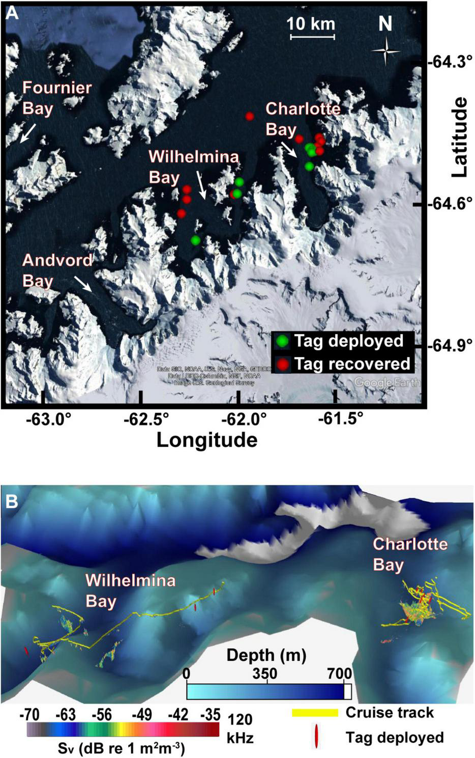
Study area. (A) Tag deployment and recovery locations in the two fjords along the West Antarctic Peninsula. (B) Oblique view of study area with survey track, tag deployment locations, and acoustically detected patches. Data plotted in Echoview v11 with 8× vertical exaggeration. Bathymetric data at 1 arcmin resolution (Globe Task Team et al., 1999). Resolution of bathymetric data means some acoustic data in this view is not visible.
Materials and Methods
Data Collection
The West Antarctic Peninsular fjords known as Charlotte and Wilhelmina Bays were explored from 12–16 March 2020 on board the RV Australis, a 23 m, steel-hulled, single-masted motor sailor with a relatively low environmental footprint. As a small, agile, and relatively quiet vessel, it can approach whales slowly without initiating a change in behavior (Danis et al., 2019). In both bays, whales were observed from the main vessel and general abundance estimates were made by two observers. We launched a zodiac tender from the ship to approach humpback whales for tagging, and a 6 m pole was used to deploy suction cup attached video and 3D accelerometer tags manufactured by Customized Animal Tracking Solutions (CATS) (Cade et al., 2016; Goldbogen et al., 2017a). All tags (except one, #62) were equipped with corrodible devices that released tension on tubes connected to the suction cups, flooding the tubes and releasing them from the animals within 24 h. Tag 62 was equipped only with a 1 Hz pressure sensor (no inertial sensors). All work was conducted under National Marine Fisheries Services and Antarctic Conservation Act permits, as well as approved institutional animal care protocols.
Whales were most approachable when “logging” at the surface (Schuler et al., 2019; Iwata et al., 2021) or when they were slowly surfacing while recovering from dives, and were least approachable when actively engaged in group bubble-net feeding. Tag accelerometers for all deployments were sampled at 400 Hz, magnetometers and gyroscopes at 50 Hz, and pressure, light, temperature and GPS at 10 Hz. All data were decimated to 10 Hz, tag orientation on the animal was corrected for, and animal orientation was calculated using custom-written scripts in Matlab 2014a (following Cade et al., 2021a). Animal speed for all deployments was determined using the amplitude of tag vibrations (Cade et al., 2018), and animal positions for the duration of each deployment were estimated from interpolating pseudotracks of the animal between known fast-acquisition GPS positions collected by the tags when the whales were at the surface and distributing accumulated error along the track (Wilson et al., 2007). Snowy conditions on all days precluded the estimation of tagged animal length from overhead imagery.
The prey field was sampled using pole-mounted, split-beam hydroacoustic echosounders sampling at 38 and 120 kHz with 12° and 7° beam widths, respectively. Simrad Ek80 wideband transceivers (WBT) were stored in a water-proof case with a 12 V battery that powered the whole system on an independent power source (Figure 2A). Low-frequency echosounders (e.g., 38 kHz and below) can record echoes returned from 1,000 m or more, even on noisy ocean-going ships. Higher-frequency pings, however, with correspondingly shorter wavelengths, are more subject to scatter and absorption (Simmonds and MacLennan, 2008) and generally operate at lower power, implying that under typical survey conditions the functional range of 120 kHz echosounders is <250 m (e.g., Watkins and Brierley, 1996; Bernard and Steinberg, 2013). For our study, the combination of operation in protected fjords with calm water conditions (Beaufort 0), an electrically isolated system and a quiet survey vessel allowed for the collection of clean acoustic data at both sampling frequencies down to at least 400 m when surveying at speeds up to 6 kts (Figure 2B).
FIGURE 2
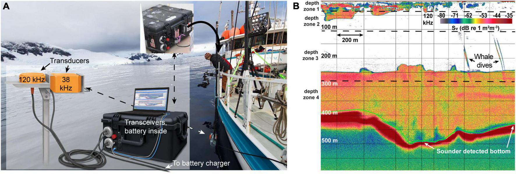
The mobile setup for the ek80 system, in combination with calm waters in the fjords, allows clean data collection. (A) The self-contained mobile system allows for sensitive transceivers to be deployed in open air boats with an independent power-supply (a 12 V deep-cycle marine battery). (B) Unprocessed 120 kHz ek80 data. This system allowed for clean data collection below 500 m depth at 120 kHz. Time-varied gain corrected background noise at 500 m was ∼-70 dB, implying a signal to noise ratio of >20 dB even at those depths. Photo credit: Ryan Houston, illustration by Alex Boersma.
Overlapping projects on the shared-use vessel precluded dedicated grid-survey patterns. Instead, prey data were collected intermittently in the vicinity of foraging and tagged whales as time permitted (Table 1) at 1 s ping intervals with pulse lengths of 1,024 μs. Due to a COVID-19-shortened expedition, an in situ calibration of the system was not performed for this season. Instead, calibration data (using a 38.1 mm tungsten carbide sphere, following Demer et al., 2015) of the same system in the same environment from the year prior was applied to all collected data. Because there may be drift in the system over time, biomass is reported herein for comparison purposes within this study and should not be used to predict actual biomass encountered by foraging whales without accounting for potential error from drifting sensitivity.
TABLE 1
| Hydroacoustic data | |||||||||||
| Date | Bay | Distance sampled | Start time (local) | End time (local) | Gulp-sized cells with krill | Dive-sized cells with krill | Empty water columns (dive-width) | Zone 1 (0–35 m) | Zone 2 (35–105 m) | Zone 3 (105–280 m) | Zone 4 (>280 m) |
|
|
|||||||||||
| DD/MM/YYYY | – | km | HH:MM | HH:MM | # | # | # | # of dive-sized cells with ≥30 gulps above 20 g/m3 | |||
|
|
|||||||||||
| 13/March/2020 | Charlotte | 37.6 | 9:30 | 18:10 | 259,521 | 1,313 | 36 | 82 | 14 | 364 | 608 |
| 14/March/2020 | Charlotte | 29.2 | 13:58 | 19:11 | 198,932 | 993 | 25 | 33 | 9 | 402 | 414 |
| 15/March/2020 | Wilhelmina | 39.4 | 8:31 | 18:26 | 142,946 | 958 | 30 | 116 | 47 | 361 | 182 |
Summary of hydroacoustic data collected.
Foraging Behavior
Lunge feeding events—the rapid engulfment of a mouthful of prey-laden water followed by subsequent filtration—were identified from the tag record (Figures 3A,B) via the identification of stereotyped maneuvers, typified by acceleration followed by rapid deceleration (Cade et al., 2016; Kahane-Rapport et al., 2020) as the whale is slowed from the engulfed water mass (Potvin et al., 2020). Tag ID mn200313-62, which only had a pressure sensor, was treated separately and lunge counts were estimated from the shape of the dive profile in combination with the vertical speed of the animal (similar to the method of Croll et al., 2001). Rorqual whale feeding behavior is a constant optimization problem balancing resource acquisition at depth with oxygen acquisition at the surface (Hazen et al., 2015). Stereotypical behavior consists of diving from the surface, performing from 1 to 10 or more discrete lunges, then surfacing for one to a dozen or more breaths and then diving to forage again.
FIGURE 3
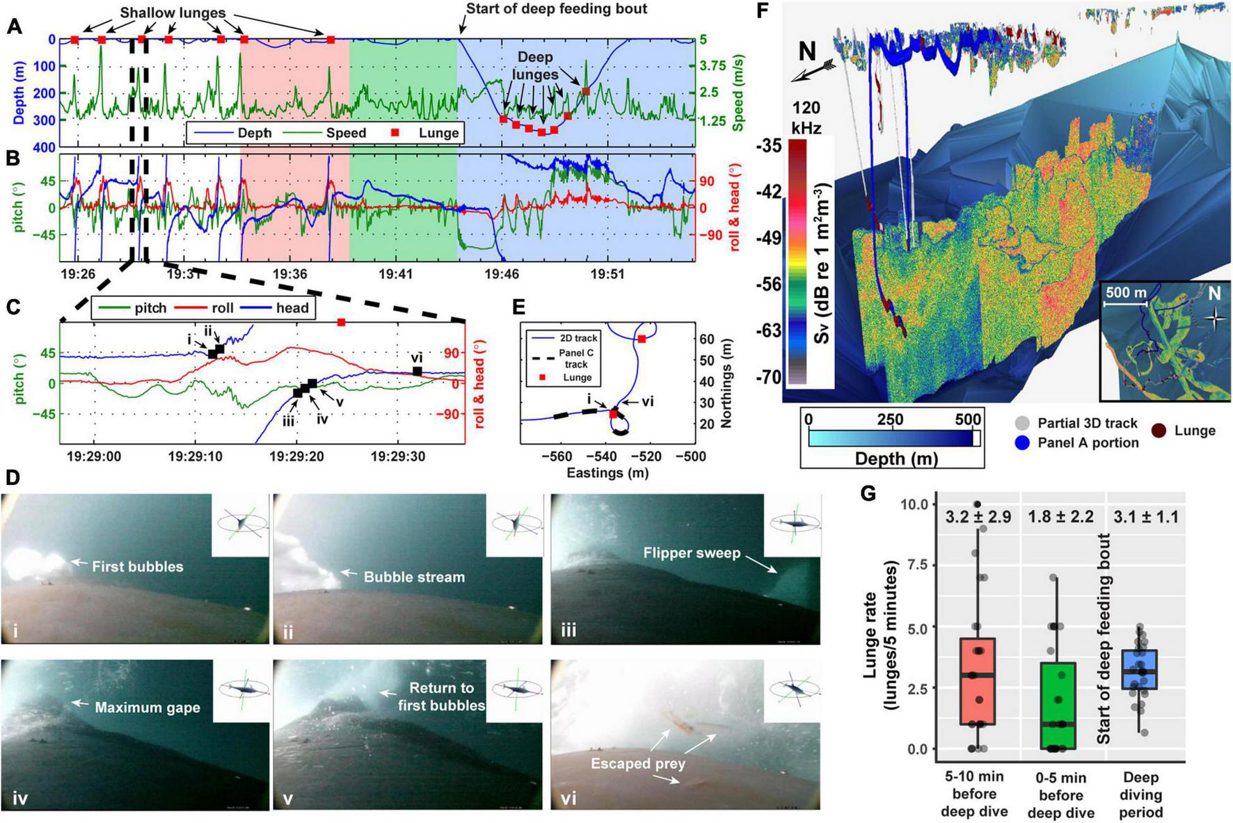
Transition from shallow to deep feeding. (A) Time series of depth and speed with locations of lunges marked. Background colors match the time periods of summary data in panel (G). (B) Time series of pitch, roll, and heading. All surface feeding events displayed are bubble-nets with 360° circles preceding the lunge. (C) Zoomed in version of pitch, roll and heading traces for a single bubble-net feeding event. (D) Video images from the tag corresponding to the time points marked in panel (C). (E) 2D track of two bubble nets, including the subsection plotted in panel (C). (F) 3D track spatially located with mapped prey data showing the transition from surface to deep feeding. Inset is overhead view for context (note that bathymetry color is not to scale in the inset). (G) Average number of lunges across all deployments preceding the onset of deep foraging, and the feeding rate during the first deep feeding events (feeding rate from the start of a dive until the start of the next dive). Box plots are median and inter-quartile range, numbers are lunges per 5 min (mean ± SD).
A series of foraging dives without a prolonged break between them is referred to as a foraging bout. For the duration of a foraging bout, prey is thought to be accessible at levels above the minimum thresholds required to recover spent energy (Friedlaender et al., 2009a,2013; Doniol-Valcroze et al., 2011; Goldbogen et al., 2011). The distribution of intervals between foraging dives (dives with at least one lunge) has been shown to be approximately normal in humpback and blue whales, but with a right-skewed tail (Cade et al., 2021b), suggesting a quantitative divider between surface intervals that can be considered part of the same foraging bout and those that are outliers and suggest association with some other behavior (e.g., searching or resting). To reduce the influence of other behaviors on what is classified as foraging effort (sensu Suter and Houston, 2020), we use 5.5 min, the threshold surface interval identified as the mean surface interval plus three standard deviations of the >9,000 foraging dives from 42 humpback whales analyzed by Cade et al. (2021b, Supplementary Figure 4), as the dividing line between foraging bouts. We then quantified the feeding rate (in lunges/h) of each individual tagged animal as the feeding rate within each foraging bout.
Foraging effort (foraging bout length and feeding rates) was quantified within four depth bins: 0–35 m, 35–105 m, 105–280 m and >280 m. The bins were chosen in increments of multiples of 35 m to match the spatial scale of prey analysis (see below) and the boundaries were chosen to best represent natural breaks in mean daytime prey density. Dive behavior was also classified according to diurnal period (day/night/twilight) as defined by angular sun position using the MATLAB package ‘‘Sunrise Sunset.1“ Twilight was defined as the period when solar elevation was <6° degrees below the horizon and was determined in order to exclude those time periods from daylight and nighttime hours but is excluded as an independent analytical period due to low sample size. Inter lunge interval (ILI) and the number of lunges per dive were also calculated in each depth bin as indicators of the spatial distribution of prey where a whale was diving.
Potential bubble-net feeding behavior, where whales blow a bubble ring near the surface before lunging through the middle of the ring (Jurasz and Jurasz, 1979; Wiley et al., 2011), was identified in tags with accelerometer data as shallow lunges (<20 m, ∼2 body lengths) that included a smooth horizontal turn (i.e., with a consistent angular velocity, Figures 3C,E) of at least 180° before the lunge. This classification was supported by direct observation of bubble production during lunging when cameras were active (e.g., Figure 3D and Supplementary Video 1); that is, in every instance where these maneuvers were observed on video, there were bubbles produced by the tagged whale. The bubble-net classification included both “typical” nets with at least one full 360° rotation as well as shorter maneuvers. Bubbles were also occasionally blown for surface lunges that did not include this maneuver. These streams were shorter and could be better classified as bubble bursts than the streams of bubbles more typically associated with bubble nets. Bubble net and surface feeding ILI were calculated to compare how the extra maneuvering of bubble net feeding affected feeding rates. Bubble-net and surface feeding ILI, a parameter usually calculated for the time between lunges on an individual dive, were calculated for consecutive lunges of the same type that were within 5.5 min, and surface feeding for this comparison was defined as lunges that occurred within the top 20 m of the water column (∼2 body lengths).
For all reported values, animal means were additionally averaged across animals, and standard deviations (SD) were pooled to get reported SDs. When reporting the feeding rate in each depth zone, each dive was assigned to a zone based on the deepest lunge depth of that dive.
Prey Analysis
Analysis of acoustic data was conducted at the “whale scale” (Cade et al., 2021b). This technique reports the distribution of analytical cells the size of a whale’s engulfment capacity, or gulp (hereafter: “gulp-sized cells”), within analytical cells the size that an average whale travels through on a dive (“dive-sized cells”). Specifically, we calculated the mean volume back scattering (MVBS) of the acoustic data (as Sv in dB re 1 m2/m3) within cells the size of the two-dimensional projection of an average humpback whale gulp (6 m long by 2.25 m high), and the distribution of this set of Sv data (mean ± SD) within cells the size that an average humpback whale explores from its first lunge to its last lunge (35 m high by 125 m long, calculated from tag data in Cade et al., 2021b). Acoustic energy in gulp-sized cells has been found to be normally distributed within dive-sized cells (i.e., biomass is lognormally distributed), so results are reported in Sv space as mean ± SD and, when converted to biomass, as geometric mean ⋅: geometric SD (where ⋅: is read “multiplied or divided by”).
To limit analysis to patches in which humpback whales were likely feeding, analysis was limited to dive-sized cells which contained at least 30 gulp-sized cells of at least 20 g/m3 of krill (Table 1). We believe this to be a conservative value since estimates of the minimum krill required for a species with similar energetic efficiencies (a blue whale) to recoup the cost of a lunge range from 20 g/m3 (Potvin et al., 2021) to 50 g/m3 (Goldbogen et al., 2011). We also calculated the distribution of biomass at the “informed whale scale” (details in Cade et al., 2021b), which reports the distribution of only the top half of gulp-sized cells in each dive-sized cell in allowance of probable discriminate foraging in denser parts of a patch (i.e., assuming that whales do not forage randomly within a patch).
Euphausia superba acoustic target strength (TS), used to enumerate abundance from Sv data, can be estimated from a krill’s body length (e.g., Jarvis et al., 2010). The TS of krill is strongly dependent on the size and mean orientation of individual animals, and the change in TS with size is more pronounced at lower frequencies (Wiebe et al., 1990; Stanton et al., 1998; Conti and Demer, 2006; Lawson et al., 2008). This phenomenon leads to larger differences between the measured return echoes from dual frequency systems when krill are smaller (Figure 4F).
FIGURE 4
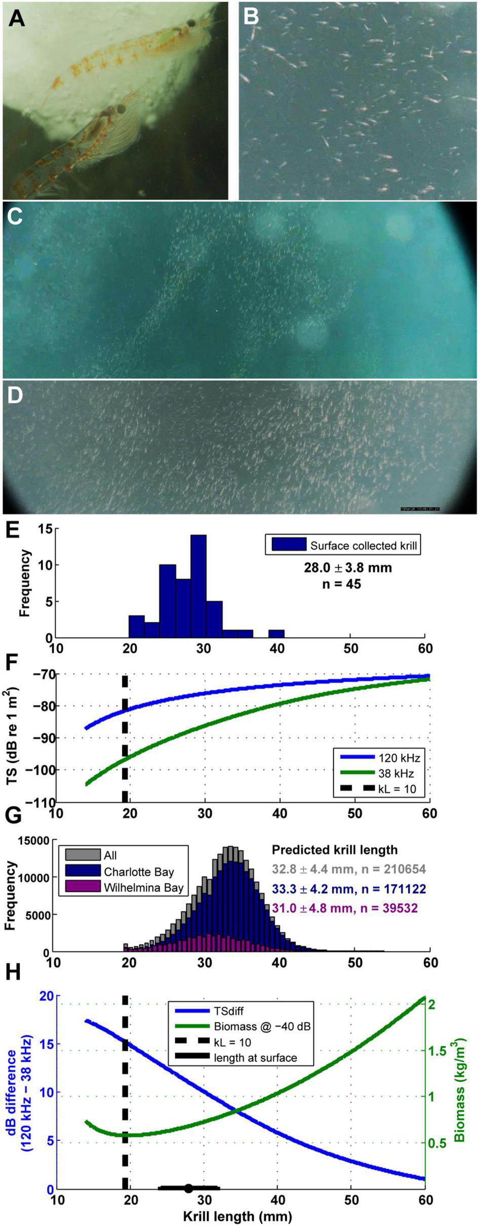
Euphausia superba behavior and size. (A) Live krill collected in Wilhelmina Bay, photo credit: Natural History New Zealand. (B–D) Surface krill filmed after the camera tag deployed on mn200315–58 detached from the animal (see also Supplementary Video 2). (E) Length frequency histogram of krill collected from the surface in Wilhelmina Bay (summary data are mean ± SD). (F) The difference in TS between 120 and 38 kHz echograms changes with krill length (calculated from the updated SDWBA model in Calise and Skaret, 2011). When kL (wave number times length) is less than 10, TS changes rapidly with length, implying that in practice measurements are unreliable. Dashed line is when kL = 10 for krill ensonified with a 120 kHz ping. (G) The predicted krill length of each measured gulp-sized cell in both bays under study. (H) For a given measured echo return (-40 dB shown as an example), the calculated biomass density is highly dependent on assumptions about krill length in a particular parcel of water. Dashed line is when kL = 10 for krill ensonified with a 120 kHz ping.
Typically, prey patches are identified as likely containing krill using the difference in measured returns between 38 and 120 kHz echosounders (e.g., Jarvis et al., 2010; Owen et al., 2017) and then enumerated using the 120 kHz data at an assumed TS value. The distribution of TS of krill in the water column is typically estimated from a distribution of lengths of krill collected via net tows within the survey region. However, the spatial resolution of trawling a net with a 4 m2 opening is much lower than the spatial resolution of acoustic prey mapping which can sample the entire water column for long continuous periods (Munger et al., 2009); as a result, typically a single distribution of krill sizes and TS are applied equally to all echosounder data to estimate all biomass in a survey region. For purposes of estimating total surveyed biomass, this is likely appropriate (e.g., Jarvis et al., 2010; Bernard et al., 2017). However, krill and other pelagic organisms often show both depth-stratified size segregation (Ichii et al., 2020) as well as size segregation within larger patches (Benoit-Bird et al., 2017), implying that large scale averaging and applications of single TS values may miss the underlying variability that characterizes patchy environments. Thus, to examine how predator-available prey biomass varies within a region, it would be useful to know how the size of krill varies within the survey region to better calculate TS (and thus better estimate abundance and biomass).
Accordingly, we estimated the TS of krill in our study in each gulp-sized and dive-sized analytical cell by calculating the 120–38 kHz dB difference, and back-calculating the assumed krill length and TS that would have generated the observed difference in each cell (using similar techniques as Lawson et al., 2008). The dB difference vs. krill length curves in Figures 4F,H were calculated using the updated SDWBApackage2010 from Calise and Skaret (2011), based on the SDWBA model from Conti and Demer (2006). The number of krill in each cell and the estimated biomass in each cell were then estimated following the procedures in Jarvis et al. (2010). We compared the inferred length to the length distribution of krill collected by hand by a diver at 1–2 m depth during the daylight in Wilhelmina Bay (Figures 4E,G).
Influence of Prey on Predator Foraging
The major difference between foraging behavior in the two bays appeared to be the frequency of deep (zone 4) foraging in Charlotte Bay during daylight hours (discussed below), so we ruled out biomass as a likely explanatory factor given its decreasing relationship with depth (see results). To test the influence of estimated krill length, patch thickness, and the number of patches in each zone on daylight foraging behavior in zone 4 vs. zone 3, foraging rate and prey data by zone were first summarized at two scales: (a) in 1-h bins (n = 281 h bins) and (b) associated with each dive individually (n = 109 individual dives with associated prey patches). For 1-h bins, the feeding rate in each zone in each hour was computed, and prey variables (mean estimated krill length, mean patch thickness, number of cells that meet the threshold for inclusion) were computed for all prey data collected within 5 km and 24 h of the convex polygon surrounding the whale’s estimated positions during each daylight hour, and the difference between zone 4 and zone 3 were compared. For the dive-by-dive summary, the same patch variables (mean estimated krill length, mean patch thickness, number of patches) measured within 250 m of each dive were summarized for each dive, and the interactions between the variables in the zone 3 and zone 4 depth bins were used as fixed effects. Generalized linear mixed effects (GLME) models were constructed in Matlab 2019a for both spatial scales to test the influence of the fixed effects on the response variables “proportion of dives in zone 4” (for the hourly summary) and “is the dive in zone 4?” for the dive-by-dive summary. Individual ID and time were used as random effects and were included in the null models. Variable influences on the models were compared in two ways: using a goodness-of-fit parameter that compares the R2 of the full model to the R2 of the model without the variable of interest (Cohen’s f2 as in Selya et al., 2012), and also using Akaike information criteria (AIC) in a forward model selection procedure.
Results
Predator Surface Observations
In Charlotte Bay, on March 12th and 13th, humpback whales were more densely concentrated in the eastern half of the bay. Whales were visually observed traveling singly, in pairs and, for short periods <15 min, in groups up to eight animals that would surface simultaneously with mouths agape after bubble rings ∼6–15 m in diameter were observed at the surface. Generally, individuals and pairs were spaced 100–500 m apart and spread throughout the eastern half of the bay in open, ice-free water. More than 100 individual whales were estimated to have been directly observed over the 2.5 days we spent in Charlotte Bay, and the actual population in the bay was estimated by observers to be more than 200 animals. On March 14th, we used VHF telemetry to relocate two tagged whales to the embayment on the east side of the fjord where an estimated 50–80 whales were distributed singly and in pairs (Figure 1). No bubble feeding was noted from surface observations or from tag data on this day. In all, six tags were deployed and recovered in Charlotte Bay (Table 2).
TABLE 2
| Foraging data by individual | ||||||||||
| Individual | Deployment duration | Time feeding | Daylight deployment duration | Night deployment duration | Daylight % spent feeding | Night % spent feeding | Daylight feeding rate* | Night feeding rate* | # foraging bouts | Mean bout length |
|
|
||||||||||
| spYYMMDD-tag# | h | h | h | h | % | % | Lunges/h | Lunges/h | Min | |
|
|
||||||||||
| Panel A: Charlotte Bay (12–14/March/2020) | ||||||||||
| mn200312-58 | 3.8 | 1.5 | 3.8 | – | 39% | – | 27.2 | – | 1 | 90.3 |
| mn200312-71 | 4.9 | 4.8 | 3.1 | 1.0 | 98% | 100% | 26.5 | 41.1 | 1 | 288.7 |
| mn200313-59 | 25.3 | 16.3 | 14.3 | 9.4 | 44% | 91% | 30.8 | 46.5 | 13 | 75.2 ± 34.0 |
| mn200313-60 | 13.6 | 9.0 | 8.0 | 4.7 | 44% | 100% | 38.3 | 53.9 | 7 | 78.0 ± 49.0 |
| mn200313-62 | 65.0 | 44.7 | 31.5 | 28.6 | 38% | 97% | 31.7 | 60.3 | 27 | 99.3 ± 45.6 |
| mn200313-70 | 18.3 | 15.7 | 7.2 | 9.4 | 88% | 83% | 35.6 | 38.6 | 16 | 59.0 ± 18.1 |
| Pooled summary | 58 ± 11% | 94 ± 3% | 31.7 ± 1.9 | 48.1 ± 4.0 | 115.1 ± 71.6 | |||||
| Panel B: Wilhelmina Bay (15–16/March/2020) | ||||||||||
| mn200315-54 | 18.3 | 10.0 | 7.0 | 9.6 | 9% | 91% | 19.6 | 34.4 | 10 | 59.8 ± 27.1 |
| mn200315-58 | 5.2 | 0.0 | 5.2 | – | 0% | – | – | – | – | – |
| mn200315-70 | 12.9 | 11.0 | 4.6 | 7.5 | 59% | 100% | 30.6 | 67.1 | 8 | 82.3 ± 66.2 |
| mn200315-71 | 0.3 | – | – | – | – | – | – | – | – | – |
| Pooled summary | 22 ± 18% | 95 ± 4% | 25.1 ± 5.5 | 50.8 ± 16.4 | 71.1 ± 98.7 | |||||
Deployment and foraging information for each tagged whale.
*Feeding rate within a foraging bout. Summaries are mean ± SD. Note that deployment mn200313-62 was only equipped with a pressure sensor (see text for details).
In contrast, the first whales observed upon entering Wilhelmina Bay on March 15th were at the northernmost tag deployment location in Wilhelmina (tag ID mn200315-58, Figure 1). Five whales were observed at this location. An additional 20–30 whales were observed near the southernmost deployment location (mn200315-70), and 10–20 whales were observed the following day in the same location. In contrast to Charlotte Bay, all daylight feeding behavior in Wilhelmina Bay was observed within accumulated brash ice or forming sea ice, or within 100 m of an ice edge (Figure 5). Overall abundance of humpback whales in Wilhelmina Bay was estimated to be ∼10–20% of the abundance in Charlotte Bay. Four tags were deployed on humpback whales in Wilhelmina, three of which stayed attached long enough to be included in our dataset (minimum 3 h) (Table 2). Five minke whales were additionally observed among the ice of Wilhelmina Bay, but none were observed in Charlotte Bay.
FIGURE 5
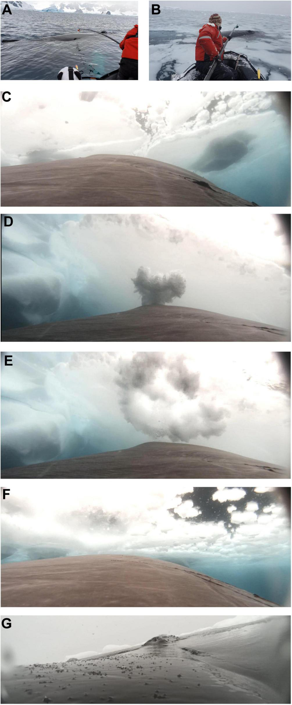
Environmental conditions in both bays. (A) In Charlotte Bay, all tags were deployed in ice free water and whales were not observed in icy conditions. (B) In Wilhelmina Bay, the two tags deployed on whales that subsequently foraged were in an icy inlet (Figure 1). (C–G) Still images from mn200315-58 in Wilhelmina Bay, clearing ice via bubble blasts to surface in open water (Supplementary Video 2). Stills D&E were from an earlier event than the other stills, but were included as representative of the process since they were clear images. Photo credits (A,B): Ryan Houston.
Predator Foraging Behavior
In Charlotte Bay, 58 ± 27% (mean ± SD) of overall tag on time during the day was identified as part of a feeding bout, while 95 ± 7% of tag on time at night was part of a feeding bout. In Wilhelmina Bay, 22 ± 32% of daylight hours were spent in feeding bouts, while 95 ± 6% of nighttime hours were spent in feeding bouts (Figure 6E). There was no difference between the percentage of time spent feeding in shallow waters (<35 m) during any temporal period in Charlotte Bay or during the day in Wilhelmina Bay (range: 10–14%), but the two tagged whales in Wilhelmina Bay that fed during the tag deployment spent <1% of their time feeding in shallow water at night (a total of 9 lunges). In Wilhelmina Bay, most daytime feeding was between 0 and 105 m (81% of time spent feeding), while in Charlotte Bay most daytime feeding (74% of the total) was >280 m. At night, whales from both Charlotte (59%) and Wilhelmina (54%) spent most of their time feeding between 105 and 280 m (Figure 6E).
FIGURE 6
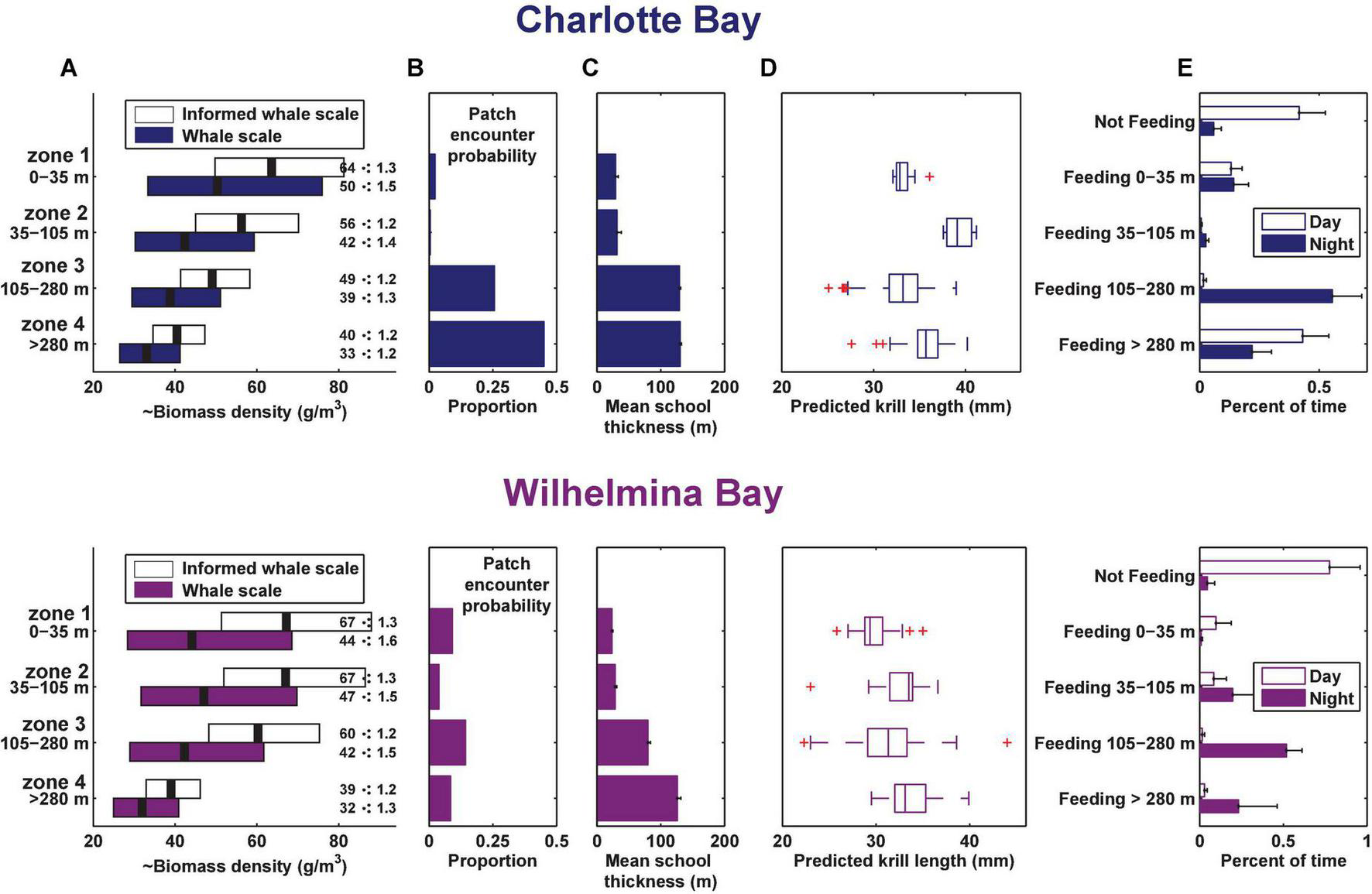
Summary of prey data and foraging behavior by depth zone in each bay. (A) Geometric mean and geometric standard deviation of biomass by depth zone (measured at the whale scale, where ⋅: means multiply or divide). (B) Proportion of columns of dive-sized analytical cells that contained a cell in the indicated zone with krill data above the threshold for inclusion (see section “Materials and Methods”), standardized for the height of the column. (C) Mean school thickness of patches in dive-sized cells in each depth zone. (D) Estimated krill length from 120 to 38 kHz dB differencing in each gulp-sized cell in the depth zone. Boxes are min, first quartile, median, third quartile, max data points, excluding outliers. (E) Mean percent of time spent by the tagged whales in each behavior. Error bars in panels (B,C,E) are standard error.
Bubble net feeding was observed in the tag records of whales in both bays. A total of 163 bubble nets were identified in the tag records of Charlotte Bay animals (22% of daytime lunges) and 19 in Wilhelmina Bay. The thirteen bubble nets from mn200315-54 (in Wilhelmina Bay) were identified during twilight (62% of twilight lunges), and the remainder were during daylight hours (7% of daylight lunges). Nets were all created clockwise in direction and averaged 352 ± 92° of rotation preceding the lunge. We made approximately twenty observations of bubble nets from the surface over the 5 day field period that were followed by several whales surface lunging and camera data confirmed close-proximity, nearly simultaneous lunges by conspecifics (Supplementary Video 1). In all except one case, sequences of bubble-net feeding within a foraging bout were not interrupted by typical (i.e., non-bubble net) lunge feeding. The inter-lunge interval (ILI) of these nets averaged 107 ± 42 s, while the ILI for surface feeding lunges when not bubble net feeding was ∼40% smaller (63 ± 34 s, n = 7, two-sided t-test p = 0.07). Three out of four animals with both types of lunges demonstrated significantly lower (p < 0.01) surface feeding ILI.
The feeding rate within foraging bouts was consistent across depth levels during the day, with no significant differences across depth zones or between bays. At night in both bays, foraging rate decreased with depth (Figure 7). Across all whales, 16 of 58 bouts of deep feeding (>105 m) were preceded by a bout of shallow feeding. During the time period 10–5 min before the onset of the first deep foraging dive, whales averaged 3.2 ± 2.9 shallow lunges (Figure 3G). This was significantly more (paired t-test, p < 0.01) than the following 5 min, in which whales averaged 1.8 ± 2.2 lunges, but approximately the same as the feeding rate (standardized to 5 min bins) of the first deep feeding dive (3.1 ± 1.1 lunges, p > 0.9).
FIGURE 7
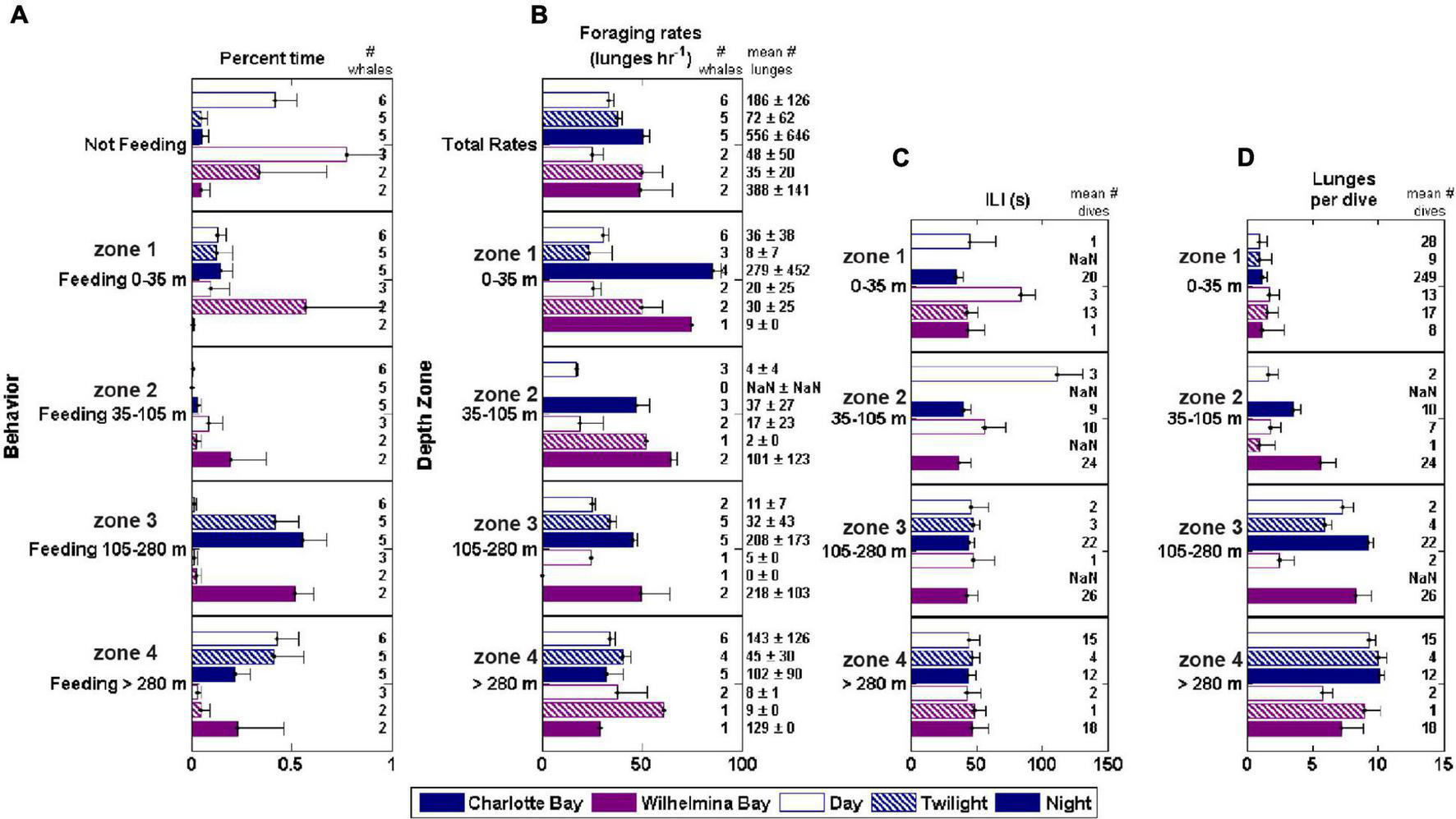
Foraging behavior by depth zone, bay and diel period. ILI, inter-lunge-interval. Foraging rate is lunges/h while actively foraging (lunge rate within a defined feeding bout). (A) Percent time feeding in each zone. (B) Foraging rate in each zone. (C) Mean ILI in each zone (D) Mean lunges/dive in each zone.
Prey
In both bays, daytime prey was generally distributed in small patches near the surface and large swarms at depth (Figures 3F, 6C, 8C): mean zone 1 patch thickness was 29 ± 13 m in Charlotte and 23 ± 9 m in Wilhelmina, while mean zone 4 patches were 130 ± 45 and 126 ± 47 m thick, respectively. Surface swarms could be diffuse and loosely organized, or could have separate tendrils containing individuals with similar alignment (Figures 4B,C and Supplementary Video 2). Charlotte Bay was characterized by an almost complete absence of krill between 80 and 150 m (generally aligning with depth zone 2), while the absence band in Wilhelmina Bay was somewhat smaller (Figures 8A,B). In both bays, the depth of maximum dB difference (implying smallest krill length) was at ∼200 m, while the smallest dB differences (largest krill) were at ∼400 m.
FIGURE 8
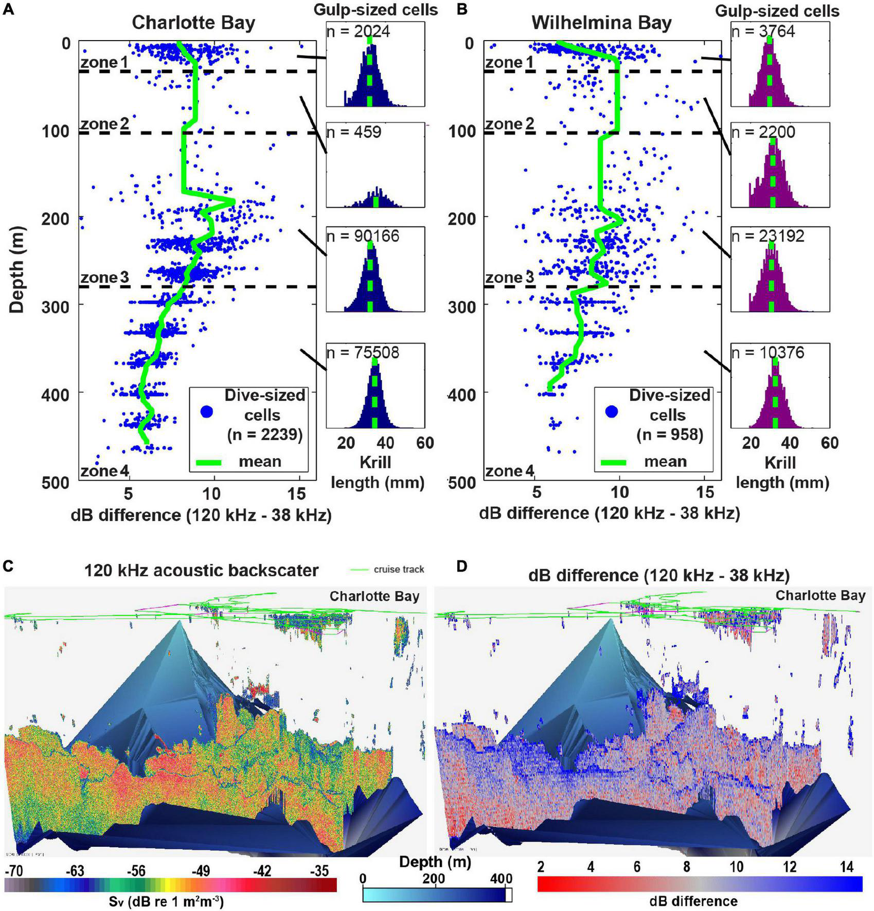
Mean krill size changes with depth. (A) Charlotte Bay dB differencing in dive-sized cells (left) and the distribution of krill lengths predicted from the dB differences of gulp-sized cells (right) in each depth zone. Note that the relationship of krill size to depth was similar for gulp-sized cells and dive-sized cells, but dive-sized cells are presented here for clarity of the graph. (B) Same as panel (A) but for Wilhelmina Bay. Note that the mean in zone 1 (29.6 ± 4.4 mm) is similar to the measured length of krill collected at the surface (28.0 ± 3.8 mm). (C) Acoustic backscatter (a proxy for biomass) in the surveyed region of Charlotte Bay. Bottom data interpolated from the sounder-detected bottom. (D) 120 –38 kHz dB differencing (of each gulp-sized cell) in Charlotte Bay. Red values (small dB difference) imply larger krill.
Prey biomass density within patches was not significantly different between bays (Figure 6A), except in depth zone 3, where the geometric mean of prey density at the informed whale scale was 22% higher in Wilhelmina Bay, and 8% higher at the whale scale (p < 0.001 in both cases). Zone 3 biomass was significantly higher (p < 0.001) than zone 4 biomass in both bays as well (Figure 6A). Dive-sized cells with sufficient krill to be included in analysis were the most common in zone 3 in Wilhelmina Bay and zone 4 in Charlotte Bay (Figure 6B), and patches were substantially thicker below 105 m in both bays (Figure 6C). Excluding zone 2 (due to limited sample size, see Table 1 and Figure 8), in both bays zone 4 had the largest predicted krill sizes (p < 0.001), and Charlotte Bay had larger krill than Wilhelmina Bay across zones (Figure 6D).
GLME results were inconclusive at both summary scales. For both scales, the null model (hourly scale: AIC = 122, dive-by-dive scale: AIC = 531) and the model containing just the number of patches variable (hourly scale: AIC = 120, dive-by-dive scale: AIC = 532) resulted in the lowest AIC scores. Additionally, for the data summarized in hourly bins, high temporal auto-correlation was noted; when the null model included time as a random effect, R2 = 0.87, if time were excluded from the null model, R2 = 0.49. At both scales, krill length demonstrated the highest effect sizes of the three tested variables (hourly scale Cohen’s f2: krill length = 0.07, patch thickness = 0.02, number of patches = -0.02; dive-by-dive scale Cohen’s f2: krill length = 0.99, patch thickness = 0.12, number of patches = 0.00). Given the null model AIC, the high effect sizes of the length variables, the effects of temporal autocorrelation, and the low sample sizes overall, the modeling approach did not provide sufficiently strong evidence given the current sample size for a relationship between krill patch characteristics and whale foraging at depth.
Discussion
Both globally in the present day and historically within the West Antarctic Peninsula (prior to commercial whaling) there appear to be more baleen whale species coexisting than would be expected (Perrin, 1991), especially given that many baleen whales have nearly global ranges and all feed in a similar manner and can feed on similar prey. In this study we sought to uncover the axis of heterogeneity that differentiates two habitats, one (Charlotte Bay) supporting approximately an order of magnitude more predators during our observation period.
The unique foraging style of rorqual whales, engulfment filtration feeding, typically implies that the biomass of prey within a mouthful of water is the ecological unit comparable to the single prey item of pursuit hunters (e.g., a bear or killer whale hunting a fish). From this standpoint, a foraging whale should seek to maximize ingested biomass per gulp regardless of the size of each individual prey. Thus, it was surprising to find that during the day in both bays we observed that the geometric mean biomass of krill per mouthful was smaller in zone 4 (>280 m) at depths where most daytime foraging occurred than in shallower depths through which these whales transited (Figure 6). This would appear to imply that, all else being equal, humpback whales would get less energy feeding in the deep waters of zone 4 than the more accessible zone 3. Equally surprising, zone 3 biomass was significantly higher in Wilhelmina Bay than in Charlotte Bay, suggesting it would have been a better place for whales to aggregate.
Box 1. Particle size influence on encounter rate for continuous ram filtration feeders.
Ivlev (1960) discusses how, if mean biomass concentration is held constant, larger particles will lead to a higher mean encounter rate of biomass for a forager. To see this, imagine that a continuous ram filter feeder like a menhaden feeds in two environments, both with the same mean biomass density ρ g/m3. Environment A has particle mass m g/individual, leading to a concentration, q, of ρ/m individuals/m3 and an encounter rate for a straight-traveling forager of individuals/m, with a biomass encounter rate, R, of m. If environment B has the same biomass density, but particles are twice as big (2m), then qB = qA/2, and RB = 2mA ≈ 1.6RA, implying that for these foragers larger particles lead to higher resource availability, even if the overall biomass in the environment is the same.
In temperate waters, both humpback whales and blue whales have been shown to aggregate not just where prey is more dense, but also more evenly distributed, minimizing the time between lunges (Cade et al., 2021b). Yet we found that zone 4 does not demonstrate reduced spacing between gulps since gulp-sized parcels of water were evenly distributed in both deep zones (GSD 1.2-1.5, Figure 6A), and whales also spent about the same amount of time between lunges in both zones (Figure 7C). In any system, but particularly systems where patchy prey are targeted, it is critical to match the spatial and temporal measurement of prey to the spatial and temporal scales exploited by the predators, yet effectively describing the distribution of resources at appropriate scales remains a challenge in ecology (Levin, 1992; Benoit-Bird et al., 2013; Chave, 2013). We utilized a predator-scale spatial analysis of prey patches to overcome the descriptive challenges; however, due to limitations on field time and equipment, our ability to match the spatial location of prey data collected to the precise patches where whales were foraging was limited (e.g., only 109 out of 1,705 foraging dives had prey measured within 250 m of the dive). Thus, we did not have sufficient statistical power to look at the effect of prey on the foraging performance of individual dives, and future work with better spatial matching of foraging effort and prey metrics is warranted. However, the large number of whales in Charlotte Bay suggested that patterns we noted at broad scales, including decreased biomass at depth and increased mean krill length at depth, could provide an explanation for the observed predator behaviors.
If energetically equivalent prey is targeted, overall energetic efficiency is expected to diminish at increasing distances from a central place, in this case the sea surface for air breathing humpback whales (Schoener, 1979). Our GLME models could not differentiate between increasing prey availability with depth (patch thickness and number of patches) from increasing krill length with depth as explanatory variables (Figures 6D, 8). However, given the extensiveness of the prey patches—presumably making them easy to locate—the most parsimonious explanation for why we found humpback whales diving deeper for less overall food biomass per gulp likely relates to food quality. Active selection of prey based on size is common in both marine and terrestrial ecosystems: both bears (Quinn and Kinnison, 1999) and Eastern Pacific killer whales (Ford and Ellis, 2006) hunting salmon select larger individuals to increase their take per unit effort; juvenile Coho salmon select smaller prey since they are easier to catch (Parker, 1971); Risso’s dolphins (Visser et al., 2021) and kookaburras (Blomberg and Shine, 2000) appear to target smaller-size cohorts of their preferred prey species since their habitat makes them more available; and filter-feeding fish, such as menhaden, have been shown to target habitat with larger average prey size, “regardless of where in the transect the highest total biomass concentrations occurred” (Friedland et al., 1989). For continuous ram filtration feeders, particle-size matters since for a given biomass density in the water column, larger particles will lead to more biomass encountered per unit time (Box 1). Humpback whales, however, engulf thousands of krill with a single mouthful, so preferential selection of larger krill only makes sense if larger krill are in some way easier to catch or easier to assimilate for a given biomass. We can reject the former since larger krill are more mobile (have faster escape speeds, Kils, 1979, 1981) and we found that they were less accessible (deeper), suggesting that some aspect of their physical properties may make them more desirable prey.
The lipid content of Antarctic krill can vary by an order of magnitude even within a single sampling location, from <1% of wet weight to >10%, and the proportion of the energy storage lipid tricylglycerol also has large variability within krill lipid stores (Pond et al., 1995). Adult humpback whales typically gain ∼50% of their body weight during a 3–4 month foraging season (Lockyer, 1981) with an estimated rate of 0.9 tons of body mass added per foraging week (Ash, 1953), suggesting that the ability to selectively forage on lipid-rich prey may be an important enhancement as lipids in prey are likely easier to turn into fat reserves in the predator and can lead to improved reproductive success (Golet et al., 2000). Humpback whales feeding along the West Antarctic Peninsula show a declining feeding rate throughout the foraging season (Nichols, 2020), and by March 13, more than 130 days after the canonical start of the foraging season, most humpback whale size classes demonstrate an asymptotic or maximum body size index (Figure 3.4 in Bierlich, 2021), implying a slowing rate of weight gain and decreased need to forage. Given that whales spend about half their daylight hours not actively feeding (Figure 7A), and given that they have likely accumulated the bulk of the energy stores needed for their annual migration, it would appear to benefit these animals to mostly target krill that are digestively easy to assimilate.
Current acoustic techniques cannot differentiate the lipid content of krill, but prior research has observed depth-stratified size segregation of krill (Friedlaender et al., 2016b; Ichii et al., 2020), specifically observing large, gravid females (Clarke and Tyler, 2008) that are likely foraging on the benthos (Schmidt et al., 2011). If the scattering difference between 120 and 38 kHz frequencies we detected acoustically signify larger, more lipid-rich krill as we suggest, it would indicate a resolution to the paradox of why whales in Charlotte Bay feed deeper during the day than the depths of maximum biomass, and also offers an explanation for why more whales were aggregating in Charlotte than in Wilhelmina Bay, since Charlotte Bay not only has larger krill on average (Figure 4G), it also contained extensive, deep patches at depth that appeared to contain larger krill (Figure 6D).
In a prior study by Santora et al. (2010), fin whales were found near larger krill (>45 mm) while humpback whales were found in habitats with small/juvenile krill (<35 mm), similar to our size range (mean 32.8 ± 4.4 mm, Figure 4G). However, humpback whales in our study demonstrated two behavioral tactics that appeared to allow exploitation of the larger krill present within the overall habitat. Firstly, humpback whales forage in a three-dimensional environment, and the deep dives we recorded (maximum depth 459 m, 74% of foraging bout duration in Charlotte Bay were on dives > 280 m) were some of the deepest foraging dives recorded in the literature. Despite recording 29 individual dives greater than 400 m in our data set, we only found one other study with humpback whale dives deeper than 400 m (Derville et al., 2020) and the previous deepest dive reported in the Antarctic was 388 m (Friedlaender et al., 2013), suggesting Charlotte Bay whales are pushing their physiological limits to capture high quality food.
Secondly, krill at the surface were patchier than at depth (Figures 2B, 4C, 8C), though some patches contained large krill (Figure 8A). Bubble netting is a behavior unique to humpback whales, and though it has been observed in fish-feeding populations for many decades (Jurasz and Jurasz, 1979), it has only recently been reported in Southern Hemisphere krill feeding populations (Acevedo et al., 2011). Humpback whales use bubble netting to concentrate prey before lunging, allowing them to exploit patches that otherwise would not have sufficient prey to make foraging worthwhile (Figures 4A–D). By staying close to the surface, the transit time between the surface and prey is reduced, but because prey requires manipulation, it takes longer between bubble nets (mean bubble net ILI 107 ± 42 s, mean non-bubble net surface feeding ILI 63 ± 34 s, mean zone 4 ILI 46 ± 15 s). In this study, we noted that whales switched behavior between shallow and deep feeding when the surface foraging rate dropped (Figure 3G), and that similar overall foraging rates existed before the 5 min preceding deep feeding as during deep feeding, suggesting that when prey was no longer distributed as to be amenable to surface feeding, the deep, consistent prey layer in Charlotte Bay provided whales an opportunity to continue feeding.
More than 1.6 million baleen whales were taken from the Southern Ocean in the twentieth century (Rocha et al., 2014), and the impact of this massive biomass loss on nutrient cycling and krill populations generally have been the focus of recent studies (Croll et al., 2006; Pershing et al., 2010; Roman et al., 2014). In other ecosystems, the introduction of predators can have profound effects on the structure of prey size distributions (Lazzaro et al., 2009), and studies in other ecosystems have also suggested that rorqual whales may be capable of size-differentiated foraging strategies. For example, in the Northeast Pacific, krill found in blue whale feces are consistently found to be larger than the mean krill sizes collected via net-tows in the regions (Croll et al., 2005; Nickels et al., 2018). The effect that selection of larger krill sizes by an increasing rorqual whale population may have on krill population structure, however, has not been considered.
Although humpback whale populations are recovering and high pregnancy rates in the West Antarctic Peninsula suggest they are not currently resource limited (Pallin et al., 2018), as of 2004 blue whale populations were still less than 1% of historic abundances (Branch, 2007) and remain at such low densities that accurate population estimates are difficult (Paarman et al., 2021). Thus, two critical questions that could have cascading influence over this globally important ecosystem are good avenues for further research: (1) How the recovery of baleen whales will influence Southern Ocean krill population dynamics, and (2) whether horizontal and vertical size segregation provide an axis of heterogeneity that would support multiple niches for baleen whale species with different foraging needs.
It appears evident that the fjords along the West Antarctic Peninsula are key foraging grounds for behaviorally adaptable humpback whales throughout their feeding season, but which fjord provides the best foraging conditions and draws the most whales appears to vary both within and across seasons (Nowacek et al., 2011, this study, personal obs.). We found that Charlotte Bay specifically can support a large population of both predators and prey and is likely important habitat for this protected species. Future research should examine the forces that drive year-by-year changes in the region that may indicate the size and availability of krill in the region on a year-by-year basis. Such information could then be used to support adaptive fisheries management tools (e.g., Hinke et al., 2017) that could direct fisheries efforts to regions of appropriately high biomass that do not also demonstrate krill size and aggregation properties that are the preferred targets of protected marine species like the humpback whales studied here.
Publisher’s Note
All claims expressed in this article are solely those of the authors and do not necessarily represent those of their affiliated organizations, or those of the publisher, the editors and the reviewers. Any product that may be evaluated in this article, or claim that may be made by its manufacturer, is not guaranteed or endorsed by the publisher.
Statements
Data availability statement
The datasets presented in this study can be found in online repositories. The names of the repository/repositories and accession number(s) can be found below: https://purl.stanford.edu/mk884mg4167.
Ethics statement
The animal study was reviewed and approved by the University of California, Santa Cruz Institutional Animal Care and Use Committee.
Author contributions
DC, BW, and AF: conceptualization. DC, SK-R, and BW: investigation. DC and SK-R: formal analysis. JG and AF: funding acquisition and supervision. DC: methodology and writing—original draft. DC, SK-R, JG, and AF: writing—review and editing. All authors contributed to the article and approved the submitted version.
Funding
Funding for field work provided by Natural History New Zealand. Other funding for equipment and analysis provided by grants from the World Wildlife Fund, National Science Foundation (OPP-1643877), the Office of Naval Research (YIP grant #N000141612477 and DURIP grant #N000141612546), and Stanford University’s Terman Fellowship.
Acknowledgments
We gratefully thank the Natural History New Zealand for their financial support of this field effort, as well as Ryan Houston and Katie Lucas of the MSY Australis for field support.
Conflict of interest
BW was the captain of the field vessel and has a financial interest in the success of research projects. The remaining authors declare that the research was conducted in the absence of any commercial or financial relationships that could be construed as a potential conflict of interest.
Supplementary material
The Supplementary Material for this article can be found online at: https://www.frontiersin.org/articles/10.3389/fmars.2022.747788/full#supplementary-material
Supplementary Video 1Video from on-animal cameras with associated accelerometry data indicating bubble net feeding.
Supplementary Video 2Krill swarms at the surface filmed after the camera tag detached from mn200315-58. Also shown: video of bubbles being blown to clear the surface of ice (as in Figure 5).
References
1
Abrahms B. Hazen E. L. Aikens E. O. Savoca M. S. Goldbogen J. A. Bograd S. J. et al (2019). Memory and resource tracking drive blue whale migrations.Proc. Natl. Acad. Sci. U.S.A.1165582–5587. 10.1073/pnas.1819031116
2
Acevedo J. Plana J. Aguayo-Lobo A. Pastene L. A. (2011). Surface feeding behavior of humpback whales in the magellan strait.Rev. Biol. Mar. Oceanogr.46483–490. 10.4067/S0718-19572011000300018
3
Ash C. (1953). Weights of antarctic humpback whales.Norsk Hvalfangsttid42387–391.
4
Benoit-Bird K. J. Battaile B. C. Heppell S. A. Hoover B. Irons D. Jones N. et al (2013). Prey patch patterns predict habitat use by top marine predators with diverse foraging strategies.PLoS One8:e53348. 10.1371/journal.pone.0053348
5
Benoit-Bird K. J. Moline M. A. Southall B. L. (2017). Prey in oceanic sound scattering layers organize to get a little help from their friends.Limnol. Oceanogr.622788–2798. 10.1002/lno.10606
6
Bernard K. S. Steinberg D. K. (2013). Krill biomass and aggregation structure in relation to tidal cycle in a penguin foraging region off the Western Antarctic Peninsula.ICES J. Mar. Sci.70834–849. 10.1093/icesjms/fst088
7
Bernard K. S. Cimino M. Fraser W. Kohut J. Oliver M. J. Patterson-Fraser D. et al (2017). Factors that affect the nearshore aggregations of Antarctic krill in a biological hotspot.Deep Sea Res. Part I126139–147. 10.1016/j.dsr.2017.05.008
8
Bierlich K. C. (2021). Incorporating Photogrammetric Uncertainty in UAS-based Morphometric Measurements of Baleen Whales.Ph.D. thesis. Durham, NC: Duke University.
9
Blomberg S. P. Shine R. (2000). Size-based predation by kookaburras (Dacelo novaeguineae) on lizards (Eulamprus tympanum: Scincidae): what determines prey vulnerability?Behav. Ecol. Sociobiol.48484–489. 10.1007/s002650000260
10
Branch T. A. (2007). Abundance of Antarctic blue whales south of 60 S from three complete circumpolar sets of surveys.J. Cetacean Res. Manag.9253–262.
11
Burrows J. A. Johnston D. W. Straley J. M. Chenoweth E. M. Ware C. Curtice C. et al (2016). Prey density and depth affect the fine-scale foraging behavior of humpback whales Megaptera novaeangliae in Sitka Sound, Alaska, USA.Mar. Ecol. Prog. Ser.561245–260. 10.3354/meps11906
12
Cade D. E. Barr K. R. Calambokidis J. Friedlaender A. S. Goldbogen J. A. (2018). Determining forward speed from accelerometer jiggle in aquatic environments.J. Exp. Biol.221:jeb170449. 10.1242/jeb.170449
13
Cade D. E. Friedlaender A. S. Calambokidis J. Goldbogen J. A. (2016). Kinematic diversity in rorqual whale feeding mechanisms.Curr. Biol.262617–2624. 10.1016/j.cub.2016.07.037
14
Cade D. E. Seakamela S. M. Findlay K. P. Fukunaga J. Kahane-Rapport S. R. Warren J. D. et al (2021b). Predator-scale spatial analysis of intra-patch prey distribution reveals the energetic drivers of rorqual whale super group formation.Funct. Ecol.35894–908. 10.1111/1365-2435.13763
15
Cade D. E. Gough W. T. Czapanskiy M. F. Fahlbusch J. A. Kahane-Rapport S. R. Linsky J. M. J. et al (2021a). Tools for integrating inertial sensor data with video bio-loggers, including estimation of animal orientation, motion, and position.Anim. Biotelem.9:34. 10.1186/s40317-021-00256-w
16
Calise L. Skaret G. (2011). Sensitivity investigation of the SDWBA Antarctic krill target strength model to fatness, material contrasts and orientation.Ccamlr Sci.1897–122.
17
Chave J. (2013). The problem of pattern and scale in ecology: what have we learned in 20 years?Ecol. Lett.164–16. 10.1111/ele.12048
18
Clarke A. Tyler P. A. (2008). Adult Antarctic krill feeding at abyssal depths.Curr. Biol.18282–285. 10.1016/j.cub.2008.01.059
19
Conti S. G. Demer D. A. (2006). Improved parameterization of the SDWBA for estimating krill target strength.ICES J. Mar. Sci.63928–935. 10.1016/j.icesjms.2006.02.007
20
Croll D. A. Acevedo-Gutiérrez A. Tershy B. R. Urbán-RamıRez J. (2001). The diving behavior of blue and fin whales: is dive duration shorter than expected based on oxygen stores?Comp. Biochem. Physiol. Part A129797–809. 10.1016/S1095-6433(01)00348-8
21
Croll D. A. Kudela R. Tershy B. R. (2006). “Ecosystem impact of the decline of large whales in the North Pacific,” in Whales, Whaling and Ocean Ecosystems, ed.EstesJ. A. (Berkeley, CA: University of California Press), 202–214. 10.1525/california/9780520248847.003.0016
22
Croll D. A. Marinovic B. Benson S. Chavez F. P. Black N. Ternullo R. et al (2005). From wind to whales: trophic links in a coastal upwelling system.Mar. Ecol. Prog. Ser.289117–130. 10.3354/meps289117
23
Croxall J. Prince P. Reid K. (1997). Dietary segregation of krill-eating South Georgia seabirds.J. Zool.242531–556. 10.1111/j.1469-7998.1997.tb03854.x
24
Danis B. Christiansen H. Guillaumot C. Heindler F. Houston R. Jossart Q. et al (2019). Report of the Belgica 121 Expedition to the West Antarctic Peninsula. Available online at: https://zenodo.org/record/4551452(accessed February 19, 2021).
25
Demer D. Berger L. Bernasconi M. Bethke E. Boswell K. Chu D. et al (2015). Calibration of acoustic instruments.ICES Coop. Res. Rep.326:133. 10.1001/jamaophthalmol.2014.5265
26
Derville S. Torres L. G. Zerbini A. N. Oremus M. Garrigue C. (2020). Horizontal and vertical movements of humpback whales inform the use of critical pelagic habitats in the western South Pacific.Sci. Rep.101–13. 10.1038/s41598-020-61771-z
27
Doniol-Valcroze T. Lesage V. Giard J. Michaud R. (2011). Optimal foraging theory predicts diving and feeding strategies of the largest marine predator.Behav. Ecol.22880–888. 10.1093/beheco/arr038
28
Ducklow H. W. Baker K. Martinson D. G. Quetin L. B. Ross R. M. Smith R. C. et al (2007). Marine pelagic ecosystems: the west Antarctic Peninsula.Philos. Trans. R. Soc. B36267–94. 10.1098/rstb.2006.1955
29
Findlay K. P. Seakamela S. M. Meÿer M. A. Kirkman S. P. Barendse J. Cade D. E. et al (2017). Humpback whale “super-groups” – a novel low-latitude feeding behaviour of Southern Hemisphere humpback whales (Megaptera novaeangliae) in the Benguela Upwelling System.PLoS One12:e0172002. 10.1371/journal.pone.0172002
30
Ford J. K. Ellis G. M. (2006). Selective foraging by fish-eating killer whales Orcinus orca in British Columbia.Mar. Ecol. Prog. Ser.316185–199. 10.3354/meps316185
31
Ford R. G. Ainley D. G. Lescroël A. Lyver P. O. B. Toniolo V. Ballard G. (2015). Testing assumptions of central place foraging theory: a study of Adélie penguins Pygoscelis adeliae in the Ross Sea.J. Avian Biol.46193–205. 10.1111/jav.00491
32
Fraser W. R. Hofmann E. E. (2003). A predator’s perspective on causal links between climate change, physical forcing and ecosystem response.Mar. Ecol. Prog. Ser.2651–15. 10.3354/meps265001
33
Friedlaender A. S. Bowers M. T. Cade D. Hazen E. L. Stimpert A. K. Allen A. N. et al (2020). The advantages of diving deep: fin whales quadruple their energy intake when targeting deep krill patches.Funct. Ecol.34497–506. 10.1111/1365-2435.13471
34
Friedlaender A. S. Fraser W. R. Patterson D. Qian S. S. Halpin P. N. (2008). The effects of prey demography on humpback whale (Megaptera novaeangliae) abundance around Anvers Island, Antarctica.Polar Biol.311217–1224. 10.1007/s00300-008-0460-x
35
Friedlaender A. S. Goldbogen J. A. Hazen E. L. Calambokidis J. Southall B. L. (2014). Feeding performance by sympatric blue and fin whales exploiting a common prey resource.Mar. Mamm. Sci.31345–354. 10.1111/mms.12134
36
Friedlaender A. S. Hazen E. L. Goldbogen J. Stimpert A. Calambokidis J. Southall B. (2016a). Prey-mediated behavioral responses of feeding blue whales in controlled sound exposure experiments.Ecol. Appl.261075–1085. 10.1002/15-0783
37
Friedlaender A. S. Lawson G. L. Halpin P. N. (2009b). Evidence of resource partitioning between humpback and minke whales around the western Antarctic Peninsula.Mar. Mamm. Sci.25402–415. 10.1111/j.1748-7692.2008.00263.x
38
Friedlaender A. S. Hazen E. L. Nowacek D. P. Halpin P. N. Ware C. Weinrich M. T. et al (2009a). Diel changes in humpback whale Megaptera novaeangliae feeding behavior in response to sand lance Ammodytes spp. behavior and distribution.Mar. Ecol. Prog. Ser.39591–100. 10.3354/meps08003
39
Friedlaender A. S. Johnston D. W. Tyson R. B. Kaltenberg A. Goldbogen J. A. Stimpert A. K. et al (2016b). Multiple-stage decisions in a marine central-place forager.R. Soc. Open Sci.3:160043. 10.1098/rsos.160043
40
Friedlaender A. S. Joyce T. Johnston D. W. Read A. J. Nowacek D. P. Goldbogen J. A. et al (2021). Sympatry and resource partitioning between the largest krill consumers around the Antarctic Peninsula.Mar. Ecol. Prog. Ser.6691–16. 10.3354/meps13771
41
Friedlaender A. S. Tyson R. B. Stimpert A. K. Read A. J. Nowacek D. P. (2013). Extreme diel variation in the feeding behavior of humpback whales along the western Antarctic Peninsula during autumn.Mar. Ecol. Prog. Ser.494281–289. 10.3354/meps10541
42
Friedland K. D. Ahrenholz D. W. Guthrie J. F. (1989). Influence of plankton on distribution patterns of the filter-feeder Brevoortia tyrannus (Pisces: Clupeidae).Mar. Ecol. Prog. Ser.541–11. 10.3354/meps054001
43
Gause G. (1934). The Struggle for Existence.Baltimore, MD: Williams & Wilkins.
44
Globe Task Team, Hastings D. A. Dunbar P. K. Elphingstone G. M. Bootz M. Murakami H. et al (1999). The Global Land One-kilometer Base Elevation (GLOBE) Digital Elevation Model, Version 1.0.”, NOAA. Available online at: https://ngdc.noaa.gov/mgg/topo/globe.html(accessed March, 2021).
45
Goldbogen J. A. Cade D. E. Calambokidis J. Friedlaender A. S. Potvin J. Segre P. S. et al (2017b). How baleen whales feed: the biomechanics of engulfment and filtration.Annu. Rev. Mar. Sci.91–20. 10.1146/annurev-marine-122414-033905
46
Goldbogen J. A. Cade D. E. Boersma A. T. Calambokidis J. Kahane-Rapport S. R. Segre P. S. et al (2017a). Using digital tags with integrated video and inertial sensors to study moving morphology and associated function in large aquatic vertebrates.Anat. Rec.3001935–1941. 10.1002/ar.23650
47
Goldbogen J. A. Calambokidis J. Oleson E. Potvin J. Pyenson N. D. Schorr G. et al (2011). Mechanics, hydrodynamics and energetics of blue whale lunge feeding: efficiency dependence on krill density.J. Exp. Biol.214131–146. 10.1242/jeb.048157
48
Goldbogen J. A. Hazen E. L. Friedlaender A. S. Calambokidis J. Deruiter S. L. Stimpert A. K. et al (2015). Prey density and distribution drive the three-dimensional foraging strategies of the largest filter feeder.Funct. Ecol.29951–961. 10.1111/1365-2435.12395
49
Golet G. H. Kuletz K. J. Roby D. D. Irons D. B. (2000). Adult prey choice affects chick growth and reproductive success in pigeon guillemots.Auk11782–91. 10.1093/auk/117.1.82
50
Guilpin M. Lesage V. Mcquinn I. Goldbogen J. A. Potvin J. Jeanniard-Du-Dot T. et al (2019). Foraging energetics and prey density requirements of western North Atlantic blue whales in the Estuary and Gulf of St. Lawrence, Canada.Mar. Ecol. Prog. Ser.625205–223. 10.3354/meps13043
51
Hardin G. (1960). The competitive exclusion principle.Science1311292–1297. 10.1126/science.131.3409.1292
52
Hazen E. L. Friedlaender A. S. Goldbogen J. A. (2015). Blue whale (Balaenoptera musculus) optimize foraging efficiency by balancing oxygen use and energy gain as a function of prey density.Sci. Adv.1:e1500469. 10.1126/sciadv.1500469
53
Hinke J. T. Cossio A. M. Goebel M. E. Reiss C. S. Trivelpiece W. Z. Watters G. M. (2017). Identifying risk: concurrent overlap of the Antarctic krill fishery with krill-dependent predators in the Scotia Sea.PLoS One12:e0170132. 10.1371/journal.pone.0170132
54
Hutchinson G. E. (1961). The paradox of the plankton.Am. Nat.95137–145. 10.1086/282171
55
Ichii T. Mori Y. Mahapatra K. Trathan P. N. Okazaki M. Hayashi T. et al (2020). Body length-dependent diel vertical migration of Antarctic krill in relation to food availability and predator avoidance in winter at South Georgia.Mar. Ecol. Prog. Ser.65453–66. 10.3354/meps13508
56
Ivlev V. (1960). On the utilization of food by planktophage fishes.Bull. Math. Biophys.22371–389. 10.1007/BF02476721
57
Iwata T. Biuw M. Aoki K. Miller P. J. O. M. Sato K. (2021). Using an omnidirectional video logger to observe the underwater life of marine animals: humpback whale resting behaviour.Behav. Process.186:104369. 10.1016/j.beproc.2021.104369
58
Jarvis T. Kelly N. Kawaguchi S. Van Wijk E. Nicol S. (2010). Acoustic characterisation of the broad-scale distribution and abundance of Antarctic krill (Euphausia superba) off East Antarctica (30-80 E) in January-March 2006.Deep Sea Res. Part II57916–933. 10.1016/j.dsr2.2008.06.013
59
Juáres M. A. Grech M. G. Casaux R. Negrete J. Fógel J. Coria N. R. et al (2021). Size structure of Antarctic krill inferred from samples of Pygoscelid penguin diets and those collected by the commercial krill fishery.Mar. Biol.1681–12. 10.1007/s00227-021-03831-0
60
Jurasz C. M. Jurasz V. P. (1979). Feeding modes of the humpback whale (Megaptera novaeangliae) in southeast Alaska.Sci. Rep. Whales Res. Inst.3169–83.
61
Kahane-Rapport S. R. Savoca M. S. Cade D. E. Segre P. S. Bierlich K. C. Calambokidis J. et al (2020). Lunge filter feeding biomechanics constrain rorqual foraging ecology across scale.J. Exp. Biol.223(Pt 20):jeb224196. 10.1242/jeb.224196
62
Kils U. (1979). Swimming speed and escape capacity of Antarctic krill, Euphausia superba.Meeresforschung27264–266.
63
Kils U. (1981). The Swimming Behavior, Swimming Performance And Energy Balance Of Antarctic Krill, Euphausia Superba.Kiel: Christian Albrechts Universitaet Zu Kiel.
64
Laws R. M. (1985). The ecology of the Southern Ocean.Am. Sci.7326–40.
65
Lawson G. L. Wiebe P. H. Stanton T. K. Ashjian C. J. (2008). Euphausiid distribution along the Western Antarctic Peninsula—Part A: development of robust multi-frequency acoustic techniques to identify euphausiid aggregations and quantify euphausiid size, abundance, and biomass.Deep Sea Res. Part II55412–431. 10.1016/j.dsr2.2007.11.010
66
Lazzaro X. Lacroix G. Gauzens B. Gignoux J. Legendre S. (2009). Predator foraging behaviour drives food-web topological structure.J. Anim. Ecol.781307–1317. 10.1111/j.1365-2656.2009.01588.x
67
Levin S. A. (1992). The problem of pattern and scale in ecology: the Robert H. MacArthur award lecture.Ecology731943–1967. 10.2307/1941447
68
Lockyer C. (1981). Growth and energy budgets of large baleen whales from the Southern Hemisphere.Food Agric. Org.3379–487.
69
Munger L. M. Camacho D. Havron A. Campbell G. Calambokidis J. Douglas A. et al (2009). Baleen whale distribution relative to surface temperature and zooplankton abundance off Southern California, 2004–2008.CalCOFI Rep.50155–168.
70
Nichols R. C. (2020). Intra-Seasonal Variation In Feeding Rates And Diel Foraging Behavior In A Seasonally Fasting Mammal, The Humpback Whale (Megaptera novaeangliae).Ph.D. thesis. Santa Cruz, CA: University of California Santa Cruz.
71
Nickels C. F. Sala L. M. Ohman M. D. (2018). The morphology of euphausiid mandibles used to assess selective predation by blue whales in the southern sector of the California Current System.J. Crustac. Biol.38563–573. 10.1093/jcbiol/ruy062
72
Nowacek D. P. Friedlaender A. S. Halpin P. N. Hazen E. L. Johnston D. W. Read A. J. et al (2011). Super-aggregations of krill and humpback whales in Wilhelmina Bay, Antarctic Peninsula.PLoS One6:e19173. 10.1371/journal.pone.0019173
73
Owen K. Kavanagh A. S. Warren J. D. Noad M. J. Donnelly D. Goldizen A. W. et al (2017). Potential energy gain by whales outside of the Antarctic: prey preferences and consumption rates of migrating humpback whales (Megaptera novaeangliae).Polar Biol.40277–289. 10.1007/s00300-016-1951-9
74
Paarman S. Vermeulen E. Seyboth E. Thornton M. Findlay K. (2021). Abundance and distribution of Antarctic blue whales Balaenoptera musculus intermedia off the Queen Maud Land coast of Antarctica.Afr. J. Mar. Sci.4353–59. 10.2989/1814232X.2020.1864471
75
Pallin L. J. Baker C. S. Steel D. Kellar N. M. Robbins J. Johnston D. W. et al (2018). High pregnancy rates in humpback whales (Megaptera novaeangliae) around the Western Antarctic Peninsula, evidence of a rapidly growing population.R. Soc. Open Sci.5:180017. 10.1098/rsos.180017
76
Parker R. R. (1971). Size selective predation among juvenile salmonid fishes in a British Columbia inlet.J. Fish. Board Canada281503–1510. 10.1139/f71-231
77
Perrin W. F. (1991). Why are there so many kinds of whales and dolphins?BioScience41460–462. 10.2307/1311801
78
Pershing A. J. Christensen L. B. Record N. R. Sherwood G. D. Stetson P. B. (2010). The impact of whaling on the ocean carbon cycle: why bigger was better.PLoS One5:e12444. 10.1371/journal.pone.0012444
79
Pond D. Watkins J. Priddle J. Sargent J. (1995). Variation in the lipid content and composition of Antarctic krill Euphausia superba at South Georgia.Mar. Ecol. Prog. Ser.11749–57. 10.3354/meps117049
80
Potvin J. Cade D. E. Werth A. J. Shadwick R. E. Goldbogen J. A. (2020). A perfectly inelastic collision: bulk prey engulfment by baleen whales and dynamical implications for the world’s largest cetaceans.Am. J. Phys.88851–863. 10.1119/10.0001771
81
Potvin J. Cade D. E. Werth A. J. Shadwick R. E. Goldbogen J. A. (2021). Rorqual lunge-feeding energetics near and away from the kinematic threshold of optimal efficiency.Integr. Org. Biol.3:obab005. 10.1093/iob/obab005
82
Quinn T. P. Kinnison M. T. (1999). Size-selective and sex-selective predation by brown bears on sockeye salmon.Oecologia121273–282. 10.1007/s004420050929
83
Rocha R. C. Clapham P. J. Ivashchenko Y. V. (2014). Emptying the oceans: a summary of industrial whaling catches in the 20th century.Mar. Fish. Rev.7637–48. 10.7755/MFR.76.4.3
84
Roman J. Estes J. A. Morissette L. Smith C. Costa D. Mccarthy J. et al (2014). Whales as marine ecosystem engineers.Front. Ecol. Environ.12:377–385. 10.1890/130220
85
Ropert-Coudert Y. Wilson R. P. Daunt F. Kato A. (2004). Patterns of energy acquisition by a central place forager: benefits of alternating short and long foraging trips.Behav. Ecol.15824–830. 10.1093/beheco/arh086
86
Santora J. A. Reiss C. S. Loeb V. J. Veit R. R. (2010). Spatial association between hotspots of baleen whales and demographic patterns of Antarctic krill Euphausia superba suggests size-dependent predation.Mar. Ecol. Prog. Ser.405255–269. 10.3354/meps08513
87
Schmidt K. Atkinson A. Steigenberger S. Fielding S. Lindsay M. C. Pond D. W. et al (2011). Seabed foraging by Antarctic krill: implications for stock assessment, bentho-pelagic coupling, and the vertical transfer of iron.Limnol. Oceanogr.561411–1428. 10.4319/lo.2011.56.4.1411
88
Schoener T. W. (1979). Generality of the size-distance relation in models of optimal feeding.Am. Nat.114902–914. 10.1086/283537
89
Schuler A. R. Piwetz S. Di Clemente J. Steckler D. Mueter F. Pearson H. C. (2019). Humpback whale movements and behavior in response to whale-watching vessels in Juneau AK.Front. Mar. Sci.6:710. 10.3389/fmars.2019.00710
90
Selya A. S. Rose J. S. Dierker L. C. Hedeker D. Mermelstein R. J. (2012). A practical guide to calculating Cohen’s f2, a measure of local effect size, from PROC MIXED.Front. Psychol.3:111. 10.3389/fpsyg.2012.00111
91
Simmonds J. MacLennan D. N. (2008). Fisheries Acoustics: Theory And Practice.Hoboken, NJ: John Wiley & Sons.
92
Solvang H. K. Haug T. Knutsen T. Gjøsæter H. Bogstad B. Hartvedt S. et al (2021). Distribution of rorquals and Atlantic cod in relation to their prey in the Norwegian high Arctic.Polar Biol.44761–782. 10.1007/s00300-021-02835-2
93
Stanton T. K. Chu D. Wiebe P. H. (1998). Sound scattering by several zooplankton groups. II. Scattering models.J. Acoust. Soc. Am.103:236. 10.1121/1.421110
94
Suter H. Houston A. I. (2020). How to model optimal group size in social carnivores.Am. Nat.197473–485. 10.1086/712996
95
Trathan P. N. Hill S. L. (2016). “The importance of krill predation in the Southern Ocean,” in Biology and Ecology Of Antarctic Krill, ed.SiegelV. (Cham: Springer), 321–350. 10.1007/978-3-319-29279-3_9
96
Visser F. Merten V. Bayer T. Oudejans M. De Jonge D. Puebla O. et al (2021). Deep-sea predator niche segregation revealed by combined cetacean biologging and eDNA analysis of cephalopod prey.Sci. Adv.7:eabf5908. 10.1126/sciadv.abf5908
97
Watkins J. L. Brierley A. S. (1996). A post-processing technique to remove background noise from echo integration data.ICES J. Mar. Sci.53339–344. 10.1006/jmsc.1996.0046
98
Watkins J. L. Hewitt R. Naganobu M. Sushin V. (2004). The CCAMLR 2000 Survey: a Multinational, Multi-Ship Biological Oceanography Survey Of The Atlantic Sector Of The Southern Ocean.Amsterdam: Elsevier. 10.1016/S0967-0645(04)00075-X
99
Wiebe P. H. Greene C. H. Stanton T. K. Burczynski J. (1990). Sound scattering by live zooplankton and micronekton: empirical studies with a dual-beam acoustical system.J. Acoust. Soc. Am.882346–2360. 10.1121/1.400077
100
Wiley D. N. Ware C. Bocconcelli A. Cholewiak D. Friedlaender A. Thompson M. et al (2011). Underwater components of humpback whale bubble-net feeding behavior.Behaviour148575–602. 10.1163/000579511X570893
101
Wilson R. P. Liebsch N. Davies I. M. Quintana F. Weimerskirch H. Storch S. et al (2007). All at sea with animal tracks; methodological and analytical solutions for the resolution of movement.Deep Sea Res. Part II54193–210. 10.1016/j.dsr2.2006.11.017
Summary
Keywords
Antarctic krill, dB differencing, fisheries acoustics, bio-logging, whale scale, bubble-net forging, deep diving, habitat selection
Citation
Cade DE, Kahane-Rapport SR, Wallis B, Goldbogen JA and Friedlaender AS (2022) Evidence for Size-Selective Predation by Antarctic Humpback Whales. Front. Mar. Sci. 9:747788. doi: 10.3389/fmars.2022.747788
Received
26 July 2021
Accepted
07 January 2022
Published
31 January 2022
Volume
9 - 2022
Edited by
Randall William Davis, Texas A&M University at Galveston, United States
Reviewed by
David Ainley, H.T. Harvey & Associates, United States; Michele Thums, Australian Institute of Marine Science (AIMS), Australia
Updates
Copyright
© 2022 Cade, Kahane-Rapport, Wallis, Goldbogen and Friedlaender.
This is an open-access article distributed under the terms of the Creative Commons Attribution License (CC BY). The use, distribution or reproduction in other forums is permitted, provided the original author(s) and the copyright owner(s) are credited and that the original publication in this journal is cited, in accordance with accepted academic practice. No use, distribution or reproduction is permitted which does not comply with these terms.
*Correspondence: David E. Cade, davecade@stanford.edu
This article was submitted to Marine Megafauna, a section of the journal Frontiers in Marine Science
Disclaimer
All claims expressed in this article are solely those of the authors and do not necessarily represent those of their affiliated organizations, or those of the publisher, the editors and the reviewers. Any product that may be evaluated in this article or claim that may be made by its manufacturer is not guaranteed or endorsed by the publisher.