Soundscape Maps of Soniferous Fishes Observed From a Mobile Glider

Most passive acoustic studies of the soundscape rely on fixed recorders, which provide good temporal resolution of variation in the soundscape, but poor spatial coverage. In contrast, a mobile recording device can show variation in the soundscape over large spatial areas. We used a Liquid Robotics SV2 wave glider fitted with a tow body with a passive acoustic recorder and hydrophone, to survey and record the soundscape of the Atlantic Ocean off North Carolina (United States). Recordings were analyzed using power spectral band (PSB) sums in frequencies associated with soniferous fish species in the families Sciaenidae (drums and croakers), Ophidiidae (cusk-eels), Batrachoididae (toadfish), Triglidae (sea robins), and Serranidae (groupers). PSB sums were plotted as the wave glider moved offshore and along the coast, came back inshore, and circled artificial and natural reefs. The soundscape in water <20 m was dominated by nocturnal fish choruses with PSB sums > 120 dB re 1 μPa²: a Sciaenidae mixed-species chorus, an unknown “grunt” chorus, an unknown “buzz” chorus, and an Ophidiidae chorus. The Ophidiidae and unknown “buzz” fish choruses dominated in the range of 1600–3200 Hz and were similar in sound pressure level (SPL) to the US Navy recordings made at Cape Lookout (136 dB in 2017 vs. 131 dB in 1943). In deeper water (27–30 m), we recorded Triglidae “honks,” oyster toadfish “boat whistles,” Sciaenidae “booms” and “clucks,” and grouper “growls.” We recorded a nocturnal 5600–Hz signal while the glider was passing near known live bottom reefs and artificial reefs. Vessel noise (100–200 Hz) was part of the soundscape in shipping lanes as large cargo vessels passed by the glider. Rainfall and thunder were also part of the soundscape. The maximum SPL observed (148 dB re 1 μPa) occurred during a mixed-species Sciaenidae fish chorus near Cape Lookout that was dominated by unknown “grunt” calls. Passive acoustic monitoring from mobile platforms can be used to discover and map the locations of fish choruses, identify areas of their habitat use, and locate previously unknown locations of reefs and fish spawning areas during ocean surveys.

Introduction

Soundscapes are a new way of monitoring marine ecosystem health (Bertucci et al., 2021; Duarte et al., 2021; Vieira et al., 2021). For instance, we can study marine mammals, fishes, and invertebrates using passive acoustic recordings from the sea. Various sound-producing animals and anthropogenic sounds such as sonar and vessel noise contribute to the soundscape. Because soundscapes are non-invasive and wholistic ways to study ecosystems, a great number of new approaches, technologies, and analyses have been developed, especially for terrestrial soundscapes (Pijanowski et al., 2011). Marine biophony, the biological soundscape of the sea, has been most useful for marine ecologists using passive acoustic methods to gain information about the habitat use, behavior, reproductive activities, and effects of noise on marine animals such as marine mammals, fishes, and invertebrates.

Traditionally, passive acoustic monitoring has used fixed hydrophones and dataloggers (Rountree et al., 2003; Luczkovich et al., 2008a; Locascio et al., 2012; Rice et al., 2016), but now this monitoring can be done from mobile gliding vehicles (Wall et al., 2012; Greene et al., 2014; Luczkovich et al., 2019; Pagniello et al., 2019). The challenges presented by such platforms include the diurnal and temporally variable nature of the changing soundscape as a glider moves through the sea, which also changes with the glider’s geographic position. This situation is analogous with a human listener driving a vehicle from a noisy city highway to a quiet country road while crossing the landscape: the sounds (and background noise levels) recorded will vary with both space and time. However, maps can be produced of such soundscapes as long as the vehicle noise and other background noises are filtered out to reveal the changing signals over space and time, with records of the time and geographic coordinates for all passive acoustic recordings. Despite the challenges involved in interpreting the soundscape variation as a glider moves through the ocean, these vehicles now can provide ocean scientists with a novel, reliable, persistent, remotely operated capability to search for sound sources, to measure environmental data associated with the sound sources, and to characterize the changing spatial and temporal nature of soundscapes using passive acoustic monitoring.

Fish chorusing in the ocean soundscape has been gaining a great deal of attention because of their loud vocalizations. Several recent papers have noted the large contribution of fishes to the ocean soundscape (Locascio and Mann, 2008; Bertucci et al., 2021; Borie et al., 2021; Vieira et al., 2021). One of the first papers published about soundscapes with fish choruses was based on recordings made in the Atlantic Ocean off Cape Lookout, North Carolina (United States) in the summer of 1943 during World War II (Dobrin, 1947). In that paper, US Navy Research Laboratory recordings were analyzed for sound spectra and sound amplitudes produced by fishes and other biological noise using some of the first-available hydrophones the US Navy had developed for coastal defense. Biological noises in the ocean soundscape were previously uncharacterized at that time and interfered with German submarine detection, so a great emphasis was placed by US Navy researchers on understanding the variations in the soundscape. This published work by Dobrin and the US Navy recordings that exist from that work provides us a unique historical comparison of the contribution of fishes to the ocean soundscape over the past 74 years. We will draw on that work as a point of reference in this paper.

In this paper, we report a soundscape dominated by fish sounds. Fishes are known sound producers. They can be recorded, and their species identity determined; in some cases, their behavior can be associated with specific sounds (Fish and Mowbray, 1970; Mok and Gilmore, 1983; Luczkovich et al., 1999a,b, 2011; Sprague and Luczkovich, 2001; Rountree et al., 2006). Choruses (McWilliam et al., 2017, 2018; Borie et al., 2021; Duarte et al., 2021) and individual calls of many fishes including red drum, Sciaenops ocellatus (Lowerre-Barbieri et al., 2008; Montie et al., 2016); weakfish, Cynoscion regalis (Connaughton and Taylor, 2011); spotted sea trout Cynoscion nebulosus (Luczkovich et al., 1999a; Montie et al., 2017); striped cusk-eels, Ophidion marginatum (Sprague and Luczkovich, 2001); sea robins Prionotus sp. (Fish and Mowbray, 1970; Connaughton, 2004); and oyster toadfish Opsanus tau (Gray and Winn, 1961; Fine and Lenhardt, 1983) are well described with sonotypes used for comparison with soundscape recordings. Marine mammal sounds (humpback whales, Megaptera novaeangliae, and bottlenose dolphins, Tursiops truncatus) whistles and moans are well known and also can be identified using passive acoustic methods.

We and others have been cataloging the sounds of fish in the marine environment as part of the soundscape. Over 800 species of fish make sound including important families of fish like the drum fish Sciaenidae, the codfish Gadidae, the sea basses and groupers Serranidae and Epinephelidae, the cusk-eels Ophidiidae, and the toadfish and midshipmen Batrachoididae (Kaatz, 2002; Kaatz et al., 2017). In some cases, novel sounds of unknown species are recorded in the soundscape and must be associated with their taxonomic identity. This remains challenging for scientists using passive acoustics.

Specific Objectives

In this paper, we had the following objectives: (1) to test a new passive acoustic recording system on a mobile wave glider; (2) to map the spatial variation of fish sounds in and the contribution of fishes to the soundscape recorded off the coast of North Carolina; and (3) to compare the measurement of the sound pressure levels and contribution of fish species sounds in the soundscape made at the same place after 74 years. We characterized the soundscape nocturnally and diurnally using this passive acoustic system as the wave glider moved along the coast near the Gulf Stream and inshore around reefs. We identified sounds produced in association with various species of fishes at locations off the North Carolina coast, including fishes in the Sciaenidae, Epinephelidae, Ophidiidae, and Triglidae. In one case, we recorded the sounds from an unknown species, which is dominant in a particular fish chorus, and attempted to associate it with a taxon. We also identified reef sounds, vessel noises, and rainfall in the soundscape. We also drew a historical comparison with sounds made from US Navy recordings in the same vicinity as our measurements near Cape Lookout, NC, United States (Dobrin, 1947).

Materials and Methods

We monitored the offshore soundscape 2017-August-01 to 2017-August-09 using a mobile platform, an Acoustic Wave Glider (AWG; the East Carolina University AWG named “Blackbeard,” Liquid Robotics model SV2; Figure 1) with a towbody containing Saint Andrews Instrument Laboratory (SAIL, United Kingdom) Decimus passive acoustic recorder (Saint Andrews Instrumentation Laboratory, 2015; Luczkovich et al., 2019). The wave glider was equipped with Global Positioning System (GPS) receiver reporting its position by satellite communication every 5 min, various instruments (ADCP, fluorometer, Vemco acoustic tag receiver, conductivity, temperature, and dissolved oxygen meters), and an AIS receiver that could identify nearby vessels. The towbody contained the passive acoustic recording system and a depth and temperature sensor (Sensus Ultra, ReefNet, Inc., Niagara Falls, NY, United States) that recorded at 10-s intervals throughout the mission. The depth profiles and temperatures for the entire period are provided in our data repository. The Decimus system was adapted for use in the tow body by SAIL; it consists of a Teledyne Reson 4014-5 hydrophone (–186 dB ± 3 dB re 1 V/μPa sensitivity, 15 Hz to 480 kHz frequency range) input to a SAIL high-performance data acquisition card sampling at 50 kHz, storing data in binary format on a 256 GB storage card, and transmitting the detection data over satellite connection to the Wave Glider Management System (WGMS) servers. Binary audio data were converted to Windows audio file (WAV) format after Decimus recovery.

FIGURE 1

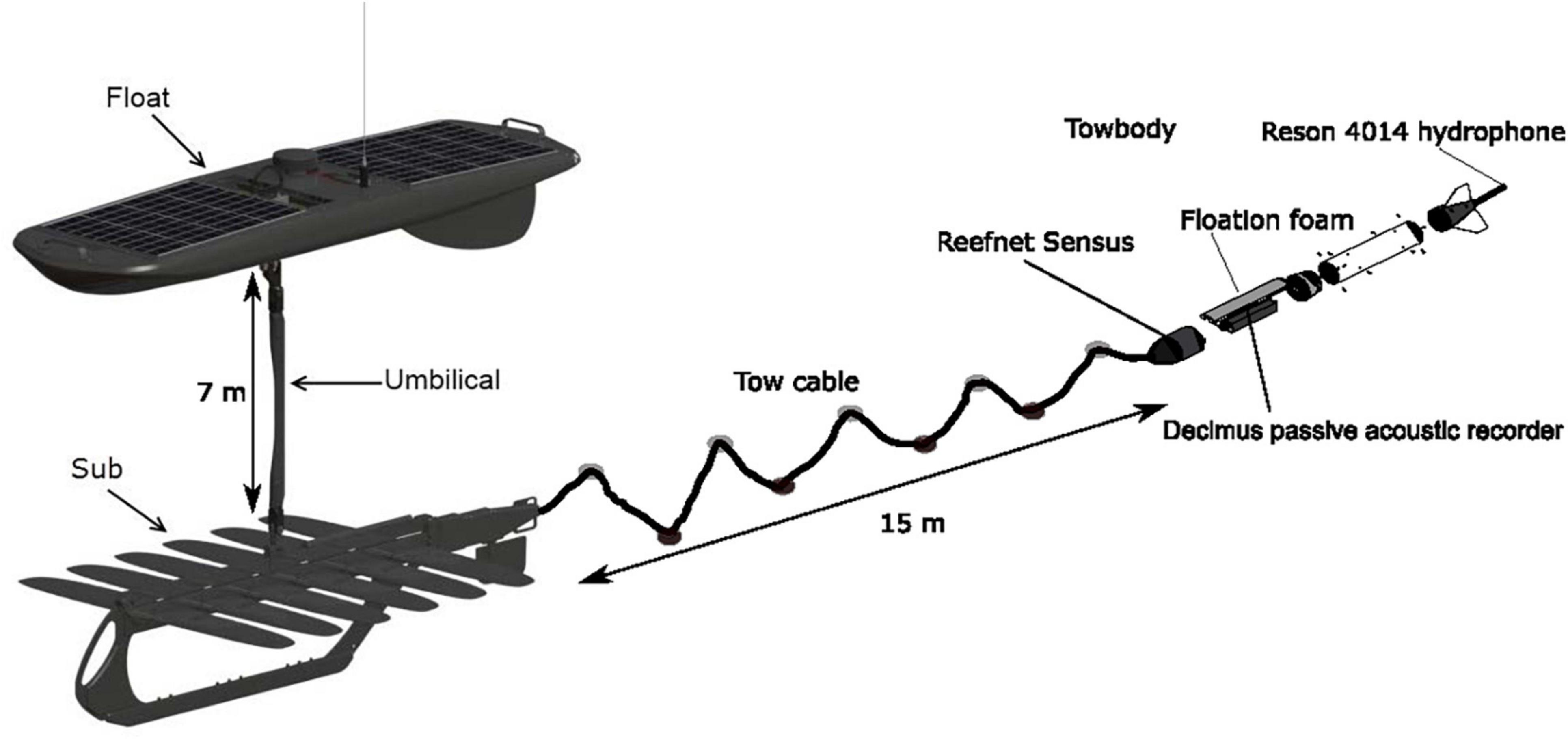
Figure 1. A diagram of the Acoustic Wave Glider (AWG), “Blackbeard,” showing the arrangement of instruments on the float (GPS and satellite antennae, solar panels, AIS antenna, weather station on mast, command and control box, fluorometer, acoustic doppler current profiler, and wave sensor), 7 m long umbilical, and glider instrumentation (CTD and acoustic tag receiver). The passive acoustic recorder and hydrophone system (Decimus) were towed on a 10 m cable with alternating floats and weights that help isolate the recording system from glider-generated noise.

During the deployment, the AWG was sent along a programmed sequential course for 9 days, reporting back to shore by satellite with AWG telemetry position data, current profiles, fluorometry measurements, text summaries of the passive acoustic data, wave data, and weather data. The towbody was attached to the submarine portion of the glider using a tow line containing alternating weights and floats to reduce the tension and minimize the transmission of vibrations from the glider to the hydrophone. The towbody was neutrally buoyant using the buoyancy adjustments as previously described (Luczkovich et al., 2019). Blackbeard towed the Decimus passive acoustic recorder behind the submarine portion of the glider at approximately 10 m meter depth without touching the bottom or colliding with any underwater reefs. The AWG was able to navigate in a southwesterly direction against the prevailing Gulf Stream current and return to navigate around artificial and natural reefs offshore in Onslow Bay, NC, United States (Figure 2). We recorded sounds continuously from August-01 13:39 (all times are local time UTC-4) to August-04 10:05 to observe variations in sounds throughout the diurnal cycle. Afterward, we recorded sounds only in the evenings to save energy (Table 1). Most soniferous fishes are primarily active at night (Luczkovich et al., 2008b; Pagniello et al., 2019) but see Nelson et al. (2011). The sound signal was measured from the calibrated hydrophone along the track of the wave glider in each mission.

TABLE 1

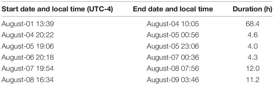
Table 1. Decimus passive acoustic start time, end time, and duration of recordings made on the wave glider survey.

FIGURE 2

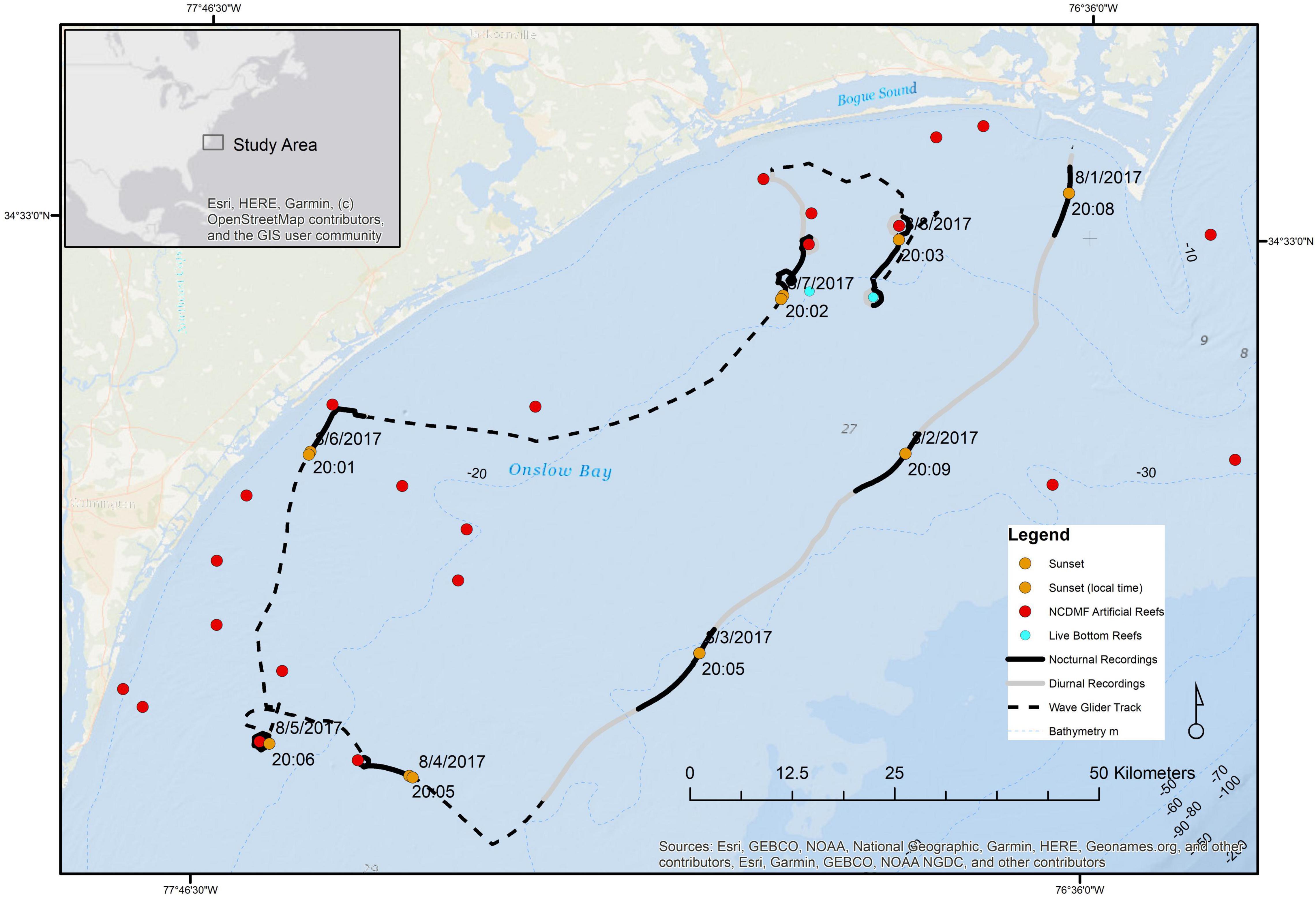
Figure 2. The track of the wave glider deployed August-01 through August-09 off North Carolina (United States) in Onslow Bay. The black dashed line shows the track of the wave glider, with nocturnal recordings shown as heavy black lines, and daytime recordings shown as gray lines, orange points show the position of the wave glider at sunset each day (in local time), the red points showing artificial reefs (North Carolina Artificial Reef Program, data source http://portal.ncdenr.org/web/mf/artificial-reefs-program), and cyan points showing live bottom reef areas. Bathymetry is in m, with 10 m contours shown as light bluedashed lines.

Previously, the SV2 wave glider was found to generate low levels of self-noise while towing a different passive acoustic recorder (HARP High-frequency Acoustic Recording Package), due to towbody cable strum and a servo motor that controls the rudder (Wiggins et al., 2010). The rudder servo-motor sounds are very brief (2 s) and broad-band (40 to 60 kHz) and do not mask low-frequency sounds made by biological sources like fish. The cable strum measured in that study was reduced by using a special tow-body fairing and re-designed tow cable (with alternating weights and floats) developed to allow a flexible coupling to the submarine, improvements incorporated into the current study wave glider and tow body design.

Sound Signal Analysis

We computed power spectra for each segment of the sound recordings. We used the power spectra to produce power spectral band sums (PSB sums) and composite spectrograms to identify recording segments for detailed analysis, consisting of listening to the recordings and creating spectrograms and power spectra of sounds of fishes and other sources. The reference power spectral density (PSD) used for all power spectrum levels in spectrograms was 1 μPa²/Hz and the reference band level for PSB sums was 1 μPa².

Power Spectra and Average Power Spectra

We divided each recording into overlapping 2048-point Hanning windows and computed power spectra. Each window overlapped the previous window by 1024 points (1/2 of the points). We computed average power spectra to produce PSB sums and composite spectrograms. We computed the average power spectra of identified fish sounds in the recordings using Hanning windows with the number of sample points chosen so the sample could be divided into at least four non-overlapping windows. Then we computed the average power spectrum using windows that overlapped by 1/2 of the window points for at least seven overlapping windows. This ensured that the sample points at the beginning and end of each sound that were reduced by the Hanning function were represented in either the previous or next overlapping window (Press et al., 2007). For computational efficiency, we used window sizes N_win that was a power of 2 such that the value of n as the largest integer such that

$N_{\text{win}}=2^n<\frac{N_{samp}}{4},(1)$

where N_samp is the number of sample points in the recording. The largest N_win we used was 2¹⁴ = 16 384 points, regardless of the length of the sample. The window size can be determined by

$\begin{array}{c}\hfill n=\lfloor {\text{log}}_2\left(\frac{N_{\text{samp}}}{4}\right)\rfloor ,\hfill \end{array}(2)$

where ⌊⌋ represents the floor function and the window size is N_win = 2ⁿ. For example, a 0.8 s recording sampled at 50,000 Hz contains 40,000 samples. An average power spectrum of this segment would use a window of N_win = 2¹³ = 8192 sample points because $\lfloor {\text{log}}_2\left(\frac{40,000}{4}\right)\rfloor =13$.

Spectrograms and Composite Spectrograms

Spectrograms of the recordings were produced with power spectral density (color axis) as a function of time (horizontal axis) and sound frequency (vertical axis). The fish sounds are in the lower frequency range (Table 2): at the low end, the red drum “knock” calls have a dominant frequency of 125 Hz; at the high end, the striped cusk-eel “chattering” calls are dominant at 1500 Hz, with a range of 1000 to 2500 Hz. Unless indicated otherwise, we produced spectrograms of shorter sounds (60 s or less) using 2048-point Hanning windows with overlaps of 1792 points. For sounds with short-time-duration features such as clicks and pulses, we used 512-point Hanning windows with overlaps of 448 points, sacrificing frequency resolution for increased time resolution. For time intervals longer than 3600 s (1 h), we produced composite spectrograms by averaging the power spectra described above for each 60 s in the recording and plotting the average power spectral density vs. time and frequency. We used a log₁₀ scale for the frequency axis for composite spectrograms to display both low- and high-frequency components in detail and used a linear scale frequency axis for species-specific spectrograms in which we display a limited frequency range. Harmonic frequency components, which are whole number multiples of the fundamental frequency, are easier to identify with a linear frequency scale because they are equally spaced in frequency.

TABLE 2

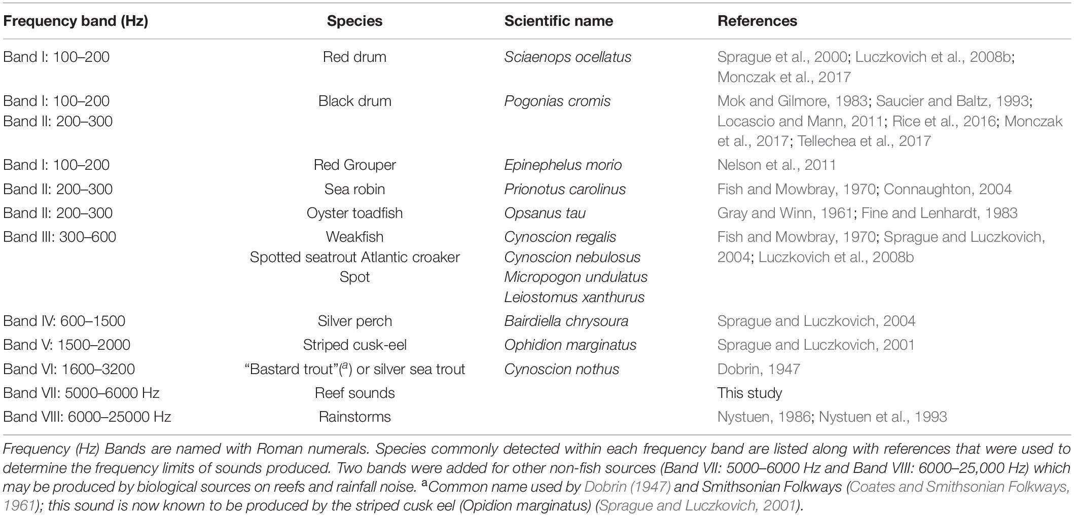
Table 2. Frequency bands were used to associate fish species and power spectral band sums.

Power Spectral Band Sums

We computed power spectral band sums (PSB sums) for specific frequency bands associated with known fish sounds. Table 2 shows the frequency range associated with different fish species. These frequency bands were chosen as indicators of calls by the various species. The bands do not contain all frequencies in the calls. A PSB sum S_PSB is the sum of all power spectrum components P_n for frequencies in the band f_min ≤ f_n ≤ f_max,

$\begin{array}{c}\hfill S_{\text{PSB}}(f_{\text{min}},f_{\text{max}})=S_{\text{PSB},n_{\text{min}}{n}_{\text{max}}}={\sum }_{n=n_{\text{min}}}^{n_{\text{max}}}{P}_n\mathrm{\Delta }f,\hfill \end{array}(3)$

where n_min is the index of the smallest frequency component in the band, n_max the index of the largest frequency component in the band, and Δf the frequency interval in the power spectrum.

We computed the average PSB sum of each band in Table 2 for each 60 s of the recording and plotted them vs. time to identify times in the recordings likely to contain fish sounds. One indication of fish activity is when the PSB sum for a frequency band increased with a different pattern than the other bands. For example, if the 100 to 200 Hz PSB sum increased by 20 dB while the other bands remained the same, the recording was likely to have black drum, red drum, or grouper sound production (Table 2), or it could have had noise produced by ships that also has frequency components within that band. Note that a PSB sum value cannot positively identify a sound source, but it can eliminate portions of a recording unlikely to contain calls with frequencies within the band. We listened to and analyzed each identified region in detail to identify individual fish calls and aggregation sounds.

Pulse Period and Pulse Repetition Rate

The pulse period and pulse repetition rate for calls in a fish chorus are often difficult to measure because a recording may have many individual calls at the same time causing difficulty in isolating pulses in a call from the same source. We measured the pulse period for the example species pulsed calls when we were confident that a pulse train in the call was from one individual. We measured the pulse period using the times between similar features (e.g., peaks) in the oscillogram for consecutive pulses. When the oscillogram was not clear due to noise in other frequency bands, we filtered the signal using a second-order section digital implementation of a 20th order Butterworth bandpass filter that included all significant frequencies in the average power spectrum. We report the mean pulse period and use the standard error of the pulse period as the uncertainty. We calculated the pulse repetition rate as the reciprocal of the pulse period.

Sound Pressure Levels and Frequency Band Sound Pressure Levels

We calculated sound pressure levels (SPLs) and frequency band sound pressure levels to compare our recordings with those made by other researchers. We calculated RMS sound pressures from sampled sounds using

$\begin{array}{c}\hfill p_{\text{RMS}}\left(t_n\right)=\frac{\mathrm{\Delta }t}{T}{\sum }_{i=1}^n{p}_i^2{e}^{-\frac{t_n-t_i}{T}}\hfill \end{array},(4)$

where t_n is the time of sample n, Δt the sample interval, p_i the pressure at sample i, and T the time constant. Eq. 4 approximates the integral used to calculate average RMS pressures for analog signals. We used a time constant of T = 0.125 s for “fast” response measurements and T = 1.00 s for “slow” response measurements. We calculated SPLs from the band RMS sound pressure with

$\begin{array}{c}\hfill L\left(t_n\right)=20{\text{log}}_{10}\left(\frac{p_{\text{RMS}}\left(t_n\right)}{1\mathrm{\mu }Pa}\right).\hfill \end{array}(5)$

We calculated frequency band SPLs by using a second-order section digital implementation of a 20th order Butterworth bandpass filter set to the minimum and maximum frequencies of the band. Then we used the band-filtered pressure samples in Eq. 4 to obtain band-filtered RMS pressures, which we used in Eq. 5 to obtain frequency band SPLs.

Sound Source Identification

We listened to a selection of recorded files based on the increased levels of the various PSB sums. When a PSB sum band increases, there is a sound source that causes that increase by producing frequencies within the band. Listening to the sounds allowed us to identify sources causing the PSB increases. We used Raven Pro Bioacoustics software (Center for Conservation Bioacoustics, 2019) to playback the recordings, listen to and select parts of the soundscape for identification using oscillograms, spectrograms, and power spectra. A scrolling spectrogram in Raven was observed by a listener and selection boxes were established around each sound to be identified for further spectral analysis.

Mapping Procedures

Interpolation of the PSB sums was computed in ArcMap 10.6.1 (www.esri.com, ESRI, Redlands, CA, United States) and used to generate maps of the power spectral density along the wave glider track. First, a 500 m buffer was generated around the wave glider path, which was imported from points obtained at 300 s (5 min) time intervals, with coordinate positions reported via the Wave Glider Management System and then converted to a line in ArcMap. Next, the Kernel Interpolation with Barriers Tool in the Geostatistical Analyst Toolbox in ArcMap was used to create a prediction surface for the PSDs at each 10 m cell with the 500 m buffer zone. The kernel interpolation used the point values of PSB sums for the full spectrum to produce a raster prediction surface. A final map of each fish chorus type as defined by PSB sums in each fish species-specific frequency band (Table 2) that exceeded the 90th percentile for all sums was produced along the wave glider track as a way of visualizing each fish chorus linear extent. The values for each PSB sum Band were imported into the statistical package R to compute the 90th percentiles (R Core Team, 2021). Values that exceeded these percentiles were converted from points to lines and plotted on the map.

Results

Fish Choruses in the Soundscape

Upon recovery, the recorded sounds from this mission were analyzed using composite spectrograms and PSB sums associated with different fish species (Table 2). The first set of soundscape recordings was made along continuously changing depth profiles to examine variations in the soundscape between day and night as the wave glider moved from inshore at 10 m depth to offshore 27 m (Figure 2). During this time, the passive acoustic system in the tow body averaged 11 m depth and the temperature was 26.3°C. The PSB sum plots (Figure 3A), and the composite spectrogram (Figure 3B) display variations in the soundscape as the wave glider moved along the track. Four of the PSB sums (Band I 100 to 200 Hz, Band III 300 to 600 Hz, Band V 1500 to 2000 Hz, and Band VII 5000 to 6000 Hz) show increases that are not reflected in the other band (Band VIII 6500 to 25000 Hz) between the night hours of 16:00 and 02:00 (Figure 3A). Between 2017-August-01 from 19:55 (just before sunset at 20:08) until midnight, there is a fish chorus visible in the composite spectrogram (Figure 3B) dominating the low- and mid-frequency power spectral bands (with the greatest contribution > 100 dB re 1 μPa² in the 300 to 600 Hz band; Figure 3A). This increase in the 300 to 600 Hz PSB sum is due to multiple species of Sciaenidae including weakfish C. regalis, Atlantic croaker Micropogonias undulatus, and an unknown species producing a 500 Hz “grunt,” likely to be a member of the Sciaenidae. This is what we term the Sciaenidae mixed-species chorus (dominating Bands I and III; description below), which, at its peak, exceeded a band level of 120 dB re 1 μPa². This chorus grew in amplitude as the wave glider progressed offshore, occurred in water depths of 17 to 19 m, reached the peak in Band III of 124 dB re 1 μPa² at 21:57, and diminished to <100 dB re 1 μPa² at August-02 00:34.

FIGURE 3

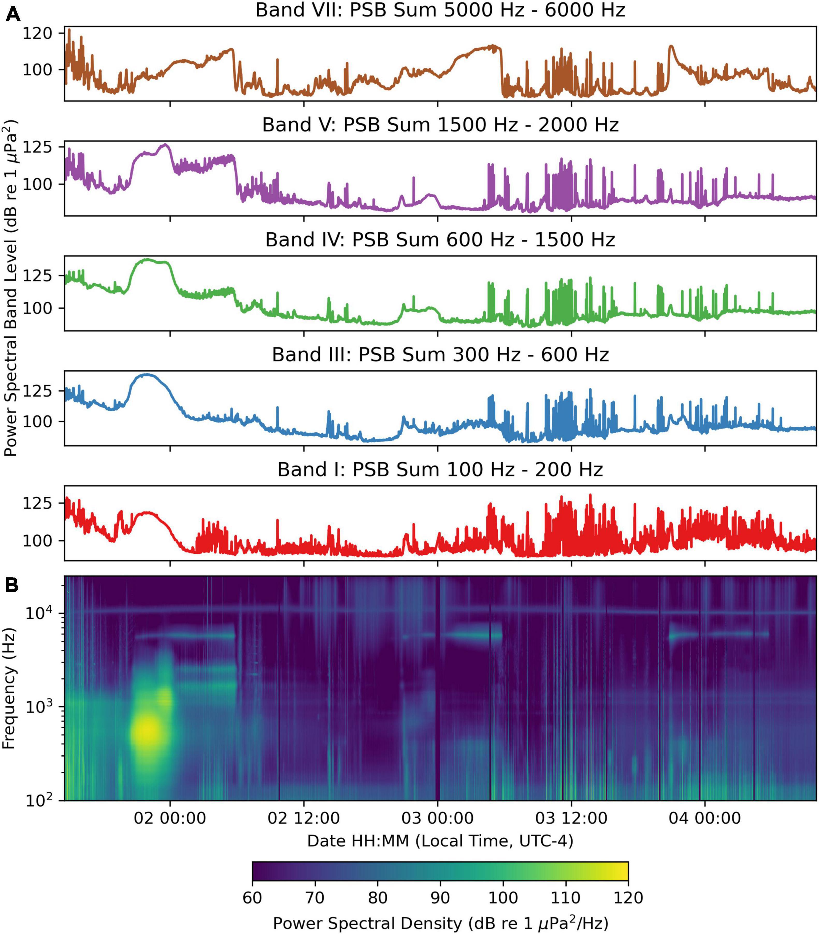
Figure 3. Sound recorded continuously by the wave glider Blackbeard between August-01 and August-04. (A) Power spectral band sums for 60 s windows of the recording. (B) Composite spectrogram produced from 60 s average power spectral densities.

Diurnal and Nocturnal Variability in the Soundscape

Although we cannot directly compare daytime and nighttime variation at a single geographical position, as many have done with fixed position passive acoustic recorders, nonetheless, during each 24 h period the sounds recorded by the moving hydrophone were much lower in the daytime than at night after sunset. This was most noticeable in Band I (100 to 200 Hz), Band III (300 to 600 Hz), Band V (1500 to 2000 Hz), and in Band VII (5000 to 6000 Hz), but not above 6000 Hz during the first day and night (August-01 12:00 to August-02 12:00, Figure 3). The composite spectrogram is shown in Figure 3B, and these PSB sums vary in concert with the brightest areas in the spectrogram. Upon listening to these recordings from daytime through the evening on August-01, the overall PSB sum in Bands I, II, and III increased. One could hear first vessel noise, then individual fish calls increasing, then decreasing, in amplitude as they were passed by the wave glider as it moved offshore. On August-01 20:25, one can hear a mixed chorus of weakfish “purrs,” the unknown Sciaenidae “grunts” occurring along with occasional striped cusk-eel “chatters” all together in 130-s sound clip (Supplementary Figure S1, Sound Clip Audio 1). Later in the time series, from just before midnight on August-02, as the wave glider was further offshore and in deeper water, the 1500–2000 Hz band increased and the 300 to 600 Hz band further declined (Figure 4A). This is evidence of a different type of fish chorus (Figure 4B, spanning PSB sums Band III, Band IV, and Band V), produced by both the unknown “grunt” and the striped cusk-eels O. marginatum (Ophidiidae), that dominates the soundscape (see Ophidiidae chorus description below). It occurred in water depths of 17–20 m and diminished <95 dB 1 μPa² at August-02 05:51. The peak PSB sum (>105 dB 1 μPa²) of Band V was between August-01 21:11 and August-02 01:44. These two fish choruses overlap during the post-sunset hours (from August-01 at 20:34) until the early morning as the Sciaenidae Chorus in Band III stopped calling. These two choruses occur in separate frequency bands, and the period of overlap is visible in the composite spectrogram (Figure 3B) on the first night of the recording. We computed a PSB sum in Band IV for detection of the unknown grunt, which we had previously associated calls in this frequency range with a different member of the Sciaenidae, the silver perch Bairdiella chrysoura. We never heard silver perch in these recordings, so we do not know which species made this sound, but Band IV was displayed on the graphs in Figure 4, and it matches well temporally with the unknown grunt chorus.

FIGURE 4

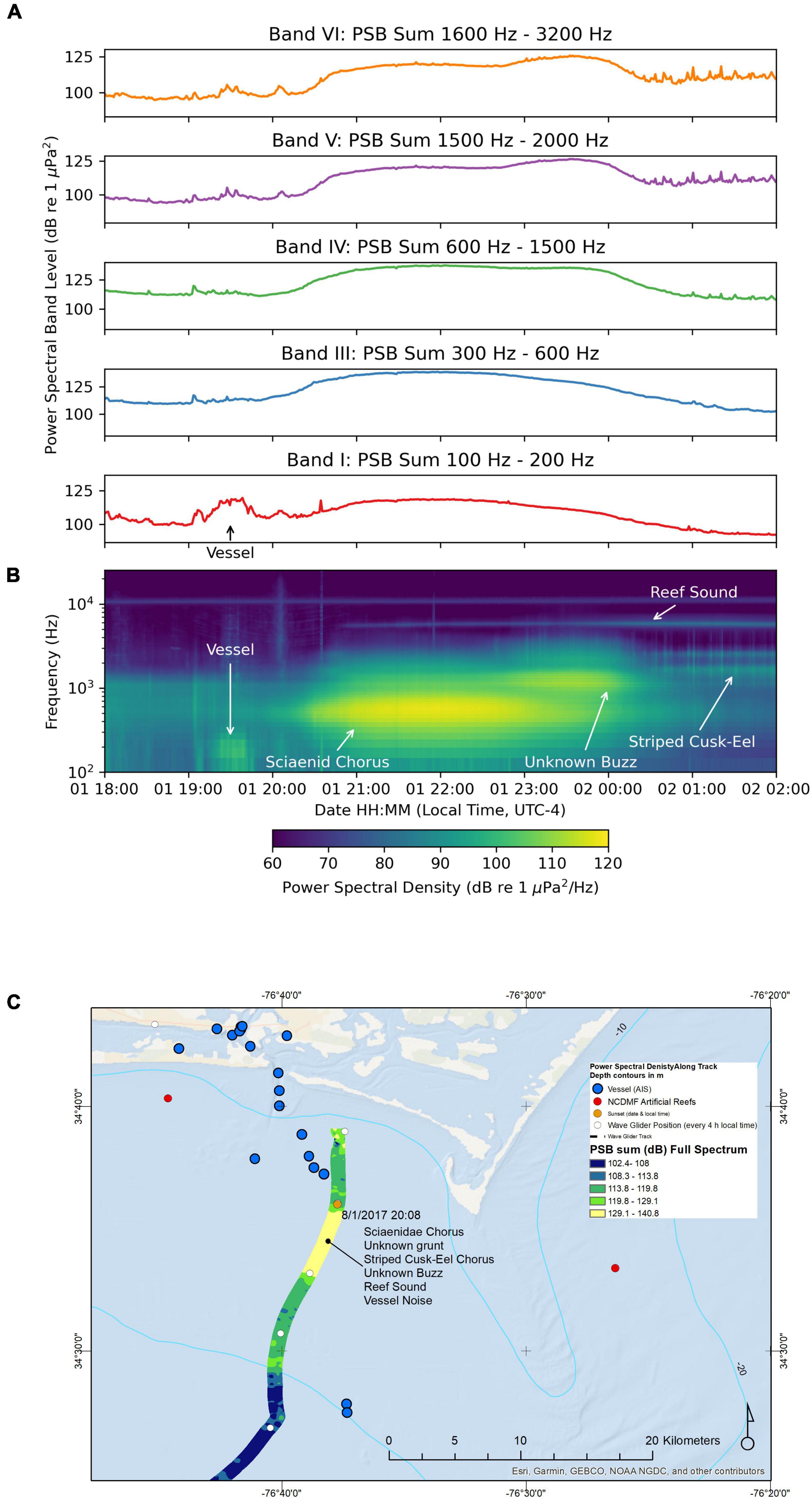
Figure 4. Sound recorded by the wave glider Blackbeard between August-01 18:00 and August-02 02:00. (A) Power spectral band sums for 60 s windows of the recording. (B) Composite spectrogram produced from 60 s average power spectral densities. (C) Map of the path of the wave glider during the recording. The color of the path indicates the full spectrum PSB sum detected at the location.

We also recorded on these nights a band of energy at 5600 Hz, which is reflected in the 4000 to 10,000 Hz PSB sum plot; we believe this band (Band VII) to be associated with a live bottom reef area (see Section “Reef Sound description” below). During the following daytime period on August-02, all PSB sums drop to low levels (80–90 dB re 1 μPa²). On subsequent nights, presented in the next several sections, the dominant Sciaenidae chorus 300 to 600 Hz (Band III) was no longer present in the deeper waters (20 to 30 m), but the 100–200 Hz Band I increased slightly, and the other chorus (Band V cusk-eels) and reef sounds (Band VII 5000 to 6000 Hz) remain. After August-04 we made recordings during the night only. In the next section, we examine each of these nocturnal choruses in greater detail.

Nocturnal Soundscape on August-01 and August-02

Recordings were made on this transect inshore between Cape Lookout and Beaufort Inlet in water 13–18 m deep with a water temperature of 26.3°C (Figure 4C). The hydrophone on the towbody averaged 11 m deep. Vessels departing the port in the Beaufort channel were received by the wave glider’s Automatic Identification System (AIS) receiver in this area, ranging from small fishing vessels (10 m) to a large (179 m) cargo vessel in the ship channel 5.4 km away, which contributed to the soundscape between 19:00 and 20:00 as it passed by. This large vessel was visible as a rise in the 100 to 200 Hz PSB sum (Figure 4A) and the composite spectrogram (Figure 4B). Figure 4C shows a map of the vessel’s AIS signals received along the wave glider’s track, plotted with variations in the soundscape, interpolated using the full-spectrum PSB sums; this map indicates where the fish choruses and anthropogenic noises from the vessel were loudest. The noise from the large cargo vessel passing close to the wave glider hydrophone was not as loud as the fish choruses (Figure 4) to be encountered a little later.

After 20:08 (sunset, indicated on the map in Figure 2), we can see an increase in PSB sum values in Bands I–VI (Figure 4A) due to fish choruses. The first chorus encountered was the Scianeidae mixed-species chorus in Bands III and IV; the next chorus was due to a “buzz” sound made by an unknown species in Bands V and VI; the third chorus was due to striped cusk-eels (in Band V). Sounds identified in the first Sciaenidae chorus by a listener were the weakfish C. regalis, Atlantic croaker M. undulatus, and an unknown “grunt” suspected to be a member of the Sciaenidae, and striped cusk-eels O. marginatum. The Sciaenidae mixed-species chorus persisted from 20:08 until midnight with PSB sum values exceeding 120 dB re 1 μPa² in Bands III and IV when the unknown “grunt” call was dominant. The Band III PSB sum peaked at 138 dB re 1 μPa² at 23:33. The chorus of unknown “buzz” calls began to increase in amplitude around 23:00 and continued to increase as the Sciaenidae mixed-species chorus began to fade around 23:30. The Band VI PSB sum reached a peak value of 126 dB re 1 μPa² at 23:32 and began to decrease after midnight. The striped cusk-eel chorus that followed had PSB sum values in Bands V and VI that rose and fell as the wave glider passed clusters of calling individuals. The peak Band VI PSB sum during the striped cusk-eel chorus was 118 dB re 1 μPa² on August 2 at 01:20, and the peak Band V PSB sum during the same chorus was 117 dB re 1 μPa² at the same time.

In addition to PSB sums, we measured SPLs for comparison with sounds measured in other studies. We measured the maximum fast time constant SPL of this entire survey, 148 dB 1 μPa, on this night at 21:54:47 as the wave glider passed close to an individual fish making the unknown “grunt” call.

Nocturnal Soundscape on August-02 and August-03

Figure 5A shows the PSB sums and Figure 5B shows a composite spectrogram for the recordings made between August-02 18:00 and August-03 02:00 as the wave glider passed over the deepest water surveyed (25 to 27 m), while the hydrophone on the towbody was averaging 12 m deep. The water temperature at that depth was 26.5°C. Because of this greater depth and distance between the bottom and the hydrophone, we recorded lower overall sound levels here, due to fishes producing the sounds being in deeper water. There are peaks in the Band III PSB sum and the Band I PSB sum near the time 21:00. There is a gap in the recording between August-02 23:48 and August-03 00:10 due to an unexpected reboot of the recorder.

FIGURE 5

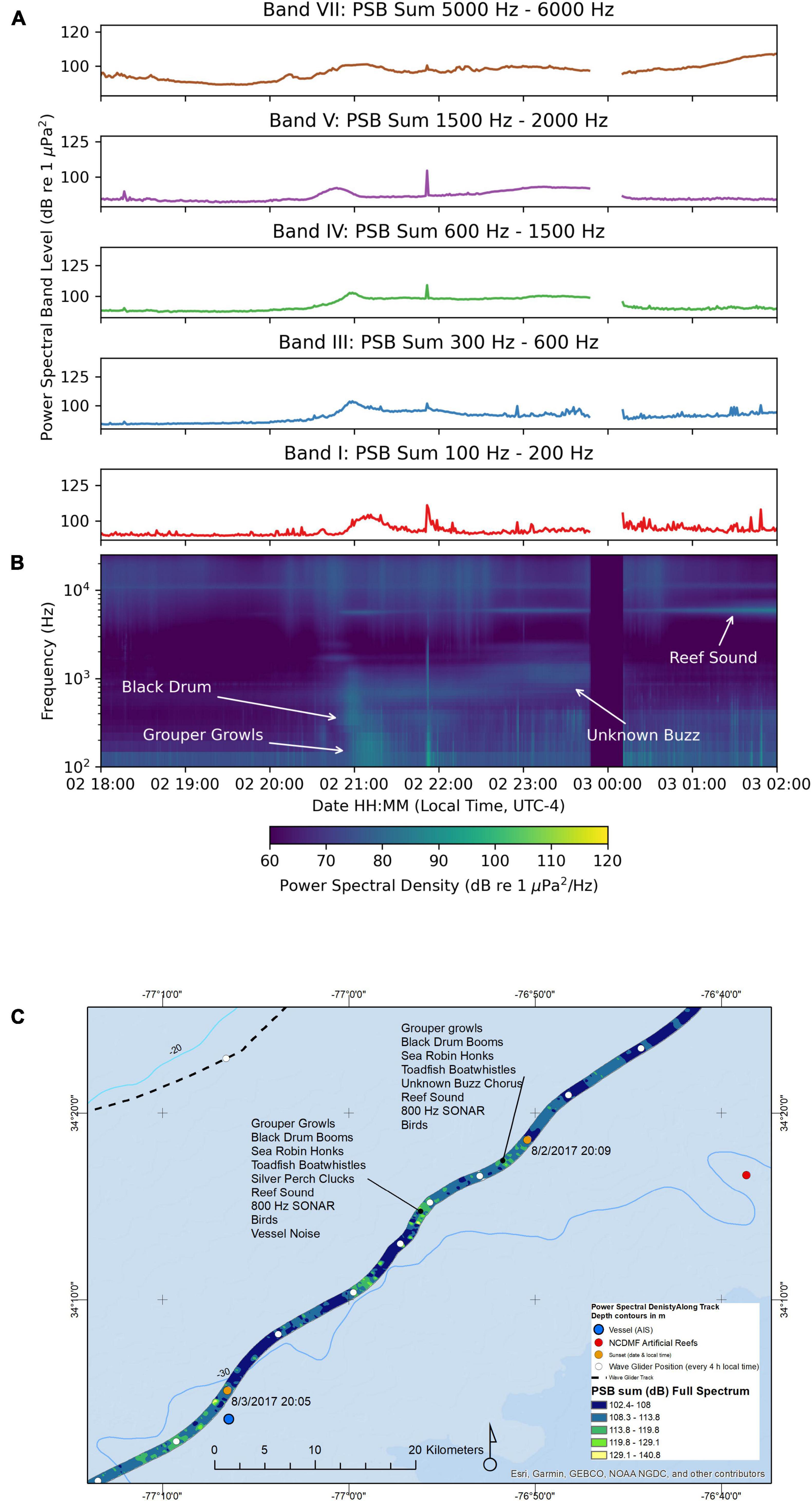
Figure 5. Sound recorded by the wave glider Blackbeard between August-02 18:00 and August-03 0:00. (A) Power spectral band sums for 60 s windows of the recording. (B) Composite spectrogram produced from 60 s average power spectral densities. The gaps in the plots were due to the recording system being rebooted, and thus no data were obtained during this time. (C) Map of the path of the wave glider during the recording. The color of the path indicates the full spectrum PSB sum detected at the location.

There was a notable absence of the loud Sciaenidae (Band III) and striped cusk-eel chorus (Band V) from the previous night (Figure 5A). There was an increase at points along this path in the Band I (100 to 200 Hz) and Band III (300 to 600 Hz) PSB sums (Figure 5A). The PSB values were low, <100 dB re 1 μPa².

Individual calls of fishes of several species were discernable. Oyster toadfish “boatwhistle” sounds, grouper “growls,” black drum “booms,” and sea robin “honks” were detected along this path (Figure 5C). The grouper “growls” caused the Band I PSB sum to increase. Grouper “growls” have been described for red grouper (Epinephelus morio) and spectral analysis of our growls are similar to growls reported for red grouper, but we did not identify the species of grouper based on the spectral analysis, as there are fishery reports of other species in that area, notably the gag grouper (Mycteroperca microlepis). We recorded what we believe to be reef sounds at 5600 Hz. Many live bottom reefs occur in the Onslow Bay at this depth, most of them are not accurately charted. These reef sounds occurred each night and were not present along the entire track of the wave glider in the daytime. This reef sound can be observed on the Band VII PSB sum plot for 5000 to 6000 Hz.

A persistent droning sound was present during the entire night in this section, which we conclude was a distant chorus of fish species making the unknown “buzz” sound, although individual fish calls could not be discerned. This identification was based on the similar spectral characteristics of sound to the unknown “buzz” call (1000 to 2000 Hz) from the previous night.

Finally, we recorded rainfall sounds during this night, which were audible on the recordings and can be seen as broad-spectrum sounds from Band VIII (6500 to 25,000 Hz) in the spectrogram (Figure 5B and Supplementary Figure S11, Sound Clip Audio 14). Peaks in the 6500 to 25,000 Hz PSB sum occur during rainstorms.

Nocturnal Soundscape on August-06 and August-07

Figure 6 shows the PSB sums (Figure 6A) and a composite spectrogram (Figure 6B) for the recordings made between August-06 18:00 and August-07 02:00. During this evening the sound recorder was on from August-06 20:16 to August-07 00:42. The PSB sums for this segment increased in Band I (100 to 200 Hz). The wave glider path was near New Topsail Inlet inshore with multiple North Carolina Division of Marine Fisheries (NCDMF) artificial reefs near the path (Figure 6C). Along this path, the wave glider recorded sounds in 13 m deep water, while the hydrophone on the tow body was 9 m deep, and the water temperature was 27.5°C. Species and sounds heard on this nocturnal recording include the Sciaenidae chorus, which was dominated by the unknown grunt call (500 Hz), weakfish, striped cusk-eels, reef sounds, and rain with thunder. We recorded a maximum fast time constant SPL of 142 dB re 1 μPa on this night at 21:31:19 with all of these species chorusing and the rainstorm and thunder sound adding to the soundscape.

FIGURE 6

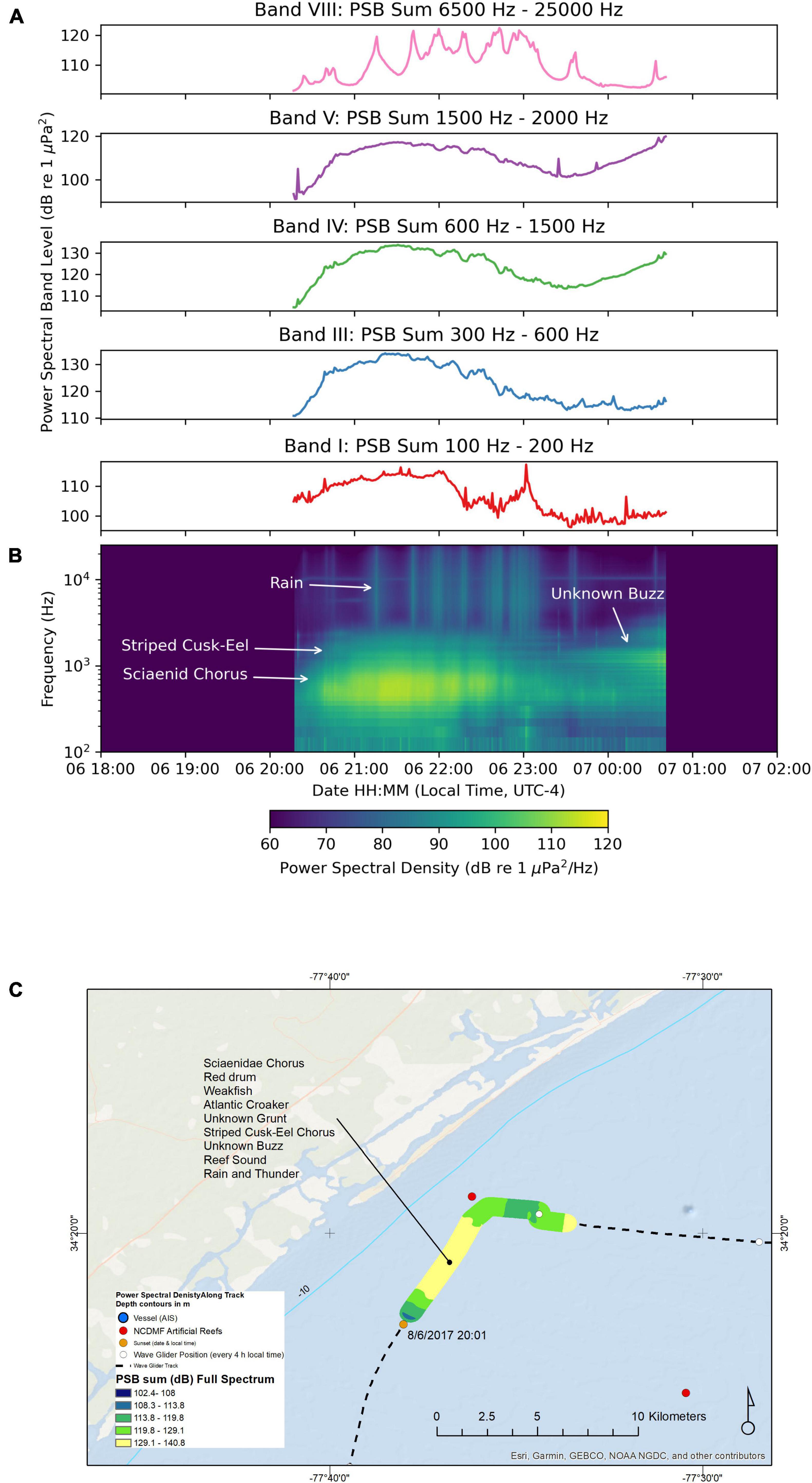
Figure 6. Sound recorded by the wave glider Blackbeard between August-06 18:00 and August-07 02:00. (A) Power spectral band sums for 60 s windows of the recording. (B) Composite spectrogram produced from 60 s average power spectral densities. (C) Map of the path of the wave glider during the recording. The color of the path indicates the full spectrum PSB sum detected at the location.

Nocturnal Soundscape on August-07 and August-08

On this night, we sent the wave glider on a circular path around an area with no NCDMF artificial reef as a control (we did not anticipate a reef to be at this location) and then on a circular path around an NCDMF artificial reef (Figure 7). Along this course, the wave glider recorded sounds in 17 to 20 m deep water, while the hydrophone on the tow body was 8 m deep and the water temperature was 27.1°C. The PSB sums for all bands were generally lower than other nights (August-01 and August-02 Figure 4A; August-06 and August-07 Figure 6A) at a similar water depth, ranging between 100 and 120 dB re 1 μPa² with occasional spikes indicating nearby calling fishes (Figure 7A). The composite spectrogram indicated the presence of low-frequency red drum calls and higher-frequency striped cusk-eels, nocturnal reef sounds, then later the unknown “buzz” sound (Figure 7B). Individual fish calls could be heard by a listener as the wave glider passed nearby these calling individuals. Species identified on the recordings included red drum, black drum, striped cusk-eels, the unknown “buzz,” and the 5600 Hz reef sound. As it turned out later, after the mission was over, we learned from fishers that there was a natural live bottom reef close by the orbit around the non-artificial-reef control path (Figure 7C). Hence, the 5600 Hz sound was associated with a natural live bottom reef here.

FIGURE 7

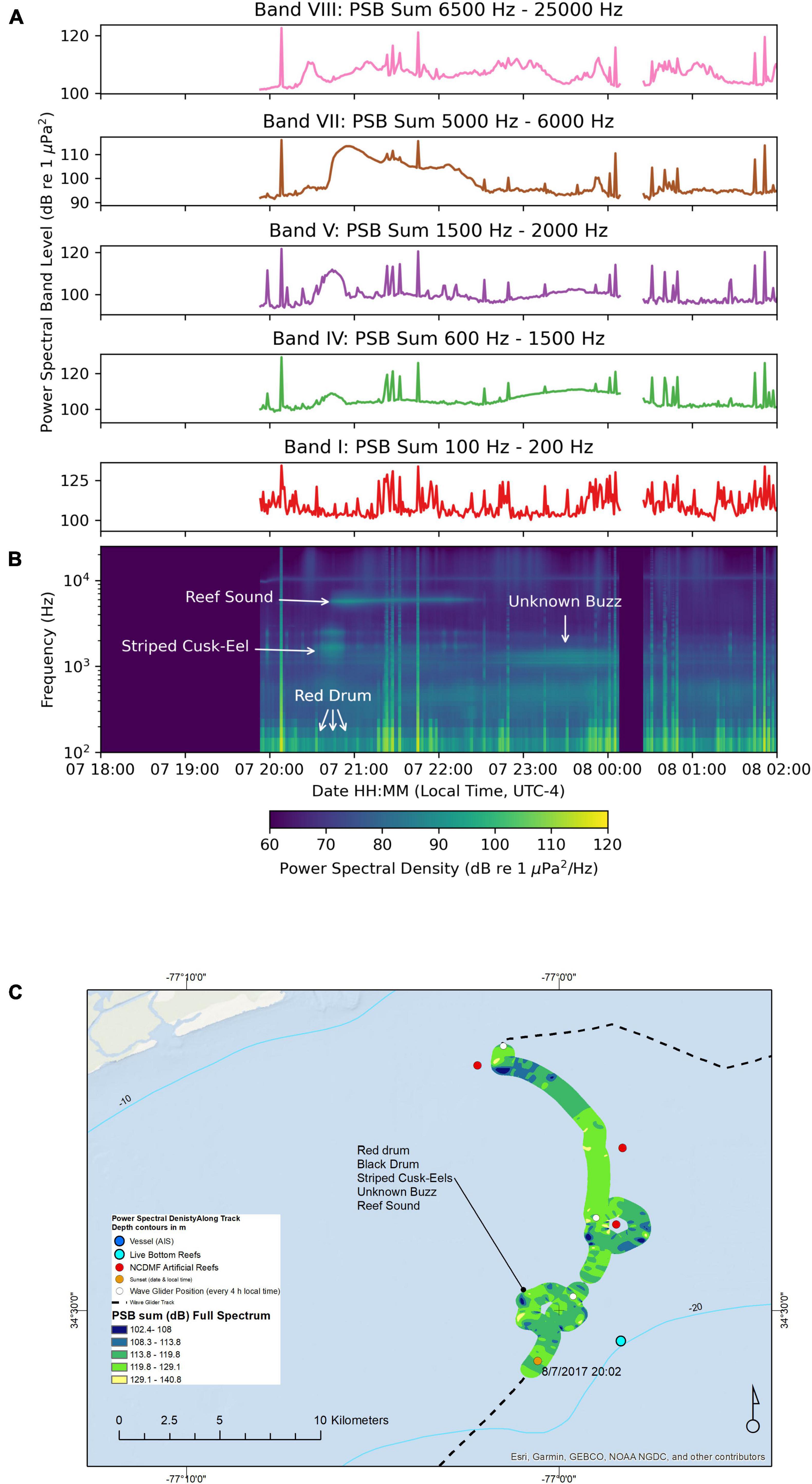
Figure 7. Sound recorded by the wave glider Blackbeard between August-07 18:00 and August-08 02:00. (A) Power spectral band sums for 60 s windows of the recording. (B) Composite spectrogram produced from 60 s average power spectral densities. The gaps in the plots were due to the recording system being rebooted, and thus no data were obtained during this time. (C) Map of the path of the wave glider during the recording. The color of the path indicates the full spectrum PSB sum detected at the location.

Nocturnal Soundscape on August-08 and August-09

The path took us past both and an artificial reef and a natural live bottom area for an intended comparison (Figure 8). Along this path, the wave glider recorded sounds in 17 to 22 m deep water, while the hydrophone on the tow body was 9 m deep and the water temperature was 27.1°C. Similar to the previous night (August-07 and August-08), the PSB sums in each band were lower than the maximum PSD sums observed on August-01 and August-02, but still were in the range 100 to 120 dB re 1 μPa². The loudest striped cusk-eel chorus in Band V with a PSB sum value 119 dB re 1 μPa² occurred on August-08 at 20:35:03 just after sunset (Figure 8A). The composite spectrogram showed spectral characteristics typical of red drum, black drum, striped cusk-eels, reef sounds, the unknown “buzz” sound, and a Sciaenidae mixed-species chorus (Figure 8B). Listeners confirmed these species based on individual calls heard along this track: black drum (Band I and II), red drum (Band I), a mixed Sciaenidae chorus (Band III) dominated by the unknown “grunt,” and the unknown “buzz” (Band VI). The map of the path around the artificial and natural reefs is shown with the full spectrum PSD sum plotted along the path (Figure 8C). This clockwise circle of the artificial reef happened before sunset (20:08). It is important to note the time when the wave glider passed by each reef in this plot: the wave glider approached the artificial reef on this course from the north, beginning the circle of the artificial reef at 14:33, traveling along the eastern arc of the circle in a clockwise manner, reaching the southern edge of the circle at 16:18, then heading around the western edge of the circle until 17:48, then retracing the eastern circle path until 19:48. Next, the wave glider headed SSW on a path reaching the north edge of the circle path of the natural live bottom just after midnight 00:38 on August-09. The wave glider circled the natural reef in a clockwise path until 03:43. Thus, these two orbital paths took ∼3 h to complete and were not done during a similar part of the diurnal cycle of the soundscape for each reef. Thus, a direct comparison of an artificial reef and natural reef soundscape at the same time of the night was not possible in this study, because of the temporal variation in fish calling that occurred during the night.

FIGURE 8

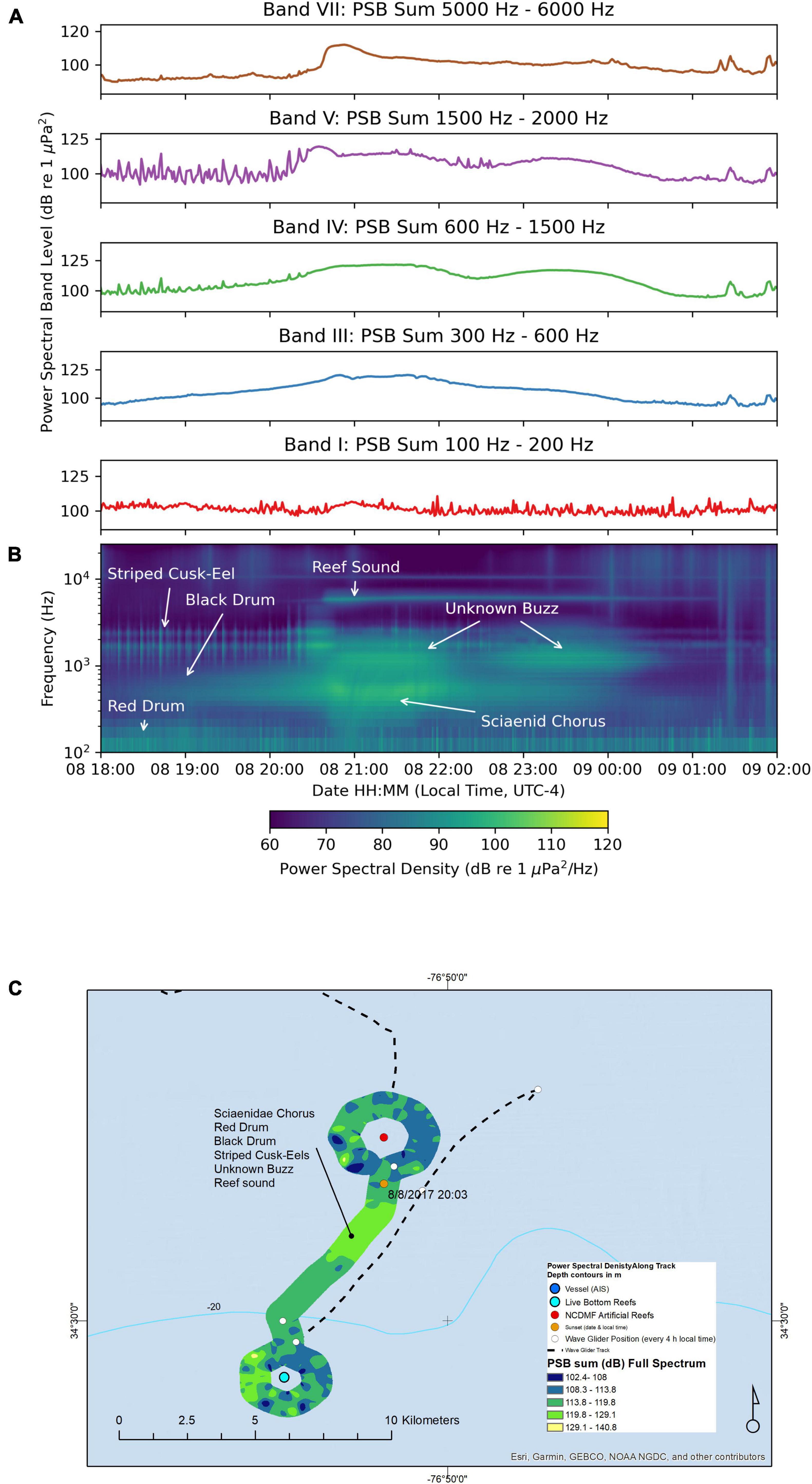
Figure 8. Sound recorded by the wave glider Blackbeard between August-08 18:00 and August-09 02:00. (A) Power spectral band sums for 60 s windows of the recording. (B) Composite spectrogram produced from 60 s average power spectral densities. (C) Map of the path of the wave glider during the recording. The color of the path indicates the full spectrum PSB sum detected at the location.

The peak PSB sum for the full spectrum occurred as the wave glider traveled between the two reefs, in the hours after sunset (20:08) through midnight, as was typical elsewhere in our survey. The nocturnal reef sound appeared in the composite spectrogram (Figure 8B) while the wave glider was between the artificial and natural reefs after sunset, and appears to get less intense as it approached the natural reef at midnight. A listener identified individual species calls on the recordings: red drum, black drum, and striped cusk-eels calls peaked while the wave glider was circling the artificial reef area before sunset. The Sciaenidae chorus and the unknown “buzz” chorus were at their respective peaks in between the artificial reef and the natural reef area, after sunset and before midnight on August-08. The live bottom reef thus had less intense chorusing after midnight through 03:43 on August-09.

This type of temporal variation was typical for the fish choruses. If we compare the soundscape on the circle near the natural live bottom reef August-07 at 20:22 through midnight (Figure 7B) with the artificial reef August-08 at the same time (Figure 8B), we see red drum, black drum, and striped cusk -eel choruses in both composite spectrograms. Likewise, if we compare the soundscape of the circle around the artificial reef 08-August at 01:08 through 03:42 (Figure 7B) with the circle around the natural reef at the same time on 09-August (Figure 8B), there are unknown buzz choruses and Sciaenidae choruses in both spectrograms. These choruses occur in the soundscape in the same temporal order on successive nights. It is not dependent on whether there are artificial or natural reefs nearby.

Soundscape Description

In the following sections, we describe the sounds that comprised the soundscape during specific stretches of the wave glider path. Some sounds could be identified as known soniferous (sound-producing) species including red drum (S. ocellatus), black drum (Pogonias cromis), weakfish (C. regalis), Atlantic croaker (M. undulatus), oyster toadfish (O. tau), searobin (Prionotus sp.), and striped cusk-eel (O. marginatum); these identifications were done using audio sound clips, spectrograms, and average power spectrum plots that are provided in Supplementary Datasheet 1 and Supplementary Sound Clip Audios 5–12; other sounds could not be associated with known species, and spectrograms, average power spectra, and descriptions of these unknown sounds are provided below.

Grouper “Growl” Description

The recordings contain “growl” calls produced by grouper species shown in Figure 9 and Supplementary Sound Clip Audio 2. Figure 9A shows a spectrogram of a 15 s recording segment containing two “growl” calls. Figure 9B shows a spectrogram of the second call, and Figure 9C shows an average power spectrum of the same call and of the background noise, which likely contained other “growl” calls in the distance. The “growl” call in Figure 9B and C has a dominant frequency of 125 Hz with other prominent peaks at 88, 107, 180, 195, and 287 Hz. We filtered the waveform using a 50 to 750 Hz bandpass filter and were able to identify two sets of four pulses in the oscillogram that likely came from the same individual. These pulses had a period of 0.056 ± 0.001 s and a pulse repetition rate of 17.9 ± 0.4 Hz.

FIGURE 9

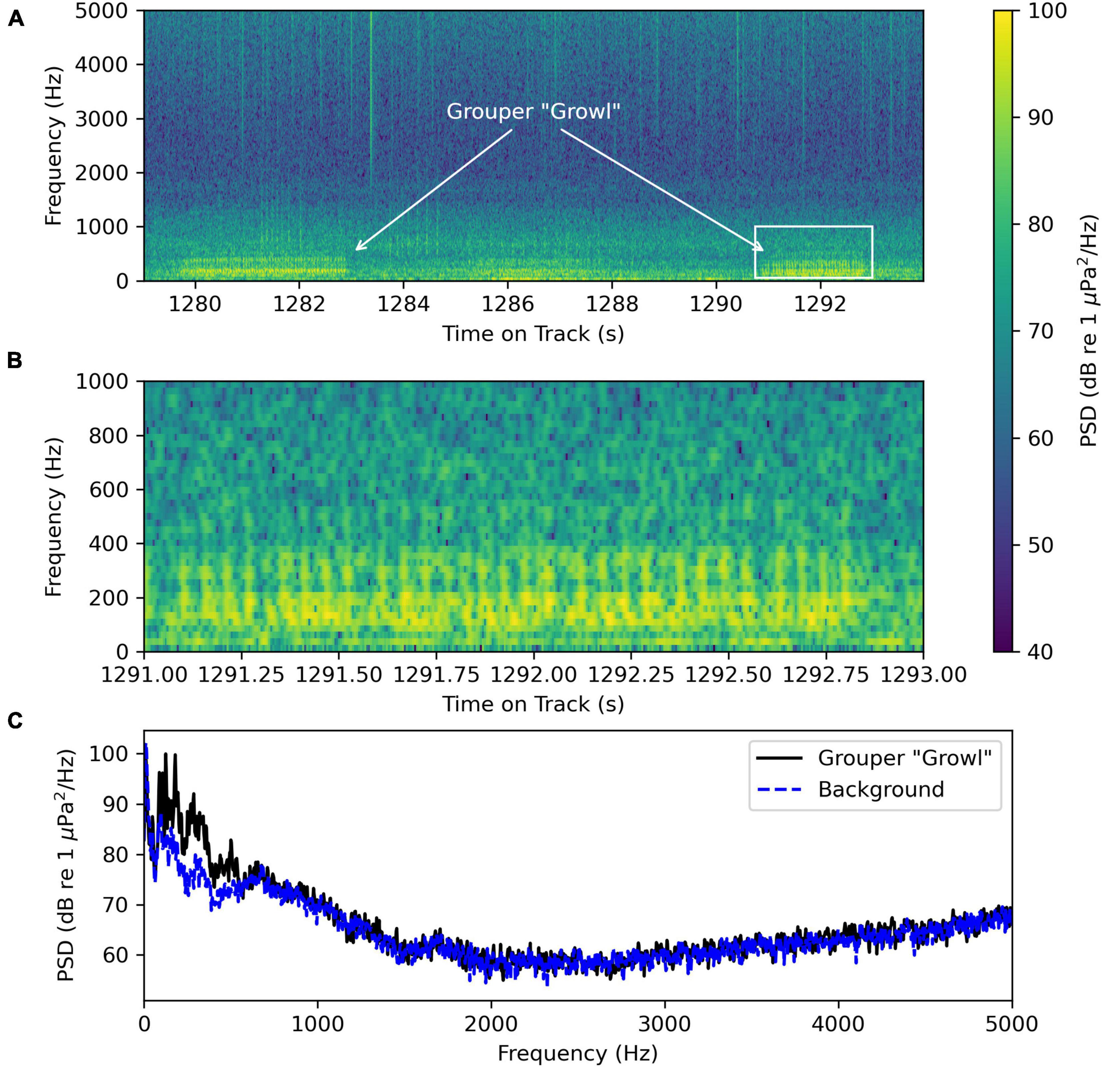
Figure 9. Grouper “growl” sounds recorded by the wave glider Blackbeard at August-07 20:56:05 at latitude and longitude (34.494 632N, 77.009 573W). (A) Spectrogram of a 15 s segment of the recording containing two distinct “growl” sounds. (B) Spectrogram of the second “growl” sound in panel (A) outlined in the rectangle. (C) Average power spectrum for the “growl” sound shown in panel (B) from 1291.0 to 1293.0 s in the recording and the background noise from 1288.0 to 1290.5 s when there were no “growl” sounds detected. Both average power spectra were computed using 16 384-point Hanning windows with an overlap of 8192 points.

Unknown “Grunt” Description

The recordings contain unknown “grunt” calls likely to be produced by a Sciaenidae species (Figure 10 and Supplementary Sound Clip Audio 3). Figure 10A shows a spectrogram of a recording segment with several “grunt” calls. Figure 10B shows a spectrogram of an individual call, and Figure 10C shows the average power spectrum of the same individual call and the background noise, some of which is due to other “grunt” calls in the distance. The dominant frequency of the call is 488 Hz with significant sound energy in frequencies up to 5000 Hz. Examining the unfiltered oscillogram, the grunt consists of 13 pulses with a pulse period of 0.0178 ± 0.002 s and a pulse repetition rate of 56.2 ± 0.6 Hz.

FIGURE 10

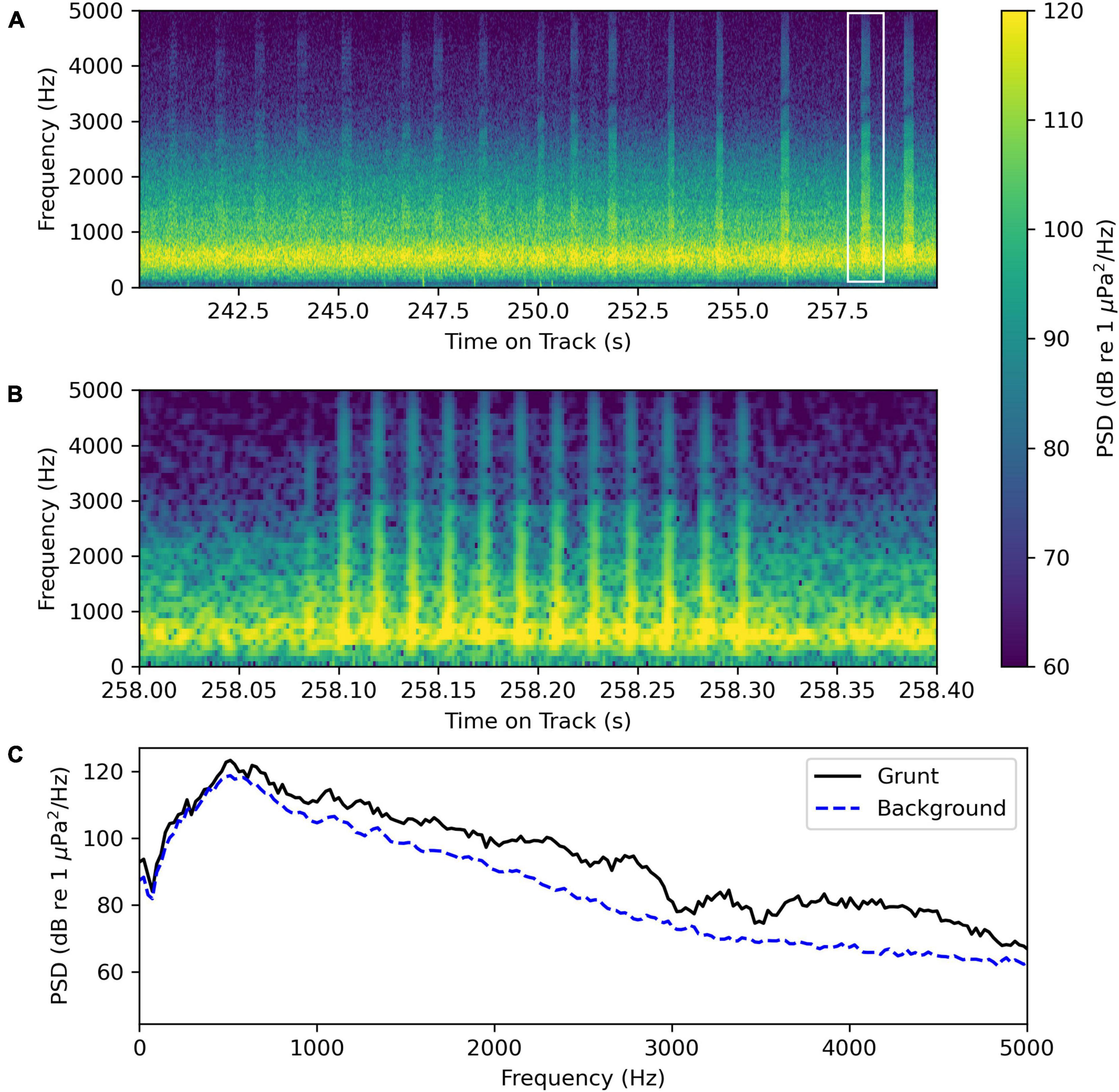
Figure 10. Unknown “grunt” sound recorded by the wave glider Blackbeard at August-01 21:42:31 at latitude and longitude (34.580 348N, 76.635 034W) (Supplementary Sound Clip Audio 3). (A) Spectrogram of a 20 s segment containing s sequence of “grunts.” The in the white rectangle indicates the region on the plot that was analyzed in the next panel (B). (B) Spectrogram of the “grunt” sound in the rectangle in panel (A) using a 512-point FFT for greater time resolution. (C) Average power spectrum of the “grunt” sound shown in panel (B) was taken from 258.05 to 258.35 s and the average power spectrum of the background sound was taken from 256.5 to 257.5 s when no distinct “grunt” was detected. Both average power spectra were computed using 2048-point Hanning windows with an overlap of 1024 points.

Unknown “Buzz” Description

Another sound in the recordings produced by an unknown source is a “buzz” call often detected later in the evening than the unknown “grunt” sound (Figure 11 and Supplementary Sound Clip Audio 4). Figure 11A shows a spectrogram of a recording segment with several unknown “buzz” sounds. Figure 11B shows a spectrogram of an individual “buzz” call, and Figure 11C shows an average power spectrum of the same “buzz” call and the average power spectrum of the background noise taken on an interval when there was no distinct “buzz” call present, but much of the background noise is likely due to other “buzz” calls in the distance. The dominant frequency of the “buzz” call is 1123 Hz with significant energy in frequencies from 400 to 4000 Hz. Examining the oscillogram with an 800–5000 Hz bandpass filter, the buzz consists of 28 pulses with a pulse period of (8.5 ± 0.4)×10⁻³ s and a pulse repetition rate of (118 ± 5) Hz. We detected the loudest unknown “buzz” choruses in the evening after 23:00, but also detected quieter choruses earlier in the evening. The unknown “buzz” chorus can be distinguished from striped cusk-eel choruses that have similar frequency content because the “buzz” calls have many more frequency bands than the striped cusk-eel calls. Also, unknown “buzz” choruses tend to have so many calling fish that the power spectral density and PSB sum values do not vary much over short time scales (60 s to 600 s) as striped cusk-eel choruses do. See the unknown “buzz” and striped cusk-eel choruses identified in Figure 7 for an example of these patterns of time variation.

FIGURE 11

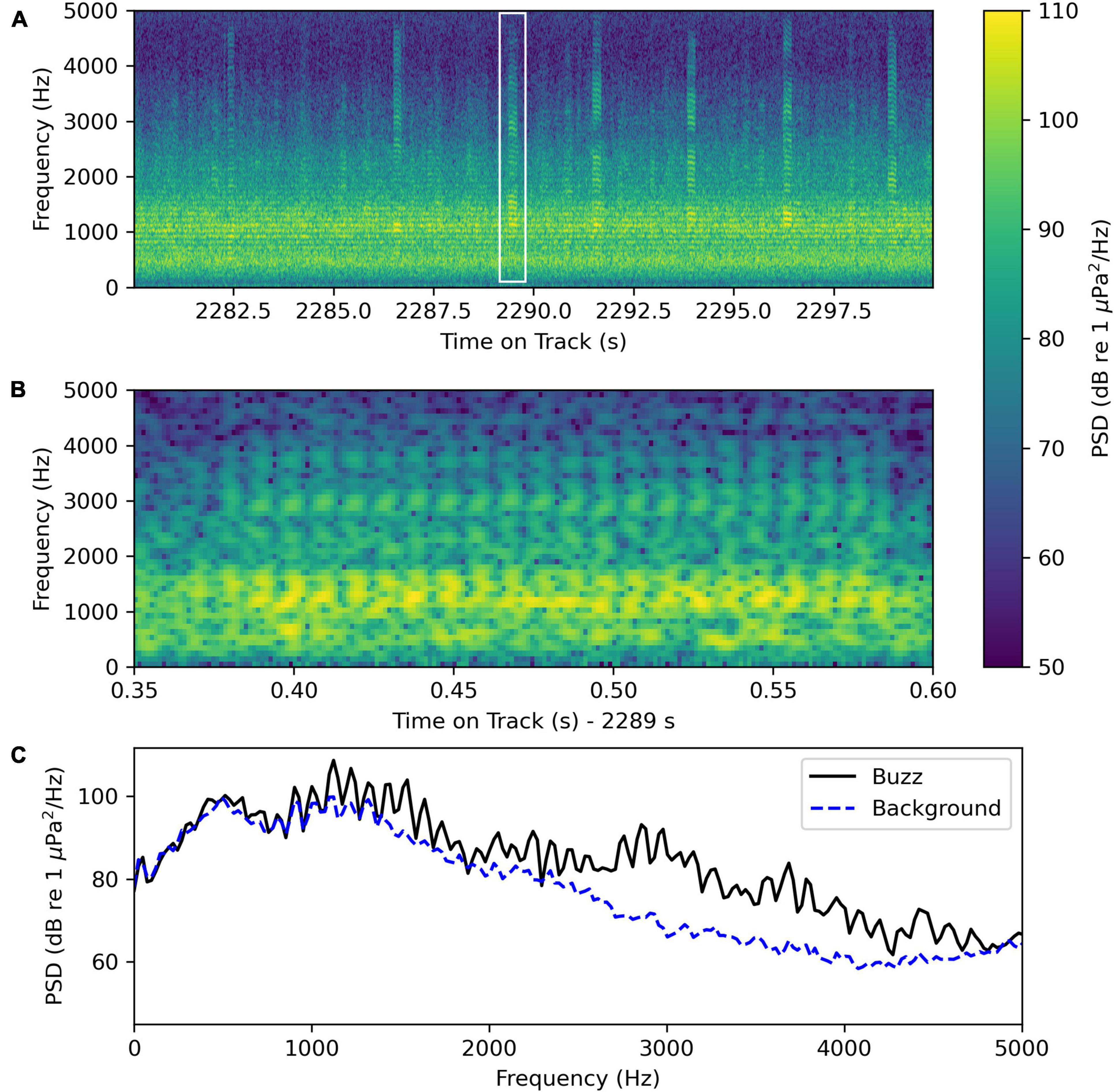
Figure 11. Unknown “buzz” sound recorded by the wave glider Blackbeard at August-02 00:16:23 at latitude and longitude (34.550 280N, 76.649 032W) (Supplementary Sound Clip Audio 4). (A) Spectrogram of a 20 s segment containing several distinct “buzz” calls. The in the white rectangle indicates the region on the plot that was analyzed in the next panel (B). (B) Spectrogram of the “buzz” call in the rectangle in panel (A) using a 512-point FFT for greater time resolution. (C) Average power spectrum of the “buzz” sound shown in panel (B) was taken from 2289.35 to 2289.60 s and the average power spectrum of the background sound was taken from 2289.60 to 2290.00 s when no distinct “buzz” sounds were detected. Both average power spectra were computed using 2048-point Hanning windows with overlaps of 1024 points.

Reef Sound Description

In addition to the fish choruses, the recordings show changes in the 4000–10,000 Hz PSB sum, which is dominated by a 5600 Hz sound that we detected at night in the vicinity of live-bottom reefs. The composite spectrograms in Figures 2B, 4B, 5B, 7B, and 8B each show this reef sound at different levels as the wave glider approached reefs offshore at night. The reef sound was nocturnal and not present in daytime recordings. It is not due to instruments on the glider itself, which we turned on both day and night and turned off at times; the reef sound was independent of the instrument duty cycles. It was not due to the instruments or rudder motor on the wave glider.

Anthropogenic Noises: Sonar and Vessel Noise

We noted a peak in PSB sum in Band I on August-01at 19:36 due to a large cargo vessel nearby (4 km range; see Figure 4 and Supplementary Sound Clip Audio 15). There were numerous vessels recorded during the mission and their location relative to the wave glider was determined from the AIS records broadcast by each vessel and received by the wave glider. The relative position of these known sound sources was computed by mapping the position of the wave glider when vessel noises were recorded on the hydrophone. The maximum received vessel PSB sum value on August-01 was 105.7 dB re 1 μPa² in the PSB Band I 100–200 Hz and 100 dB re 1 μPa² in the Band III 300–600 Hz. The sciaenid chorus exceeded this level in Band III 124 dB re 1 μPa² later that evening at 21:32.

We heard an 800 Hz tonal sound offshore in 27 m on August-02 at 1948. This is similar to sounds produced by moorings with acoustic instruments used to sense ocean currents. Its repetitive tonal sound (2-s pulse in sets of 6 pulses in a narrow band 830 Hz) was distinctive and obvious. It did not overlap in frequency with any biological sounds but it was in the range of biological sounds produced by fish.

Bird Sounds

We detected bird calls that sounded like laughing gulls Leucophaeus atricilla to listeners (Supplementary Figure S10, Sound Clip Audio 13). These birds were heard on August-02 at 19:48. Their calls were an interesting part of the soundscape that was not heard at other times because this was the quietest part of the entire survey. The birds were above the surface when the wave glider was offshore in 27 m deep water. The hydrophone was at a depth of 11 m. Perhaps the birds were following or associated with the surface float of the wave glider. Nonetheless, the fact that they were audible through the air-water interface at this range is impressive. It shows the sensitivity of this passive acoustic system. Presumably, animals underwater can hear birds above the water if they possess similar hearing sensitivity as our hydrophone and recording system.

Comparison With Historical Soundscape Measures

We compared the sound spectra we measured on 2017-August-01 and 2017-August-02 with measurements made by the US Navy researchers in August 1943 to examine any changes over 74 years. Our wave glider passed in the vicinity of Cape Lookout (within 32 km of the approximate location; comparison map shown in Figure 12). We computed frequency band SPLs that matched the octave bands used by the US Navy researchers so that we could compare sound pressure levels in the soundscape in the two studies. The sound pressure level in the band from 1600 to 3200 Hz was 131 dB re 1 μPa in 1943-August-01 at 18:30 at a ship-borne hydrophone station approximately 20 miles south of Cape Lookout NC (Dobrin, 1947), after converting the data in that paper’s Figure 1. The author attributed the source of the sounds to a “croaker” or Sciaenidae fish, but he was not sure which species, suggesting that the “bastard trout,” now called the silver sea trout Cynoscion nothus, was the source. We measured the maximum frequency band fast time constant SPL in that octave band as 136 dB re 1 μPa on 2017-08-01 at 23:32:44 (latitude: 34.558 813 N, longitude: 76.644 667 W). The fish chorusing at the time of our measurements were producing the unknown “buzz” sound. If these sounds were produced by the same two species of Sciaenidae chorusing, the August 2017 measurement was 5 dB higher than in August 1943.

FIGURE 12

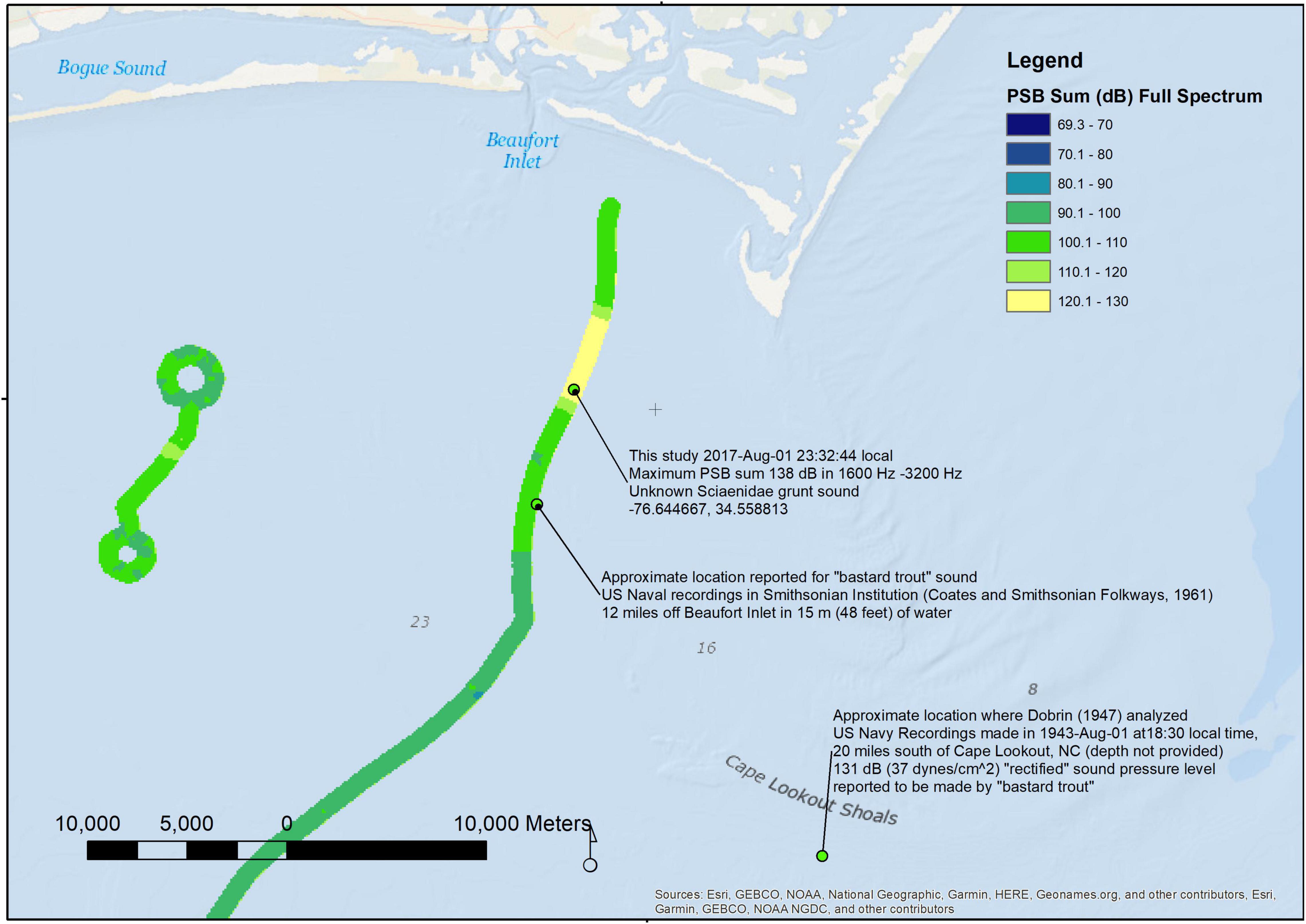
Figure 12. A map of wave glider track August-01 through August-02 2017 near Cape Lookout, NC, United States for comparison with approximate locations of the United States Navy recordings of “bastard trout” analyzed by Dobrin (1947); the full-spectrum PSB sum (dB re 1 μPa²/Hz) has been overlaid on the track.

We compared a second recording in the Sciaenidae frequency range with US Navy measurements reported from 1943 in Figure 1 of Dobrin (1947). The maximum sound pressure level (SPL) during the mixed-species Sciaenidae chorus in August 2017 in this study was 138 dB re 1 μPa in the range 300 to 600 Hz. This was compared with historical levels measured near that location in August 1943 by the US Navy; the chorus we recorded was 25 dB higher (112 dB re 1 μPa in the 200 to 800 Hz range 1943, Dobrin, 1947). This comparison shows a dramatic increase in the SPL associated with Sciaenidae calling and the unknown “grunt” from August 1943 to August 2017.

Map of Fish Choruses

A summary map of the fish chorus and reef sound distribution was produced. A plot of the PSB sums in Bands I, III, V, VI, and VII was produced to delineate the geographic distribution of the fish choruses along our wave glider track, limited to where these sums exceeded the 90th percentile of all sums in each band (Figure 13). This 90th percentile was a threshold chosen to conservatively delimit and plot the linear extent of the fish choruses and reef sounds. Band I (100 to 200 Hz, PSB sum exceeding 112 dB re 1 μPa² indicated by red lines in Figure 13) delimited areas dominated by red drum, grouper growls, and black drum. These choruses occurred both at artificial and natural reefs in water <20 m and offshore in 27 to 30 m, where natural reefs occurred based on the distribution of the reef sounds in Band VII (PSB sums exceeding 106 dB re 1 μPa² indicated by orange lines in Figure 13). Band III (300 to 600 Hz PSB sums exceeding 116 dB re 1 μPa² indicated by blue lines in Figure 13) delimited areas with the Sciaenidae mixed chorus and the unknown “grunt,” which is also likely to be a sciaenid fish. These choruses were limited to areas near Cape Lookout Shoals and New Topsail Inlet but produced the greatest SPL values (142 to 148 dB re 1 μPa) during the survey. Band V (1500 to 2000 Hz PSB sums exceeding 113 dB re 1 μPa² indicated by green lines in Figure 13) was associated with striped cusk-eels. These striped cusk-eel choruses occurred near Cape Lookout Shoals, offshore in 27 to 30 m depth, near New Topsail Inlet, and around both natural and artificial reefs. Finally, the Band VI (1600 to 3200 Hz PSB sums exceeding 114 dB re 1 μPa² indicated by purple lines in Figure 13) delimited the choruses of the species making the unknown “buzz” sound. These were found at Cape Lookout Shoals, offshore in 27 to 30 m depth, at artificial reefs outside New Topsail Inlet, and at both artificial and natural reefs.

FIGURE 13

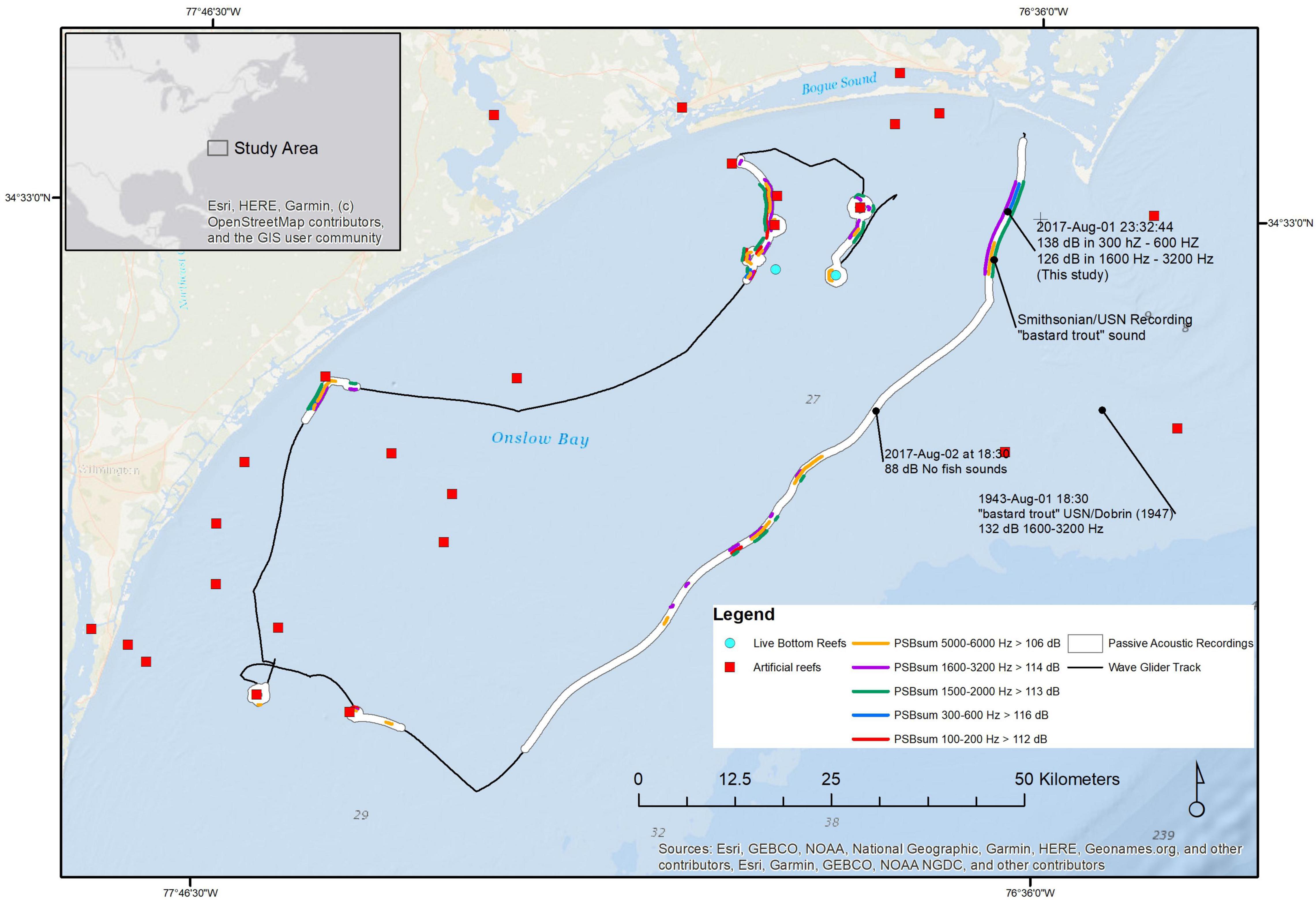
Figure 13. A map of wave glider track (dashed lines; open white circles indicate the position every 4 h, orange filled circles indicate the position at sunset at the time indicated) August-01 through August-09 with the full-spectrum PSD sum (dB re 1 μPa²/Hz) overlaid on the track. Locations along the track where individual species’ calls and mixed-species fish choruses were recorded are labeled. The locations of artificial reefs (red circles; source: North Carolina Division of Marine Fisheries NCDMF) and known natural reefs (aqua circles) are indicated. The position of a cargo ship on August-01 was obtained from vessel Automatic Identification System (AIS) signals received on the wave glider and are shown as blue circles.

Discussion

We introduced this paper with an analogy of the terrestrial soundscape changing while one is driving into the country from the city. In this study, we drove the wave glider towing a hydrophone and passive acoustic recorder from a point just offshore from the busy ship port area of Beaufort Inlet, NC, with its shipping channel frequented by both small vessels and large cargo vessels, along a path that headed offshore into deep, quiet water, traveling southwest near the edge of the Gulf Stream, then returning inshore to glide past artificial and natural reefs. As we made that trip offshore, the soundscape became less noisy (full-spectrum PSB sum declined due to less vessel and less biological noise), and individual animals could be heard calling. We recorded a Sciaenidae chorus, an unknown “grunt” chorus, an unknown “buzz” chorus, and a striped cusk-eel chorus inshore between Beaufort Inlet and Cape Lookout Shoals and another mixed-species chorus near New Topsail Inlet. We could only identify calling species if they were close by and above the background sound levels, typically early in the evening. Recordings made early in the evening were better for fish sound identification. Offshore, we heard individual grouper “growls,” black drum “booms,” silver perch “clucks,” sea robin “honks,” and oyster toadfish “boat whistle” calls in the deeper water. We also heard birds calling from above the surface. We recorded an 830 Hz tone from an unknown source that sounds very much like a low-frequency sonar signal. Finally, we heard reef sounds, rainfall, and thunder in the soundscape. The inshore ocean “city” soundscape transitioned from a cacophony into an offshore “country” soundscape that was quieter, yet quite diverse, and then returned to a louder inshore “city” mixed-species chorus near New Topsail Inlet and artificial reefs composed of Sciaenidae, Ophidiidae, and unknown “grunt” sounds occurring during a rainstorm that reached a maximum SPL of 142 dB re 1 μPa.

A Soundscape Revisited: Atlantic Ocean off North Carolina in World War II

Dobrin (1947), working for the US Navy with recordings made with hydrophones near our survey site, wrote about the soundscape in the Atlantic Ocean that he heard. This provided us with historical comparisons of SPLs. At the time, the Atlantic Ocean off North Carolina was known as “Torpedo Junction” and was a battleground for German submarines, which were sinking United States cargo ships and supply vessels (Hickam, 1996). Anti-submarine efforts using passive sonar was a primary defense strategy for the US Navy, and because underwater noises from biological sources were dominating the soundscape, it was important to characterize the fishes and other marine life causing interference in the detection of ships and submarines (Horton, 1959). Horton wrote: “It is now known that fish noise is the limiting interference to the operation of sonar equipment in many locations” (page 63, Horton, 1959). Thus, the spectrum levels of fish sounds relative to vessel noise was being carefully measured by US Navy researchers. The US Navy wanted to hear enemy submarines and vessel noises, but instead, the hydrophones recorded biological noises every night. Both Dobrin (1947) and Horton (1959) attributed these biological fish sounds to “croakers” and other members of the Sciaenidae. Dobrin had access to recordings from all along the east coast of the United States, but made note of the sound pressures measured “…from a boat in the open Atlantic, approximately 20 miles offshore south of Cape Lookout, NC…” (page 20, Dobrin, 1947) and speculated as to the identity of the source. This US Navy recording was 74 years before our measured PSB sums were computed at approximately the same location. In Dobrin’s Figure 1, the maximum octave band pressure measured in 1943-August-01 at this location for the 1600 to 3200 Hz band was “37 dynes/cm²/$\sqrt{\text{octave}}$,” which is equivalent to an octave band SPL of 131 dB re 1 μPa at this site. Dobrin’s recording system produced mean rectified sound pressures. His value is equivalent to an RMS octave band SPL of 132 dB re 1 μPa. He suggested the identity of the fish producing this sound was the “bastard trout,” now known by its American Fisheries Society common name (Nelson et al., 2004) as the silver seatrout C. nothus. We suspect this species identification was incorrect, and that the US Navy and our wave glider system recorded striped cusk eels O. marginatum in that frequency range. A recording of this sound is still available¹ and can be compared with known captive and field-recorded striped cusk eels sounds (Sprague and Luczkovich, 2001) spectrographically. The sound of the “bastard trout” C. nothus was published as part of a record album and cassette tape, made from US Naval Research hydrophone recordings in the summer of 1943 off Fort Macon, Cape Lookout, and Beaufort, North Carolina (Coates and Smithsonian Folkways, 1961). These are undoubtedly part of the same sound recordings that were used by Dobrin (1947) to compute his measurements of sound pressure levels (both Dobrin and the Smithsonian relied on US Naval hydrophone recordings in coastal waters off Cape Lookout, NC in the summer of 1943, the same area where we surveyed). Other than the general location reported above, where precisely the Dobrin recording was made, and at what depth in the water column the US Navy hydrophone was deployed is unknown [although Horton (1959), as the US Navy’s main sonar expert at this time, was well aware of vessel self-noise causing interference in hull-mounted hydrophones and mentions that “cable-connected buoys” were often used (Horton 199, Chapter 7, “Direct Listening,” pages 303–305)].

Near Cape Lookout, the wave glider measured a loud chorus in the same octave band observed by Dobrin on 2017-August-01, 74 years after the Dobrin recording was made. Our measurements had a peak PSB sum for Band VI (1600 to 3200 Hz) of 126 dB re 1 μPa² at time 23:33. We calculated band-filtered SPLs in the recording for that time and obtained a peak level of 136 dB re 1 μPa using a fast time constant and 132 dB re 1 μPa using a slow time constant. These levels are consistent with Dobrin’s results. The time of day for our peak levels was later in the evening (2017-August-01 at 23:33 vs. 1943-August-01 at 18:30 for Dobrin, 1947). Finally, the sound source of their recording was incorrectly attributed to silver sea trout C. nothus, which sound is now known to be produced by striped cusk eels O. marginatum; we have attributed our peak pressure measurement to the unknown “buzz” sound, although striped cusk eel also contributes to the sound pressure measurement in this frequency range. This fish making our “buzz” sound remains to be identified. Dobrin (1947) was measuring the striped cusk eel “chatter” calls.

On the following day, the wave glider passed over 27 m depth (a similar depth to that approximate position reported by Dobrin) at 18:30 on August-02, but our measured PSB sum levels were much lower, ∼ 80 dB re 1 μPa². This discrepancy in measured sound pressures could be the depth of the hydrophone in each measurement; if Dobrin’s measurement was taken near the bottom, it would have been more intense, since that is where the striped cusk-eels bury; our hydrophone was towed at 11 m depth. We did not hear striped cusk-eels or the unknown grunt at that depth, however. These observations suggest that there has been a decline in the sound contribution of whatever species of fish, striped cusk-eels or an unknown sciaenid fish, made the sounds at that frequency over three-quarters of a century ago. Perhaps these choruses have shifted inshore to shallower water since 1943.

The main contributor to the soundscape in that frequency range is still unknown: it is due to the species that makes the unknown “buzz” sounds, which we will discuss next. Other Sciaenidae identified in the soundscape in the Atlantic Ocean near Morehead City and Cape Lookout included Atlantic croaker, M. undulatus, weakfish, C. regalis, red drum S. ocellatus, and black drum P. cromis. Dobrin (1947) was surprised at the intensity of the sounds produced by these “croakers” and Horton (1959, page 63) later wrote, “fish noise” was “…greeted with some astonishment” by workers in the field of underwater acoustics and was much louder than vessel noise in some spectral bands. Dobrin (1947) reported even higher SPLs during 1942–1943 in the Sciaenidae chorus octave (200 to 800 Hz) at a different site (Wolf Trap in Lower Chesapeake Bay in July 1942), with the maximum SPL of 142.7 dB re 1 μPa. These fish choruses were louder than nearby vessel noise, as Dobrin recognized, and this made enemy vessel detection in this soundscape complicated. Horton (1959) devised a solution to this problem in some cases by using electronic high-pass filters to detect propellor noises in frequency bands above the fish frequencies. But as can be observed in our recordings, vessel noises greatly overlap fish sounds in the frequencies they each produce, and the overlap in frequency results in masking of vessel noise by fish choruses (for those trying to detect vessels), and vessel noises result in false positives (for those relying on PSB sums to detect fish choruses). We conclude that the soundscape of Cape Lookout North Carolina is dominated by Sciaenidae and Ophidiidae fishes and has shifted over 74 years to shallower water, and may be even louder than 74 years ago.

Sciaenidae Fish May Produce the Unknown “Grunt” Chorus

We here hypothesize that the identity of the unknown grunt sound is likely to be banded drum Larimus fasciatus Sciaenidae, based on some work done on the reproductive biology of the banded drum in the area previously (Ross, 1984). A congener Larimus breviceps was recorded (Fish and Mowbray, 1970) that has similar frequency spectra characteristics. These authors recorded disturbance calls in an aquarium, which are not similar to the pulse pattern in our unknown grunt, but disturbance call pulse rates may not be reflective of actual calling rates occurring during reproduction in the wild. Recent soundscape recordings of the fish choruses (their “Chorus I”) from protected reefs in Brazil have been attributed to L. breviceps (Borie et al., 2021) and these calls appear very similar to the unknown grunt sound, based on spectral analyses of the two choruses. The reproductive biology of the banded drum was described by Ross (1984) at a site very close to where we recorded the unknown grunt chorus, near Cape Lookout, NC. In that study, the peak spawning season for banded grunt in North Carolina is August each year (Ross, 1984), the same time of year and nearly the same depths and locations where we recorded our unknown grunt Sciaenidae chorus. We are investigating this hypothesis actively now. Our earlier report that the sciaenid grunt recorded there was produced by spotted sea trout C. nebulosus (Luczkovich et al., 2019), is most likely incorrect, as the frequency of the sound is more similar to L. breviceps than C. nebulosus.

Incorrect Species Identification in Field Settings

Fish and Mowbray (1970) wrote “To identify with precision and certainty sounds monitored in the field without seeing the organism that produced them is considered impossible by many investigators; such identification must be considered circumstantial at best (page xiv).” This is still an issue, despite the efforts by these authors, Dobrin (1947) and many others to establish a reference library of fish sounds. Dobrin (1947) also recognized the issue and successfully added multiple known species calls to the list by recording sounds from fishes in captivity. Nonetheless, both studies incorrectly identified the sounds produced by the striped cusk-eels as being produced by members of the Sciaenidae: in Dobrin (1947) the bastard trout, silver seatrout C. nothus, and in Fish and Mowbray the weakfish C. regalis. This misidentification was later corrected by the current authors (Sprague and Luczkovich, 2001). However, we have also committed a misidentification in the first publication from the wave glider survey discussed above, attributing the unknown grunt sound to spotted sea trout C. nebulous (Luczkovich et al., 2019). We have two unknown sounds (the “unknown grunt” and the “unknown buzz”) in the current survey and we are choosing here not to definitively identify these. Rather, we propose additional captive fish recording studies to identify potential sound-producing species in the area when this survey was done to identify the sound sources, as has been recommended by several authors (Riera et al., 2017; Rountree and Juanes, 2020). This is not an easy exercise and takes a dedicated team of fish bioacoustics experts and fish biologists with the proper equipment and experimental tanks, or other fish-holding facilities like net pens in the open sea to separate species and get them to make the same calls in captivity, preferably in a setting with no tank walls (free-field) (Aalbers and Drawbridge, 2008). The matching of species to sounds produced in the field might also be accomplished with underwater video and ROVs equipped with calibrated hydrophones (Sprague and Luczkovich, 2004). Until such studies are accomplished with the Cynoscion and Larimus species in the Sciaenidae and other species in the families Triglidae, Batrachoididae, and Ophiididae listed above, we cannot determine the species producing the unknown sounds recorded in the choruses reported here with any degree of certainty.

Sciaenidae Fish Choruses Dominate Ocean Soundscapes

Sciaenidae fishes are known to produce loud choruses around the world, as we have shown here. The loudest fish chorus reported to date was in the Gulf of California by Gulf corbina Cynoscion othonopterus (Erisman and Rowell, 2017). The RMS sound pressure level of the Gulf corbina chorus was measured with a calibrated hydrophone system as 166.6 dB re 1 μPa, with individual fish pulses reaching 190 dB re 1 μPa. In China’s Pearl River estuary, the sciaenid species Belanger’s croaker Johnius berlangerii, big-snout croaker J. macrorhynus, and the lionhead Collichthys lucida produce nocturnal choruses that report a mean received levels of 140.5 dB re 1 μPa (Pine et al., 2017). Near the mouth of the May River, South Carolina (United States), spotted seatrout C. nebulosus were recorded as having a chorus with a power spectral density of 120 dB re 1 μPa²/Hz at 239 Hz, and other Sciaenidae (silver perch B. chrysoura 110 dB at 1133 Hz, black drum P. cromis 90 dB at 82 Hz, red drum S. ocellatus 110 dB at 144 Hz) were recorded (Monczak et al., 2017). Red drum have been recorded in North Carolina estuaries at an RMS sound pressure of 130 dB re 1 μPa during the same season as reported here (August–October; Luczkovich unpublished), but this study shows that they produce sounds offshore in the Atlantic Ocean off of North Carolina. Red drum have been previously reported to occur and produce mating sounds in estuaries (Luczkovich et al., 1999a; Lowerre-Barbieri et al., 2008; Montie et al., 2016) as well as offshore in the Gulf of Mexico (Holt, 2008). In kelp forests of the Pacific Ocean, white seabass Atractoscion nobilis (Sciaenidae) mate in the ocean forming large chorus-producing aggregations of multiple males (up to nine males) and a single female; the males’ sounds were described as “pulses trains” (81 Hz peak frequency), “drumrolls” (77 Hz), “thuds” (70 Hz), “booms” (63 Hz), and “chants,” the latter of which consisted of “drum rolls” and “thuds” produced together in succession (Aalbers and Drawbridge, 2008). These various call types were associated with observed spawning behavior and gamete releases. Unfortunately, only relative SPL was reported by the authors, so we cannot compare the SPLs with other Scianeidae choruses, but these authors reported relative SPL dB values for each sound type that suggested they were quite loud. Because these authors were able to observe spawning behavior in association with hydrophone recordings in an open-ocean pen with multiple individual white sea bass, a great deal more was learned about the sound use in attracting mates than in a typical study of passive acoustic recorded fish sounds. One possible study may have measured the white seabass “chanting” chorus sound pressure levels. A wave glider with a calibrated passive acoustic recorder attached, mentioned earlier, apparently recorded these white seabass choruses in kelp forests off California, and the received levels for the unidentified chorus in 60 to 300 Hz range (their “Chorus Type III”) peaked at 125 dB re 1 μPa (Pagniello et al., 2019). One can speculate that this was the received levels of white sea bass “chants,” i.e., a chorus of white seabass spawning near or in a kelp forest. Atlantic croakers have the same spawning season (August–October) but are now also confirmed to call offshore during this time. These two Sciaenidae species have already been reported as spawning both in the estuary and offshore, although not based on passive acoustics.

Black drum have been reported to occur further offshore in deep water in Onslow Bay using fixed passive acoustic recorders, but they were most commonly heard in the spring (Rice et al., 2016). We found black drum inshore near estuary inlets and artificial reefs in Onslow Bay in the late summer (August). It is now apparent that black drum may move from offshore to inshore regions and do not reside in one place all year. It is also apparent that they make sounds in the non-breeding period. Black drum are reported to spawn, based on passive acoustics of the spawning call from Jan through April (Locascio et al., 2012; Rice et al., 2016, 2017). The sounds we recorded suggest a different extended spawning period in North Carolina or the sounds are also produced by non-spawners. This bears further investigation.

The Identification of Habitat (Depth Zones, Temperature, Bottom Type, Currents)

For Sciaenidae like red drum, black drum, Atlantic croaker, and the unknown Sciaenidae “grunt” producer, their habitat used extends outside of estuaries. We can now place some seasonally varying depth boundaries using mobile passive acoustic surveys. because the wave glider can measure currents with the ADCP, we can examine patterns of spawning habitats in currents of different magnitude.

We can locate an acoustic reef signature, so reef habitats can be mapped in this way. We suspect that the reef sound is a product of multiple reef-associated species, including snapping shrimp in the family Alpheidae (Lillis and Mooney, 2018).

Fixed vs. Mobile Passive Acoustic Surveys

Mobile passive acoustic surveys allow maps of soundscapes and marine animal behavior to be produced over a wide area (Wall et al., 2012; Luczkovich et al., 2019; Pagniello et al., 2019); while fixed passive acoustic recorders measure the soundscape around points in space. The spatial coverage of soundscape studies with mobile passive acoustics recorders is large, but temporal coverage of any given location is short; in contrast, temporal coverage of a fixed recorder is long, but the spatial coverage is small. However, this presents challenges in survey design, especially when sound sources vary greatly diurnally, as is common in biological sources like fish choruses. Because the spatial coverage provided by mobile passive acoustic systems does not allow for temporal persistence at a given point, incomplete diurnal coverage will occur across the survey. Care must be taken in survey design to sample similar areas at similar times of the day to make meaningful comparisons. This became apparent in our circular paths around artificial and natural live bottom reefs, which were not completed at the same time of the night for each reef type, and peak fish chorusing occurred at times when the wave glider was transiting between the artificial and natural reefs. Nocturnal calling behavior means that mobile passive acoustic surveys cannot map areas transited during the daytime, but a sampling scheme could be devised where daytime gaps in the recording surveys are revisited at night on subsequent days. This sampling design could work to correct this problem.

Nonetheless, survey work using a passive acoustic equipped wav glider can be accomplished with minimal disturbance to the animal’s behavior, as the wave glider makes very little noise. An important consideration for any mobile hydrophone is the self-noise of any vessel that deploys or tows the hydrophone. We believe our system, with a tow body and an alternating float and sinker cable connecting the tow body to the submarine (Figure 1), which was designed to acoustically isolate the passive acoustic recording system (Saint Andrews Instrumentation Laboratory, 2015), provided us with the greatest signal-to-noise ratio one can expect to achieve with a mobile system. We had a hydrophone operating with great sensitivity in mid-water depths (8 to 11 m below the surface), away from surface wave noise. Although the hydrophone in the towbody varied in sampling depth due to changes in the wave glider speed over ground and currents, it was not always at a constant water depth (mean 9.6 m). Although not done in this study, in the future, because tow body depth was monitored throughout the survey using a depth pressure sensor, this depth variation could be addressed computationally by adjusting the received sound levels for variation in tow body depth. Buoyancy gliders (Slocum gliders) have been used as passive acoustic monitoring systems (Wall et al., 2012), but vary with depth by design The relative depth stability of the wave glider passive acoustic system is regarded here as an advantage for soundscape studies over a buoyancy glider mounted hydrophone system. Because the tow body was pulled 15 m behind the wave glider submarine, this design limited interference from the SV2 wave glider float and submarine noise. In addition, there was no propellor noise on the Liquid Robotics SV2, unlike the submarine-mounted hydrophone used with an SV3 (Pagniello et al., 2019). The wave glider itself is relatively quiet (Wiggins et al., 2010). The combination of the high-sensitivity hydrophone in a tethered acoustically isolated tow body towed at a relatively constant depth provided a low-noise, low-interference platform, and a high signal-to-noise ratio.

In the future, we would recommend that PSB sums for Sciaenidae and other species in the frequency bands listed in Table 2 be processed on the Decimus board and provided in real-time via reports in the Wave Glider Management System (WGMS). This PSB sum summary would then be useful for shore operators to direct the wave glider while at sea to adaptively sample for fish calls based on real-time reports via WGMS; fish choruses could be better mapped for habitat use and spawning behavior.

Conclusion

We surveyed the offshore Atlantic Ocean soundscape using passive acoustic systems on a wave glider which allowed us to survey persistently and unobtrusively along a pre-planned route moving from inshore areas near inlets with loud choruses by mixed-species of Sciaenidae fishes to quieter areas offshore on live reefs with groupers, toadfish, black drum, and sea robins. The passive acoustic system we recorded with had a very sensitive recording level and wide dynamic range and was unaffected by the wave glider propulsion (no propellor sounds, tow cable strumming, and no instrument self-noise). Based on previous fish sounds associated with species recorded in controlled conditions, we identified five species of Sciaenidae fishes chorusing in the offshore areas near Beaufort Inlet and New Topsail Inlet in North Carolina (United States) including weakfish C. regalis, Atlantic croaker M. undulatus, red drum S. ocellatus, and black drum P. cromis.

There were some previously unknown fish sounds. We described the “grunt” sounds of an unknown Sciaenidae species likely to be banded drum, L. fasciatus, but we cannot eliminate also be the silver seatrout, C. nothus, as speculated by Dobrin (1947). However, we did discover that the recording purported to be C. nothus by Dobrin and published by the Smithsonian based on US Naval research recordings (Coates and Smithsonian Folkways, 1961), is a misidentification and was made by striped cusk eels, O. marginatum.

Finally, we compared the two sets of fish chorusing recordings and SPL measurements that were made 74 years apart and showed an increase in SPL. This comparison may be a change in fish spatial distribution, with the chorusing fish moving into shallower water in 2017. Nonetheless, the fish chorusing we recorded was higher than in the US Navy recordings made at Cape Lookout in August 1943.

Data Availability Statement

The datasets presented in this study can be found in online repository. The URL for the data is https://dataverse.unc.edu/dataverse/GliderSoundscape2021.

Author Contributions

Both authors planned the study, organized all the data collections and recordings, wrote the manuscript together, and collaborated in spectral analysis and data interpretation.

Funding

This work was supported by National Science Foundation Major Research Instrumentation Grant “MRI: Acquisition of an Acoustic Wave Glider” (Grant No. 1429315) to the co-authors, Roger A. Rulifson and John P. Walsh of East Carolina University. We also received matching funding from the East Carolina University Division of Research and Economic Development (REDE), The Thomas Harriot College of Arts and Sciences, The Institute for Coastal and Science and Policy (ICSP), and The Department of Biology, and the Department of Physics at East Carolina University.

Conflict of Interest

The authors declare that the research was conducted in the absence of any commercial or financial relationships that could be construed as a potential conflict of interest.

Publisher’s Note

All claims expressed in this article are solely those of the authors and do not necessarily represent those of their affiliated organizations, or those of the publisher, the editors and the reviewers. Any product that may be evaluated in this article, or claim that may be made by its manufacturer, is not guaranteed or endorsed by the publisher.

Acknowledgments

We thank the ECU Wave Glider Pilots: Rebecca Asch, Phillip DeVille, Patrick Harris, Tyler Peacock, Roger Rulifson, Chris Thaxton, Jordan Smith, Ryan McKenzie, and the two co-authors. Eric Diaddorio was the vessel captain during launch and recovery and his assistance was much valued. We thank Graham Weatherup and Richard Baggaley of Saint Andrews Instrument Laboratory, Scotland, United Kingdom for assistance with the tow body buoyancy adjustments and Decimus passive acoustic recorder. We also thank Ryan Carlon and Ben Harmon of Liquid Robotics, Inc. for technical support with the SV2 wave glider, Blackbeard.

Supplementary Material

The Supplementary Material for this article can be found online at: https://www.frontiersin.org/articles/10.3389/fmars.2022.779540/full#supplementary-material

Footnotes

1. ^ https://folkways.si.edu/sounds-of-the-sea-vol-1-underwater-sounds-of-biological-origin/album/smithsonian

References

Aalbers, S. A., and Drawbridge, M. A. (2008). White Seabass Spawning Behavior and Sound Production; White Seabass Spawning Behavior and Sound Production. Trans. Am. Fish. Soc. 137, 542–550. doi: 10.1577/T04-058.1

CrossRef Full Text | Google Scholar

Bertucci, F., Lecchini, D., Greeven, C., Brooker, R. M., Minier, L., Cordonnier, S., et al. (2021). Changes to an urban marina soundscape associated with COVID-19 lockdown in Guadeloupe. Environ. Pollut. 289:117898. doi: 10.1016/j.envpol.2021.117898

PubMed Abstract | CrossRef Full Text | Google Scholar

Borie, A., Rezende, S. M., Ferreira, B. P., Maida, M., Radford, C., and Travassos, P. (2021). Soundscape of protected and unprotected tropical atlantic coastal coral reefs. Sci. Mar. 85, 5–14. doi: 10.3989/scimar.05052.001

PubMed Abstract | CrossRef Full Text | Google Scholar

Center for Conservation Bioacoustics (2019). Raven Pro: Interactive Sound Analysis Software (Version 1.6.1). Ithaca, NY: The Cornell Lab of Ornithology.

Google Scholar

Coates, C. W., and Smithsonian Folkways. (1961). Sounds of the Sea: Sonic Fish Sounds. Folkways Records, Album No. FX 6121. Available Online at: https://folkways.si.edu/sounds-of-the-sea-vol-1-underwater-sounds-of-biological-origin/album/smithsonian [accessed Aug 18, 2021].

Google Scholar

Connaughton, M. A. (2004). Sound generation in the searobin (Prionotus carolinus), a fish with alternate sonic muscle contraction. J. Exp. Biol. 207, 1643–1654. doi: 10.1242/jeb.00928

PubMed Abstract | CrossRef Full Text | Google Scholar

Connaughton, M. A., and Taylor, M. H. (2011). Drumming, Courtship, and Spawning Behavior in Captive Weakfish, Cynoscion regalis. Am. Soc. Ichthyol. Herpetol. 1996, 195–199.

Google Scholar

Dobrin, M. B. (1947). Measurements of Underwater Noise Produced by Marine Life. Science 105, 19–23 doi: 10.1126/science.105.2714.19

PubMed Abstract | CrossRef Full Text | Google Scholar

Duarte, C. M., Chapuis, L., Collin, S. P., Costa, D. P., Devassy, R. P., Eguiluz, V. M., et al. (2021). The soundscape of the Anthropocene ocean. Science 371:eaba4658. doi: 10.1126/science.aba4658

PubMed Abstract | CrossRef Full Text | Google Scholar

Erisman, B. E., and Rowell, T. J. (2017). A sound worth saving: acoustic characteristics of a massive fish spawning aggregation. Biol. Lett. 13:20170656. doi: 10.1098/rsbl.2017.0656

PubMed Abstract | CrossRef Full Text | Google Scholar

Fine, M. L., and Lenhardt, M. L. (1983). Shallow-water propagation of the toadfish mating call. Comp. Biochem. Physiol. A Physiol. 76, 225–231. doi: 10.1016/0300-9629(83)90319-5

CrossRef Full Text | Google Scholar

Fish, M. P., and Mowbray, W. H. (1970). Sounds of Western North Atlantic Fishes; a Reference File of Biological Underwater Sounds. Baltimore: Johns Hopkins University Press.

Google Scholar

Gray, G. A., and Winn, H. E. (1961). Reproductive ecology and sound production of the toadfish, Opsanus tau. Ecology 42, 274–282. doi: 10.2307/1932079

CrossRef Full Text | Google Scholar

Greene, C. H., Meyer-Gutbrod, E. L., McGarry, L. P., Hufnagle, L. C., Chu, D., McClatchie, S., et al. (2014). A wave glider approach to fisheries acoustics: transforming how we monitor the n ation’s commercial fisheries in the 21st century. Oceanography 27, 168–174.

Google Scholar

Hickam, H. H. (1996). Torpedo Junction: U-Boat War Off America’s East Coast, 1942. Annapolis: Naval Institute Press.

Google Scholar

Holt, S. A. (2008). Distribution of Red Drum Spawning Sites Identified by a Towed Hydrophone Array. Trans. Am. Fish. Soc. 137, 551–561. doi: 10.1577/t03-209.1

CrossRef Full Text | Google Scholar

Horton, J. W. (1959). Fundamentals of SONAR. Connecticut: United States Naval Institute.

Google Scholar

Kaatz, I. M. (2002). Multiple sound-producing mechanisms in teleost fishes and hypotheses regarding their behavioural significance. Bioacoustics 12, 230–233. doi: 10.1080/09524622.2002.9753705

CrossRef Full Text | Google Scholar

Kaatz, I. M., Rice, A. N., and Lobel, P. S. (2017). How Fishes Use Sound: Quiet to Loud and Simple to Complex Signaling. Amsterdam: Elsevier Ltd, doi: 10.1016/b978-0-12-809633-8.03083-1

CrossRef Full Text | Google Scholar

Lillis, A., and Mooney, T. A. (2018). Snapping shrimp sound production patterns on Caribbean coral reefs: relationships with celestial cycles and environmental variables. Coral Reefs 37, 597–607. doi: 10.1007/s00338-018-1684-z

CrossRef Full Text | Google Scholar

Locascio, J. V., Burghart, S., and Mann, D. A. (2012). Quantitative and temporal relationships of egg production and sound production by black drum Pogonias cromis. J. Fish Biol. 81, 1175-91. doi: 10.1111/j.1095-8649.2012.03376.x

PubMed Abstract | CrossRef Full Text | Google Scholar

Locascio, J. V., and Mann, D. A. (2008). Diel Periodicity of Fish Sound Production in Charlotte Harbor, Florida; Diel Periodicity of Fish Sound Production in Charlotte Harbor. Florida 116:2640. doi: 10.1577/T06-069.1

CrossRef Full Text | Google Scholar

Locascio, J. V., and Mann, D. A. (2011). Localization and source level estimates of black drum (Pogonias cromis) calls. J. Acoust. Soc. Am. 130:1868–79. doi: 10.1121/1.3621514

CrossRef Full Text | Google Scholar

Lowerre-Barbieri, S. K., Barbieri, L. R., Flanders, J. R., Woodward, A. G., Cotton, C. F., and Knowlton, M. K. (2008). Use of Passive Acoustics to Determine Red Drum Spawning in Georgia Waters. Trans. Am. Fish. Soc. 137:562–575. doi: 10.1577/T04-226.1

CrossRef Full Text | Google Scholar

Luczkovich, J. J., Daniel, H. J. III, Sprague, M. W., Johnson, S. E., Pullinger, R. C., Jenkins, T., et al. (1999a). Characterization of Critical Spawning Habitats of Weakfish, Spotted Seatrout and Red Drum in Pamlico Sound Using Hydrophone Surveys, North Carolina Department of Environment and Natural Resources, Division of Marine Fisheries Technical Report F-62. Available Online at: http://hdl.handle.net/10342/7109 (accessed January 20, 2022).

Google Scholar

Luczkovich, J. J., Sprague, M. W., Johnson, S. E., and Pullinger, R. C. (1999b). Delimiting spawning areas of weakfish cynoscion regalis (family sciaenidae) in pamlico sound, north carolina using passive hydroacoustic surveys. Bioacoustics 10, 143–160. doi: 10.1080/09524622.1999.9753427

CrossRef Full Text | Google Scholar

Luczkovich, J. J., Mann, D. A., and Rountree, R. A. (2008a). Passive acoustics as a tool in fisheries science. Trans. Am. Fish. Soc. 137, 533–541. doi: 10.1577/T06-258.1

CrossRef Full Text | Google Scholar

Luczkovich, J. J., Pullinger, R. C., Johnson, S. E., and Sprague, M. W. (2008b). Identifying Sciaenid Critical Spawning Habitats by the Use of Passive Acoustics. Trans. Am. Fish. Soc. 137, 576–605. doi: 10.1577/T05-290.1

CrossRef Full Text | Google Scholar

Luczkovich, J. J., Rulifson, R. A., and Sprague, M. W. (2019). Listening to Ocean Life: monitoring Fish, Marine Mammal Sounds with Wave Glider. Sea Technol. 2019, 16–20.

Google Scholar

Luczkovich, J. J., Sprague, M. W., and Krahforst, C. S. (2011). Hearing and Lateral Line | Acoustic Behavior. Encyclopedia Fish Physiol. 2011, 311–320. doi: 10.1016/B978-0-12-374553-8.00011-3

CrossRef Full Text | Google Scholar

McWilliam, J. N., McCauley, R. D., Erbe, C., and Parsons, M. J. G. (2017). Patterns of biophonic periodicity on coral reefs in the Great Barrier Reef. Sci. Rep. 7:17459. doi: 10.1038/s41598-017-15838-z

PubMed Abstract | CrossRef Full Text | Google Scholar

McWilliam, J. N., McCauley, R. D., Erbe, C., and Parsons, M. J. G. (2018). Soundscape diversity in the Great Barrier Reef: Lizard Island, a case study. Bioacoustics 27, 295–311. doi: 10.1080/09524622.2017.1344930

CrossRef Full Text | Google Scholar

Mok, H. K., and Gilmore, R. G. (1983). Analysis of sound production in estuarine aggregations of Pogonias cromis, Bairdiella chrysoura, and cynoscion nebulosus (Sciaenidae) [Florida]. Bull. Inst. Zool. Acad. Sin. V 22, 157–186.

Google Scholar

Monczak, A., Berry, A., Kehrer, C., and Montie, E. W. (2017). Long-term acoustic monitoring of fish calling provides baseline estimates of reproductive timelines in the May River estuary, southeastern USA. Mar. Ecol. Prog. Ser. 581, 1–19. doi: 10.3354/meps12322

CrossRef Full Text | Google Scholar

Montie, E. W., Hoover, M., Kehrer, C., Yost, J., Brenkert, K., O’Donnell, T., et al. (2017). Acoustic monitoring indicates a correlation between calling and spawning in captive spotted seatrout (Cynoscion nebulosus). PeerJ 5:e2994. doi: 10.7717/peerj.2944

PubMed Abstract | CrossRef Full Text | Google Scholar

Montie, E. W., Kehrer, C., Yost, J., Brenkert, K., O’Donnell, T., and Denson, M. R. (2016). Long-term monitoring of captive red drum Sciaenops ocellatus reveals that calling incidence and structure correlate with egg deposition. J. Fish Biol. 88, 1776–95. doi: 10.1111/jfb.12938

PubMed Abstract | CrossRef Full Text | Google Scholar

Nelson, J. S., Crossman, E. J., Espinosa-Perez, H., Findley, L. T., Gilbert, R., Lea, R. N., et al. (2004). Common and Scientific Names of Fishes from the United States and Canada. Bethesda: American Fisheries Society.

Google Scholar

Nelson, M. D., Koenig, C. C., Coleman, F. C., and Mann, D. A. (2011). Sound production of red grouper epinephelus morio on the west Florida shelf. Aquat. Biol. 12, 97–108. doi: 10.3354/ab00325

CrossRef Full Text | Google Scholar

Nystuen, J. A. (1986). Rainfall measurements using underwater ambient noise. J. Acoust. Soc. Am. 79, 972–982. doi: 10.1121/1.393695

CrossRef Full Text | Google Scholar

Nystuen, J. A., McGlothin, C. C., and Cook, M. S. (1993). The underwater sound generated by heavy rainfall. J. Acoust. Soc. Am. 93, 3169–3177. doi: 10.1121/1.405701

CrossRef Full Text | Google Scholar

Pagniello, C. M. L. S., Cimino, M. A., and Terrill, E. (2019). Mapping fish chorus distributions in southern california using an autonomous wave glider. Front. Mar. Sci. 6:526. doi: 10.3389/fmars.2019.00526

CrossRef Full Text | Google Scholar

Pijanowski, B. C., Villanueva-Rivera, L. J., Dumyahn, S. L., Farina, A., Krause, B. L., Napoletano, B. M., et al. (2011). Soundscape ecology: the science of sound in the landscape. BioScience 61, 203–216. doi: 10.1525/bio.2011.61.3.6

CrossRef Full Text | Google Scholar

Pine, M. K., Wang, K., and Wang, D. (2017). Fine-scale habitat use in Indo-Pacific humpback dolphins, Sousa chinensis, may be more influenced by fish rather than vessels in the Pearl River Estuary, China. Mar. Mamm. Sci. 33, 291–312. doi: 10.1111/mms.12366

CrossRef Full Text | Google Scholar

Press, W. H., Vetterling, W. T., and Teukolsky, S. (2007). Numerical Recipes: The Art of Scientific Computing, Cambridge, UK: Cambridge University Press, 640–719.

Google Scholar

R Core Team (2021). R: A Language and Environment for Statistical Computing. Available Online at: http://www.r-project.org/ (accessed September 1, 2021).

Google Scholar

Rice, A. N., Morano, J. L., Hodge, K. B., and Muirhead, C. A. (2016). Spatial and temporal patterns of toadfish and black drum chorusing activity in the South Atlantic Bight. Environ. Biol. Fish. 99, 705–716. doi: 10.1007/s10641-016-0511-z

CrossRef Full Text | Google Scholar

Rice, A. N., Soldevilla, M. S., and Quinlan, J. A. (2017). Nocturnal patterns in fsh chorusing off the coasts of Georgia and eastern Florida. Bull. Mar. Sci. 93, 455–474. doi: 10.5343/bms.2016.1043

PubMed Abstract | CrossRef Full Text | Google Scholar

Riera, A., Rountree, R. A., and Juanes, F. (2017). Auditioning fish for sound production in captivity to contribute to a catalogue of known fish sounds to inform regional passive acoustic studies. J. Acoust. Soc. Am. 141:3862. doi: 10.1121/1.4988628

CrossRef Full Text | Google Scholar

Ross, S. W. (1984). Reproduction Of The Banded Drum, Larimus fasciatus, In North Carolina. Fish. Bull. 82, 227–235.

Google Scholar

Rountree, R. A., Gilmore, R. G., Goudey, C. A., Hawkins, A. D., Luczkovich, J. J., and Mann, D. A. (2006). Listening to fish: applications of passive acoustics to fisheries science. Fisheries 31, 433–446. doi: 10.1577/1548-8446200631[433:LTF]2.0.CO;2

CrossRef Full Text | Google Scholar

Rountree, R. A., Goudey, C. A., Hawkins, A. D., Luczkovich, J. J., and Mann, D. A. (2003). Listening to Fish: Passive Acoustic Applications in Marine Fisheries. Cambridge: Massachusetts Institute of Technology.

Google Scholar

Rountree, R. A., and Juanes, F. (2020). Potential for use of passive acoustic monitoring of piranhas in the Pacaya–Samiria National Reserve in Peru. Freshw. Biol. 65, 55–65. doi: 10.1111/fwb.13185

CrossRef Full Text | Google Scholar

Saint Andrews Instrumentation Laboratory (2015). Wave Gilder Sv2 Decimus Pam User Guide. Available Online at: http://www.sa-instrumentation.com/ (accessed September 1, 2021).

Google Scholar

Saucier, M. H., and Baltz, D. M. (1993). Spawning site selection by spotted seatrout, Cynoscion nebulosus, and black drum, Pogonias cromis, in Louisiana. Environ. Biol. Fish. 36, 257–272. doi: 10.1007/BF00001722

CrossRef Full Text | Google Scholar

Sprague, M. W., and Luczkovich, J. J. (2001). Do striped cusk-eels Ophidion marginatum (Ophidiidae) produce the “chatter” sound attributed to weakfish Cynoscion regalis (Sciaenidae)? Copeia 2001, 854–859. doi: 10.1643/0045-85112001001[0854:DSCEOM]2.0.CO;2

CrossRef Full Text | Google Scholar

Sprague, M. W., and Luczkovich, J. J. (2004). Measurement of an individual silver perch Bairdiella chrysoura sound pressure level in a field recording. J. Acoust. Soc. Am. 116:3186. doi: 10.1121/1.1802651

CrossRef Full Text | Google Scholar

Sprague, M. W., Luczkovich, J. J., Pullinger, R. C., Johnson, S. E., Jenkins, T., and Daniel, H. J. III (2000). Using spectral analysis to identify drumming sounds of some North Carolina fishes in the family Sciaenidae. J. Elisha Mitchell Sci. Soc. 116, 124–145.

Google Scholar

Tellechea, J. S., Fine, M. L., and Norbis, W. (2017). Passive acoustic monitoring, development of disturbance calls and differentiation of disturbance and advertisement calls in the Argentine croaker Umbrina canosai (Sciaenidae). J. Fish Biol. 90, 1631–1643. doi: 10.1111/jfb.13257

PubMed Abstract | CrossRef Full Text | Google Scholar

Vieira, M., Fonseca, P. J., and Amorim, M. C. P. (2021). Fish sounds and boat noise are prominent soundscape contributors in an urban European estuary. Mar. Pollut. Bull. 172:112845. doi: 10.1016/j.marpolbul.2021.112845

PubMed Abstract | CrossRef Full Text | Google Scholar

Wall, C. C., Lembke, C., and Mann, D. A. (2012). Shelf-scale mapping of sound production by fishes in the eastern Gulf of Mexico, using autonomous glider technology. Mar. Ecol. Prog. Ser. 449, 55–64. doi: 10.3354/meps09549

CrossRef Full Text | Google Scholar

Wiggins, S., Manley, J., Brager, E., and Woolhiser, B. (2010). Monitoring marine mammal acoustics using wave glider. MTS/IEEE Seattle Oceans 2010, 8–11. doi: 10.1109/OCEANS.2010.5664537

CrossRef Full Text | Google Scholar