Abstract
The ecological characteristics of mesopelagic community are crucial to understand the pelagic food web, replenishment of pelagic fishery resources, and building models of the biological pump. The deep scattering layers (DSLs) and diel vertical migration (DVM) are typical characteristics of mesopelagic communities, which have been widely observed in global oceans. There is a strong longitudinal environmental gradient across the tropical Pacific Ocean. Nevertheless, the longitudinal variation of DSLs along this gradient was still largely unclear until now. We investigated the DSLs across the tropical Pacific Ocean using data of shipboard acoustic Doppler current profiler at 38 kHz from July to December 2019. The study area was divided into three sub-regions by cluster analysis of environmental variables: the western part (WP), the transition part (TP), and the eastern part (EP). The result confirmed that the longitudinal variation of DSLs and DVM: the weight migrating depth of mesopelagic organisms was reduced from 571.2 ± 85.5 m in the WP to 422.6 ± 80.8 m in the EP; while the migrating proportion was minimum in the TP (35.2 ± 12.8%), and increased to 86.7 ± 16.2% in the EP. Multiple regressions analysis showed that both the mesopelagic average oxygen and chlorophyll a concentration were significant factors which influenced the upper boundary depth and weight migrating depth, while the center mass depth was only influenced by the chlorophyll a. Since higher demand of most predators of mesopelagic animals for dissolved oxygen and light intensity, the limitations of predator behavior by environmental conditions might explain the observed spatial heterogeneity of DSLs. Combining the previous results and the findings of this study, it implied that declined biomass, shallower habituating depths, and lower migration proportion of mesopelagic animals under more extremely oligotrophic conditions with global change in future, would reduce the active carbon flux and hinder food supply to deep-sea biological communities in the tropical Pacific Ocean.
Introduction
Mesopelagic organisms are one of the largest groups in the marine biome. They include small fishes, crustaceans, cephalopods, and gelatinous organisms (Salvanes and Kristoffersen, 2001; Receveur et al., 2020a). Micronekton, organisms with a length in the range of 2–20 cm, have a stronger ability to migrate and wider migration range than zooplankton. Micronekton are one of the dominant components of mesopelagic biomes in the marine system (Catul et al., 2010; Kwong et al., 2020). Micronekton migrate to the surface (0–200 m) to feed at night and descend to the mesopelagic layers (200–1,000 m) to escape predators after sunrise, which is referred as diel vertical migration (DVM).
As one of the largest animal movements on earth, the DVM of these animals transfers organic particles from the surface to the deep sea, which plays an important role in the marine biogeochemical cycle (Hays, 2003; Klevjer et al., 2016; Hernández-León et al., 2019; Martin et al., 2020). In addition, micronekton play a crucial role in the pelagic food web. They feed on zooplankton and are the prey of fishes, seabirds, and marine mammals (Polis et al., 1997; Lambert et al., 2014; Miller et al., 2018; Klevjer et al., 2019). However, the biomass of micronekton in mesopelagic zone is usually underestimated because of their avoidance and escape from trawls (Kaartvedt et al., 2012; Irigoien et al., 2014). Thus, the role of micronekton in the oceanic biogeochemical cycle and food web is likely much greater than our current understanding (Gjøsaeter and Kawaguchi, 1980; Kloser et al., 2009; Food and Agriculture Organization [FAO], 2018).
The deep scattering layers (DSLs) where mesopelagic organisms aggregate have been known since World War II (Johnson, 1948). In recent years, they have been widely investigated using acoustic methods (Béhagle et al., 2014; Bianchi and Mislan, 2016; Klevjer et al., 2016). These acoustic survey methods, especially based on the detection of temporal and spatial variations of DSLs using the frequency of 38 kHz, have proven to be effective in describing the population characteristics of micronekton at large scale (Bertrand et al., 2002; Moline et al., 2015; Béhagle et al., 2016; Cascão et al., 2019). These acoustic investigations reveal that the ecological and behavioral characteristics of micronekton are influenced by marine environmental factors. The most significant point is the positive correlation between biomass of micronekton and primary productivity or chlorophyll concentration (Escobar-Flores et al., 2013; Irigoien et al., 2014). The distribution of high micronekton biomass fits well with the distribution of highly productive water masses, fronts, and eddies (Fennell and Rose, 2015; Béhagle et al., 2016; He et al., 2016). However, the behavior and life history of micronekton are influenced by more complex environmental factors. The behavior of mesopelagic animals is a trade-off between stress avoidance and energy intake (Pearre, 2003; Benoit-Bird and Lawson, 2016). On the one hand, the stresses can be divided into two categories: the predation risk and the stress of extreme environment (De Robertis and Cokelet, 2012). But these two aspects are closely linked. First, they dive into the mesopelagic zone of low oxygen and weak light, where fast and visual predators cannot stay long and feed efficiently (Levin, 2003; Stramma et al., 2011; Aksnes et al., 2017). Second, the metabolism of organisms is restrained by low oxygen or even hypoxia conditions (Levin, 2003; Netburn and Koslow, 2015). On the other hand, considering that food is obviously more limited in the mesopelagic layer than in the upper layer, energy intake means rising to the euphotic layer for feeding (Pearre, 2003; Proud et al., 2017). Thus, both biotic and abiotic factors affecting the above aspects may influence their behavior and characteristics of DSLs. A wide variety of DSL’s patterns have also been observed in field around the globe (Bianchi and Mislan, 2016; Klevjer et al., 2016; Proud et al., 2017).
The influence of climate change on marine ecosystem has long been one of the most important concerns worldwide. Global warming is a serious problem and closely related to mankind’s interest (Kunreuther et al., 2014). Global warming will exacerbate ocean hypoxia and cause an expansion of the oxygen minimum zone in tropical and subtropical ocean (Stramma et al., 2008; Keeling et al., 2010; Resplandy, 2018). In addition, primary productivity will decrease in the tropical and subtropical ocean (Steinacher et al., 2010). These changes will redistribute the structure of ecosystem (Pecl et al., 2017). Current research on the response of open ocean ecosystems to climate change mainly focused on the North Pacific, North Atlantic, and Southern Oceans (Beaugrand et al., 2002; Benedetti et al., 2021), while knowledge about tropical Pacific was relatively limited. There is a strong longitudinal gradient in the upper ocean of tropical Pacific due to fundamental differences in the physical, chemical, and biological ocean environment (Le Borgne et al., 2002; Zhang et al., 2012). This gradient also occurred in the mesopelagic layers. The mesopelagic layers of eastern tropical Pacific Ocean are mainly characterized by severe anoxic condition, stratification, and high flux of particulate organic carbon (POC). While the western tropical Pacific Ocean are mainly characterized by higher oxygen concentrations and oligotrophic conditions with a low flux of POC (Reygondeau et al., 2017; Sutton et al., 2017). In addition, there is a wide transition zone between these two regions. Because mesopelagic organisms have an important role in tropical open ocean ecosystems and the ecology and behavior of them are controlled by environmental factors, such as dissolved oxygen and chlorophyll, it is important to study the response of mesopelagic community to environmental factors across the tropical Pacific Ocean. While the existing large-scale work mainly focused on the eastern tropical and southwestern Pacific Ocean (Irigoien et al., 2014; Smeti et al., 2015; Béhagle et al., 2016; Receveur et al., 2020a,b), and comparative studies across the entire tropical Pacific Ocean are lacking.
In this study, a large-scale acoustic investigation was conducted across tropical Pacific Ocean. The aim is to describe the spatial characteristics of DSLs and patterns of DVM in different environmental regions, and to examine the relationship between important characteristics of DSLs and environmental factors. This result will fill a current gap in our knowledge of DSLs in the tropical Pacific Ocean and provide new perspectives to better understand the response of pelagic ecosystem to climate change here.
Materials and Methods
Acoustic Data Collection and Processing
We gathered the shipboard acoustic Doppler current profiler data from the 54th cruise of China Ocean Project on board the R/V Xiangyanghong 10. The cruise traversed the subtropical and tropical Pacific Ocean (8.2°N–22.7°N, 148.2°E–107.0°W) from July to December 2019. The sailing path is shown in Figure 1. The central and eastern parts (EPs) of study area are strongly influenced by the North Equatorial Current, which is a westward wind-driven current (Wang et al., 2019). The western part (WP) is located in the North Pacific Subtropical Gyre, which is one of the world’s largest oceanic gyre systems and is an extreme oligotrophic area (Karl, 1999; Claustre and Maritorena, 2003; Hu et al., 2015; Figure 1 and Supplementary Figure 1).
FIGURE 1
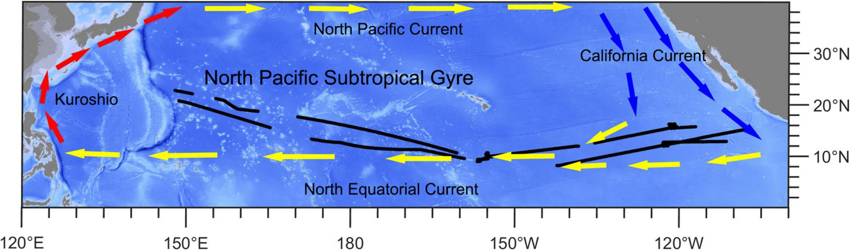
Ship-track (black lines) map of this study. Red arrows show the direction of the Kuroshio Current. Yellow arrows show the directions of the North Equatorial Current and North Pacific Current. Blue arrows show the direction of the California Current.
Ship-based data collection was conducted with a shipboard acoustic Doppler current profiler. The transducers (with a central frequency of 38 kHz) were mounted on the bottom of the ship. Datum was collected down to a depth of approximately 1,000. The sampling interval was 10 min, and the vertical cell interval was 24 m. A spline interpolation method was used to refine the raw data to 1 m vertical intervals (Akima, 1974). The measuring range was 50–1,000 m in depth. The raw acoustic data were not calibrated or compared with other calibrated equipment. However, the data from ship-board acoustic Doppler current profiler (SADCP) are considered suitable for evaluating the relative biomass of mesopelagic community and identifying the vertical distribution of DSLs in many studies (Irigoien et al., 2014; Davison et al., 2015; Bianchi and Mislan, 2016; Receveur et al., 2020a). Midday and midnight were defined as the periods of 10:00–14:00 and 20:00–02:00, respectively. Acoustic data of midday and midnight were used in the subsequent analysis because of the relatively stable scattering layers. This study focused on the mesopelagic zone (200–1,000 m underwater) to eliminate the influence of missing data from the 0–50-m zone. The mesopelagic zone is where the migratory organisms migrated into the DSLs at midday and migrated to surface at midnight.
Table 1 shows a list of abbreviations and full names in this study. The mean volume backscattering strength (MVBS, dB re 4Π m–1) was calculated from the recorded backscattering echo intensity E (counts) based on the sonar equation in Mullison (2017):
TABLE 1
| Acronyms | Full names | Unit |
| DSL | Deep scattering layers | \ |
| DVM | Diel vertical migration | \ |
| MVBS | Mean volume backscattering strength | dB re 4Πm–1 |
| VBC | Volume backscattering coefficient | m–1 |
| NASC | Nautical area scattering coefficient | m2 nmi–2 |
| UBD | Upper boundary depth | m |
| CM | Center mass | m |
| MP | Migration proportion | % |
| WMD | Weight migration depth | m |
| Chl a | Chlorophyll a | mg m–3 |
| LAC | Light attenuation coefficient | m–1 |
| MAT | Mesopelagic average temperature | °C |
| MAS | Mesopelagic average salinity | ‰ |
| MAO | Mesopelagic average oxygen | μmol kg–1 |
| WP | Western part | \ |
| TP | Transition part | \ |
| EP | Eastern part | \ |
List of abbreviation.
where Sv is the backscattering strength at a certain depth. C is a system constant provided by the SADCP manufacturer, which includes the transducer and system noise characteristics. This value is −172.19 dB for the Workhorse Long Ranger functioning at a frequency of 38 kHz. The other variables are as follows: Tx is the temperature of the transducer (°C), R is the range along the beam to the scatterers (m), LDBW is 10× lg (transmit pulse length, 24 m), PDBW is 24 dB, α is the sound absorption coefficient of seawater (0.011 dB m–1), and Kc is a beam-specific scaling factor (dB count–1), is typically assumed to be 0.45. Er is the received signal strength indicator value when there is no signal present, which is determined from the minimum values of the RSSI counts in the whole cruise (Deines, 1999; Mullison, 2017).
S v is the logarithmic form of sv (volume backscattering coefficient, VBC) in Equation 2, and sv is integrated with depth using the formula in Maclennan et al. (2002) to produce the area backscattering coefficient, sa (m2 m–2). The most common scaled coefficient, the nautical area scattering coefficient (NASC), is denoted by the symbol sA (m2 nmi–2) (Maclennan et al., 2002). The NASC calculated from the 38 kHz acoustic frequency was used as a proxy of micronekton biomass (Kloser et al., 2009; Béhagle et al., 2016).
where z is water depth (m), and sv (z) is the backscattering coefficient at depth z.
The threshold filtering method has been used in many studies to identify the location of DSLs (Béhagle et al., 2016; Klevjer et al., 2016). We used the threshold of −90 dB to identify DSLs in this study. It was based on agreement with visual inference and it is suitable according to the results (Netburn and Koslow, 2015). The upper boundaries and central depth of the DSLs (UBD and CM) were used to describe the vertical distribution of micronekton. The UBD was identified by the method modified from Netburn and Koslow (2015). The CM was derived for the DSLs using the approach provided by Urmy et al. (2012) as Equation 5.
where z represents the depths of layer, and sv (z) is the VBC at depth z.
The migrating proportion of mesopelagic organisms (MP) was calculated as the ratio of the difference between daytime and nighttime NASC (integrated from 200 to 1,000 m, average over the same day) to mesopelagic daytime NASC values. The mesopelagic weighted migration depth (WMD) was calculated as the weighted mean of the difference between daytime and nighttime mesopelagic NASC and depth in the mesopelagic zone (modified according to Klevjer et al., 2016).
where sA_day and sA_night were NASC (integrated from 200 to 1,000 m) at midday and midnight, respectively. i is the layer number of corresponding depth. sv_day(i) and sv_night(i) were the VBC at the i layer, at midday and midnight.
Environmental Data Collection and Processing
A suite of available environmental variables was selected to explore the environmental associations of DSLs. In this study, all environmental data were retrieved from public sources. The autumn average of chlorophyll a (Chl a) data with a 1/12° resolution were obtained from the NASA website.1 The autumn average of the 490-nm light attenuation coefficient (LAC) data with a 1/12° resolution were obtained from the NASA website (see text footnote 1). The LAC was calculated as Equation 8.
where k is LAC and depthx is a certain depth underwater. lightx and light0 are the light intensity at the certain depth underwater and surface light intensity, respectively (Padial and Thomaz, 2008).
The autumn average of the oceanic dissolved oxygen concentration, temperature and salinity profile data with a 1° resolution come from the world oceanic database (WOD2). The spline interpolation method was used to refine the profile data to 1-m intervals because the raw vertical resolution was not equally spaced. The mesopelagic (200–1,000 m) average temperature, salinity, and dissolved oxygen concentrations (MAT, MAS, and MAO) were calculated to describe the environment in the mesopelagic zone (Akima, 1974). The environmental data at the map grid point nearest to the acoustic location were used in subsequent processing.
Statistical Analysis
A k-means cluster analysis (Legendre and Legendre, 2012) of environmental variables (LAC, Chl a, MAT, MAO, MAS and the profile data of dissolved oxygen, salinity, and temperature) was used to divide the data into different groups. The number of clusters (k) was selected from a range between two and five to avoid excessive grouping without ecological significance. The result of cluster analysis was best when the k was three (Supplementary Figure 6).
The multiple regressions of DSL and environment (MAO, MAS, MAT, LAC, and Chl a) were conducted using the lme function of the mgcv R package (Lindstrom and Bates, 1988). First, we confirmed that collinearity was not apparent among the factors using variance inflation factors (VIFs) between each pair of covariates. The VIF implemented with the “car” library in R was used to evaluate the level of multicollinearity. Covariates were considered to be non-collinear when VIFs were less than 5 (O’brien, 2007; Boswell et al., 2020). The models were created by removing the high multicollinearity and non-significant parameters. The MAO and Chl a were ln transformed to satisfy the linear relationship between explanatory variables and response variables in the UBD, CM, and WMD models. Because the MP varied between 0 and 1, the Chl a in the model of MP was transformed into another nonlinear form. The explained variation of environmental factors to the dependent variable is expressed by R2.
Results
Longitudinal Environmental Gradient in the Tropical Pacific Ocean
The environment varied distinctly along the cruise track. Figure 2 shows that the mesopelagic region in the western tropical Pacific Ocean is a warm and oxygen-rich area with low productivity, while the eastern Pacific Ocean was a cold and hypoxia area with high productivity. The average mesopelagic oxygen concentration (MAO, 200–1,000 m) declined from 130 μmol kg–1 in the WP to 10 μmol kg–1 in the EP. The average mesopelagic temperature (MAT, 200–1,000 m) ranged of 9 to 7°C across the survey area (Figures 2A,C). The chlorophyll a concentration (Chl a) was higher in the eastern than the western tropical Pacific Ocean, varying from 0.15 to 0.03 mg m–3. The LAC had the same trend as Chl a, ranging from 0.038 to 0.02 m–1 from east to west (Figures 2D,E). Based on the result of cluster analysis, three environmental regions were identified: the WP (west of 175°E), the transition part (TP; from 175°E to 160°W), and the EP (east of 160°W) (Figure 2F). The chlorophyll a concentration in the EP was highest (0.072 ± 0.023 mg m–3) among these three regions. The chlorophyll a concentration in the TP (0.038 ± 0.005 mg m–3) was lower than that in the WP (0.040 ± 0.006 mg m–3). The MAO in the TP (48.2 ± 18.0 μmol kg–1) was intermediate between the WP (104.9 ± 14.7 μmol kg–1), and the EP (20.9 ± 7.4 μmol kg–1).
FIGURE 2
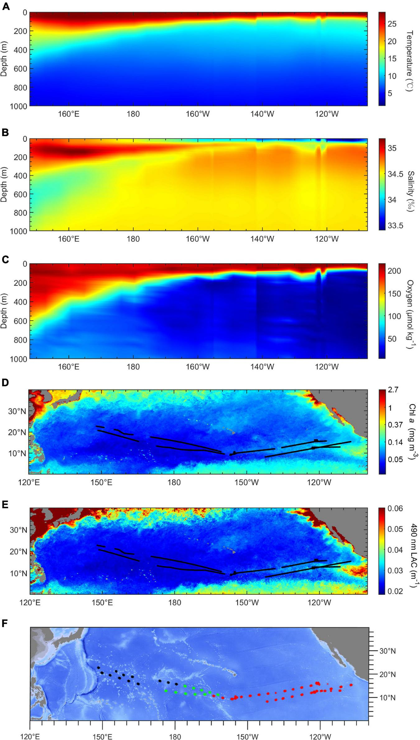
Environmental conditions in study area. (A–C) Profiles of temperature (°C), salinity (‰), and oxygen concentration (μmol kg– 1) in acoustic transects along a longitudinal gradient. (D,E) Maps of chlorophyll a concentration and 490-nm light attenuation coefficient (LAC, m– 1). (F) The result of k-means cluster analysis by environmental variables. Black, the western part (WP); green, the transition part (TP); red, the eastern part (EP).
Spatial Variations of Deep Scattering Layers and Diel Vertical Migration Along Longitudinal Gradient
At the trans-Pacific scale, the characteristics of DVM showed a clear diversity (Figure 3). The DSLs at noon were at depths between 450 and 750 m. The depths of surface scattering layers (SSLs) extended to more than 200 m below the surface at night in the western region (Figure 3A). The UBD became shallower eastward, but the cores of DSLs tended to diffuse downward (Figures 3B–D). In the eastern region, the DSLs were located at depths between 250 and 500 m at noon, and the depth of SSLs did not exceed the range of 100 m below the surface at night (Figure 3F).
FIGURE 3
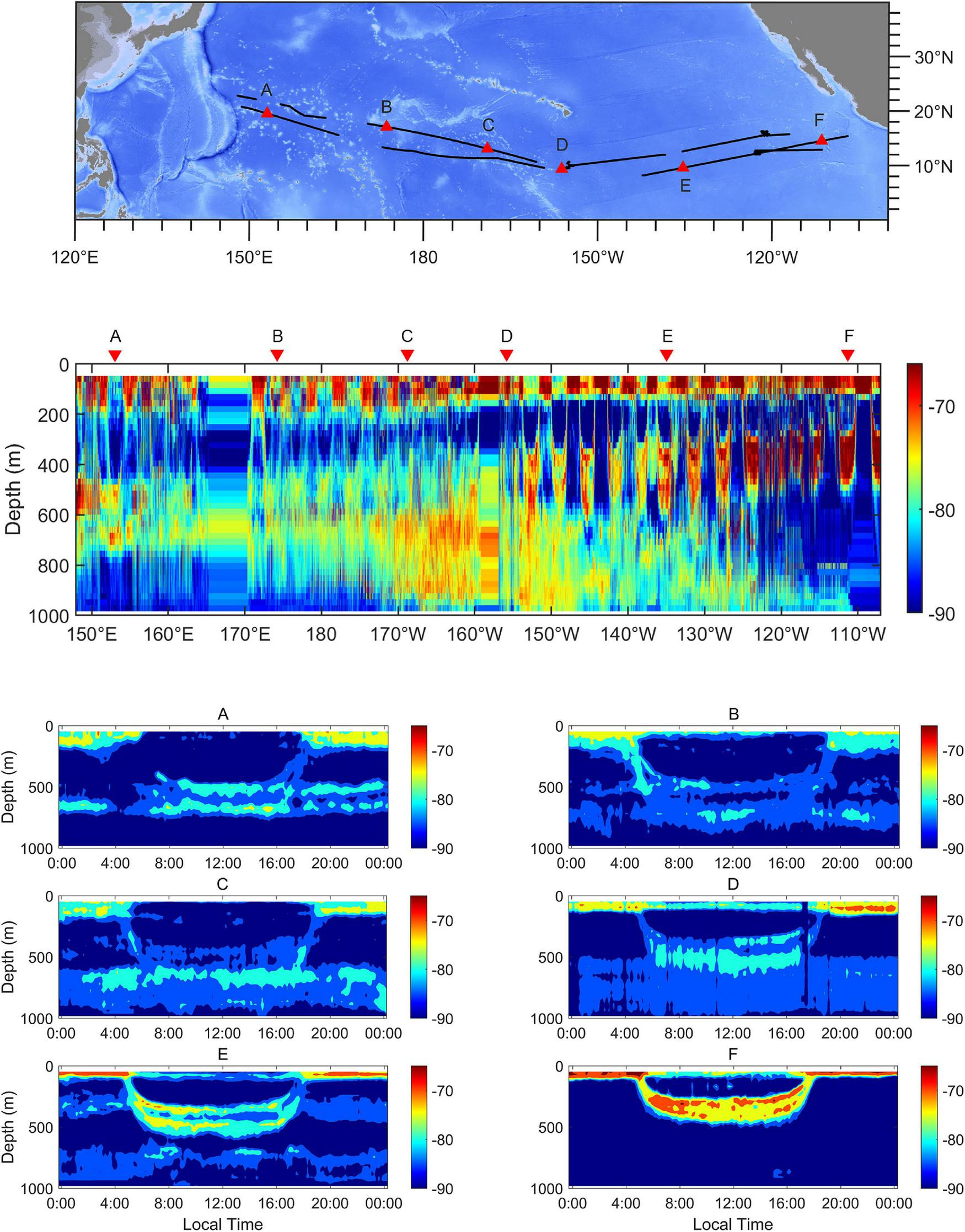
Echograms at 38 kHz across the tropical Pacific Ocean. The positions of examples are marked as triangles in the topographic map. The echograms show the spatial variation of DSLs, SSLs, and pattern of DVM from the western to the eastern tropical Pacific Ocean (A–F). Each echogram spans a 24-h period. The lower threshold was –90 dB. The ship-track was marked as black lines.
The vertical distribution of DSLs in three parts (WP, TP, and EP) is shown in Figure 4. The MP was highest in the EP (86.7 ± 16.2%, Figure 4D) where the WMD was shallowest (422.6 ± 80.8 m, Figure 4C). The WMD in the WP showed maximum depth (571.2 ± 85.5 m) among three parts (Figure 4C). The profiling data indicated that the DVM occurred mainly above 600 m and a significant non-migrative portion existed in the deeper layer (Figure 5). It is notable that the MP in the TP was minimum (35.2 ± 12.8%, Figure 4D), and the main body of DSLs was located below 600 m (Figure 5B). The vertical distribution characteristics of daytime DSLs along the longitudinal gradient are shown in Figure 6. The UBD gradually shallowed from 500 to 250 m, from the western to eastern Pacific Ocean. The CM was shallowest at 320 m on the eastern side, reached 720 m around 160°W, then rose to 500 m westward.
FIGURE 4
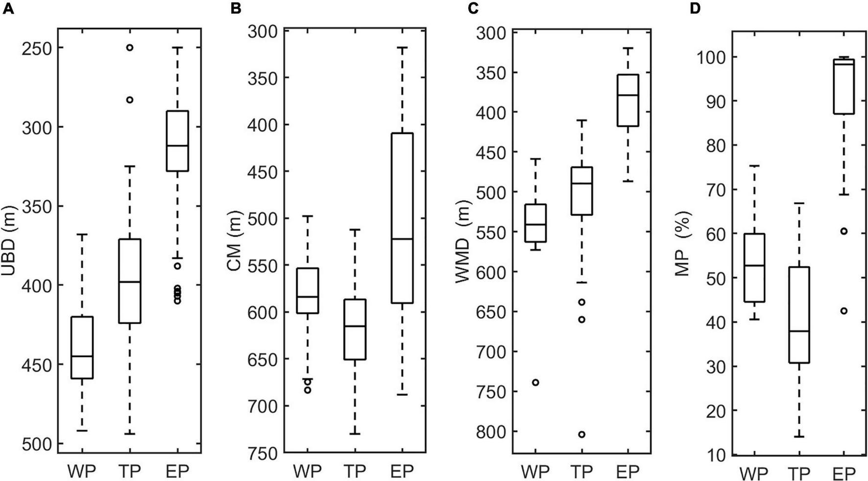
Box plots of the features of DSLs and DVMs, showing the differences among three parts. (A), UBD (m); (B), CM (m); (C) WMD (m); and (D), MP (%).
FIGURE 5
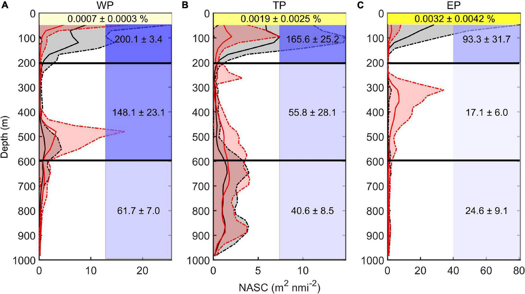
Vertical distribution of backscatter and environmental features. (A) Western part; (B) transition part; and (C) eastern part. Red lines showed the average midday-time profiles (10:00–14:00), red shadows were the range of standard deviations. Black lines showed the average midnight-time profiles (22:00–next day 2:00), gray shadows were the range of standard deviations. Yellow shadows represent the remaining light intensity (%) down to the WMD. Blue shadow in each grid represented the average oxygen concentration (μmol kg– 1; upper, 50–200 m; middle, 200–600 m; lower, 600–1000 m). The value (means ± SD) of environmental variable in each grid was also added.
FIGURE 6
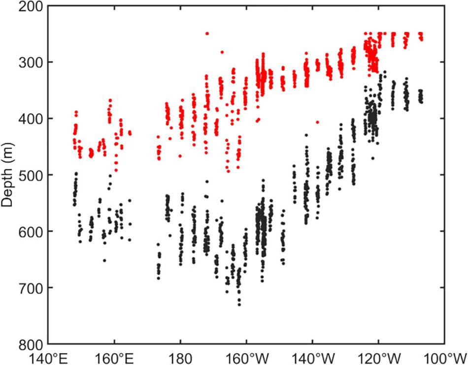
The vertical distribution of DSLs in daytime along the longitudinal gradient. The dots showed the UBD (red dots) and CM (black dots).
The Response of Deep Scattering Layers to Environment Gradient
The DSLs in the WP were mainly at the highest oxygen level (148.1 ± 23.1 μmol kg–1, average dissolved oxygen for 200–600 m, Figure 5A), which was about nine times as much as that in the EP (17.1 ± 6.0 μmol kg–1, average dissolved oxygen for 200–600 m, Figure 5C). In the TP, the main body of migration was located in a higher oxygen condition (55.8 ± 28.1 μmol kg–1, average dissolved oxygen for 200–600 m) than the non-migration area (40.6 ± 8.5 μmol kg–1, average dissolved oxygen for 600–1,000 m, Figure 5B). In the WP, the mesopelagic organisms migrated down to the weaker-light area (0.0007 ± 0.0003% surface light intensity, Figure 5A), while the light intensity was significantly higher at the depth of DSLs in the EP (0.0032 ± 0.0042% surface light intensity, Figure 5C). Two environmental variables (MAO and Chl a) were selected for modeling with DSLs and DVM by multicollinearity test (Supplementary Table 1). Details of the parameters and models were listed in Table 2; and the relationships between UBD, CM, WMD and MAO, Chl a were shown in Supplementary Figures 3–5, respectively.
TABLE 2
| Response variables | Explanatory variables | Estimates | Adj. R2 |
| UBD | ln (MAO) | 65.1*** | 0.77*** |
| ln (Chl a) | −32.5*** | ||
| CM | ln (Chl a) | −114.6*** | 0.72*** |
| WMD | ln (MAO) | 0.45** | 0.73*** |
| ln (Chl a) | −118.7*** | ||
| MP | 1/ (Chl a)2 | −0.087*** | 0.61*** |
Details of models, and variables used in models.
p-Value of each predictor are given as: **p < 0.01; ***p < 0.001.
For the UBD, both the MAO and Chl a explain 77% of the variation (UBD = 65.1 × ln (MAO) − 32.5 × ln (Chl a) + 26.1, n = 1104, p < 0.001, adj. R2 = 0.77). For the CM, the only significant explanatory factor was Chl a, explaining 72% of the variation (CM = −114.6 × ln (Chl a) − 224.9, n = 1104, p < 0.001, adj. R2 = 0.72). The WMD increased with increasing oxygen concentration, and decreased with increasing chlorophyll a (WMD = 0.45 × ln (MAO) − 118.7 × ln (Chl a) + 0.45, n = 63, p < 0.001, adj. R2 = 0.73). Only the Chl a was significant, explaining about 61% of the variation of MP (MP = −0.087 × 1 / (Chl a)2 + 100, n = 63, p < 0.001, adj. R2 = 0.61) (Figure 7).
FIGURE 7
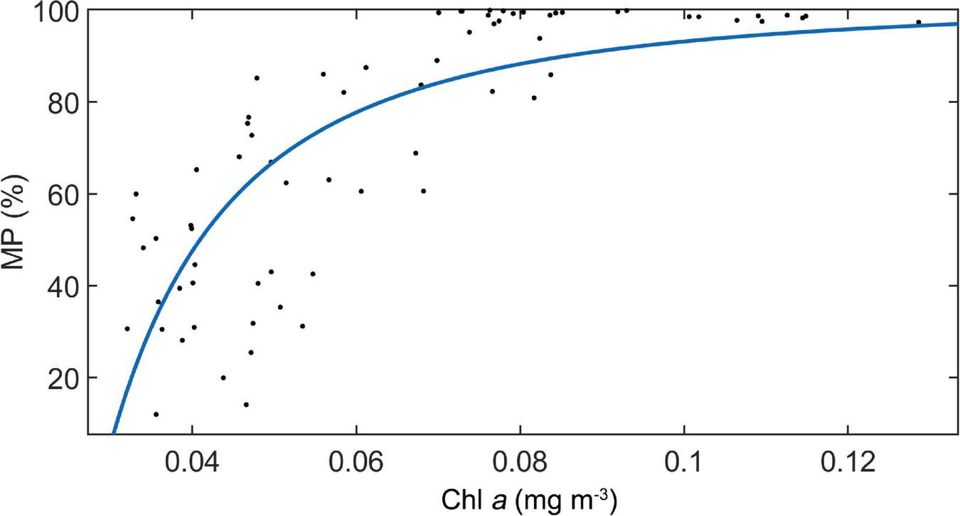
The relationship between MP and Chl a concentration along the ship-track in study area. A regression line was added.
Discussion
Longitudinal Environmental Gradient
According to the global biogeochemical classification of mesopelagic zone, the study area of tropical Pacific Ocean could be divided into three provinces from the western to the eastern: Subtropical Gyres Province, Tropical Province, and Subtropical Province (Reygondeau et al., 2017). According to another global biogeographic classification of mesopelagic zone, based not only on physical and biogeochemical data, but also on biome characteristics, the study area spanned two provinces: Northern Central Pacific Province and Eastern Tropical Pacific Province (Sutton et al., 2017). Both indicated the existence of significant large-scale environmental gradients. In the present study, this longitudinal environmental gradient was also confirmed. In addition, considering the continuous variation in the marine environment, this study also identifies a broad transition zone. The primary cause of this longitudinal environmental gradient in Pacific Ocean is biological oceanographic and biogeochemical mechanisms controlled by physical oceanographic differences, such as seasonal variation of mixed layer depth and transport of water masses (Amos et al., 2019; Diaz et al., 2021), but this environmental gradient is further reinforced by subtle biological processes, such as basin-scale distribution of nitrogen-fixing organisms (Cheung et al., 2020).
Spatial Variations of Deep Scattering Layers and Diel Vertical Migration Along Longitudinal Gradient in the Tropical Pacific Ocean
The mesopelagic community can be divided into two groups by their habitat and behavior: migrating organisms and non-migrating organisms (Salvanes and Kristoffersen, 2001; Bianchi and Mislan, 2016). These mesopelagic organisms have taxon-specific migration patterns and habitat depths, which result in significant spatial heterogeneity in the characteristics of DSLs. In a previous global-scale study, four DVM patterns were identified according to geographic regions: Atlantic Ocean, Indian Ocean, western and eastern Pacific Ocean (Klevjer et al., 2016). However, all these geographical DVM patterns were found in the present study. For example, the North Atlantic pattern, which was charactered by the DSLs with 400–600 m depth and smaller proportion of migrating mesopelagic organisms, was similar to the Figure 3A in the present study. The West Pacific pattern, which was charactered by the DSLs with 400–600 m depth and strong stratification of migrating and non-migrating organisms, was similar to the Figure 3D in the present study. The Indian pattern, which was charactered by the deeper DSLs with over 600 m depth, was similar to the Figure 3C in the present study. While the East Pacific pattern, which was charactered by the shallower DSLs with 200–500 m and larger proportion of migrating mesopelagic organisms, was similar to the Figure 3F in the present study (Bianchi et al., 2013; Netburn and Koslow, 2015; Bianchi and Mislan, 2016; Klevjer et al., 2016). This suggested that the spatial heterogeneity pattern of DVM was not as stable as previously thought and it was probably not reasonable to classify different distribution patterns based entirely on geographical distribution.
The composition of biome usually varies greatly under different environmental conditions (Whittaker et al., 1973; Dar et al., 2014). Although environmental conditions are more stable in the tropical open ocean than those in the coastal or offshore ecosystems, changes in dominant species with water mass may still exist on basin scale (Borgne et al., 2003; Christophe et al., 2015). The migratory mesopelagic fish includes only eight families (Myctophidae, Argentinidae, Sternoptychidae, Astronesthidae, Gonostomatidae, Melanostomiatidae, Stomiatidae, and Chauliodontidae) (Polis et al., 1997; Salvanes and Kristoffersen, 2001; Benoit-Bird and Lawson, 2016). In the tropical and subtropical waters, Myctophidae, Gonostomatidae, and Phosichthydae comprise most of the total catch, but the composition was various in different water masses (Brodeur and Yamamura, 2005). The dominant species in the western tropical Pacific Ocean was Myctophids (Gjøsaeter and Kawaguchi, 1980; Hidaka et al., 2001). The Myctophids, a group of migratory fish with swimming blabber, were also dominant in the biomass of mesopelagic community in the subtropical California Current system; while the Gonostomatidae were dominant in abundance (Davison et al., 2015). The DVM can be divided into three patterns based on environmental subregions in this study (Figures 2F, 5). From the migration proportion, it indicates that micronekton in the EP are almost entirely migrating species and the DSLs in the TP mainly consist of non-migrating species. Thus, although no net-collected sample was obtained in this study, the spatial heterogeneity of DSLs suggested that there was likely to be a longitudinal variation in mesopelagic community structure.
The Effect of Oxygen and Chlorophyll a on the Deep Scattering Layers and Diel Vertical Migration
The potential driving factors (such as primary production, dissolved oxygen, light intensity, temperature, and predation pressure) on the distribution of mesopelagic community and DSLs had been discussed in many previous studies (Pearre, 2003; Steinberg et al., 2008; Phillips et al., 2009; Staby et al., 2012; Escobar-Flores et al., 2013; Irigoien et al., 2014; Klevjer et al., 2016; Aksnes et al., 2017). These results suggested that the driving factors varied with the study scale and environmental background. In the present study, the dominant influencing factors were dissolved oxygen and chlorophyll concentration. We considered that this well reflected a trade-off between stress avoidance and energy intake.
Dissolved Oxygen
In this study, the mesopelagic zone (200–1,000 m) was divided into two parts according to the scattering vertical distribution at midday and midnight: the migrated part (200–600 m) and the stable part (600–1,000 m) (Figure 5). The DSLs of the EP are located where the dissolved oxygen was lowest in the study area (Figure 5C). The oxygen concentration is lower than the threshold (23 μmol kg–1), which probably limits the depth of DSLs in the California Current ecosystem (Netburn and Koslow, 2015). The DSLs are also mainly in the lower oxygen concentration region of the TP (Figure 5B). Considering the strong adaptation of micronekton to low oxygen conditions, this suggests that the micronekton may not select the higher oxygen condition as their shelter just because of metabolism constraints (Salvanes and Kristoffersen, 2001). However, dissolved oxygen can influence the depth of DVM in another way. As the results of the models show, the MAO influenced the UBD and WMD significantly. The UBD and WMD, which are both related to the DVM, represent the upper limit and center mass of DVM in our study. We assume that the oxygen drives the behavior of migratory micronekton by influencing the depth of predators. Tuna, the main fishery resource in the tropical Pacific Ocean, is the main predator of micronekton (Coull, 1993; Stramma et al., 2011; Macdonald et al., 2019; Moore et al., 2020; Post and Squires, 2020; Azmi and Hanich, 2021). They are more sensitive to oxygen concentration (>160 μmol kg–1) than micronekton due to the high oxygen consumption of their high-speed movement (Ingham et al., 1977; Cayré, 1991; Prince and Goodyear, 2006). Thus, a rise in dissolved oxygen concentration will increase the diving depth of predators, driving the micronekton migrating into deeper water.
Chlorophyll a
Chlorophyll a concentration is a good indicator of phytoplankton biomass in the open sea. Previous studies have well illustrated that the chlorophyll a concentration is closely related to primary productivity, and determines the biomass of micronekton based on bottom-up control mechanism (Shen and Shi, 2002; Escobar-Flores et al., 2013; Irigoien et al., 2014). Here, we proposed two other potential mechanisms for the effect of chlorophyll concentration on DSLs.
The first potential mechanism is about light attenuation by phytoplankton in water column. The phytoplankton is an important absorber of light in the water column (Stedmon and Nelson, 2015; Oestreich et al., 2016). There was a significant positive linear relationship between Chl a concentration and LAC in the study area (Figures 2D,E and Supplementary Figure 1). The transmission of light in water is poor. Generally, light loses 99% of its energy when it reaches mesopelagic zone (Phinney and Yentsch, 1986; Meadows and Campbell, 1993). Migratory mesopelagic fish have evolved an extraordinary sense of sight with large eyes and sensitive pure-rod retina (Salvanes and Kristoffersen, 2001). Non-migratory organisms do not have these characteristics. The visual threshold of predators is about 100 times higher than that of micronekton (Aksnes et al., 2017). Thus, there is a fitness advantage for micronekton to dive deeper during the day to avoid vision-dependent predators in more transparent environment (lower chlorophyll concentration).
The second potential mechanism is about lower energy demand of non-migratory organisms under poor food conditions. Since the metabolic rate of migratory organisms is always much higher than that of non-migratory organisms, the food demands of the former are significantly higher than those of the latter (Salvanes and Kristoffersen, 2001). This means that the migrating proportion of DSLs decreases in more oligotrophic environment, where species with high energy demands are restricted. In the present study, a significant positive relationship between MP and Chl a concentration well supported this hypothesis.
The Potential Change of Deep Scattering Layers and Mesopelagic Community Under Global Warming
Unlike occasional oceanographic disturbances, ocean warming is a long-term global process (Urmy and Horne, 2016). Ocean warming caused by global climate change will likely lead to ocean deoxygenation and ocean acidification (Reid et al., 2008; Stramma et al., 2008). Primary productivity has been predicted to decline in the tropical Pacific Ocean (Steinacher et al., 2010). These changes will modify the structure of marine ecosystems and their geochemical cycles (Karl, 1999; Jennings et al., 2008; Keeling et al., 2010; Pecl et al., 2017). On the one hand, previous studies predicated that the DSLs would be shallower because of ocean warming or ocean deoxygenation (Netburn and Koslow, 2015; Proud et al., 2017). On the other hand, the biomass of mesopelagic organisms would decrease with primary productivity (Steinacher et al., 2010; Irigoien et al., 2014). In the present study, we found that the migration proportion of mesopelagic organisms was positively related with chlorophyll a concentration in tropical Pacific Ocean, which is the third aspect of significant influence. Combining the result of previous studies and the findings of this study, it implied that declined biomass, shallower habituating depths, and lower migration proportion of mesopelagic animals under more extremely oligotrophic conditions with global change in future, which would reduce the active carbon flux (Anderson et al., 2019) and hinder food supply to deep-sea biological communities in the tropical Pacific Ocean (Ruhl and Smith, 2004).
The Limitation of This Study
A single frequency equipment at 38 kHz was used in this study, and it provided a remote view of the distribution of organisms in water. It should be considered that the acoustic intensity of object varies with the acoustic properties of organisms (the size and shape of body, the existence of swim bladder and shell), when the biomass of mesopelagic organisms was evaluated (Benoit-Bird and Lawson, 2016). Thus, the net collection of micronekton is valuable for this research. In our study, no samples were collected by net to measure the actual target strength unfortunately. However, it has been evident that acoustic survey method based on 38 kHz is effective in describing the population characteristics of micronekton and sound-scattering layers at large scale (Irigoien et al., 2014; Béhagle et al., 2016; Klevjer et al., 2016; Aksnes et al., 2017). More trawl surveys are still needed to analyze the longitudinal variations of micronekton community structure.
Conclusion
In this study, strong longitudinal variations of DSLs and DVM along the environment gradient across the tropical Pacific Ocean were found. The associations among the bio-acoustic and environmental variables suggested that the dissolved oxygen and light were the key factors to influence the depth of DSLs and migration. Since higher demand of most predators of mesopelagic animals for dissolved oxygen and light intensity, the limitations of predator behavior by environmental conditions might explain the observed spatial heterogeneity of DSLs. Combining the previous results and the findings of this study, it implied that declined biomass, shallower habituating depths, and lower migration proportion of mesopelagic animals under more extremely oligotrophic conditions with global change in future, would reduce the active carbon flux and hinder food supply to deep-sea biological communities in the tropical Pacific Ocean.
Publisher’s Note
All claims expressed in this article are solely those of the authors and do not necessarily represent those of their affiliated organizations, or those of the publisher, the editors and the reviewers. Any product that may be evaluated in this article, or claim that may be made by its manufacturer, is not guaranteed or endorsed by the publisher.
Statements
Data availability statement
The raw data supporting the conclusions of this article will be made available by the authors, without undue reservation.
Author contributions
DS and CW generated the research funding. YS analyzed the data with the help of DS and CW. YS and DS wrote the manuscript. All authors contributed to the article and approved the submitted version.
Funding
This work was funded by the National Natural Science Foundation of China (42076122), China Ocean Mineral Resources Research and Development Association Program (DY135-E2-3-04, DY135-E2-2-04), and Project of State Key Laboratory of Satellite Ocean Environment Dynamics, Second Institute of Oceanography (SOEDZZ2201).
Acknowledgments
We thank the three reviewers and the editor whose comments have greatly improved this manuscript. We also thank the members of R/V Xiangyanghong 10 for their help during the investigation.
Conflict of interest
The authors declare that the research was conducted in the absence of any commercial or financial relationships that could be construed as a potential conflict of interest.
Supplementary material
The Supplementary Material for this article can be found online at: https://www.frontiersin.org/articles/10.3389/fmars.2022.782032/full#supplementary-material
Footnotes
References
1
Akima H. (1974). A method of bivariate interpolation and smooth surface fitting based on local procedures.Commun. ACM1718–20. 10.1145/360767.360779
2
Aksnes D. L. Rostad A. Kaartvedt S. Martinez U. Duarte C. M. Irigoien X. (2017). Light penetration structures the deep acoustic scattering layers in the global ocean.Sci. Adv.3:1602468. 10.1126/sciadv.1602468
3
Amos C. M. Castelao R. M. Medeiros P. M. (2019). Offshore transport of particulate organic carbon in the California Current System by mesoscale eddies.Nat. Commun.10:4940. 10.1038/s41467-019-12783-5
4
Anderson T. R. Martin A. P. Lampitt R. S. Trueman C. N. Henson S. A. Mayor D. J. et al (2019). Quantifying carbon fluxes from primary production to mesopelagic fish using a simple food web model.ICES J. Mar. Sci.76690–701. 10.1093/icesjms/fsx234
5
Azmi K. Hanich Q. (2021). Mapping interests in the tuna fisheries of the western and Central Pacific ocean.Ocean Coast. Manag.212:105779. 10.1016/j.ocecoaman.2021.105779
6
Beaugrand G. Reid P. C. Ibanez F. Lindley J. A. Edwards M. (2002). Reorganization of North Atlantic marine copepod biodiversity and climate.Science2961692–1694. 10.1126/science.1071329
7
Béhagle N. Cotté C. Ryan T. E. Gauthier O. Roudaut G. Brehmer P. et al (2016). Acoustic micronektonic distribution is structured by macroscale oceanographic processes across 20–50°S latitudes in the South-Western Indian Ocean.Deep Sea Res. Part I Oceanogr. Res. Pap.11020–32. 10.1016/j.dsr.2015.12.007
8
Béhagle N. Du Buisson L. Josse E. Lebourges-Dhaussy A. Roudaut G. Ménard F. (2014). Mesoscale features and micronekton in the Mozambique channel: an acoustic approach.Deep Sea Res. Part II Top Stud. Oceanogr.100164–173. 10.1016/j.dsr2.2013.10.024
9
Benedetti F. Vogt M. Elizondo U. H. Righetti D. Zimmermann N. E. Gruber N. (2021). Major restructuring of marine plankton assemblages under global warming.Nat. Commun.12:5226. 10.1038/s41467-021-25385-x
10
Benoit-Bird K. J. Lawson G. L. (2016). Ecological insights from pelagic habitats acquired using active acoustic techniques.Ann. Rev. Mar. Sci.8463–490. 10.1146/annurev-marine-122414-034001
11
Bertrand A. Bard F.-X. Josse E. (2002). Tuna food habits related to the micronekton distribution in French Polynesia.Mar. Biol.1401023–1037. 10.1007/s00227-001-0776-3
12
Bianchi D. Mislan K. A. S. (2016). Global patterns of diel vertical migration times and velocities from acoustic data.Limnol. Oceanogr.61353–364. 10.1002/lno.10219
13
Bianchi D. Galbraith E. D. Carozza D. A. Mislan K. A. S. Stock C. A. (2013). Intensification of open-ocean oxygen depletion by vertically migrating animals.Nat. Geosci.6545–548. 10.1038/ngeo1837
14
Borgne R. L. Champalbert G. L. Gaudy R. (2003). Mesozooplankton biomass and composition in the equatorial Pacific along 180°.J. Geophys. Res.108:8143. 10.1029/2000JC000745
15
Boswell K. M. D’elia M. Johnston M. W. Mohan J. A. Warren J. D. Wells R. J. D. et al (2020). Oceanographic structure and light levels drive patterns of sound scattering layers in a low-latitude oceanic system.Front. Mar. Sci.7:e051. 10.3389/fmars.2020.00051
16
Brodeur R. D. Yamamura O. (2005). Micronekton of the North Pacific.PICES Sci. Rep.301–115. 10.1002/lno.11128
17
Cascão I. Domokos R. Lammers M. O. Santos R. S. Silva M. A. (2019). Seamount effects on the diel vertical migration and spatial structure of micronekton.Prog. Oceanogr.1751–13. 10.1016/j.pocean.2019.03.008
18
Catul V. Gauns M. Karuppasamy P. K. (2010). A review on mesopelagic fishes belonging to family Myctophidae.Rev. Fish. Biol. Fish.21339–354. 10.1007/s11160-010-9176-4
19
Cayré P. (1991). Behavior of yellowfin tuna (Thunnus albacares) and skipjack tuna (Katsuwonus pelamis) around fish aggregating devices (FADs) in the Comoros Islands as determined by ultrasonic tagging.Aquat. Living Resour.41–12. 10.1051/alr/1991000
20
Cheung S. Nitanai R. Tsurumoto C. Endo H. Nakaoka S. I. Cheah W. et al (2020). Physical forcing controls the basin-scale occurrence of nitrogen-fixing organisms in the North Pacific Ocean.Global Biogeochem. Cycles34:e2019GB006452. 10.1029/2019gb006452
21
Christophe M. Rachid A. Mario L. (2015). “Fish as Reference Species in Different Water Masses,” in Aquatic Ecotoxicology:Advancing Tools for Dealing with Emerging Risks, ed.Amiard-TriquetC. (Boca Raton, FL: CRC Press), 309–331. 10.1016/b978-0-12-800949-9.00013-9
22
Claustre H. Maritorena S. (2003). The many shades of ocean blue.Science3021514–1515. 10.1126/science.1092704
23
Coull J. R. (1993). World Fisheries Resources.London: Routledge.
24
Dar N. A. Pandit A. K. Ganai B. A. (2014). Factors affecting the distribution patterns of aquatic macrophytes.Limnol. Rev.1475–81. 10.2478/limre-2014-0008
25
Davison P. Lara-Lopez A. Anthony Koslow J. (2015). Mesopelagic fish biomass in the southern California current ecosystem.Deep Sea Res. Part II Top Stud. Oceanogr.112129–142. 10.1016/j.dsr2.2014.10.007
26
De Robertis A. Cokelet E. D. (2012). Distribution of fish and macrozooplankton in ice-covered and open-water areas of the eastern Bering Sea.Deep Sea Res. Part II Top Stud. Oceanogr.65-70217–229. 10.1016/j.dsr2.2012.02.005
27
Deines K. L. (1999). “Backscatter estimation using broadband acoustic doppler current profilers,” in Proceedings of the 6th IEEE Working Conference on Current Measurement (San Diego, CA), 249–253. 10.1109/CCM.1999.755249
28
Diaz B. P. Knowles B. Johns C. T. Laber C. P. Bondoc K. G. V. Haramaty L. et al (2021). Seasonal mixed layer depth shapes phytoplankton physiology, viral production, and accumulation in the North Atlantic.Nat. Commun.12:6634. 10.1038/s41467-021-26836-1
29
Escobar-Flores P. O’driscoll R. L. Montgomery J. C. (2013). Acoustic characterization of pelagic fish distribution across the South Pacific Ocean.Mar. Ecol. Prog. Ser.490169–183. 10.3354/meps10435
30
Fennell S. Rose G. (2015). Oceanographic influences on Deep Scattering Layers across the North Atlantic.Deep Sea Res. Part I Oceanogr. Res. Pap.105132–141. 10.1016/j.dsr.2015.09.002
31
Food and Agriculture Organization [FAO] (2018). The State of World Fisheries and Aquaculture.Rome: F.A.O Fisheries and Aquaculture Department.
32
Gjøsaeter J. Kawaguchi K. (1980). A review of the world resources of mesopelagic fish.FAO Fish. Tech. Pap.1391–134.
33
Hays G. C. (2003). A review of the adaptive significance and ecosystem consequences of zooplankton diel vertical migrations.Hydrobiologia503163–170. 10.1023/B:HYDR.0000008476.23617.b0
34
He Q. Zhan H. Cai S. Zha G. (2016). On the asymmetry of eddy-induced surface chlorophyll anomalies in the southeastern Pacific: the role of eddy-Ekman pumping.Prog. Oceanogr.141202–211. 10.1016/j.pocean.2015.12.012
35
Hernández-León S. Olivar M. P. Fernández De Puelles M. L. Bode A. Castellón A. López-Pérez C. et al (2019). Zooplankton and micronekton active flux across the tropical and subtropical Atlantic Ocean.Front. Mar. Sci.6:535. 10.3389/fmars.2019.00535
36
Hidaka K. Kawaguchi K. Murakami M. Takahashi M. (2001). Downward transport of organic carbon by diel migratory micronekton in the western equatorial Pacic: its quantitative and qualitative importance.Deep Sea Res. Part I Oceanogr. Res. Pap.481923–1939. 10.1016/S0967-0637(01)00003-6
37
Hu D. Wu L. Cai W. Gupta A. S. Ganachaud A. Qiu B. et al (2015). Pacific western boundary currents and their roles in climate.Nature522299–308. 10.1038/nature14504
38
Ingham M. C. Cook S. K. Hausknecht K. A. (1977). Oxycline characteristics and skipjack tuna distribution in the southeastern tropical Atlantic.Fish. Bull.75857–865.
39
Irigoien X. Klevjer T. A. Rostad A. Martinez U. Boyra G. Acuna J. L. et al (2014). Large mesopelagic fishes biomass and trophic efficiency in the open ocean.Nat. Commun.5:3271. 10.1038/ncomms4271
40
Jennings S. Me’Lin F. D. R. Blanchard J. L. Forster R. M. Dulvy N. K. Wilson R. W. (2008). Global-scale predictions of community and ecosystem properties from simple ecological theory.Proc. R. Soc. Lond. B Biol. Sci.2751375–1383. 10.1098/rspb.2008.0192
41
Johnson M. W. (1948). Sound as a tool in marine ecology, from data on biological noises and the deep scattering layer.J. Mar. Res.7443–458.
42
Kaartvedt S. Staby A. Aksnes D. L. (2012). Efficient trawl avoidance by mesopelagic fishes causes large underestimation of their biomass.Mar. Ecol. Prog. Ser.4561–6. 10.3354/meps09785
43
Karl D. M. (1999). A sea of change: biogeochemical variability in the North Pacific Subtropical Gyre.Ecosystems2181–214. 10.1007/s100219900068
44
Keeling R. E. Kortzinger A. Gruber N. (2010). Ocean deoxygenation in a warming world.Ann. Rev. Mar. Sci.2199–229. 10.1146/annurev.marine.010908.163855
45
Klevjer T. A. Irigoien X. Røstad A. Fraile-Nuez E. (2016). Large scale patterns in vertical distribution and behaviour of mesopelagic scattering layers.Sci. Rep.6:19873. 10.1038/srep19873
46
Klevjer T. Melle W. Knutsen T. Strand E. Korneliussen R. Dupont N. et al (2019). Micronekton biomass distribution, improved estimates across four north Atlantic basins.Deep Sea Res. Part II Top Stud. Oceanogr.180:104691. 10.1016/j.dsr2.2019.104691
47
Kloser R. J. Ryan T. E. Young J. W. Lewis M. E. (2009). Acoustic observations of micronekton fish on the scale of an ocean basin: potential and challenges.ICES J. Mar. Sci.66998–1006. 10.1093/icesjms/fsp077
48
Kunreuther H. Gupta S. Bosetti V. Cooke R. Dutt V. Ha-Duong M. et al (2014). “Integrated risk and uncertainty assessment of climate change response policies,” in Proceedings of theClimate Change 2014: Mitigation of Climate Change Contribution of Working Group III to the Fifth Assessment Report of the Intergovernmental Panel on Climate Change, ed.EdenhoferO. (New York, NY: Cambridge University Press), 151–206. 10.1017/cbo9781107415416.008
49
Kwong L. E. Henschke N. Pakhomov E. A. Everett J. D. Suthers I. M. (2020). Mesozooplankton and Micronekton Active Carbon Transport in Contrasting Eddies.Front. Mar. Sci.6:00825. 10.3389/fmars.2019.00825
50
Lambert C. Mannocci L. Lehodey P. Ridoux V. (2014). Predicting cetacean habitats from their energetic needs and the distribution of their prey in two contrasted tropical regions.PLoS One9:e105958. 10.1371/journal.pone.0105958
51
Le Borgne R. Barber R. T. Delcroix T. Inoue H. Y. Mackey D. J. Rodier M. (2002). Pacific warm pool and divergence: temporal and zonal variations on the equator and their effects on the biological pump.Deep Sea Res. Part II Top. Stud. Oceanogr.492471–2512. 10.1016/S0967-0645(02)00045-0
52
Legendre P. Legendre L. (2012). Numerical Ecology (3rd English edition).Amsterdam: Elsevier.
53
Levin L. A. (2003). Oxygen minimum zone benthos: adaptation and community response to hypoxia.Oceanogr. Mar. Biol.411–45.
54
Lindstrom M. J. Bates D. M. (1988). Newton-raphson and EM algorithms for linear mixed-effects models for repeated-measures data. J Am. Stat. Assoc.83, 1014–1022. 10.1080/01621459.1988.10478693
55
Macdonald J. I. Moore B. Smith N. (2019). “Stock structure considerations for Pacific Ocean tunas,” in Proceedings of the 15th regular session of the Scientific Committee of the Western and Central Pacific Fisheries Commission, Pohnpei.
56
Maclennan D. Fernandes P. G. Dalen J. (2002). A consistent approach to definitions and symbols in fisheries acoustics. ICES J. Mar. Sci.59, 365–369. 10.1006/jmsc.2001.1158
57
Martin A. Boyd P. Buesseler K. Cetinic I. Claustre H. Giering S. et al (2020). The oceans’ twilight zone must be studied now, before it is too late.Nature58026–28. 10.1038/d41586-020-00915-7
58
Meadows P. S. Campbell J. I. (1993). A Introduction to Marine Science.London: Blackie Academic & Professional.
59
Miller M. G. R. Carlile N. Scutt Phillips J. Mcduie F. Congdon B. C. (2018). Importance of tropical tuna for seabird foraging over a marine productivity gradient.Mar. Ecol. Prog. Ser.586233–249. 10.3354/meps12376
60
Moline M. A. Benoit-Bird K. O’gorman D. Robbins I. C. (2015). Integration of scientific echo sounders with an adaptable autonomous vehicle to extend our understanding of animals from the surface to the bathypelagic.J. Atmos. Ocean Technol.322173–2186. 10.1175/jtech-d-15-0035.1
61
Moore B. R. Adams T. Allain V. Bell J. D. Bigler M. Bromhead D. et al (2020). Defining the stock structures of key commercial tunas in the Pacific Ocean II: sampling considerations and future directions.Fish. Res.230:105524. 10.1016/j.fishres.2020.105524
62
Mullison J. (2017). “Backscatter estimation using broadband acoustic doppler current profilers – updated,” in Hydraulic Measurements & Experimental Methods Conference (Durham, NH).
63
Netburn A. N. Koslow A. J. (2015). Dissolved oxygen as a constraint on daytime deep scattering layer depth in the southern California current ecosystem.Deep Sea Res. Part I Oceanogr. Res. Pap.104149–158. 10.1016/j.dsr.2015.06.006
64
O’brien R. M. (2007). A caution regarding rules of thumb for variance inflation factors.Qual. Quant.41673–690. 10.1007/s11135-006-9018-6
65
Oestreich W. Ganju N. Pohlman J. Suttles S. E. (2016). Colored dissolved organic matter in shallow estuaries: relationships between carbon sources and light attenuation.Biogeosciences13583–595. 10.5194/bg-13-583-2016
66
Padial A. A. Thomaz S. M. (2008). Prediction of the light attenuation coefficient through the Secchi disk depth: empirical modeling in two large Neotropical ecosystems. Limnology9, 143–151. 10.1007/s10201-008-0246-4
67
Pearre S. (2003). Eat and run? The hunger/satiation hypothesis in vertical migration: history, evidence and consequences.Biol. Rev.781–79. 10.1002/lno.10606
68
Pecl G. T. Araujo M. B. Bell J. D. Blanchard J. Bonebrake T. C. Chen I. C. et al (2017). Biodiversity redistribution under climate change: impacts on ecosystems and human well-being.Science355:eaai9214. 10.1126/science.aai9214
69
Phillips J. Brodeur R. Suntsov A. (2009). Micronekton community structure in the epipelagic zone of the northern California Current upwelling system.Prog. Oceanogr.8074–92. 10.1016/j.pocean.2008.12.001
70
Phinney D. A. Yentsch C. S. (1986). The Relationship Between Phytoplankton Concentration and Light Attenuation in Ocean Waters.Ocean. Opt.637321–327. 10.1117/12.964248
71
Polis G. A. Anderson W. B. Holt R. D. (1997). Toward an integration of landscape and food web ecology: the dynamics of spatially subsidized food webs.Annu. Rev. Ecol. Syst.28289–316. 10.1146/annurev.ecolsys.28.1.289
72
Post V. Squires D. (2020). Managing Bigeye Tuna in the Western and Central Pacific Ocean.Front. Mar. Sci.7:619. 10.3389/fmars.2020.00619
73
Prince E. D. Goodyear C. P. (2006). Hypoxia-based habitat compression of tropical pelagic fishes.Fish. Oceanogr.15451–464. 10.1111/j.1365-2419.2005.00393.x
74
Proud R. Cox M. J. Brierley A. S. (2017). Biogeography of the Global Ocean’s mesopelagic zone.Curr. Biol.27113–119. 10.1016/j.cub.2016.11.003
75
Receveur A. Kestenare E. Allain V. Ménard F. Cravatte S. Lebourges-Dhaussy A. et al (2020a). Micronekton distribution in the southwest Pacific (New Caledonia) inferred from shipboard-ADCP backscatter data.Deep Sea Res. Part I Oceanogr. Res. Pap.159:103237. 10.1016/j.dsr.2020.103237
76
Receveur A. Vourey E. Lebourges-Dhaussy A. Menkes C. Ménard F. Allain V. (2020b). Biogeography of micronekton assemblages in the Natural Park of the Coral Sea.Front. Mar. Sci.7:449. 10.3389/fmars.2020.00449
77
Reid P. C. Andersson A. Arthurton R. Bates N. Barange M. Bathmann U. et al (2008). “The Impacts of the Oceans on Climate Change,” in Proceedings of the 2nd Electronics System Integration Technology Conference, Greenwich, 29–32.
78
Resplandy L. (2018). Will ocean zones with low oxygen levels expand or shrink?Nature557314–315. 10.1002/2017gb005788
79
Reygondeau G. Guidi L. Beaugrand G. Henson S. A. Koubbi P. Mackenzie B. R. et al (2017). Global biogeochemical provinces of the mesopelagic zone.J. Biogeogr.45500–514. 10.1111/jbi.13149
80
Ruhl H. A. Smith K. L. Jr. (2004). Shifts in deep-sea community structure linked to climate and food supply.Science305513–515. 10.1126/science.1099759
81
Salvanes A. G. V. Kristoffersen J. B. (2001). “Mesopelagic fishes,” in Encyclopedia of Ocean Science, ed.SteeleJ. (Cambridge, MA: Academic Press), 1711–1717. 10.1006/rwos.2001.0012
82
Shen G. Shi B. (2002). Primary Production in Marine.Beijing: Science Press.
83
Smeti H. Pagano M. Menkes C. Lebourges-Dhaussy A. Hunt B. P. V. Allain V. et al (2015). Spatial and temporal variability of zooplankton off New Caledonia (Southwestern Pacific) from acoustics and net measurements.J. Geophys. Res. Oceans1202676–2700. 10.1002/2014jc010441
84
Staby A. Srisomwong J. Rosland R. (2012). Variation in DVM behaviour of juvenile and adult pearlside (Maurolicus muelleri) linked to feeding strategies and related predation risk.Fish. Oceanogr.2290–101. 10.1111/fog.12012
85
Stedmon C. Nelson N. (2015). “The optical properties of DOM in the Ocean,” in Biogeochemistry of Marine Dissolved Organic Matter, edsHansellD. A.CarlsonC. A. (Amsterdam: Elsevier), 481–508.
86
Steinacher M. Joos F. Frölicher T. L. Bopp L. Cadule P. Cocco V. et al (2010). Projected 21st century decrease in marine productivity: a multi-model analysis.Biogeosciences7979–1005. 10.5194/bg-7-979-2010
87
Steinberg D. K. Cope J. S. Wilson S. E. Kobari T. (2008). A comparison of mesopelagic mesozooplankton community structure in the subtropical and subarctic North Pacific Ocean.Deep Sea Res. Part II Top. Stud. Oceanogr.551615–1635. 10.1016/j.dsr2.2008.04.025
88
Stramma L. Johnson G. C. Sprintall J. Mohrholz V. (2008). Expanding oxygen-minimum zones in the tropical oceans.Science320655–658. 10.1126/science.1153847
89
Stramma L. Prince E. D. Schmidtko S. Luo J. Hoolihan J. P. Visbeck M. et al (2011). Expansion of oxygen minimum zones may reduce available habitat for tropical pelagic fishes.Nat. Clim. Chang.233–37. 10.1038/nclimate1304
90
Sutton T. T. Clark M. R. Dunn D. C. Halpin P. N. Rogers A. D. Guinotte J. et al (2017). A global biogeographic classification of the mesopelagic zone.Deep Sea Res. Part I Oceanogr. Res. Pap.12685–102. 10.1016/j.dsr.2017.05.006
91
Urmy S. S. Horne J. K. Barbee D. H. (2012). Measuring the vertical distributional variability of pelagic fauna in Monterey Bay. ICES J. Mar. Sci.69, 184–196. 10.1093/icesjms/fsr205
92
Urmy S. S. Horne J. K. (2016). Multi-scale responses of scattering layers to environmental variability in Monterey Bay, California.Deep Sea Res. Part I Oceanogr. Res. Pap.11322–32. 10.1016/j.dsr.2016.04.004
93
Wang F. Wang Q. Zhang L. Hu D. Hu S. Feng J. (2019). Spatial distribution of the seasonal variability of the North Equatorial Current.Deep Sea Res. Part I Oceanogr. Res. Pap.14463–74. 10.1016/j.dsr.2019.01.001
94
Whittaker R. H. Levin S. A. Root R. B. (1973). Niche, Habitat, and Ecotope.Am. Nat.107321–338. 10.1086/282837
95
Zhang D. Wang C. Liu Z. Xu X. Wang X. Zhou Y. (2012). Spatial and temporal variability and size fractionation of chlorophyll a in the tropical and subtropical Pacific Ocean.Acta Oceanol. Sin.31120–131. 10.1007/s13131-012-0212-1
Summary
Keywords
deep scattering layer, mesopelagic community, diel vertical migration, carbon pump, climate change
Citation
Song Y, Wang C and Sun D (2022) Both Dissolved Oxygen and Chlorophyll Explain the Large-Scale Longitudinal Variation of Deep Scattering Layers in the Tropical Pacific Ocean. Front. Mar. Sci. 9:782032. doi: 10.3389/fmars.2022.782032
Received
23 September 2021
Accepted
09 February 2022
Published
11 March 2022
Volume
9 - 2022
Edited by
Angel Borja, Technological Center Expert in Marine and Food Innovation (AZTI), Spain
Reviewed by
Kusum Komal Karati, Centre for Marine Living Resources and Ecology (CMLRE), India; Roland Proud, University of St Andrews, United Kingdom; Ivan Pérez-Santos, University of Los Lagos, Chile
Updates
Copyright
© 2022 Song, Wang and Sun.
This is an open-access article distributed under the terms of the Creative Commons Attribution License (CC BY). The use, distribution or reproduction in other forums is permitted, provided the original author(s) and the copyright owner(s) are credited and that the original publication in this journal is cited, in accordance with accepted academic practice. No use, distribution or reproduction is permitted which does not comply with these terms.
*Correspondence: Dong Sun, sund@sio.org.cn
This article was submitted to Marine Ecosystem Ecology, a section of the journal Frontiers in Marine Science
Disclaimer
All claims expressed in this article are solely those of the authors and do not necessarily represent those of their affiliated organizations, or those of the publisher, the editors and the reviewers. Any product that may be evaluated in this article or claim that may be made by its manufacturer is not guaranteed or endorsed by the publisher.