Abstract
Intraseasonal Kelvin waves (IKWs) and Tropical Instability Waves (TIWs) are essential components of the tropical Pacific coupled climate variability. While downwelling IKWs are precursors of ENSO (e.g., the El Niño Southern Oscillation), TIWs contribute to its asymmetry by mixing more/less warm off-equatorial and cold tongue waters during La Niña/El Niño. Theoretical studies and a few observational case studies also suggest that TIWs and IKWs can interact non-linearly. However, owing to the chaotic nature of TIWs, observational evidence that such a process occurs consistently has not been established thus far. Here, we document for the first time their interaction from satellite observations over a period spanning almost 30 years (1993–2018). From complex empirical orthogonal functions analysis and sea level decomposition into meridional modes, we evidence that a substantial share (∼42%) of the variance of TIWs-induced intraseasonal sea level anomalies are associated with IKWs activity. We show that non-linear dynamical heating (NDH) in the Eastern equatorial Pacific associated with this intraseasonal mode can be as large as that for interannual time scales. Implications for understanding the eastern tropical Pacific heat budget and ENSO variability are discussed.
Introduction
Tropical instability waves (TIWs) are unique westward-moving cusp-shaped mesoscale features first observed via infrared satellite systems by Legeckis (1977) in particular along the strong meridional Sea Surface Temperature (SST) gradient in the eastern equatorial Pacific. Thereafter, TIWs signature has also been observed in many other ocean-surface variables such as sea surface height (Lawrence and Angell, 2000; Benestad et al., 2001; Polito et al., 2001; Lyman et al., 2005; Shinoda et al., 2009), meridional and zonal velocity (Qiao and Weisberg, 1995; Flament et al., 1996; Inoue et al., 2012), salinity (Lee et al., 2012), ocean color (Yoder et al., 1994; Strutton et al., 2001; Legeckis et al., 2004; Evans et al., 2009), subsurface temperature (Flament et al., 1996; McPhaden, 1996; Kennan and Flament, 2000) and even atmospheric variables such as low-level wind and wind stress (Xie et al., 1998; Chelton et al., 2001; Hashizume et al., 2001).
This dominant form of eddy variability in the near equatorial region can modulate many aspects of the basin-scale equatorial circulation. For instance, TIWs-induced upwelling has been suggested to fertilize the central equatorial region (Yoder et al., 1994; Strutton et al., 2001; Menkes, 2002), which is related to the vigorous turbulent mixing and associated vertical heat flux they produce at their leading edges (Dutrieux et al., 2008; Lien et al., 2008; Moum et al., 2009; Inoue et al., 2012; Holmes and Thomas, 2015; Liu et al., 2016; Warner et al., 2018). TIWs are also thought to modulate the mixed-layer heat budget at seasonal to interannual time scales (Jochum and Murtugudde, 2006; Menkes et al., 2006), potentially affecting longer time scales of variability through the modulation of air–sea interactions at basin-scale. In particular, the enhanced meridional heat transport associated with TIWs during La Niña; compared to El Niño has been shown to contribute to the El Niño–Southern Oscillation (ENSO) asymmetry characterized by larger-amplitude El Niño than La Niña events (An, 2008; Imada and Kimoto, 2012; Boucharel and Jin, 2020; Xue et al., 2020, 2021), which can in turn feedback onto the Pacific decadal variability (Rodgers et al., 2004; Yeh and Kirtman, 2004, 2005; Choi et al., 2009, 2011, 2013; Ogata et al., 2013; Capotondi et al., 2020; Zhao et al., 2021). TIWs have also been suggested to modulate the subthermocline circulation by radiating internal waves downward (Jing et al., 2014; Holmes and Thomas, 2016; Tanaka and Hibiya, 2019; Delpech et al., 2020), which also represents a pathway by which TIWs could influence long-term climate variability. Despite their likely importance on the global climate, TIWs are still not simulated to the full extent of their observed characteristics in IPCC (Intergovernmental Panel on Climate Change)-like models, mostly due to their too coarse horizontal resolution. Most studies have thus focused on how mean state change can modulate TIWs activities from high-to-medium resolution simulations of ocean general circulation models (Pezzi, 2003; Zhang, 2014).
As they are generated in part by barotropic energy conversion associated with the large meridional shears between the North Equatorial Counter Current (NECC) and South Equatorial Current (Philander, 1978; Cox, 1980; Imada and Kimoto, 2012) and between the Equatorial Undercurrent (EUC) and South Equatorial Current (SEC) (Luther and Johnson, 1990; Lyman et al., 2007), TIWs activity depends on the state of these equatorial currents and the associated thermocline structure. Such large-scale equatorial circulation features are modulated among others by planetary equatorial waves. For instance, during a La Niña event, the equatorial upwelling Kelvin waves tend to sharpen/uplift the central equatorial thermocline and intensify the EUC (Izumo et al., 2002; Izumo, 2005; Roundy and Kiladis, 2006; Rydbeck et al., 2019) which favors the growth of an unstable linear mode associated with the coupling of two Rossby waves, that are trapped along the latitudinal bands of ∼1–3°N and ∼3–8°N, respectively (Tanaka and Hibiya, 2019). TIWs can thus be seen in part as the result of these two Rossby waves interacting with off-equatorial currents with a westward propagation and growth rate of TIWs (Lawrence et al., 1998; Tanaka and Hibiya, 2019). On the other hand, during the peak phase of strong El Niño events, reflected downwelling equatorial Rossby waves at the eastern boundary can reduce the NECC (Hsin and Qiu, 2012; Zhao et al., 2013; Webb et al., 2020), which can modulate barotropic instabilities associated with the meridional shear between the SEC and NECC and therefore TIWs activity. It is then clear that TIWs and long-wave length equatorial waves (in particular Kelvin waves, hereafter KWs) can interact non-linearly (Allen et al., 1995). Harrison and Giese (1988) and Giese and Harrison (1991) evidenced changes in TIWs amplitude in a numerical model as a response to the presence of KWs. The theoretical and modeling study by Holmes and Thomas (2016) (hereafter HT16) further confirmed their seminal work and showed that the passage of a single intraseasonal KWs (IKWs) can disrupt the background zonal currents and therefore the TIWs kinetic energy balance through lateral shear production. This in particular leads to a decay (increase) of TIWs kinetic energy during the downwelling (upwelling) IKWs phase. Such an interaction has also been suggested from observations, although limited to the period from August to December 1990 by Qiao and Weisberg (1998). They observed that the end of the TIWs season coincided with the arrival of strong IKWs from the western Pacific. They suggested that the passage of the IKWs decreased the meridional shear of background zonal currents, which resulted in the decay of TIWs strength.
In most studies, it is usually implicitly considered that the frequency of the KWs that influences TIWs is smaller than that of TIWs, since the KWs-induced changes in the circulation is assumed to set the background conditions that trigger the barotropic instability growth. However, because of their relative smaller frequencies (around (1/60) days–1), IKWs are characterized by smaller wavelength than their interannual counterparts, and thus tend to dissipate faster at the surface due to vertical propagation of their energy along trajectories having steep downward slope (Mosquera-Vásquez et al., 2014). This results in a much weaker impact of IKWs on the basin-scale mean temperature/stratification/currents compared to interannual Kelvin waves. Due to the clearer signature of interannual Kelvin waves on surface properties, most observational and modeling studies have thus focused on changes in TIWs activity associated with the peak ENSO phase that takes place in boreal winter (Qiao and Weisberg, 1998; Zhang and Busalacchi, 2008; Evans et al., 2009; Boucharel and Jin, 2020) and in particular their intensification during La Niña events (Yu and Liu, 2003; see also Figure 1 of An, 2008). However, most of the variance in TIWs activity cannot be explained by ENSO. For instance, the regression of the SST-based TIWs index of An (2008), which is the monthly variability of daily SST (i.e., standard deviation for each month) at the location (2.625°N, 140.125°W), onto the two independent ENSO indices representing the two flavors of El Niño defined by Takahashi et al. (2011) yields an approximated TIWs index that only accounts for ∼22% of the interannual variance of the original index over the period 1982–2018 (May–April average, see Supplementary Figure 1). In fact, the relationship between TIWs and ENSO has been emphasized due to the enhancement of TIWs activity prior to the peak phase of strong La Niña event, and because IKWs activity has a peak climatological variance in boreal winter (Mosquera-Vásquez et al., 2014), similar to that of TIWs variance (Qiao and Weisberg, 1998; Zhang and Busalacchi, 2008; Evans et al., 2009; Boucharel and Jin, 2020).
FIGURE 1
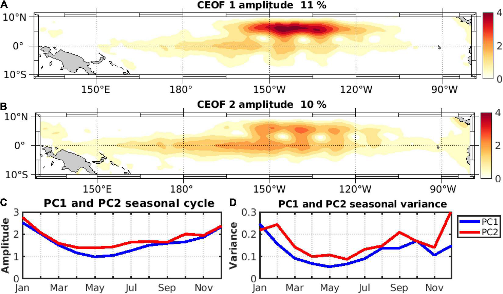
Decomposition into Complex Empirical Orthogonal functions (CEOF) of intraseasonal sea level anomalies (over the period 1993–2018). Spatial patterns of the amplitude of the first CEOF1 (A) and second CEOF2 (B) mode. (C) Seasonal cycle of each mode’s corresponding Principal Component (PC) amplitude, (D) seasonal cycle of each PC amplitude’s monthly variance (PC1 in blue and PC2 in red).
Even though IKWs activity also tends to peak during the onset of El Niño events, in particular during strong Eastern Pacific El Niño events (McPhaden and Yu, 1999; Gushchina and Dewitte, 2012), it is still unclear whether IKWs could also modulate TIWs activity independently of whether or not an El Niño event occurs. In particular, IKWs can reflect as Rossby waves on the density front near 120°W (Mosquera-Vásquez et al., 2014) and trigger coupled Rossby-TIWs (Tanaka and Hibiya, 2019) without invoking changes in background circulation. This represents a strong incentive to investigate a potential consistent IKWs-TIWs interaction. Here, as a preliminary step toward understanding the mechanisms of this interaction at intraseasonal time scales, we analyze almost 30 years of altimetric data to document conjointly both types of waves and their interaction.
Our approach goes beyond the traditional one in that, rather than relating the envelope of TIWs activity to a particular change in the circulation due to an equatorial wave, we attempt to relate specific TIWs and IKWs events. We suggest in particular the existence of a statistically significant mode that couples IKWs and TIWs despite their differences in zonal wavelength and direction of group velocity. The paper is structured as follows: section “Data Sets and Methods” provides an overview of the dataset and methodology. Section “Results” is devoted to the analysis of results of the Complex Empirical Orthogonal Functions (CEOF) and meridional mode decompositions of sea level anomalies, and to the investigation of the forcing mechanism of the IKWs-TIWs coupled mode. In Section “Meridional Eddy Heat Flux Associated With the Intraseasonal Kelvin Waves-Tropical Instability Waves Mode and Implications for the Eastern Equatorial Pacific Heat Budget”, we estimate the contribution of this mode to the non-linear advection in the Eastern Pacific and compare it to the one associated with ENSO time scales. Conclusions are presented in section “Conclusion.”
Data Sets and Methods
Satellite Data
To characterize the oceanic circulation associated with TIWs and IKWs, we use the daily sea level (SLA) and geostrophic currents (U,V) anomalies from the multi-satellite Data Unification and Altimeter Combination System datasets available through the Copernicus Marine Environment Monitoring Service (CMEMS) and the Copernicus Climate Change Service (C3S) (Taburet et al., 2019) at a spatial resolution of 0.25°× 0.25° over the region (10°S–10°N, 130°E–80°W) and the period 1993–2018.
To document the IKWs atmospheric forcing, we calculated the zonal wind stress (τx) considering the drag coefficient formulation of Trenberth et al. (1989) from the 10-m zonal winds from the Fifth Generation ECMWF Atmospheric Reanalysis of the Global Climate (ERA5) (Hersbach et al., 2018) at a 0.25°× 0.25° horizontal resolution over the same region and period than the sea level. Finally, to estimate the meridional oceanic advection associated with the TIWs-IKWs interaction mode, we use the daily sea surface temperatures (SST) from the NOAA 1/4° daily Optimum Interpolation Sea Surface Temperature version 2.1 product (Huang et al., 2020) at a 0.25°× 0.25° resolution over the same period and domain. All data were first linearly detrended. Then, we define the intraseasonal anomalies for all variables as the departure of the instantaneous daily data from the monthly mean following the method by Lin et al. (2000), which is somewhat equivalent to applying a high-pass Lanczos filter with a frequency cut-off at (1/90) days-1 (cf. Dewitte et al., 2011).
Complex Empirical Orthogonal Functions Analyses
Complex Empirical Orthogonal Functions (CEOF) are an efficient tool to disentangle the spatiotemporal characteristics of the intraseasonal variability related to TIWs and KWs as this analysis provides both amplitude and phase information, and is therefore well-suited to capture propagating features (Barnett, 1983; Stein et al., 2011; Boucharel et al., 2013, 2016).
Tropical Instability Waves Amplitude and Indices
To analyze the TIWs characteristics, we use the definition of the TIWs amplitude and index from Boucharel and Jin (2020). We take a simple equally spaced and weighted nodes (positive and negative SLA anomalies) index TIW1. As stated in Boucharel and Jin (2020), the number of nodes and their longitudinal location within the (0°–6°N) band can be chosen arbitrarily. In this study, we chose 6 (SLA) nodes within the (3°N–7°N and 165°–107°W) band that essentially fit the TIWs cusps from the related CEOF mode’s spatial pattern (see section “Satellite Data”).
Where SLA refers to the sea level intraseasonal anomalies. Then, to grasp the TIWs propagation, we define TIW2 similarly to TIW1 except the nodes are now shifted by 90 degrees representing half the TIWs wavelength.
In this paper, we apply this methodology to derive the TIWs activity from the sea level.
Intraseasonal Kelvin Waves Meridional Mode Decomposition
To infer the IKWs contribution to sea level anomalies and interpret the results from the CEOF decomposition, we project the SLA and zonal wind stress anomalies onto the Kelvin/Rossby meridional wave structures in the long wavelength approximation (see Cane and Sarachik, 1976). We assume like in former studies based on satellite sea level (Boulanger and Menkes, 1995; Perigaud and Dewitte, 1996) that the oceanic vertical structure along the equator can be accounted for by just the first baroclinic mode, so that, total sea level (h) and zonal current (u) anomalies can be expressed as a linear combination of meridional mode functions accounting for Kelvin and Rossby waves. This writes as follows:
Where and are the normalized Kelvin and the n-th normalized Rossby waves meridional structures, n denotes the meridional modes being 0 for Kelvin waves and ≥ 1 for the Rossby modes. The rn are the corresponding wave coefficients calculated at each grid point along the equator. The projection of sea level and zonal current anomalies onto the meridional modes is performed between the northern YN and southern limits YS (10°N–10°S in this study). This latitudinal range allows capturing the poleward exponential decrease of Kelvin and Rossby waves and ensuring an approximate orthogonality property between meridional modes.
Where the ψn(y) are the Hermite functions, calculated using a value for phase speed that varies zonally. Its value is set to 3 m/s at 170°W, which corresponds to an average value used in the literature for the first baroclinic mode (Picaut and Sombardier, 1993; Dewitte et al., 1999). We then approximate C(x) as where Zeq is the mean depth of the 20°C isotherm at 170°W and between 2°S and 2°N. Zeq was derived from the global ocean data assimilation system (GODAS, Behringer and Xue, 2004) using the 20°C isotherm depth as a proxy and for the period 1980–2018. The total SLA as well as the SLA reconstructed from the individual CEOF modes are, unless stated otherwise, projected onto the meridional modes functions using the method by Boulanger and Menkes (1995) (see their Appendix B), which does not require the knowledge of zonal current anomalies and is comparable to assuming that Rossby wave coefficients are negligible from a certain rank (see also Perigaud and Dewitte, 1996).
The zonal wind stress is also projected onto the theoretical meridional mode structures of the first baroclinic mode, and its contribution to the Kelvin wave is inferred from the following formula: τx (x, y, t) = Fo (x, t) Rn (y), and
Where h, u and τx come from observations described in section” Satellite Data.”
Results
Complex Empirical Orthogonal Functions Analysis of Sea Level Anomalies
Results from the CEOF decomposition of the sea level intraseasonal anomalies are presented in Figure 1. The first two modes grasp 21% of the explained variance of the total sea level anomalies over the spatial domain shown in Figure 1, almost equally distributed. Since higher-order modes explain individually less than 5.4% of the variance, in the following we focused on the first two modes only. The first mode (CEOF1), characterized by a strong amplitude between 3–7°N and 120–165°W (Figure 1A), mostly captures the variability associated with TIWs (with an explained variance of 11%) although a relative maximum amplitude is also observed along the equator reminiscent of IKWs contribution to sea level anomalies. The real part of the spatial CEOF pattern (Supplementary Figure 2A) exhibits TIWs cusps similarly positioned as in Xue et al. (2020). The decreasing phase from east to west in this region shown on the CEOF spatial phase pattern (Supplementary Figure 3A) characterizes the TIWs westward propagation. The second mode (CEOF2), which explains a similar amount of variance, exhibits a comparable phase (Supplementary Figure 3B) and amplitude pattern although the amplitude along the equator is about twice as large as that of the first mode while the amplitude of the TIWs cups is smaller. Note also the exact same location of the TIWs cups but with opposite value of amplitude of the real part between CEOF1 and CEOF2 (Supplementary Figure 2), which results from the orthogonality of the two modes’s patterns and suggests that they capture the same sequence of TIWs propagations. Their summed-up contribution explains 42% of the variance of the total sea level anomalies over the region (2°S–2°N, 170–120°W). The summed-up contribution from CEOF1 and CEOF2 over the TIWs active region (3–7°N and 165–107°W) was also found to be highly correlated with both TIWs index and TIWs amplitude from Boucharel and Jin (2020) (r = 0.5 and 0.7 respectively, not shown) which all together indicates that CEOF1 + 2 capture most of TIWs variability. In the equatorial band, the zonally elongated pattern symmetrical around the equator, more pronounced for CEOF2 than for CEOF1, is indicative of the IKWs activity and suggests that the two modes capture the non-linear interaction between IKWs and TIWs. The phase patterns of the two modes along the equator (Supplementary Figure 3) confirm the eastward propagation at a phase speed estimated to 2.6 m/s consistent with former studies based on altimetry data (Cravatte et al., 2003; Dewitte et al., 2003). Their projections onto the Kelvin wave structure indicate that CEOF2 explains 24% of the variance of the Kelvin wave contribution to the full sea level anomalies average over (2°S–2°N, 170–120°W) while CEOF1 only explains 12.9% (see Table 1). The maximum correlation between sea level anomalies reconstructed from CEOF1 and CEOF2 is reached (r = 0.3 between 2°S–2°N and 170–120°W) at a positive lag of 14 days [Principal Component (PC) 1 lags PC2], corresponding to about a quarter of the main period of IKWs, which confirms that the two modes capture the same sequences of IKWs. In order to diagnose the seasonality of the PC timeseries, their climatology and climatological variance are shown in Figures 1C,D, respectively, which indicates they both have a peak amplitude during the boreal summer and fall, consistent with the expectation that they grasp the same seasonally synchronized interaction mode between IKWs and TIWs. Lastly, the correlation between the 3-month running variance of PC1 and PC2 reaches 0.84 which confirms that the two modes grasp the same physical mode of interaction between IKWs and TIWs.
TABLE 1
| SLA reconstructed from | TIWs amplitude | TIWs amplitude without the La Niña events | SLA | SLA averaged without the La Niña events |
| CEOF 1 | 21.7% | 20.1% | 12.9% | 3.0% |
| CEOF 2 | 27.2% | 27.9% | 24.0% | 15.0% |
| CEOF 1 + 2 | 31.6% | 33.1% | 42.0% | 26.0% |
Explained variance (%) of SLA and TIWs amplitude explained by the SLA reconstructed from CEOF 1, CEOF2 and CEOF1 + 2.
This table shows the explained variance of the sea level reconstructed from CEOF 1, CEOF 2 and CEOF 1 + 2 and averaged at the equator (2°S–2°N, 170–120°W) and the TIWs amplitude derived from the TIWs index calculated using sea level anomaly and following the methodology by Boucharel and Jin (2020). The explained variance is also compared without La Niña periods defined as the period when the C index is less than −0.5°C.
Composite Analysis
In order to document further the relationship between IKWs and TIWs, we perform a lead-lag composite analysis of strong events identified from the SLA timeseries reconstructed from CEOF2 and averaged in the equatorial region (2°S–2°N, 180–80°W). This choice is motivated by the fact that (i) CEOF2 grasps twice as much variance along the equator (see Table 1) and therefore can be interpreted as the portion of TIWs variability that relates to IKWs, and (ii) PC2 leads PC1 slightly (by ∼15 days). 25 downwelling and 28 upwelling events are identified for which the equatorial SLA reconstructed from CEOF2 is above or below 2 standard deviations, respectively (Figure 2A). Figure 2 shows the composite evolution of the dominant EOF mode of equatorial zonal wind stress intraseasonal anomalies in the equatorial band (Figure 2B, see also its spatial pattern and temporal evolution in Supplementary Figures 4, 5 respectively), the equatorial Kelvin wave contribution to sea level anomalies, and the reconstructed sea level anomalies from CEOF2 (Figures 2C). In particular, Figure 2B,C indicate that the positive equatorial SLA events in the central Pacific characterize strong downwelling IKWs triggered by westerly wind bursts that occurred on average ∼10 days prior in the Western Pacific. These westerly wind anomalies spread toward the central-western Pacific and maintain the eastward propagation of IKWs, which take approximately 30 days to cross the entire basin, consistently with the IKWs phase speed. Similar composite patterns but with a reverse sign are observed during upwelling events sparked by easterly wind bursts (Supplementary Figure 6). Interestingly, most of the events used to conduct this lag-composite analysis can also be found in the upwelling IKWs either preceding or following the composite downwelling IKWs presented in Figure 2. This means that the basin scale CEOF analysis, which inherently encompasses most IKWs propagation features into a single mode does not allow disentangling quantitatively the IKWs phases but rather represents the succession of upwelling and downwelling pulses as an integrated pattern of IKWs variability. This is why we observe active TIWs in the northeastern tropical Pacific throughout the entire IKWs propagation cycle across the basin (Figure 2C and Supplementary Figure 6B). Their presence in the eastern Pacific, whereas the IKWs has yet to reach the area, has likely been triggered by the preceding IKWs (∼60 days prior).
FIGURE 2
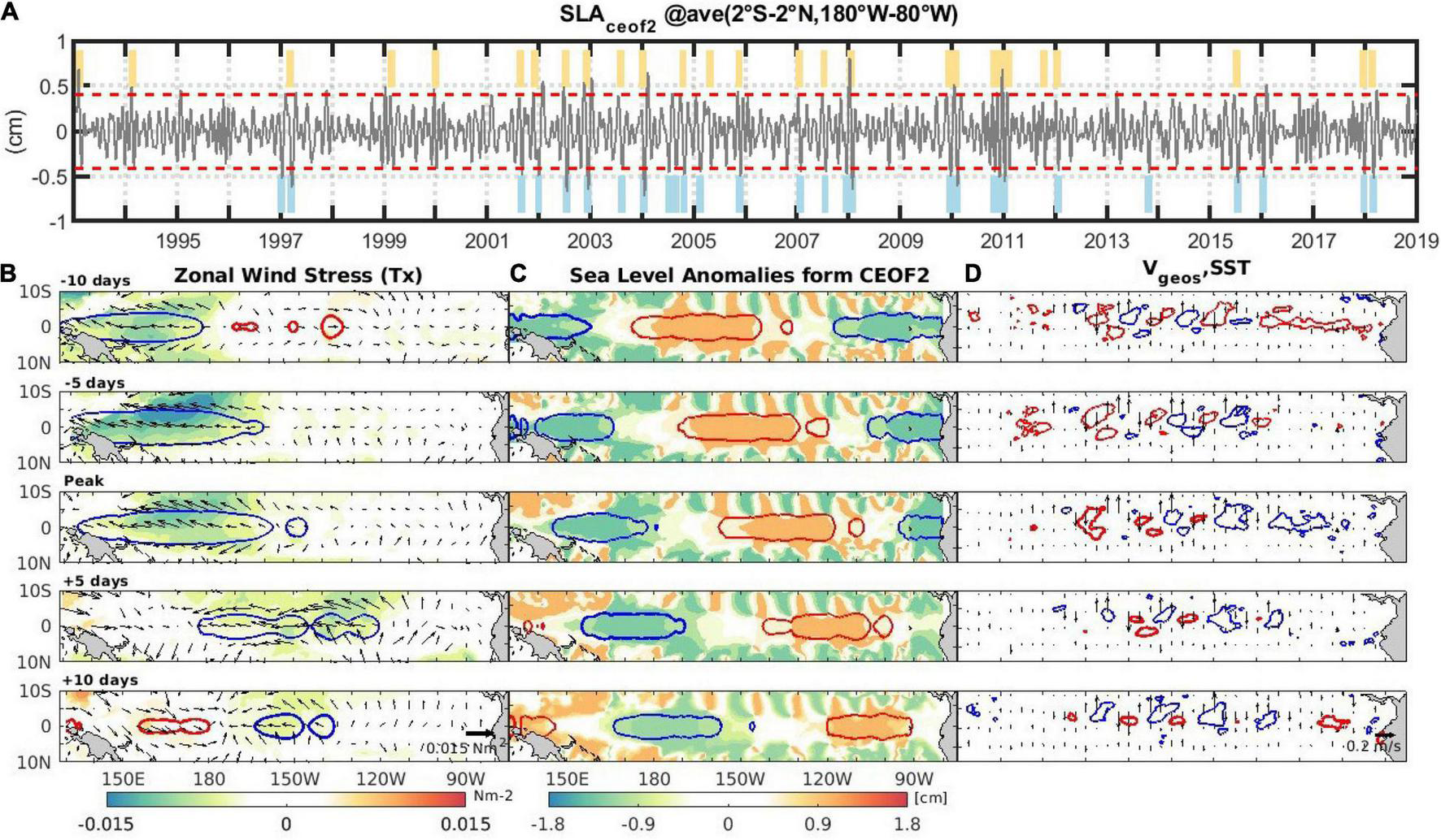
(A) SLA reconstructed from CEOF2 and averaged in the region (2°S–2°N, 180°W–80°W). SLA events above (below) 2 standard deviations are highlighted in yellow (blue). (B, left panels) Composites of the corresponding intraseasonal wind stress anomalies (in Nm– 2) reconstructed from the first EOF mode at different leads/lags (centered, i.e., lag 0, at the SLA peak from A). The colored contours represent the intraseasonal zonal wind stress anomalies projected onto the theoretical Kelvin wave meridional structure; blue (red) contours correspond to -0.002 Nm– 2 (+ 0.002 Nm– 2). (C, middle panels) Composites (shading in cm) of SLA reconstructed from CEOF2 at different leads/lags (in days) indicated on the top left of the leftmost panels and centered (i.e., lag 0) during the strong positive intraseasonal equatorial sea level anomalies events identified in (A) (i.e., the IKWs downwelling phases). The colored contours represent the intraseasonal SLA projected onto the theoretical Kelvin wave meridional structure; blue (red) contours are for values of -0.5 (+ 0.5) cm. (D, right panels) Composites of meridional geostrophic velocity anomalies (arrows), and SST anomalies [red (blue) contours corresponds to 0.2 (-0.2)°C].
Although the CEOF analysis is not designed to grasp asymmetry in the variability, still, we can observe that the amplitude of the CEOF2 SLA as well as the SST and meridional geostrophic velocity anomalies composite (superimposed on Figure 2D and Supplementary Figure 6C) in the region of TIWs activity is larger during the upwelling than the downwelling IKWs propagation cycle. In order to further quantify such asymmetrical response in TIWs amplitude to the IKWs phase, we present in Figure 3, a bar plot between total SLA averaged in the equatorial region (2°S–2°N, 150–80°W) and TIWs amplitude calculated from SLA using Boucharel and Jin’s (2020) method for the strong upwelling and downwelling events identified previously. Figure 3 indicates that upwelling IKWs tend to promote a larger TIWs amplitude than downwelling IKWs by ∼15%. Note that this is significant at the ∼90% level based on a Student’s t-test. This is consistent with the theoretical and modeling study by HT16 who also evidenced an asymmetry in the amplitude of the TIWs activity between the passage of upwelling and downwelling IKWs, although in their case the TIWs response is somewhat stronger (in their experiments, the TIWs kinetic energy is decreased (increased) by 38% (42%) for downwelling (upwelling) IKWs compared to the background control). In addition, in their idealized setting, HT16 estimated a ∼60 days lagged TIWs response to the passage of IKWs, while we find a faster response (∼10–15 days). These differences can be attributed to the distinct methodological approaches between the two studies. In particular, while we diagnose the lag in SLA amplitude between the equatorial and TIWs regions, HT16 use the rate of volume averaged TIWs kinetic energy, which has a longer time scale adjustment due to its quadratic formulation and may encompass the contribution of high-order baroclinic modes due to the depth integration. In addition, unlike in HT16’s idealized settings, the different Kelvin waves phases are not well differentiated in our CEOF observational analysis as most of the time they form a sequence a 2–3 pulses of waves (i.e., wave trains). So, it is expected that the lagged relationship between TIWs and IKWs in the data differs from that in their modeling study, because of the cumulative effect of consecutive IKWs on TIWs activity.
FIGURE 3
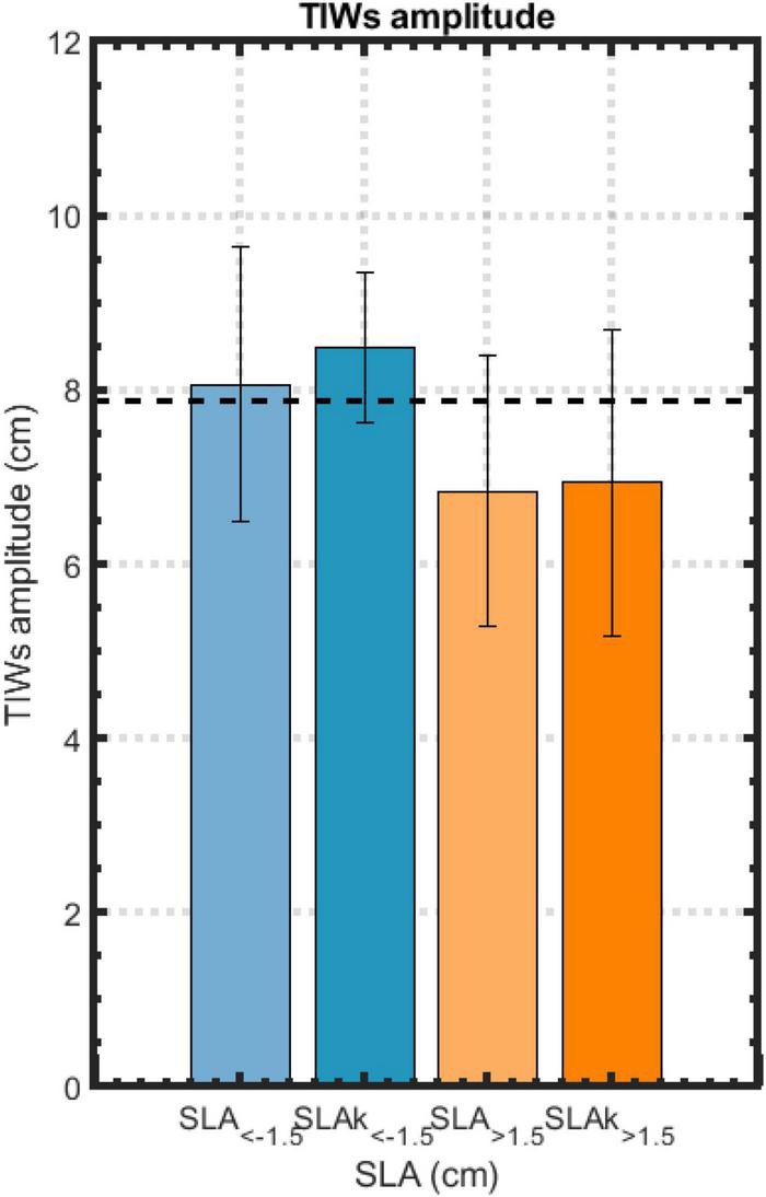
Mean TIWs amplitude (calculated using the method described in Boucharel and Jin, 2020, applied on SLA reconstructed from CEOF1 + 2) during upwelling (blue) and downwelling (orange) events. Upwelling (Downwelling) events correspond to events identified in Figure 2A restricted to when the total sea level anomalies averaged in the region (2°S–2°N, 150–80°W) are below −1.5 cm (above +1.5 cm). Similarly, the dark blue and orange bars represent the average TIWs amplitude for upwelling (downwelling) events when the total sea level anomalies projected on the Kelvin wave mode (SLAk) are below −1.5 cm (above +1.5 cm). The error bars represent ± 1 standard deviation of TIWs amplitude amongst the retained events. The dashed black horizontal line indicates the annual mean of TIWs amplitude calculated from the method by Boucharel and Jin (2020) applied on the total sea level.
The composite patterns of sea level, SST and meridional geostrophic velocity anomalies at the peak of the passing IKWs (Figure 4) in the region of TIWs activity not only confirms the somewhat asymmetrical response in the TIWs amplitude but also showcase an in-phase signal between temperature and meridional currents anomalies likely leading to a TIWs-induced meridional heat flux convergence (Xue et al., 2020). This now raises the question of the contribution of these coupled IKWs-TIWs individual events to the Cold Tongue heat budget and in particular, to which extent they compare to the strong TIWs-induced non-linear dynamical heating evidenced at seasonal and interannual time scales in previous studies (e.g., Wang and McPhaden, 1999; Menkes et al., 2006; An, 2008; Xue et al., 2020, 2021).
FIGURE 4

Composites of SLA, meridional geostrophic velocity anomalies (arrows) and SST anomalies [red (blue) contours corresponds to 0.2 (-0.2)°C] at the peak of a strong events in sea level anomalies (i.e., IKW) along the equator (cf. Figure 2A) [(A) for downwelling, (B) for upwelling].
Meridional Eddy Heat Flux Associated With the Intraseasonal Kelvin Waves-Tropical Instability Waves Mode and Implications for the Eastern Equatorial Pacific Heat Budget
While most focus has been drawn to TIWs-induced heat flux convergence associated with interannual fluctuations in the background state (i.e., ENSO) in earlier studies, our results call for the evaluation the TIWs-induced non-linear dynamical heating (NDH) at intraseasonal time scales. The seasonally varying TIWs has been shown to warm the equatorial cold tongue through meridional heat advection (Wang and McPhaden, 1999). Similarly, many studies have highlighted the TIWs effect at interannual time scales as a potential source for ENSO asymmetry (An, 2008; Boucharel and Jin, 2020; Xue et al., 2020, 2021) due to the rectified effect of anomalous temperature transport by anomalous currents referred to as oceanic eddy heat flux (e.g., Baturin and Niiler, 1997; Menkes et al., 2006; Jochum and Murtugudde, 2006; Jochum et al., 2007, 2008; Graham, 2014; Xue et al., 2020). In this section, we estimate the eddy heat flux spatial derivative composite of the specific events that correspond to periods of strong activity of the IKWs-TIWs interaction mode. This allows diagnosing the NDH of the eastern equatorial Pacific triggered by the passage of strong downwelling and upwelling IKWs. The intraseasonal NDH is approximated here by NDHTIWs = v′∂yT′ following Xue et al. (2020).
Figure 5 shows the TIWs-induced intraseasonal meridional NDH composite associated with the upwelling (a) and downwelling (b) phase of the IKWs-TIWs interaction mode. They both exhibit a warming pattern located just north of the equator along with a cooling pattern centered around 4°N indicating a rather similar TIWs-induced entrainment of warm equatorial water into the Cold Tongue region between the two IKWs phases. As an integrated measure of the warming effect of the IKWs-TIWs interaction mode on the eastern equatorial Pacific, we present in Figure 5C the intraseasonal NDH longitudinally averaged between 150°W and 110°W (the same region as in Xue et al., 2020). It confirms the rather similar magnitude of NDHTIWs (∼0.8°C/month) during both the downwelling and upwelling IKWs phases, albeit slightly stronger during upwelling events due to the stronger TIWs activity (Figure 3). Note however that there is a significant spread (dotted line in Figure 5C) amongst the individual events, which reflects a large diversity in the response of NDHTIWs to individual IKWs or IKWs trains. The spread tends to be larger among the upwelling events along the equator (see dashed turquoise thin line in Figure 5C). What is also noticeable from Figure 5C is that NDHTIWs falls within the range of warming induced by the interannual eddy heat flux convergence as indicated by the latitudinal profiles of the El Niño and La Niña meridional NDH composites during their developing phase (i.e., July–November average) over the same period (1993–2018). Note that the latter is mostly induced by the prolonged La Niña event (1998–2001) that followed the strong Eastern Pacific El Niño of 1997/98 (not shown). Although both triggered by TIWs-induced NDH, the Cold Tongue warming presumably originates from different dynamical mechanisms.
FIGURE 5
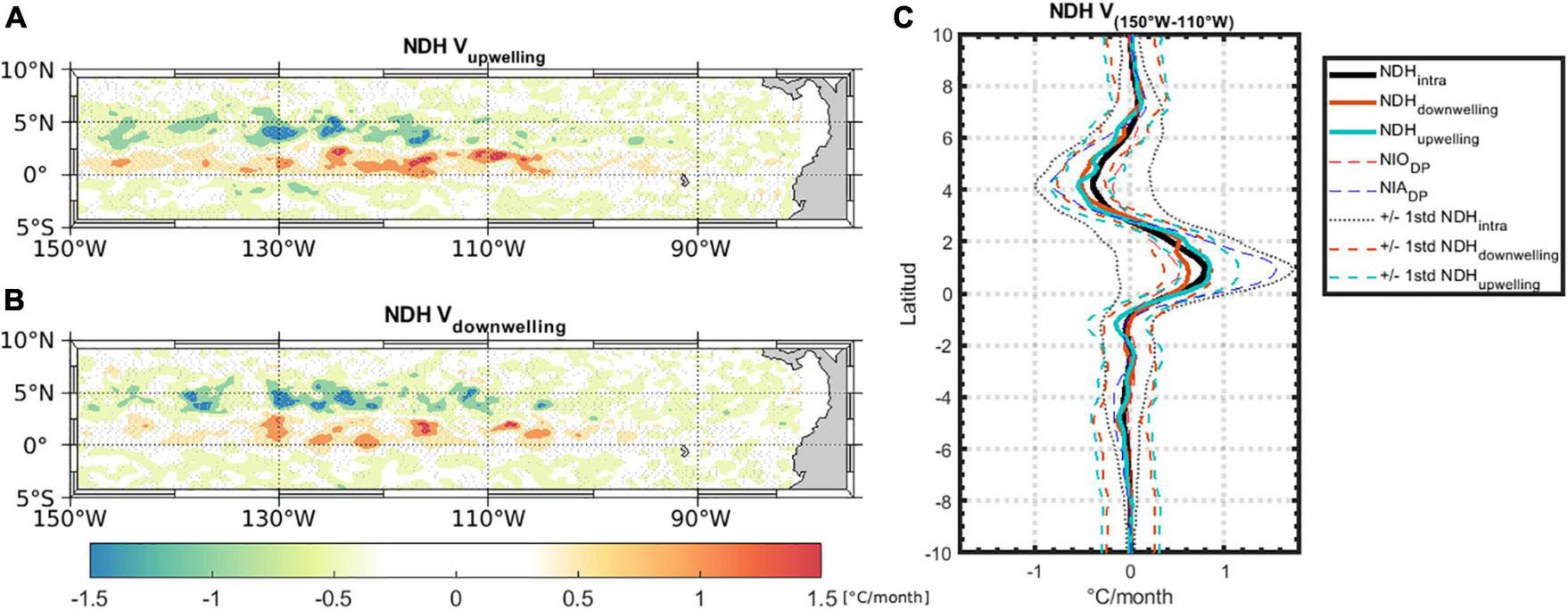
Composites of meridional components of intraseasonal Non-linear Dynamical Heating (NDH) during upwelling (A) and downwelling (B) IKWs events identified in Figure 2A. (C) Longitudinal average (between 150 and 110°W) of intraseasonal NDH annual mean (thick black line), IKWs upwelling phases (thick turquoise line), IKWs downwelling phases (thick brown line), interannual El Niño (dashed red line) and La Niña (dashed blue line) developing phase (July–November) NDH composite. The thin black (orange/turquoise) dashed lines indicate ± 1 standard deviation of the total intraseasonal NDH (amongst the downwelling/upwelling events). Units are °C/month.
Conclusion
In this study, we have analyzed 26 years of altimetric data to document the interaction between TIWs and IKWs, observing that TIWs activity is only weakly linearly related to ENSO. Our statistical (complex EOF) analysis evidences a coupling between these equatorial waves contained in the first two dominant modes of the intraseasonal SLA decomposition that explain together 21% of the total variance. In detail, the first mode (11%) tends to dominantly capture the TIWs activity and is correlated to typical TIWs variance indices, while the second mode (10%) leading the first mode by ∼10 days, exhibits a comparable loading in the equatorial and TIWs region, best accounting for the interaction between IKWs and TIWs. The two modes have also similar seasonal modulation with a peak activity in the austral summer like ENSO. However, their interannual modulation is not linearly related to ENSO with in particular a peak activity taking place predominantly during non-El Niño or non-La Niña years (43 and 51% for modes 1 and 2, respectively). This is consistent with the interpretation that the intraseasonal Kelvin wave has the capacity to modulate the background conditions over which TIWs can grow, and that this does not necessarily require variations in mean conditions at low-frequency (e.g., ENSO). HT16 showed in particular that IKWs can disrupt the zonal currents background and thus the TIWs kinetic energy balance through lateral shear production, despite the fact TIWs and IKWs time scales are intertwined, making unclear to which extent individual IKWs can produce changes in background conditions sufficiently fast for this barotropic instability to develop. Our results are thus consistent with the experimental findings of HT16 suggesting that the statistical modes documented in this study could be interpreted as resulting from such a mechanism, although the distinct methodological approaches between the two studies lead to differences in the lagged and asymmetric response of the TIWs amplitude to the passage of different phases of IKWs. However, further investigations based on a regional ocean model are needed to confirm if the mechanism proposed by HT16 applies to observed events accounted for by the statistical modes documented here. Events taking place during “normal” years (i.e., non-ENSO) represent case studies to consider for our future investigation in order to rule out the influence of variability at time scales larger than that associated with episode of IKWs. For instance, the years 2003 and 2013 that correspond to “neutral” years in terms of interannual variability showcase a succession of events that are well accounted for by the statistical modes (Figure 6). Figure 6 indicates in particular that TIWs (accounted for by CEOF1 for the June 2003 event and CEOF2 for the August 2003 and October 2013 events) start growing as an upwelling IKWs propagates across the central Pacific, suggesting that IKWs-induced modification in the circulation is sufficiently “slow” for the instability to grow despite the closeness of peak frequencies between the two waves. It is interesting to note that TIWs activity is increased (reduced) during the passage of upwelling (downwelling) IKWs, even though our analysis makes difficult to isolate the impact of individual IKWs events. Although this TIWs modulation occurs almost instantaneously, this is consistent with the asymmetric TIWs amplitude response to the passage of IKWs found in HT16 (yet with a weaker response). Note that previous studies have identified from observations two distinct modes of TIWs in the eastern equatorial Pacific with periods near 33 and 17 days, and commonly referred to as the Rossby and Yanai modes, respectively (Lyman et al., 2007; Cai et al., 2020). Here the CEOF2 mode has a dominant frequency at ∼(1/57) days-1, suggesting that it may encapsulate the rectified effect of instability processes associated with these Rossby and Yanai modes. This needs further investigation based on the experimentation with a high-resolution ocean model, which is our current plan.
FIGURE 6
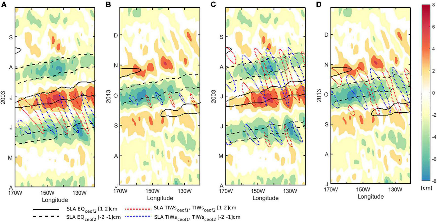
IKWs and TIWs evolution during two periods (A,C. April-September 2003 and B,D. July–December 2013): Hovmoller of total SLA (color) at the equator (2°S–2°N), SLA reconstructed from CEOF2 projected onto the Kelvin mode (upwelling/downwelling in dashed/continuous black contours, at the equator) and SLA reconstructed from CEOF 1 (A,B) and from CEOF2 (C,D) in the TIWs region (3°N–7°N) [dashed blue (red) lines for negative (positive) SLA].
Publisher’s Note
All claims expressed in this article are solely those of the authors and do not necessarily represent those of their affiliated organizations, or those of the publisher, the editors and the reviewers. Any product that may be evaluated in this article, or claim that may be made by its manufacturer, is not guaranteed or endorsed by the publisher.
Statements
Data availability statement
The original contributions presented in the study are included in the article/Supplementary Material, further inquiries can be directed to the corresponding author/s.
Author contributions
JB and BD: conceptualization. ME-F: methodology, data curation, and writing—original draft preparation. All authors have discussed the results and contributed to writing the manuscript.
Funding
BD acknowledges support from ANID (Concurso de Fortalecimiento al Desarrollo Científico de Centros Regionales 2020-R20F0008-CEAZA, Grant 1190276 and COPAS COASTAL FB210021) and ANR (Grant ANR-18-CE01-0012). JB was funded by the French Agence Nationale de la Recherche project Make Our Planet Great Again (MOPGA) “Trocodyn” (ANR-17-MPGA-0018) and GE was funded by the Région Occitanie.
Conflict of interest
The authors declare that the research was conducted in the absence of any commercial or financial relationships that could be construed as a potential conflict of interest.
Supplementary material
The Supplementary Material for this article can be found online at: https://www.frontiersin.org/articles/10.3389/fmars.2022.788908/full#supplementary-material
References
1
Allen M. R. Lawrence S. P. Murray M. J. Mutlow C. T. Stockdale T. N. Llewellyn-Jones D. T. et al (1995). Control of tropical instability waves in the Pacific.Geophys. Res. Lett.222581–2584. 10.1029/95GL02653
2
An S.-I. (2008). Interannual Variations of the Tropical Ocean Instability Wave and ENSO.J. Clim.213680–3686. 10.1175/2008JCLI1701.1
3
Barnett T. P. (1983). Interaction of the Monsoon and Pacific Trade Wind System at Interannual Time Scales Part I: The Equatorial Zone.Monthly Weather Rev.111756–773. 10.1175/1520-04931983111<0756:IOTMAP<2.0.CO;2
4
Baturin N. G. Niiler P. P. (1997). Effects of instability waves in the mixed layer of the equatorial Pacific.J. Geophys. Res.10227771–27793. 10.1029/97JC02455
5
Behringer D. Xue Y. (2004). “Evaluation of the global ocean data assimilation system at NCEP: The Pacific Ocean,” in AMS 84th Annual Meeting, (Seattle, WA: AMS), 7.
6
Benestad R. E. Sutton R. T. Allen M. R. Anderson D. L. T. (2001). The influence of subseasonal wind variability on tropical instability waves in the Pacific.Geophys. Res. Lett.282041–2044. 10.1029/2000GL012563
7
Boucharel J. Jin F.-F. (2020). A simple theory for the modulation of tropical instability waves by ENSO and the annual cycle.Tellus Dynam. Meteorol. Oceanogr.721–14. 10.1080/16000870.2019.1700087
8
Boucharel J. Jin F.-F. England M. H. Dewitte B. Lin I. I. Huang H.-C. et al (2016). Influence of Oceanic Intraseasonal Kelvin Waves on Eastern Pacific Hurricane Activity.J. Clim.297941–7955. 10.1175/JCLI-D-16-0112.1
9
Boucharel J. Timmermann A. Jin F.-F. (2013). Zonal phase propagation of ENSO sea surface temperature anomalies: Revisited.Geophys. Res. Lett.404048–4053. 10.1002/grl.50685
10
Boulanger J.-P. Menkes C. (1995). Propagation and reflection of long equatorial waves in the Pacific Ocean during the 1992–1993 El Niño.J. Geophys. Res.100:25041. 10.1029/95JC02956
11
Cai W. McPhaden M. J. Grimm A. Rodrigues R. R. Taschetto A. S. (2020). Climate impacts of the El Niño–Southern Oscillation on South America.Nat. Rev. Earth Environ.1215–231. 10.1038/s43017-020-0040-3
12
Cane M. Sarachik E. (1976). Forced Baroclinic Ocean Motions. 1. Linear Equatorial Unbounded Case.J. Mar. Res.34629–665.
13
Capotondi A. Deser C. Phillips A. S. Okumura Y. Larson S. M. (2020). ENSO and Pacific Decadal Variability in the Community Earth System Model Version 2.J. Adv. Model. Earth Syst.12:2019MS002022. 10.1029/2019MS002022
14
Chelton D. B. Esbensen S. K. Schlax M. G. Thum N. Freilich M. et al (2001). Observations of Coupling between Surface Wind Stress and Sea Surface Temperature in the Eastern Tropical Pacific.J. Clim.141479–1498. 10.1175/1520-04422001014<1479:OOCBSW<2.0.CO;2
15
Choi J. An S.-I. Dewitte B. Hsieh W. W. (2009). Interactive Feedback between the Tropical Pacific Decadal Oscillation and ENSO in a Coupled General Circulation Model.J. Clim.226597–6611. 10.1175/2009JCLI2782.1
16
Choi J. An S.-I. Kug J.-S. Yeh S.-W. (2011). The role of mean state on changes in El Niño’s flavor.Clim. Dyn.371205–1215. 10.1007/s00382-010-0912-1
17
Choi J. An S.-I. Yeh S.-W. Yu J.-Y. (2013). ENSO-Like and ENSO-Induced Tropical Paci?c Decadal Variability in CGCMs.J. Clim.26:17.
18
Cox M. D. (1980). Generation and Propagation of 30-Day Waves in a Numerical Model of the Pacific.J. Physical Oceanogr.101168–1186. 10.1175/1520-04851980010<1168:GAPODW<2.0.CO;2
19
Cravatte S. Eldin G. Picaut J. (2003). Second and first baroclinic Kelvin modes in the equatorial Pacific at intraseasonal timescales.J. Geophys. Res.10822–21. 10.1029/2002JC001511
20
Delpech A. Cravatte S. Marin F. Ménesguen C. Morel Y. (2020). Deep Eddy Kinetic Energy in the Tropical Pacific From Lagrangian Floats.J. Geophys. Res.125:23. 10.1029/2020JC016313
21
Dewitte B. Illig S. Parent L. duPenhoat Y. Gourdeau L. Verron J. (2003). Tropical Pacific baroclinic mode contribution and associated long waves for the 1994-1999 period from an assimilation experiment with altimetric data.J. Geophys. Res.1083121–3138. 10.1029/2002JC001362
22
Dewitte B. Illig S. Renault L. Goubanova K. Takahashi K. Gushchina D. et al (2011). Modes of covariability between sea surface temperature and wind stress intraseasonal anomalies along the coast of Peru from satellite observations (2000–2008).J. Geophys. Res.116:C04028. 10.1029/2010JC006495
23
Dewitte B. Reverdin G. Maes C. (1999). Vertical Structure of an OGCM Simulation of the Equatorial Paci?c Ocean in 1985–94.J. Physical Oceanogr.29:29.
24
Dutrieux P. Menkes C. E. Vialard J. Flament P. Blanke B. (2008). Lagrangian Study of Tropical Instability Vortices in the Atlantic.J. Physical Oceanogr.38:18.
25
Evans W. Strutton P. G. Chavez F. P. (2009). Impact of tropical instability waves on nutrient and chlorophyll distributions in the equatorial Pacific.Deep Sea Res. Part I Oceanogr. Res. Pap.56178–188. 10.1016/j.dsr.2008.08.008
26
Flament P. J. Kennan S. C. Knox R. A. Niiler P. P. Bernstein R. L. (1996). The three-dimensional structure of an upper ocean vortex in the tropical Pacific Ocean.Nature383610–613. 10.1038/383610a0
27
Giese B. S. Harrison D. E. (1991). Eastern equatorial Pacific response to three composite westerly wind types.J. Geophys. Res.96:3239. 10.1029/90JC01861
28
Graham T. (2014). The importance of eddy permitting model resolution for simulation of the heat budget of tropical instability waves.Ocean Model.7921–32. 10.1016/j.ocemod.2014.04.005
29
Gushchina D. Dewitte B. (2012). Intraseasonal Tropical Atmospheric Variability Associated with the Two Flavors of El Niño.Monthly Weather Rev.1403669–3681. 10.1175/MWR-D-11-00267.1
30
Harrison D. E. Giese B. S. (1988). Remote westerly wind forcing of the eastern equatorial Pacific; Some model results.Geophys. Res. Lett.15804–807. 10.1029/GL015i008p00804
31
Hashizume H. Xie S.-P. Liu W. T. Takeuchi K. (2001). Local and remote atmospheric response to tropical instability waves: A global view from space.J. Geophys. Res.10610173–10185. 10.1029/2000JD900684
32
Hersbach H. Bell B. Berrisford P. et al (2018). ERA5 hourly data on pressure levels from 1979 to present. Available online at: https://cds.climate.copernicus.eu/cdsapp#!/dataset/reanalysis-era5-pressure-levels?tab=overview(accessed January 1, 2020).
33
Holmes R. M. Thomas L. N. (2015). The Modulation of Equatorial Turbulence by Tropical Instability Waves in a Regional Ocean Model.J. Physical Oceanogr.451155–1173. 10.1175/JPO-D-14-0209.1
34
Holmes R. M. Thomas L. N. (2016). Modulation of Tropical Instability Wave Intensity by Equatorial Kelvin Waves.J. Physical Oceanogr.462623–2643. 10.1175/JPO-D-16-0064.1
35
Hsin Y.-C. Qiu B. (2012). The impact of Eastern-Pacific versus Central-Pacific El Niños on the North Equatorial Countercurrent in the Pacific Ocean.J. Geophys. Res.117:2012JC008362. 10.1029/2012JC008362
36
Huang B. Liu C. Banzon V. F. Freeman E. Graham G. Hankins B. et al (2020). NOAA 0.25-degree Daily Optimum Interpolation Sea Surface Temperature (OISST), Version 2.1.NOAA Natl. Centers Environ. Informat.2020:T57. 10.25921/RE9P-PT57
37
Imada Y. Kimoto M. (2012). Parameterization of Tropical Instability Waves and Examination of Their Impact on ENSO Characteristics.J. Clim.254568–4581. 10.1175/JCLI-D-11-00233.1
38
Inoue R. Lien R.-C. Moum J. N. (2012). Modulation of equatorial turbulence by a tropical instability wave: Equatorial Turbulence Modulated by a TIW.J. Geophys. Res.117:2011JC007767. 10.1029/2011JC007767
39
Izumo T. (2005). The equatorial undercurrent, meridional overturning circulation, and their roles in mass and heat exchanges during El Niño events in the tropical Pacific ocean.Ocean Dynam.55110–123. 10.1007/s10236-005-0115-1
40
Izumo T. Picaut J. Blanke B. (2002). Tropical pathways, equatorial undercurrent variability and the 1998 La Niña.Geophys. Res. Lett.2937–31. 10.1029/2002GL015073
41
Jing Z. Wu L. Wu D. Qiu B. (2014). Enhanced 2-h–8-day Oscillations Associated with Tropical Instability Waves.J. Physic. Oceanogr.441908–1918. 10.1175/JPO-D-13-0189.1
42
Jochum M. Murtugudde R. (2006). Temperature Advection by Tropical Instability Waves.J. Physic. Oceanogr.36592–605. 10.1175/JPO2870.1
43
Jochum M. Cronin M. F. Kessler W. S. Shea D. (2007). Observed horizontal temperature advection by tropical instability waves.Geophys. Res. Lett.34:2007GL029416. 10.1029/2007GL029416
44
Jochum M. Danabasoglu G. Holland M. Kwon Y.-O. Large W. G. (2008). Ocean viscosity and climate.J. Geophys. Res.113:C06017. 10.1029/2007JC004515
45
Kennan S. C. Flament P. J. (2000). Observations of a Tropical Instability Vortex *.J. Phys. Oceanogr.302277–2301. 10.1175/1520-04852000030<2277:OOATIV<2.0.CO;2
46
Lawrence S. P. Allen M. R. Anderson D. L. T. Llewellyn-Jones D. T. (1998). Effects of subsurface ocean dynamics on instability waves in the tropical Pacific.J. Geophys. Res.10318649–18663. 10.1029/98JC01684
47
Lawrence S. P. Angell J. P. (2000). Evidence for Rossby wave control of tropical instability waves in the Pacific Ocean.Geophys. Res. Lett.272257–2260. 10.1029/1999GL002363
48
Lee T. Lagerloef G. Gierach M. M. Kao H.-Y. Yueh S. Dohan K. (2012). Aquarius reveals salinity structure of tropical instability waves.Geophys. Res. Lett.39:2012GL052232. 10.1029/2012GL052232
49
Legeckis R. (1977). Long waves in the eastern equatorial Pacific Ocean: A view from a geostationary satellite.Science1971179–1181. 10.1126/science.197.4309.1179
50
Legeckis R. Brown C. W. Bonjean F. Johnson E. S. (2004). The influence of tropical instability waves on phytoplankton blooms in the wake of the Marquesas Islands during 1998 and on the currents observed during the drift of the Kon-Tiki in 1947.Geophys. Res. Lett.31:2004GL021637. 10.1029/2004GL021637
51
Lien R.-C. D’Asaro E. A. Menkes C. E. (2008). Modulation of equatorial turbulence by tropical instability waves.Geophys. Res. Lett.35:L24607. 10.1029/2008GL035860
52
Lin J. W.-B. Neelin J. D. Zeng N. (2000). Maintenance of Tropical Intraseasonal Variability: Impact of Evaporation–Wind Feedback and Midlatitude Storms.J. Atmospheric Sci.57:31.
53
Liu C. Köhl A. Liu Z. Wang F. Stammer D. (2016). Deep-reaching thermocline mixing in the equatorial pacific cold tongue.Nat. Commun.7:11576. 10.1038/ncomms11576
54
Luther D. S. Johnson E. S. (1990). Eddy Energetics in the Upper Equatorial Pacific during the Hawaii-to-Tahiti Shuttle Experiment.J. Physic. Oceanogr.20913–944. 10.1175/1520-04851990020<0913:EEITUE<2.0.CO;2
55
Lyman J. M. Chelton D. B. deSzoeke R. A. Samelson R. M. (2005). Tropical Instability Waves as a Resonance between Equatorial Rossby Waves*.J. Physic. Oceanogr.35232–254. 10.1175/JPO-2668.1
56
Lyman J. M. Johnson G. C. Kessler W. S. (2007). Distinct 17- and 33-Day Tropical Instability Waves in Subsurface Observations*.J. Physic. Oceanogr.37855–872. 10.1175/JPO3023.1
57
McPhaden M. J. (1996). Monthly period oscillations in the Pacific North Equatorial Countercurrent.J. Geophys. Res.1016337–6359. 10.1029/95JC03620
58
McPhaden M. J. Yu X. (1999). Equatorial waves and the 1997-98 El Niño.Geophys. Res. Lett.262961–2964. 10.1029/1999GL004901
59
Menkes C. E. (2002). A whirling ecosystem in the equatorial Atlantic.Geophys. Res. Lett.29:1553. 10.1029/2001GL014576
60
Menkes C. E. Vialard J. G. Kennan S. C. Boulanger J.-P. Madec G. V. (2006). A Modeling Study of the Impact of Tropical Instability Waves on the Heat Budget of the Eastern Equatorial Pacific.J. Physic. Oceanogr.36847–865. 10.1175/JPO2904.1
61
Mosquera-Vásquez K. Dewitte B. Illig S. (2014). The Central Pacific El Niño intraseasonal Kelvin wave.J. Geophys. Res. Oceans1196605–6621. 10.1002/2014JC010044
62
Moum J. N. Lien R.-C. Perlin A. Nash J. D. Gregg M. C. Wiles P. J. (2009). Sea surface cooling at the Equator by subsurface mixing in tropical instability waves.Nat. Geosci.2761–765. 10.1038/ngeo657
63
Ogata T. Xie S.-P. Wittenberg A. Sun D.-Z. (2013). Interdecadal Amplitude Modulation of El Nin∼o–Southern Oscillation and Its Impact on Tropical Paci?c Decadal Variability.J. Clim.26:18.
64
Perigaud C. Dewitte B. (1996). El Niño–La Niña Events Simulated with Cane and Zebiak’s Model and Observed with Satellite or In Situ Data. Part I: Model Data Comparison.J. Clim.966–84. 10.1175/1520-04421996009<0066:ENNESW<2.0.CO;2
65
Pezzi L. P. (2003). Effects of lateral mixing on the mean state and eddy activity of an equatorial ocean.J. Geophys. Res.108:3371. 10.1029/2003JC001834
66
Philander S. G. H. (1978). Instabilities of zonal equatorial currents, 2.J. Geophys. Res.83:3679. 10.1029/JC083iC07p03679
67
Picaut J. Sombardier L. (1993). Influence of density stratificationand bottom depth on vertical mode structure functions in the tropical Pacific.J. Geophys. Res.98727–714.
68
Polito P. S. Ryan J. P. Liu W. T. Chavez F. P. (2001). Oceanic and atmospheric anomalies of tropical instability waves.Geophys. Res. Lett.282233–2236. 10.1029/2000GL012400
69
Qiao L. Weisberg R. H. (1995). Tropical instability wave kinematics: Observations from the Tropical Instability Wave Experiment.J. Geophys. Res.100:8677. 10.1029/95JC00305
70
Qiao L. Weisberg R. H. (1998). Tropical Instability Wave Energetics: Observations from the Tropical Instability Wave Experiment.J. Physical Oceanogr.28:16.
71
Rodgers K. B. Friederichs P. Latif M. (2004). Tropical Pacific Decadal Variability and Its Relation to Decadal Modulations of ENSO.J. Clim.17:14.
72
Roundy P. E. Kiladis G. N. (2006). Observed Relationships between Oceanic Kelvin Waves and Atmospheric Forcing.J. Clim.195253–5272. 10.1175/JCLI3893.1
73
Rydbeck A. V. Jensen T. G. Flatau M. (2019). Characterization of Intraseasonal Kelvin Waves in the Equatorial Pacific Ocean.J. Geophys. Res. Oceans1242028–2053. 10.1029/2018JC014838
74
Shinoda T. Kiladis G. N. Roundy P. E. (2009). Statistical representation of equatorial waves and tropical instability waves in the Pacific Ocean.Atmos. Res.9437–44. 10.1016/j.atmosres.2008.06.002
75
Stein K. Timmermann A. Schneider N. (2011). Phase Synchronization of the El Niño-Southern Oscillation with the Annual Cycle.Phys. Rev. Lett.107:128501. 10.1103/PhysRevLett.107.128501
76
Strutton P. G. Ryan J. P. Chavez F. P. (2001). Enhanced chlorophyll associated with tropical instability waves in the equatorial Pacific.Geophys. Res. Lett.282005–2008. 10.1029/2000GL012166
77
Taburet G. Sanchez-Roman A. Ballarotta M. Pujol M.-I. Legeais J.-F. Fournier F. et al (2019). DUACS DT2018: 25 years of reprocessed sea level altimetry products.Ocean Sci.151207–1224. 10.5194/os-15-1207-2019
78
Takahashi K. Montecinos A. Goubanova K. Dewitte B. (2011). ENSO regimes: Reinterpreting the canonical and Modoki El Niño.Geophys. Res. Lett.38:2011GL047364. 10.1029/2011GL047364
79
Tanaka Y. Hibiya T. (2019). Generation Mechanism of Tropical Instability Waves in the Equatorial Pacific Ocean.J. Phys. Oceanogr.492901–2915. 10.1175/JPO-D-19-0094.1
80
Trenberth K. E. Large W. G. Olson J. G. (1989). The Effective Drag Coefficient for Evaluating Wind Stress over the Oceans.J. Clim.21507–1516. 10.1175/1520-04421989002<1507:TEDCFE<2.0.CO;2
81
Wang W. McPhaden M. J. (1999). The Surface-Layer Heat Balance in the Equatorial Paci?c Ocean. Part I: Mean Seasonal Cycle.J. Physic. Oceanogr.29:20.
82
Warner S. J. Holmes R. M. Hawkins E. H. M. Hoecker-Martínez M. S. Savage A. C. Moum J. N. (2018). Buoyant Gravity Currents Released from Tropical Instability Waves.J. Physic. Oceanogr.48361–382. 10.1175/JPO-D-17-0144.1
83
Webb D. J. Coward A. C. Snaith H. M. (2020). A comparison of ocean model data and satellite observations of features affecting the growth of the North Equatorial Counter Current during the strong 1997–1998 El Niño.Ocean Sci.16565–574. 10.5194/os-16-565-2020
84
Xie S.-P. Ishiwatari M. Hashizume H. Takeuchi K. (1998). Coupled ocean-atmospheric waves on the equatorial front.Geophys. Res. Lett.253863–3866. 10.1029/1998GL900014
85
Xue A. Jin F. Zhang W. Boucharel J. Zhao S. Yuan X. (2020). Delineating the Seasonally Modulated Nonlinear Feedback Onto ENSO From Tropical Instability Waves.Geophys. Res. Lett.47:2019GL085863. 10.1029/2019GL085863
86
Xue A. Zhang W. Boucharel J. Jin F.-F. (2021). Anomalous Tropical Instability Wave activity hindered the development of the 2016/2017 La Niña.J. Clim.20211–1. 10.1175/JCLI-D-20-0399.1
87
Yeh S.-W. Kirtman B. P. (2004). Tropical Pacific decadal variability and ENSO amplitude modulation in a CGCM.J. Geophys. Res.109:C11009. 10.1029/2004JC002442
88
Yeh S.-W. Kirtman B. P. (2005). Pacific decadal variability and decadal ENSO amplitude modulation.Geophys. Res. Lett.32:5. 10.1029/2004GL021731
89
Yoder J. A. Ackleson S. G. Barber R. T. Flament P. Balch W. M. (1994). A line in the sea.Nature371689–692.
90
Yu J.-Y. Liu W. T. (2003). A linear relationship between ENSO intensity and tropical instability wave activity in the eastern Pacific Ocean.Geophys. Res. Lett.30:2003GL017176. 10.1029/2003GL017176
91
Zhang R.-H. (2014). Effects of tropical instability wave (TIW)-induced surface wind feedback in the tropical Pacific Ocean.Clim. Dynam.42467–485. 10.1007/s00382-013-1878-6
92
Zhang R.-H. Busalacchi A. J. (2008). Rectified effects of tropical instability wave (TIW)-induced atmospheric wind feedback in the tropical Pacific.Geophys. Res. Lett.35:L05608. 10.1029/2007GL033028
93
Zhao J. Li Y. Wang F. (2013). Dynamical responses of the west Pacific North Equatorial Countercurrent (NECC) system to El Niño events: Responses of Necc System to El NiÑos.J. Geophys. Res. Oceans1182828–2844. 10.1002/jgrc.20196
94
Zhao Y. Lorenzo E. D. Sun D. Stevenson S. (2021). Tropical Pacific Decadal Variability and ENSO Precursor in CMIP5 Models.J. Clim.341023–1045. 10.1175/JCLI-D-20-0158.1
Summary
Keywords
tropical instability waves, non-linear interaction, satellite observations, intraseasonal kelvin waves, non-linear dynamical heating, equatorial pacific
Citation
Escobar-Franco MG, Boucharel J and Dewitte B (2022) On the Relationship Between Tropical Instability Waves and Intraseasonal Equatorial Kelvin Waves in the Pacific From Satellite Observations (1993–2018). Front. Mar. Sci. 9:788908. doi: 10.3389/fmars.2022.788908
Received
03 October 2021
Accepted
18 January 2022
Published
09 February 2022
Volume
9 - 2022
Edited by
Frédéric Cyr, Northwest Atlantic Fisheries Centre, Fisheries and Oceans Canada, Canada
Reviewed by
Ryan Holmes, The University of Sydney, Australia; Tong Lee, NASA Jet Propulsion Laboratory (JPL), United States
Updates
Copyright
© 2022 Escobar-Franco, Boucharel and Dewitte.
This is an open-access article distributed under the terms of the Creative Commons Attribution License (CC BY). The use, distribution or reproduction in other forums is permitted, provided the original author(s) and the copyright owner(s) are credited and that the original publication in this journal is cited, in accordance with accepted academic practice. No use, distribution or reproduction is permitted which does not comply with these terms.
*Correspondence: M. Gabriela Escobar-Franco, maria.gabriela.escobar.franco@legos.obs-mip.fr
This article was submitted to Physical Oceanography, a section of the journal Frontiers in Marine Science
Disclaimer
All claims expressed in this article are solely those of the authors and do not necessarily represent those of their affiliated organizations, or those of the publisher, the editors and the reviewers. Any product that may be evaluated in this article or claim that may be made by its manufacturer is not guaranteed or endorsed by the publisher.