Abstract
Achieving Good Environmental Status (GES) requires managing ecosystems subject to a variety of pressures such as climate change, eutrophication, and fishing. However, ecosystem models are generally much better at representing top-down impacts from fishing than bottom-up impacts due to warming or changes in nutrient loading. Bottom-up processes often have to be parameterised with little data or worse still taken as a system input rather than being represented explicitly. In this study we use an end-to-end ecosystem model (StrathE2E2) for the North Sea with 18 broad functional groups, five resource pools, and representations of feeding, metabolism, reproduction, active migrations, advection, and mixing. Environmental driving data include temperature, irradiance, hydrodynamics, and nutrient inputs from rivers, atmosphere, and ocean boundaries, so the model is designed to evaluate rigorously top-down and bottom-up impacts and is ideal for looking at possible changes in energy flows and “big picture” ecosystem function. In this study we considered the impacts of warming (2 and 4°C) and various levels of fishing, by demersal and pelagic fleets, on the structure and function of the foodweb. A key aim is to demonstrate whether monitoring of broad ecosystem groups could assist in deciding whether GES was being achieved. We found that warming raised primary productivity and increased the size (total biomass) of the ecosystem. Warming raised metabolic demands on omnivorous zooplankton and reduced their abundance, thus favouring benthivorous and piscivorous demersal fish at the expense of planktivorous pelagic fish but otherwise had modest effects on energy pathways and top predators, whereas changes in fishing patterns could materially alter foodweb function and the relative outcomes for top predators. We suggest that GES should be defined in terms of an unfished state and that abundances of broad groupings and the balance between them can help to assess whether indicator outcomes were consistent with GES. Our findings underwrite the need for an ecosystem approach for the management of human activities supported by relevant monitoring. We also highlight the need to improve our basic understanding of bottom-up processes, improve their representation within models, and ensure that our ecosystem models can capture growth limitation by nitrogen and other elements, and not just food/energy uptake.
Introduction
The Marine Strategy Framework Directive (MSFD: EU, 2008, 2014) established a requirement to monitor the state of the ecosystem and its responses to diverse natural and anthropogenic pressures such as fishing, changes in nutrient inflow and river run-off, ocean circulation changes, atmospheric warming, and loss of sea ice. Within the MSFD framework, considerable effort has been spent defining what is meant by “Good Environmental Status” (GES) in terms of 11 descriptors. Numerous metrics that could serve as indicators for these descriptors to support their monitoring have been suggested (e.g., Rice et al., 2012; Borja et al., 2013), and efforts continue to identify additional new ones (“candidate” indicators, or “candidate” metrics, Borja et al., 2014; Teixeira et al., 2014). One of the descriptors (Descriptor 4, D4) is a requirement that “All elements of the marine food webs, to the extent that they are known, occur at normal abundance and diversity and levels capable of ensuring the long-term abundance of the species and the retention of their full reproductive capacity.” Some food-web elements, such as commercial fish stocks, are relatively well-sampled (although there is still room for improvement in the way in which data is collected and analysed—Bradley et al., 2019; van Deurs et al., 2020), with fairly reliable long-term time series available to inform activities such as setting baselines for acceptable biomass limits (FAO, 1995; Rindorf et al., 2016; Thorpe and De Oliveira, 2019). On the other hand, other components, such as the benthic realm of the foodweb (Bolam et al., 2002), are poorly represented in data series, so it is hard to estimate how they might change in the future, or even what acceptable or unacceptable biomass limits might be for them, though it is expected that any loss of species would impact the functioning of marine ecosystems and may be associated with loss of overall productivity (Gamfeldt et al., 2014). Given this risk, there is a pressing need to improve our characterisation of this component of the foodweb, and the possible ways in which it might change in the future, and to suggest candidate indicators for this function which are (a) measurable, (b) sensitive to key pressures such as fishing and climate change, (c) possible to define acceptable and unacceptable levels from, (d) readily understandable by key stakeholders, and (e) not such noisy components of the foodweb as to make detection of a change in the foodweb problematic on timescales which are reasonable to decision makers.
Marine food webs couple fish community production and biomass to primary production (Moreau and De Silva, 1991; Thurow, 1997; Ware and Thomson, 2005; Chassot et al., 2007) and ultimately to biogeochemical cycles (Kavanagh and Galbraith, 2018). Whole ecosystem models which seek to represent the impact of all of these processes at the individual species level (e.g., Atlantis; Audzijonyte et al., 2019a) are typically complex, require many (often poorly constrained) parameters, and have slow run times which impede comprehensive analysis of uncertainty. Furthermore, the high level of complexity may make it difficult to understand the response dynamics and act as a barrier to stakeholder acceptance. Partial ecosystem models, which dynamically represent only a subset of taxa of interest at greater spatial, taxonomic, or demographic resolution [e.g., Ecopath with Ecosim (Christensen and Walters, 2004); Speirs et al., 2010; Scott et al., 2014] do not fully represent the physics, nutrient, or microbial system. Instead, these models may be coupled to complex biogeochemical models, typically via the forcing of phytoplankton or primary production at the base of the food web (e.g., Piroddi et al., 2021), to connect the main processes driving marine ecosystem dynamics. However, this can be problematic for simulating cascading effects because propagation is sensitive to the way in which boundary conditions are represented, especially for short food chains (Heath et al., 2014). However, ICES (2015) have suggested that a relatively simple breakdown of the ecosystem into functional groups may be sufficient to improve management. By monitoring the biomass of fish, their benthic and pelagic resources, and primary production (or proxies thereof), changes in energy pathways, and imbalances in the functioning of ecosystems can be detected. This means that a “big picture” model, which represents the end-to-end mechanistic impact of processes including bio-geochemical cycling of resources on broad functional groups can contribute to ecosystem management, even if it does not resolve individual species.
In this study we use one such “big picture” model StrathE2E2 (Heath et al., 2020) to look at the North Sea ecosystem response to various scenarios of warming and fishing. By using an end-to-end model with full-feedback connectivity between biogeochemical and ecological processes, we can explore the interaction of top down (fishing) and bottom up (warming) effects on the overall structure and function of the foodweb. In this way, we investigate the extent to which monitoring of broad ecosystem groups can tell us whether management is successfully achieving Good Environmental Status as mandated by legislation, and identify key ecosystem components that may be relevant to future monitoring programmes.
Materials and Methods
Our study used the StrathE2E2 end-to-end ecosystem model to examine how the biomasses of the 18 modelled functional groups respond to 48 scenarios of warming and changes in the intensity of fishing.
The StrathE2E2 model (Heath et al., 2020) is an intermediate-complexity model which has evolved significantly from the original prototype (Heath, 2012; Morris et al., 2014) by (a) including a more realistic treatment of birds and mammals (including splitting this previously single group into three: birds, pinnipeds, and cetaceans), (b) options to include more recent driving data, and (c) more functionality and documentation within an R-package (Heath et al., 2021). It simulates the behaviour of the whole marine ecosystem from water column and seabed physics and nutrient chemistry to top predators such as birds and mammals, using a relatively small number of functional groups. In this way, the model uses a comparatively low number of parameters, and thus requires a short run time, allowing it to be calibrated efficiently and run quickly so that the effects of parameter or scenario uncertainty can be readily explored. The advantages of the model framework are (1) a comprehensive treatment of bottom-up (often based on hydrodynamic or chemical conditions) and top-down (e.g., fishing) control mechanisms alongside each other, (2) the whole-ecosystem approach sets the functional groups (including benthic groups whose role has sometimes been obscured) in their wider context and allows their ecosystem impacts to be considered, and (3) a large number of climate and fishing scenarios can be considered. The compromise is that the functional groups are very broad-brush, for example “demersal fish” are represented as a single group rather than resolved at the species-level into cod, haddock, whiting, etc., so there are just 18, compared with the over 60 elements used in the North Sea Ecopath model (Mackinson and Daskalov, 2007).
It should be noted that the optimum configuration for an end-to-end model will be very context dependent [Table 1: see also Iwasa et al. (1987); Fulton (2010), Giricheva (2015), and Heath et al. (2020)]. StrathE2E2 is designed as a “big picture” marine ecosystem modelling tool amenable to parameter optimisation, global sensitivity analysis and exploration of uncertainty in model outputs, on a standard desktop computer. Achieving this required a sacrifice of some spatial, taxonomic, and biological granularity in order to span the ecosystem and food web from physics, nutrients, and microbes through to megafauna and fishing fleets (Heath et al., 2020). This means that the model framework is not suitable for answering species-specific questions, such as “will the North Sea cod recovery plan still have relevance in a warmer world?” but it is ideal for considering impacts of warming and fishing on the ecosystem as a whole. This is particularly useful for considering whether proposed approaches to fisheries management are consistent with attainment of GES beyond their direct impact on fish communities.
TABLE 1
| DIS | COR | SPP | DPP | OZ | CZ | BFFL | BFF | BCNL | BCN | PL | P | M | DL | D | BIR | PIN | CET | |
| 0HH | 169 | 101 | 102 | 102 | 94 | 128 | 99 | 100 | 125 | 111 | 36 | 33 | 93 | 86 | 85 | 53 | 75 | 47 |
| 2HH | 178 | 94 | 103 | 103 | 91 | 129 | 101 | 99 | 142 | 115 | 33 | 31 | 93 | 93 | 91 | 64 | 88 | 55 |
| 4HH | 188 | 87 | 104 | 103 | 88 | 131 | 102 | 98 | 160 | 119 | 30 | 28 | 93 | 101 | 97 | 74 | 101 | 63 |
| 0HM | 155 | 100 | 99 | 99 | 102 | 95 | 100 | 100 | 94 | 97 | 119 | 120 | 100 | 84 | 83 | 101 | 85 | 105 |
| 2HM | 167 | 92 | 100 | 99 | 99 | 96 | 102 | 99 | 106 | 99 | 113 | 115 | 100 | 93 | 91 | 113 | 99 | 116 |
| 4HM | 180 | 85 | 101 | 100 | 96 | 98 | 105 | 99 | 118 | 102 | 106 | 107 | 100 | 104 | 100 | 124 | 114 | 126 |
| 0HL | 142 | 99 | 96 | 97 | 109 | 65 | 100 | 100 | 73 | 86 | 185 | 201 | 104 | 78 | 79 | 136 | 89 | 151 |
| 2HL | 155 | 92 | 97 | 97 | 106 | 65 | 103 | 100 | 80 | 87 | 179 | 196 | 104 | 88 | 87 | 150 | 104 | 166 |
| 4HL | 169 | 85 | 98 | 97 | 103 | 66 | 106 | 99 | 87 | 88 | 170 | 188 | 104 | 101 | 97 | 164 | 120 | 179 |
| 0HU | 119 | 100 | 95 | 95 | 112 | 37 | 99 | 101 | 62 | 80 | 248 | 294 | 109 | 64 | 69 | 171 | 90 | 201 |
| 2HU | 131 | 92 | 95 | 95 | 110 | 36 | 102 | 100 | 66 | 80 | 243 | 292 | 109 | 73 | 76 | 187 | 104 | 220 |
| 4HU | 144 | 86 | 96 | 95 | 108 | 36 | 106 | 99 | 69 | 80 | 236 | 286 | 109 | 84 | 85 | 203 | 121 | 238 |
| 0MH | 111 | 101 | 103 | 103 | 93 | 129 | 99 | 100 | 128 | 113 | 28 | 26 | 93 | 101 | 100 | 57 | 91 | 47 |
| 2MH | 115 | 94 | 104 | 103 | 90 | 130 | 101 | 99 | 146 | 118 | 26 | 24 | 93 | 108 | 106 | 67 | 104 | 55 |
| 4MH | 120 | 87 | 105 | 104 | 87 | 131 | 102 | 97 | 164 | 122 | 23 | 21 | 93 | 115 | 112 | 77 | 116 | 62 |
| 0MM | 100 | 100 | 100 | 100 | 100 | 100 | 100 | 100 | 100 | 100 | 100 | 100 | 100 | 100 | 100 | 100 | 100 | 100 |
| 2MM | 106 | 93 | 101 | 100 | 97 | 101 | 103 | 99 | 113 | 103 | 94 | 94 | 100 | 109 | 107 | 111 | 114 | 109 |
| 4MM | 111 | 86 | 102 | 101 | 94 | 104 | 105 | 98 | 127 | 107 | 86 | 87 | 100 | 120 | 115 | 122 | 128 | 118 |
| 0ML | 91 | 99 | 97 | 97 | 106 | 72 | 100 | 100 | 78 | 89 | 164 | 176 | 104 | 95 | 96 | 135 | 105 | 145 |
| 2ML | 97 | 92 | 98 | 97 | 104 | 72 | 103 | 99 | 86 | 91 | 157 | 170 | 104 | 106 | 105 | 148 | 120 | 158 |
| 4ML | 104 | 85 | 99 | 98 | 101 | 74 | 106 | 99 | 95 | 93 | 148 | 160 | 104 | 119 | 114 | 160 | 136 | 170 |
| 0MU | 77 | 100 | 95 | 96 | 111 | 42 | 100 | 100 | 63 | 81 | 232 | 271 | 109 | 82 | 87 | 172 | 107 | 197 |
| 2MU | 83 | 92 | 96 | 95 | 109 | 41 | 103 | 100 | 67 | 81 | 226 | 267 | 109 | 92 | 95 | 187 | 122 | 214 |
| 4MU | 90 | 86 | 97 | 95 | 107 | 41 | 107 | 99 | 71 | 81 | 217 | 259 | 108 | 105 | 104 | 202 | 138 | 231 |
| 0LH | 73 | 102 | 103 | 103 | 93 | 129 | 99 | 100 | 129 | 114 | 25 | 23 | 93 | 109 | 108 | 58 | 99 | 48 |
| 2LH | 75 | 94 | 104 | 103 | 89 | 130 | 101 | 98 | 147 | 119 | 22 | 21 | 93 | 115 | 114 | 68 | 111 | 55 |
| 4LH | 78 | 87 | 105 | 104 | 86 | 131 | 102 | 97 | 166 | 123 | 20 | 19 | 93 | 123 | 119 | 79 | 124 | 62 |
| 0LM | 63 | 100 | 101 | 100 | 99 | 103 | 100 | 100 | 103 | 102 | 91 | 90 | 100 | 108 | 108 | 99 | 108 | 97 |
| 2LM | 65 | 93 | 102 | 101 | 96 | 104 | 103 | 99 | 117 | 105 | 85 | 84 | 100 | 117 | 115 | 110 | 121 | 106 |
| 4LM | 68 | 86 | 103 | 101 | 93 | 106 | 105 | 98 | 132 | 109 | 77 | 77 | 99 | 128 | 123 | 120 | 136 | 115 |
| 0LL | 55 | 100 | 98 | 98 | 105 | 75 | 100 | 100 | 81 | 90 | 153 | 163 | 104 | 104 | 106 | 134 | 113 | 142 |
| 2LL | 58 | 92 | 99 | 98 | 102 | 76 | 104 | 99 | 89 | 93 | 146 | 156 | 104 | 115 | 114 | 146 | 128 | 154 |
| 4LL | 62 | 86 | 100 | 98 | 99 | 78 | 107 | 98 | 99 | 95 | 136 | 146 | 104 | 128 | 123 | 158 | 144 | 165 |
| 0LU | 45 | 100 | 96 | 96 | 111 | 44 | 100 | 100 | 64 | 82 | 223 | 258 | 109 | 92 | 96 | 172 | 116 | 195 |
| 2LU | 48 | 92 | 97 | 96 | 108 | 44 | 104 | 100 | 68 | 82 | 216 | 253 | 108 | 102 | 105 | 187 | 131 | 211 |
| 4LU | 51 | 86 | 97 | 95 | 106 | 44 | 107 | 99 | 73 | 83 | 207 | 244 | 108 | 116 | 114 | 201 | 147 | 227 |
| 0UH | 29 | 102 | 103 | 103 | 92 | 129 | 99 | 99 | 131 | 115 | 21 | 20 | 93 | 116 | 116 | 60 | 107 | 48 |
| 2UH | 30 | 94 | 104 | 103 | 89 | 130 | 101 | 98 | 149 | 120 | 19 | 18 | 93 | 123 | 121 | 70 | 119 | 55 |
| 4UH | 30 | 87 | 105 | 104 | 86 | 131 | 103 | 97 | 168 | 124 | 17 | 16 | 92 | 130 | 127 | 81 | 132 | 63 |
| 0UM | 19 | 101 | 101 | 101 | 98 | 105 | 100 | 100 | 106 | 104 | 82 | 81 | 100 | 117 | 117 | 99 | 116 | 95 |
| 2UM | 19 | 93 | 102 | 101 | 95 | 107 | 103 | 99 | 120 | 108 | 76 | 75 | 100 | 126 | 124 | 109 | 129 | 103 |
| 4UM | 19 | 86 | 103 | 102 | 91 | 109 | 105 | 97 | 136 | 112 | 68 | 68 | 99 | 135 | 131 | 119 | 143 | 111 |
| 0UL | 13 | 100 | 99 | 98 | 104 | 79 | 101 | 100 | 83 | 92 | 142 | 150 | 104 | 113 | 115 | 133 | 121 | 138 |
| 2UL | 13 | 93 | 100 | 99 | 101 | 80 | 104 | 99 | 93 | 95 | 134 | 142 | 104 | 124 | 123 | 145 | 136 | 149 |
| 4UL | 13 | 86 | 101 | 99 | 98 | 83 | 107 | 98 | 104 | 98 | 124 | 132 | 103 | 137 | 131 | 155 | 151 | 159 |
| 0UU | 0 | 100 | 96 | 96 | 110 | 47 | 100 | 100 | 66 | 83 | 213 | 245 | 108 | 101 | 106 | 172 | 124 | 194 |
| 2UU | 0 | 92 | 97 | 96 | 108 | 47 | 104 | 99 | 70 | 84 | 206 | 239 | 108 | 113 | 115 | 186 | 139 | 209 |
| 4UU | 0 | 86 | 98 | 96 | 105 | 48 | 108 | 99 | 75 | 85 | 196 | 229 | 108 | 126 | 124 | 199 | 156 | 224 |
Biomasses of the 18 functional groups for each experimental scenario.
DIS, discards; COR, corpses; SPP, surface phytoplankton; DPP, deep phytoplankton; OZ, omnivorous zooplankton; CZ, carnivorous zooplankton; BFFL, benthic filter feeding larvae; BFF, benthic filter feeders; BCNL, benthic carnivore larvae; BCN, benthic carnivores; PL, planktivore larvae; P, planktivores; M, migratory fish; DL, demersal larvae; D, demersals; BIR, birds; PIN, pinnipeds; CET, cetaceans. Biomasses are expressed in percentages of the reference case of historic (medium) fishing across demersal and pelagic fleets (light green), and reference (1970–2000) temperatures.
Model state variables represent the nitrogen mass (moles N/m2 sea surface) of classes of detritus, dissolved inorganic nutrient, plankton, benthos, fish, birds, and mammals (Figure 1). Dynamics of these variables are simulated in continuous time and output at daily intervals by integrating a set of linked ordinary differential equations (ODEs) describing the key physical, geochemical, and biological processes which occur in the sea and seabed sediments. These include the feeding of living components, and the production, consumption and mineralisation of detritus including fishery discards. Uptake of food is defined by Michaelis-Menten functions for each resource-consumer interaction defined by a preference matrix. Time-dependent external drivers and boundary conditions for the model are harvesting rates of fish and benthos, temperature, sea surface irradiance, suspended sediment, inflow rates of water and nutrient across the external ocean boundaries and from rivers, vertical mixing rates, and atmospheric deposition of nutrients. NEMO-ERSEM (Butenshon et al., 2016) outputs are used to drive the model in terms of temperature, vertical mixing, and currents, and provides external biogeochemical boundary conditions. Further details can be found in Heath et al. (2020), whilst the prototype model (Heath, 2012) is discussed in the context of policy questions and other modelling approaches in Hyder et al. (2015), and outputs are compared with other North Sea fisheries models in Spence et al. (2018).
FIGURE 1
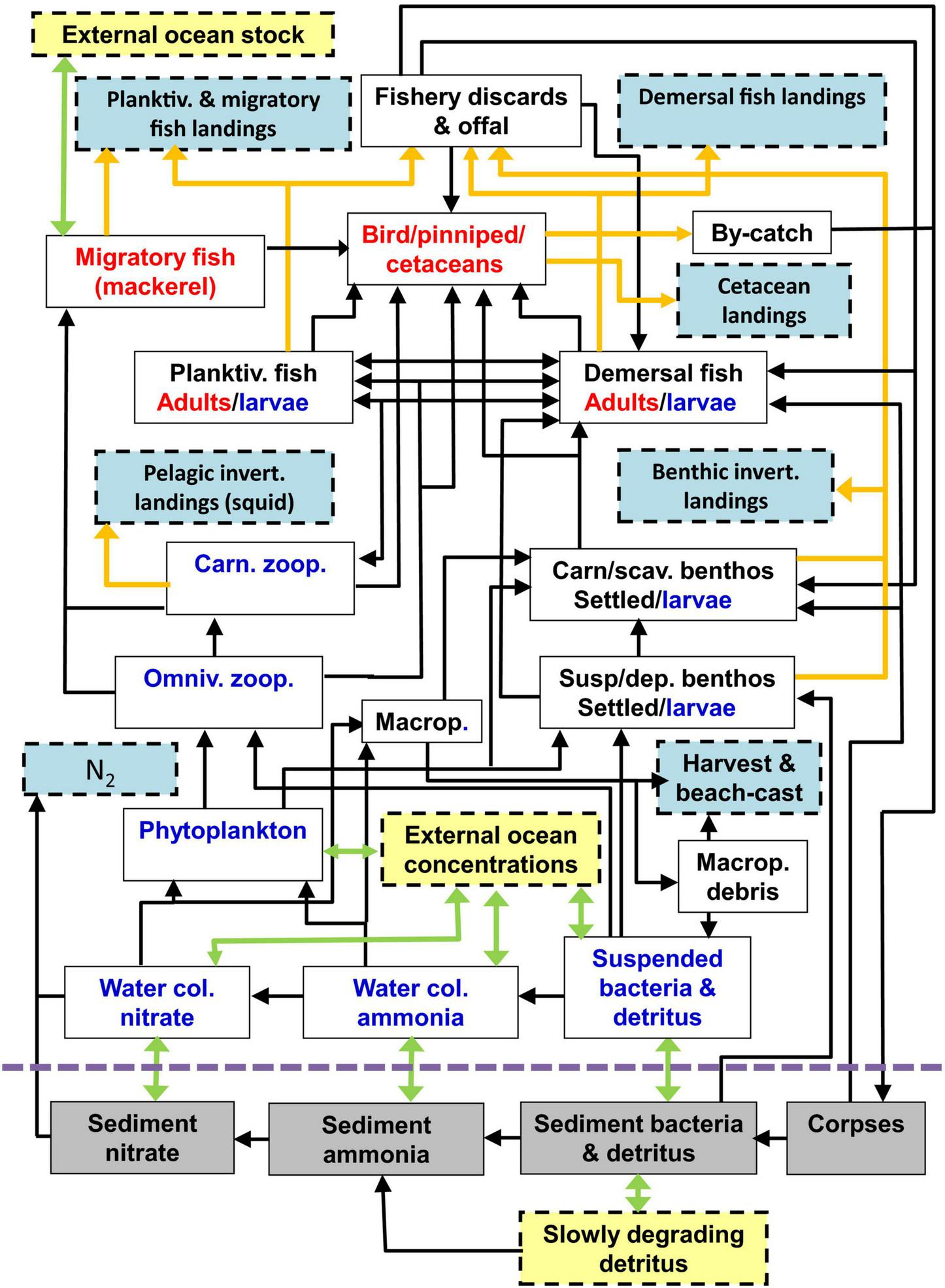
Schematic of the food web compartments of the StrathE2E2 model. Green arrows represent advection, mixing, and migration, orange arrows represent fishery-related fluxes, black arrows represent biological fluxes. Red labelled components are active migrators while blue are subject to passive advection and mixing, and black are anchored. Pale blue boxes represent quantities that are exported from the model while yellow are imported. The model also includes fluxes from living components to ammonia, detritus, and corpses due to excretion, defecation, and death, but these are not shown for clarity. Also for clarity, birds, pinnipeds, and cetaceans are combined as a single box in the figure, but in the model are treated separately. The abbreviation “Macrop” is shorthand for macrophytes. Diagram reproduced from Heath et al. (2020).
The model represents the time-dependent dynamics of the ecosystem components in a spatial region which is assumed to be consist of an offshore/deep zone and an inshore shallow zone which are each horizontally homogeneous. The offshore zone has an upper layer and a deep layer, whereas the inshore zone is a single homogenous compartment. The upper layer exchanges with the inshore zone and with the deep water. The inshore area is strongly influenced by freshwater inputs and tidally-driven exchange with the upper offshore layer, whereas the offshore upper and lower layers are most impacted by exchange with the open ocean (see Figure 2 in Heath et al., 2020). The inshore and offshore seabeds are each divided into discrete habitat types comprising exposed rock and up to three compartments of different sediment properties per zone. The sediment habitats are notionally mud, sand, and gravel, but are each defined by a single variable (median grain size) that is then used to derive a suite of geochemically relevant fixed (e.g., sediment permeability and porosity) and time-varying properties (e.g., natural disturbance rates). The geographic setting is defined by fixed properties (layer thicknesses and sediment porosity) and the time dependent drivers and boundary conditions. Biological properties are defined by parameters of the various uptake, excretion, mortality, and biogeochemical processes. Several key processes are temperature-dependent, including feeding and nutrient uptake, organism metabolism and nutrient regeneration (Heath et al., 2020). Typically, the model outputs data at daily time intervals and also delivers annual averaged concentrations and annually integrated rates. Biomasses can be recovered from the model units of gN or gC per m2 using information about the typical composition of functional groups (Beer, 1966; Heath et al., 2021).
We used the North Sea model as provided by the R-package and documented in Heath et al. (2021), choosing the 2003–2013 period as the reference baseline. The physical and chemical driving data used to force the model are described on page 15 and Table 9 of Heath et al. (2021).
The model was run for 100 years, and the last 20 years was taken to represent an equilibrium state. All components except birds and mammals typically attained equilibrium after 30 years or less, with birds and mammals taking about twice as long, so the equilibrium assumption was generally valid. The model has 12 idealised gear types (pelagic trawls, sandeel and sprat trawls, longline mackerel, beam trawl demersal, demersal seine, demersal otter trawl, demersal longline, beam trawl shrimp, Nephrops trawl, creels/pots, mollusc dredge, and whalers–Heath et al., 2021), representing the impacts of fleets targeting demersal, carnivorous benthos, and filter feeding benthos, and taking account of the seabed physico-chemical impacts of bottom trawling (Eigaard et al., 2015). We considered 16 fisheries scenarios, in which the harvesting of demersal and pelagic stocks was independently allowed to take one of four values, unfished (“U”), and 50% (“L”), 100% (“M”), and 200% (“H”) of recent (2000–2013) fishing (see Table 1). Other fleets with less severe direct effects on demersal and pelagic stocks were assumed to fish at 2000–2013 levels, apart from the unfished “UU” scenarios, where all fleets stayed in port. High (“H”) levels of fishing in this analysis approximate to the situation between 1970 and 2000 when fishing was inadequately regulated and stocks were undergoing depletion (Caswell et al., 2020; North Sea case study), low (“L”) levels would be consistent with well-regulated fishery managed in accordance with the principles of the Common Fisheries Policy or CFP (EU, 2013, 2015), whilst unfished states correspond with a pristine ecosystem. Three simple climate scenarios (temperatures unchanged at the 2000–2013 mean, uniform 2°C warming, and uniform 4°C warming, with no change in the amplitude of the seasonal cycle, ocean currents, storminess, or river run-off) were additionally considered for each of the 16 fisheries scenarios, making 48 combined fisheries and warming scenarios in total. The unchanged temperature scenarios are not realistic but provide an indicative baseline for evaluating the impacts due to fishing alone and in combination with warming. Traditionally, a warming of 2°C has been seen as the upper limit of change that can be accepted if “dangerous climate change” (i.e., outside the experience of the last 100,000 years—Nordhaus, 1977; Carbon Brief, 2014) is to be avoided, and there is a policy commitment brought into legal force by the Paris climate Agreement (UN, 2015) to stay below this threshold, but few concrete steps have been taken in this direction as of yet and a warming of 4°C by 2100 seems more likely (e.g., NASA, 2015).
Results
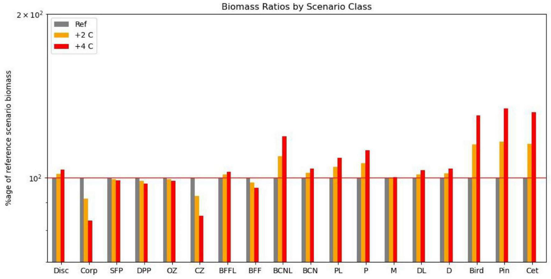
Equilibrium abundances of broad ecosystem components were compared for the various scenarios. These are expressed as percentages of the reference run (historic levels of fishing, “M,” and no climate warming) and are shown in Table 1. Underlying patterns of response to warming were illustrated by comparing the 16 fishing scenarios and no warming with the same fishing scenarios and warming of either 2 or 4°C, and are shown in Figure 2A. Responses to fishing are shown for five scenarios (unfished, low pelagic/high demersal, historic, high pelagic/low demersal, and high) compared with the reference case (no warming, 2000–2013 fishing) in Figure 2B.
FIGURE 2
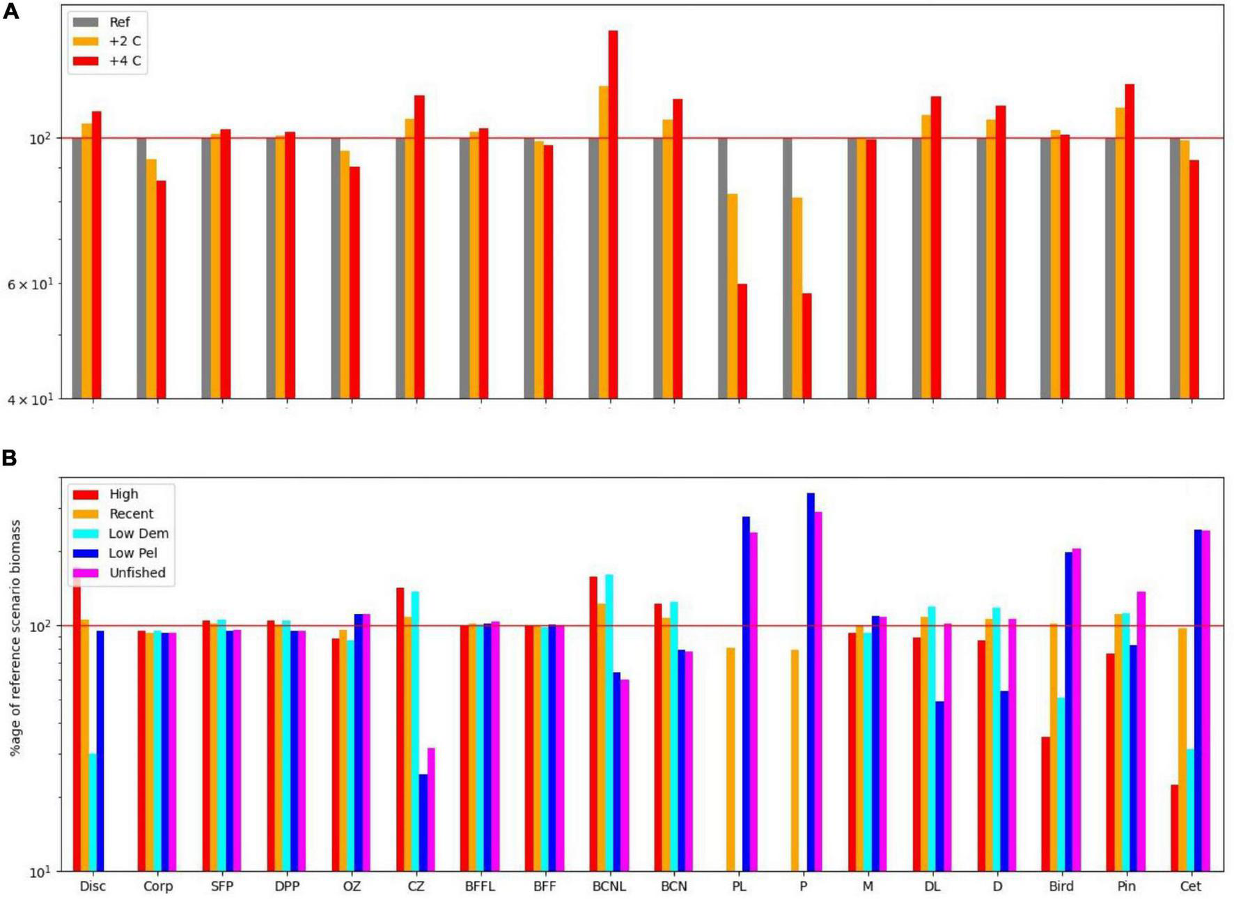
(A) Impact on functional groups across all fishing scenarios for the reference climate, and for warming of 2 and 4 centigrade. (B) Impact on functional groups across all climate, and benthic fishing scenarios for (i) high demersal and pelagic effort, (ii) medium demersal and pelagic effort, (iii) low pelagic effort, (iv) low demersal but high pelagic effort, and (v) low demersal and pelagic effort. Disc, discards; Corp, corpses; SFP, surface phytoplankton; DPP, deep phytoplankton; OZ, omnivorous zooplankton; CZ, carnivorous zooplankton; P, pelagic fish; PL, pelagic larvae; D, demersal fish; DL, demersal larvae; BFFL, benthic filter feeder larvae; BFF, benthic filter feeders; BCNL, benthic carnivore larvae; BCN, benthic carnivores; Bird, birds; Pin, pinnipeds; Cet, cetaceans.
Several broad patterns are clear and are shown schematically in Figure 3. Warming leads to an increase in primary productivity and the biomasses of ecosystem components with the exception of omnivorous zooplankton, benthic filter feeders, and pelagic fish. Effects are roughly double for 4°C warming compared with 2°C warming (Figure 2A), though the response profile is the same. Overfishing removes biomass from higher trophic levels in the ecosystem. Top predators and all fish groups decline, along with omnivorous zooplankton, whilst all other lower trophic groups become more abundant (Figure 3B). Stopping fishing results in higher biomass across all top predators and fish, with cascading effects at lower trophic levels. Carnivorous zooplankton and benthic carnivores lose out in terms of biomass as do phytoplankton, whilst the intermediate trophic level of omnivorous zooplankton and benthic filter feeders benefit. The impacts of stopping fishing are not the direct opposite of overfishing. If pelagic fishing is reduced whilst demersal fishing increases, there are mixed impacts across the foodweb. Seals lose out whilst other top predators benefit, reflecting an increase in pelagic fish and decrease in demersal fish, but impacts on lower trophic levels are similar to the unfished case (Figure 3D).
FIGURE 3
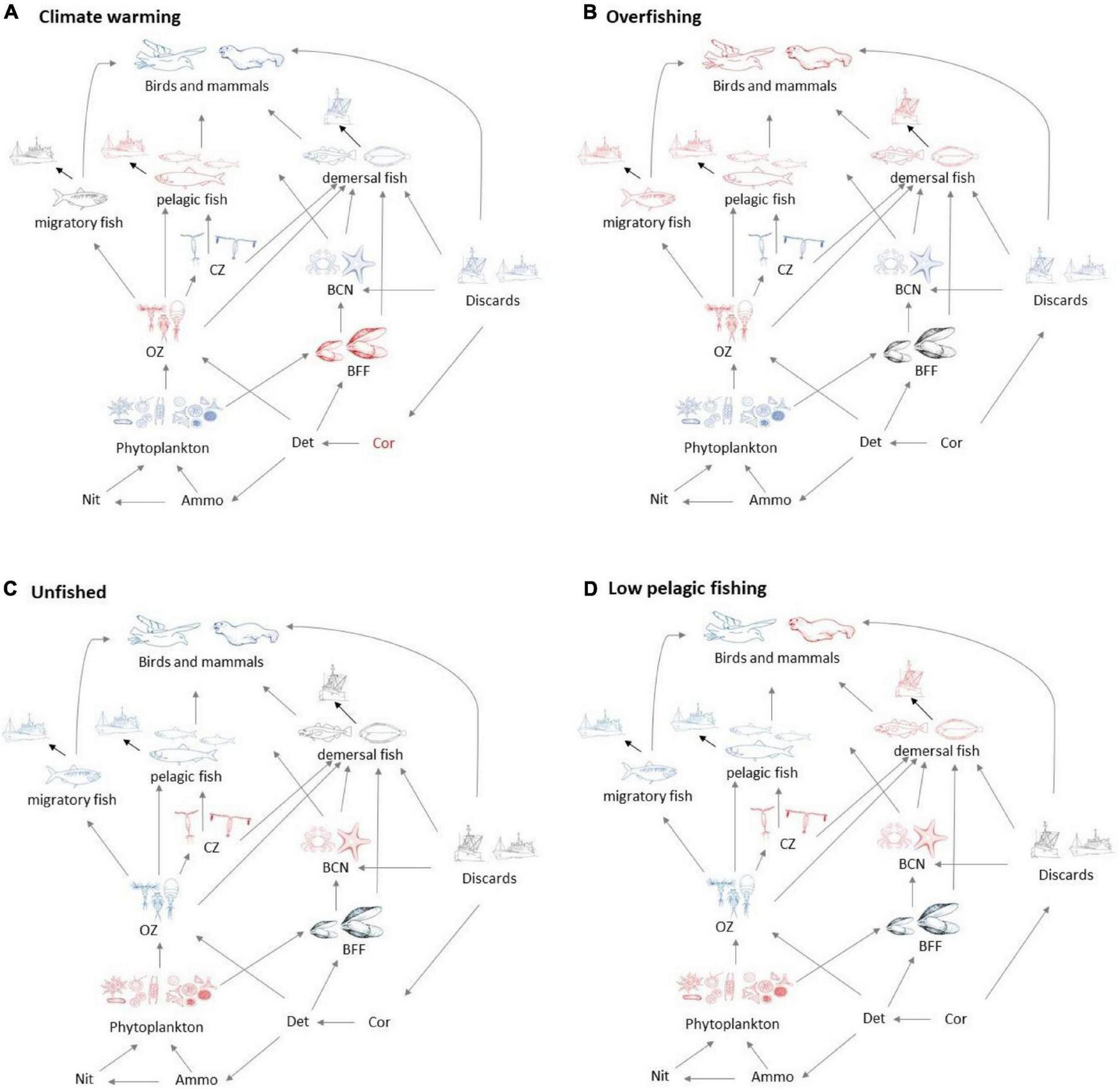
Schematic showing broad foodweb impacts of (A) warming and (B) overfishing compared with (C) the unfished state without warming and (D) states with low pelagic but high demersal fishing. All states are shown relative to recent history (no warming, medium levels of demersal, and pelagic fishing). Blue groups have increased biomass, and red groups reduced biomass, whilst grey indicates little change, except for discards in the unfished scenarios, which are zero.
Figure 4 shows how the form of the foodweb changes under warming conditions with reference level fishing on the left, and 5 fishing scenarios for 0, 2, and 4°C warming on the right. Whereas warming impacts on the size (total biomass) of the ecosystem, with modest shifts in functioning, fishing acts in the opposite manner with large shifts in function but little change in ecosystem-size, as shown by the larger spread of points on the right-hand side of Figure 4. High levels of fishing shift the system from pelagic toward benthic and, to a lesser extent, demersal group dominance, whilst birds, and cetaceans both fare poorly, with the reduced number of top predators becoming dominated by seals. Further down the food chain, carnivorous zooplankton and benthos gain at the expense of omnivorous zooplankton and benthic filter feeders due to predation release. Clustering of the fisheries scenarios into two groups suggests that the ecosystem can flip between demersal and pelagic states. The pelagic foodweb is highly geared so that small changes in predators and/or prey can have large impacts on pelagic biomass. Pelagic adults prey on their own larvae, demersal larvae, and omnivorous zooplankton, whilst demersal fish prey on pelagic adults and several other groups. This means that pelagic adults can stabilise at high abundance whilst keeping demersals in check through predation on their larvae, but alternatively, demersals can stabilise at high abundance whilst keeping pelagics in check through predation on their adults. Which state emerges can depend on fishing rates, but also critically on omnivorous zooplankton. If the latter are abundant, this supports pelagic stocks and keeps demersals in check. If they become depleted, pelagic fish eat their own larvae, and are not productive enough to keep demersals in check, further depleting the pelagic population. The metabolic demand of omnivorous zooplankton is sensitive to temperature, and increases significantly with warming, resulting in a shift toward demersals, other things being equal. We confirmed this was driving the changes by reducing this demand by 25%, leading to the changes shown in Figure 5, with pelagics now being favoured by warming.
FIGURE 4
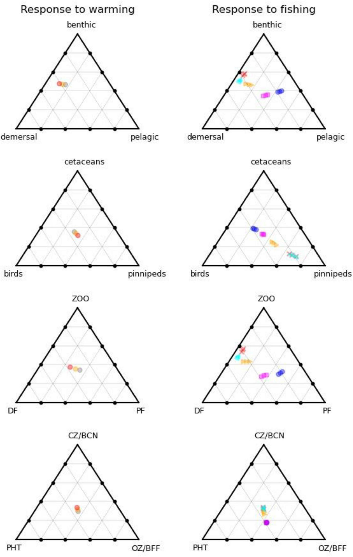
Foodweb pathways of different ecosystem compartments as a function of warming (left) and fishing (right). On the left-hand side, grey dots are the reference climate, orange 2C warming, and red 4C warming, all for recent historic levels of fishing. On the right-hand side, magenta squares are unfished, cyan triangles low demersal fishing, blue circles low pelagic fishing, orange triangles medium (recent historic fishing), and red crosses high fishing, all for the reference climate. Different positions on the triangles indicate differences in the relative partitioning of biomass between the three categories considered.
FIGURE 5
Impact on functional groups across all fishing scenarios for the reference climate, and for warming of 2 and 4 centigrade if omnivorous zooplankton metabolic demand is decreased by 25%. Disc, discards; Corp, corpses; SFP, surface phytoplankton; DPP, deep phytoplankton; OZ, omnivorous zooplankton; CZ, carnivorous zooplankton; P, pelagic fish; PL, pelagic larvae; D, demersal fish; DL, demersal larvae; BFFL, benthic filter feeder larvae; BFF, benthic filter feeders; BCNL, benthic carnivore larvae; BCN, benthic carnivores; Bird, birds; Pin, pinnipeds; Cet, cetaceans.
We also compared the relative impacts of warming and fishing on the 18 functional groups for this collection of scenarios (Table 2). As suggested in Figure 4, differences between overfishing and no fishing were overall greater than for warming of 4°C, but warming was more important for demersal fish, benthic filter feeders and corpses, whilst both had similar impacts on seals, omnivorous zooplankton, and carnivores. In this model, warming seems to support higher levels of fishing on demersal stocks, but lower on pelagic stocks. Pelagic fish are disproportionally dependent upon omnivorous zooplankton for food, and liable to suffer from cannibalism of their own larvae and enhanced predation from adult demersals if their zooplankton prey becomes depleted. We confirmed this sensitivity by reducing the parameter controlling metabolic uptake of omnivorous zooplankton by 25%; this resulted in increased abundance of omnivorous zooplankton and pelagic fish with warming of 2 and 4°C.
TABLE 2
| Climate warming more Important | Similar | Fishing more important |
| Demersal larvae Demersal fish Benthic filter feeders Corpses |
Surface phytoplankton Omnivorous zooplankton Benthic carnivores Pinnipeds |
Deep phytoplankton Carnivorous zooplankton Pelagic fish and larvae Migratory fish Discards Birds Cetaceans |
The relative importance of fishing and climate across scenarios for the StrathE2E2 functional groups.
Discussion
Our study found a trophic cascade in the ecosystem as a response to warming, which is driven by the increase in primary productivity, leading to an increase in the biomass of demersal fish relative to pelagic fish. In contrast, the response to fishing disproportionately affects the higher trophic levels of the ecosystem, both directly in terms of fish removed, and indirectly via impacts on top predators through food competition. Consequently, we found that fishing could have greater impacts on the pattern of energy flows and ecosystem function than warming, even though the latter had larger impacts on overall ecosystem productivity, at least for the scenarios considered here. This means that if we monitor ecosystem components at the broad scale, we can ensure that fisheries are being managed in a way that does not negatively impact ecosystem function and hinder the achievement of Good Environmental Status.
The main exception to productivity-driven warming responses was in the response of pelagic fish, and their key prey omnivorous zooplankton, whose biomasses decrease despite the ecosystem being more productive. This is down to the interplay of the following factors: (a) pelagic fish and larvae have fewer alternative prey choices in the foodweb than demersals, (b) pelagics are particularly dependent upon omnivorous zooplankton and their own larvae, (c) pelagics eat demersal larvae, whilst demersals eat pelagic adults, (d) omnivorous zooplankton have high metabolic requirements and readily become nitrogen limited in a warmer world, causing their abundance to decrease. The result is a trophic cascade, in which pelagics have less zooplankton to eat, consume a greater proportion of their own larvae and are less able to exert control on demersal stocks, which increase in abundance and predate on pelagic adults, keeping their numbers low. We confirmed this by reducing the metabolic demand of the omnivorous zooplankton by 25%, which was enough to halt the trophic cascade, and allow pelagic abundance to increase with warming and net productivity alongside other functional groups. If the simulated response is realistic, pelagic stocks may be at high risk of depletion in the future as warming continues, especially if fishing on demersal stocks continues to decline. However, it should be noted that model outputs are sensitive to a number of parameters involving omnivorous zooplankton (Heath et al., 2021). In particular, the physiological parameters controlling this behaviour were fixed from literature sources (Heath et al., 2021), and may change with shifting community composition under future climatic and environmental pressures. Further work is needed to confirm that this functional grouping is key to the foodweb, and to improve its representation in models.
Our responses to warming were driven by increases in primary production. This is in agreement with the end-to-end study of Griffith et al. (2012) who found that whilst ocean acidification had negative effects on productivity, they were over-ridden by the impacts of warming, leading to projected future increases in biomass. It is also broadly consistent with findings from ERSEM in the North Sea (van der Molen et al., 2013—though in their study demersal fish abundance increases at the expense of benthic rather than pelagic as here) as well as some other past studies. For example, Chavez et al. (2011) found that primary productivity increased with warming in the 20th Century, and they predicted that it would continue to do so in the future, whilst Simpson et al. (2011) reported that three times more species were increasing in abundance than decreasing. Hernant et al. (2010) found in their study of Bay of Biscay flatfish that there were more winners than losers with warming, though they reported that biomass gains were mainly in smaller species of lesser commercial interest. Van Leeuwen et al. (2021) also predict that net primary productivity will increase in the future in their end-to-end study of fishing and climate change impacts in the Gulf of Ancud, Chile.
However, our findings are in contrast with the multimodel intercomparison of Lotze et al. (2019), which suggested that primary productivity would decline in the future for every scenario they examined. The impact of future warming on ecosystem productivity remains highly uncertain, not least given the deficiencies in many global models of biogeochemical cycles (Anugerahanti et al., 2021).
Our study supports the use of end-to-end modelling when ascertaining impacts of human activities and climate change on GES. If we assume that GES is defined relative to the unfished (potential recovery) state, then we can evaluate departures from it (magenta squares in Figure 4) either in terms of distance [changes in the size of the ecosystem or relative balance between, e.g., realms (Figure 4, top right), trophic structure (Figure 4, lower right) or top predators (Figure 4, second row right)], and the timescale of recovery to unfished levels of the slowest acting ecosystem component [following the suggestion of Rossberg et al. (2017)]. Scenarios that take too long to recover the unfished state if fishing ceases, or are too far from it in terms of absolute biomasses or key biomass ratios, would then be deemed inconsistent with GES.
Caveats
We find responses to warming and fishing that are consistent with foodweb dynamics assuming that productivity increases in a warmer world, and supported by sensitivity studies in the case of pelagic fish and omnivorous zooplankton. Assessing the true statistical significance of these responses might require large numbers of replicates to explore variability associated with scenario boundary conditions, which is beyond the scope of this work. However, in the absence of this, it can be noted that many of the responses are (a) large, (b) coherent across warming or fishing scenarios, and (c) makes sense in the context of the model foodweb, so it seems reasonable to postulate that the observed changes might be significant. Further work is needed to prove this definitively or refute it, however.
Several further caveats need to be borne in mind when considering the findings of this study. The model framework has only a simple functional group structure, so is only able to suggest that broad patterns of change might be likely. It is not the right model to use when asking more specific questions, such as “will cod biomass increase as a result of the projected changes in climate and fishing.” For whilst we find that “demersal” biomass is likely to increase in a warmer world, this does not imply that all demersals will gain; some such as cod that are toward the warm limit of their range already, may fare less well than others that are nearer their colder limits in the North Sea (Rijnsdorp et al., 2010). So, the findings refer more to groups of species such as “gadoids” rather than the individual species of cod, haddock, whiting, grey gurnard, etc.
Secondly, although 48 scenarios were considered, this is only a small fraction of the possible future scenarios for fishing and climate change. We considered only the impacts of warming, not acidification, eutrophication, or circulation change, although the model could be used to examine this further. The fishing scenarios were bounded by estimates of historic fishing and FMSY, and only the impacts of 12 major fleet groupings (Heath et al., 2021) were considered. Whilst we considered the unfished state for each level of warming, it may be necessary to consider more scenarios in which fishing mortality is reduced below FMSY to unmask any feedbacks associated with the recovery of the seabed to a less impacted state, even though the model does in principle allow this to be investigated.
Thirdly, the assumptions about discarding are based upon what has been observed between 2003 and 2013. With the coming into force of the Landings Obligation (EU, 2015), it is likely that discarding will reduce significantly, irrespective of the changes observed here. The wider impact of this regulation remains to be ascertained.
Fourthly, our results are conditional on the StrathE2E2 model structure and fitted parameter set. Whilst it has the advantage of representing the ecosystem from end-to-end including biogeochemistry, the main compromise is in the reduced number of ecosystem components, so it would be beneficial to compare outcomes with models that can resolve more biological components such as Atlantis (Audzijonyte et al., 2019a), perhaps using the methodology of Spence et al. (2018) to combine model outputs. This would help to inform the minimum number of functional groups needed to describe an entire ecosystem, whilst parameter uncertainty could be investigated using Monte Carlo methods (Hastings, 1970) in future work, particularly given the apparently key role of omnivorous zooplankton in the foodweb and the uncertainty of the fitted parameters associated with it.
It should be noted that StrathE2E2 does not resolve size structure within individual groups. Some studies (Foster and Hirst, 2012; Cheung et al., 2013; Queirós et al., 2018; Audzijonyte et al., 2019b), suggest that warming will reduce the maximum size of fish, thus there might be a greater biomass of smaller fish that are of lesser commercial interest, so the increase in NPP and ecosystem size seen with warming does not imply that North Sea fisheries will be more productive and valuable in the future.
Summary and Conclusion
In this study we have used the “big picture” model StrathE2E2 (Heath et al., 2020) to look at the North Sea ecosystem response to various scenarios of warming and fishing, exploring the manner in which top down (fishing) and bottom up (warming) effects alter the overall structure and function of the foodweb, and investigate the extent to which monitoring of broad ecosystem groups can tell us whether management is successfully achieving Good Environmental Status as mandated by legislation.
We found that warming and fishing have contrasting effects on the structure and function of the North Sea ecosystem. Warming primarily changes the size of the ecosystem through its effects on primary productivity. In this case productivity increases with warming and ecosystem biomass rises with it. This contrasts with the recent expectation of decline and ecosystem shrinkage (Lotze et al., 2019) but has some support in the literature (e.g., Chavez et al., 2011) and is consistent with ERSEM biogeochemical modelling (van der Molen et al., 2013). On the other hand, fishing tends to reduce biomass at the top of the foodweb, with cascading effects leading to some increases elsewhere. Thus, to first order, warming changes the size of the ecosystem with modest impacts on function, fishing changes ecosystem function with modest effects on its size. There are two obvious corollaries: (1) monitoring of broad ecosystem groups may be able to untangle the effects of fishing and warming, and (2) monitoring of ecosystem function is needed to ensure that Good Environmental Status is not compromised by fishing activity.
A small number of functional groups may be able to succinctly summarise the state of the ecosystem in terms of energy transfer between trophic levels, and between demersal, pelagic, and scavenging foodwebs. These energy transfers have implications for the efficiency of fish production, and ecosystem well-being and resilience; therefore it makes sense to monitor them to inform assessments of ecosystem status. We therefore propose a minimum set of 10 broad functional groups that should be monitored in order to facilitate this assessment: deep phytoplankton, surface phytoplankton, omnivorous zooplankton, carnivorous zooplankton, pelagic fish, demersal fish, benthic filter feeders, benthic suspension feeders, birds and mammals, and discards. As part of this recommendation, we emphasise that both broad categories of benthos, suspension feeders, and carnivorous scavengers should have their biomasses monitored.
The main exception to the broad picture concerned the response of pelagic fish, omnivorous zooplankton, and benthic filter feeders, which lost biomass under warming, even though the ecosystem became more productive. This was tied up with a trophic cascade in which the increased metabolic demands of omnivorous zooplankton in a warmer world decreased the prey available to pelagic fish and caused the ecosystem to shift in favour of demersals. This cascade is dependent upon both the structure of the foodweb and values of fitted parameters in StrathE2E2, but is consistent with the meta-analysis of Hulot et al. (2014), and if it is realistic, pelagic fisheries are likely to be at increased risk in the future, a risk that could be compounded by the ongoing reduction in demersal fishing effort. This is a risk that should be closely monitored whilst the likelihood of such a trophic cascade is evaluated using alternate model structures and measurements of key processes. Meanwhile our findings suggest the need to improve our basic understanding of bottom-up processes, improve our representation of them in models (e.g., more zooplankton groups rather than generic “background resource”) and ensure that our ecosystem models can capture limitation by nitrogen and other elements, and not just food/energy uptake.
Publisher’s Note
All claims expressed in this article are solely those of the authors and do not necessarily represent those of their affiliated organizations, or those of the publisher, the editors and the reviewers. Any product that may be evaluated in this article, or claim that may be made by its manufacturer, is not guaranteed or endorsed by the publisher.
Statements
Data availability statement
The original contributions presented in the study are included in the article/supplementary material, further inquiries can be directed to the corresponding author/s.
Author contributions
RT adapted the model and designed the experiments. MH developed the model based on the need for a “big picture” end to end model. NA, GS, NN, IP, and CL all helped with framing the study in the context of indicators of ecosystem impact and GES. MP and MH provided valuable insights into the operation of the model. CL secured the funding along with RT. All authors contributed to the final manuscript.
Funding
This study was funded by the EU project “Addressing gaps in biodiversity indicator development for the OSPAR Region from data to ecosystem assessment: Applying an ecosystem approach to (sub) regional habitat assessments (EcApRHA, grant 11.0661/2015/712630/SUB/ENVC.2 OSPAR)” and by the UKI Government Department for Environment, Food and Rural Affairs (DEFRA), grant MA016A. Additional funding for RT has been provided by the EU Horizon 2020 project PANDORA (grant agreement No 773713) and for CL by the EU Horizon 2020 project FutureMARES (grant agreement No 869300).
Acknowledgments
We are grateful to editor Tomaso Fortibuoni and three referees whose helpful comments have improved the framing of the study and the quality of the discussion.
Conflict of interest
The authors declare that the research was conducted in the absence of any commercial or financial relationships that could be construed as a potential conflict of interest.
References
1
Anugerahanti P. Kerimoglu O. Smith S. L. (2021). Enhancing ocean biogeochemical models with phytoplankton variable composition.Front. Mar. Sci.8:675428. 10.3389/fmars.2021.675428
2
Audzijonyte A. Barreche D. R. Baudron A. R. Belmaker J. Clark T. D. Marchall C. T. et al (2019a). Is oxygen limitation in warming waters a valid mechanism to explain decreased body sizes in aquatic ectotherms?Glob. Ecol. Biogeogr.2864–77. 10.1111/geb.12847
3
Audzijonyte A. Pethybridge H. Porobic J. Gorton R. Kaplan I. Fulton E. A. (2019b). Atlantis: a spatially explicit end-to-end marine ecosystem model with dynamically integrated physics, ecology and socio-economic modules.Methods Ecol. Evol.101814–1819. 10.1111/2041-210X.13272
4
Beer J. R. (1966). Studies on the chemical composition of the major zooplankton groups in the Sargasso Sea off Bermuda.Limnol. Oceanogr.11520–528. 10.4319/lo.1966.11.4.0520
5
Bolam S. G. Fernandes T. F. Huxham M. (2002). Diversity, biomass, and ecosystem processes in marine benthos.Ecol. Monogr.72599–615. 10.1890/0012-9615(2002)072[0599:DBAEPI]2.0.CO;2
6
Borja A. Elliott M. Andersen J. H. Cardoso A. C. Carstensen J. Ferreira J. G. et al (2013). Good environmental status of marine ecosystems: what is it and how do we know when we have attained it?Mar. Pollut. Bull.7616–27. 10.1016/j.marpolbul.2013.08.042
7
Borja A. Prins T. C. Simboura N. Andersen J. H. Berg T. Marques J.-C. et al (2014). Tales from a thousand and one ways to integrate marine ecosystem components when assessing the environmental status.Front. Mar. Sci.1:72. 10.3389/fmars.2014.00072
8
Bradley D. Merrifield M. Miller K. M. Lomonico S. Wilson J. R. Gleeson M. G. (2019). Opportunities to improve fisheries management through innovative technology and advanced data systems.Fish Fish.20563–584. 10.1111/faf.12361
9
Butenshon M. Clark J. Aldridge J. N. Allen J. I. Artioli Y. Blackford J. et al (2016). ERSEM 15.06: a generic model for marine biogeochemistry and the ecosystem dynamics of the lower trophic levels.Geosci. Model Dev.91293–1339. 10.5194/gmd-9-1293-2016
10
Carbon Brief (2014). Carbon Brief.Available online at: https://www.carbonbrief.org/two-degrees-the-history-of-climate-changes-speed-limit(accessed February 28, 2021).
11
Caswell B. A. Klein E. S. Alleway H. K. Ball J. E. Botero J. Cardinale M. et al (2020). Something old, something new: historical perspectives provide lessons for blue growth agendas.Fish Fish.21774–796. 10.1111/faf.12460
12
Chassot E. Mélin F. Le Pape O. Gascuel D. (2007). Bottom-up control regulates fisheries production at the scale of eco-regions in European seas.Mar. Ecol. Prog. Ser.34345–55. 10.3354/meps06919
13
Chavez F. P. Messie M. Pennington J. T. (2011). Marine primary production in relation to climate variability and change.Annu. Rev. Mar. Sci.3227–260. 10.1146/annurev.marine.010908.163917
14
Cheung W. W. L. Sarmiento J. L. Dunne J. Frolicher T. L. Lam V. W. Y. Deng Palomers M. L. et al (2013). Shrinking of fishes exacerbates impacts of global ocean changes on marine ecosystems.Nat. Clim. Change3254–258. 10.1038/nclimate1691
15
Christensen V. Walters C. J. (2004). Ecopath with Ecosim: methods, capabilities and limitations.Ecol. Modell.172109–139. 10.1016/j.ecolmodel.2003.09.003
16
Eigaard O. R. Bastardie F. Breen M. Dinesen G. E. Hintzen N. T. Laffargue P. et al (2015). Estimating seabed pressure from demersal trawls, seines, and dredges based on gear design and dimensions.ICES J. Mar. Sci.73i27–i43. 10.1093/icesjms/fsv099
17
EU (2008). Directive 2008/56/EC of the European Parliament and of the Council of 17 June 2008 Establishing a Framework for Community Action in the Field of Marine Environmental Policy (Marine Strategy Framework Directive).Brussels: European Communities.
18
EU (2013). Regulation (EU) 1380/2013 of the European Parliament and of the Council of 11 December 2013 on the Common Fisheries Policy, Amending Council Regulations (EC) No 1954/2003 and (EC) No 1224/2009 and Repealing Council Regulations (EC) No 2371/2002 and (EC) No 639/2004 and Council Decision 2004/585/EC.Brussels: European Communities.
19
EU (2014). Establishing a Framework for Maritime Spatial Planning. 2014/89/EU.Brussels: Official Journal of the European Union.
20
EU (2015). Regulation (EU) 2015/812 of the European Parliament and of the Council of 20 May 2015 Amending Council Regulations (EC) No 850/98, (EC) No 2187/2005, (EC) No 1967/2006, (EC) No 1098/2007, (EC) No 254/2002, (EC) No 2347/2002 and (EC) No 1224/2009, and Regulations (EU) No 1379/2013 and (EU) No 1380/2013 of the European Parliament and of the Council, as Regards the Landing Obligation, and Repealing Council Regulation (EC) No 1434/98.Brussels: European Communities.
21
FAO (1995). Reference Points for Fisheries Management. FAO Fisheries Technical Paper No 347. Rome: FAO.
22
Foster J. Hirst A. G. (2012). The temperature-size rule emerges from ontogenetic differences between growth and development rates.Funct. Ecol.26483–492. 10.1111/j.1365-2435.2011.01958.x
23
Fulton E. A. (2010). Approaches to end-to-end ecosystem models.J. Mar. Syst.81171–183. 10.1016/j.jmarsys.2009.12.012
24
Gamfeldt L. Lefcheck J. S. Byrnes J. E. Cardinale B. J. Duffy J. E. Griffin J. N. (2014). Marine biodiversity and ecosystem functioning: what’s known and what’s next?PeerJ2:e249v1. 10.7287/peerj.preprints.249v1
25
Giricheva E. (2015). Aggregation in ecosystem models and model stability.Prog. Oceanogr.134190–196. 10.1016/j.pocean.2015.01.016
26
Griffith G. P. Fulton E. A. Gorton R. Richardson A. J. (2012). Predicting interactions among fishing, ocean warming, and ocean acidification in a marine system with whole-ecosystem models.Conserv. Biol.261145–1152. 10.1111/j.1523-1739.2012.01937.x
27
Hastings W. K. (1970). Monte Carlo sampling methods using Markov chains and their applications.Biometrika5797–109. 10.1093/biomet/57.1.97
28
Heath M. R. (2012). Ecosystem limits to food web fluxes and fisheries yields in the North Sea simulated with an end-to-end food web model.Prog. Oceanogr.10242–66. 10.1016/j.pocean.2012.03.004
29
Heath M. R. Speirs D. C. McDonald A. Wilson R. (2021). StrathE2E2 Version 3.3.0: Implementation for the North Sea.Available online at: https://marineresourcemodelling.gitlab.io/(accessed January 31, 2022).
30
Heath M. R. Speirs D. C. Steele J. H. (2014). Understanding patterns and processes in models of trophic cascades.Ecol. Lett.17101–114. 10.1111/ele.12200
31
Heath M. R. Speirs D. C. Thurlbeck I. Wilson R. (2020). StrathE2E2: an R package for modelling the dynamics of marine food webs and fisheries.Methods Ecol. Evol.12280–287. 10.1111/2041-210X.13510
32
Hernant M. Lobry J. Bonhommeau S. Pailard J.-C. Le Pape O. (2010). Impact of warming on abundance and occurrence of flatfish populations in the Bay of Biscay (France).J. Sea Res.6445–53. 10.1016/j.seares.2009.07.001
33
Hulot F. D. Lacroix G. Loreau M. (2014). Differential responses of size-based functional groups to bottom-up and top-down perturbations in pelagic food webs: a meta-analysis.Oikos1231291–1300. 10.1111/oik.01116
34
Hyder K. Rossberg A. G. Allen J. I. Austen M. C. Barciela R. M. Bannister H. J. et al (2015). Making modelling count - increasing the contribution of shelf-seas community and ecosystem models to policy development and management.Mar. Policy61291–302. 10.1016/j.marpol.2015.07.015
35
ICES (2015). Report of the Workshop on Guidance for the Review of MSFD Decision Descriptor 4 –Foodwebs II (WKGMSFDD4-II). ICES Document CM 2015\ACOM:49.Copenhagen: ICES.
36
Iwasa Y. Andreasen V. Levin S. (1987). Aggregation in model ecosystems. I. Perfect aggregation.Ecol. Modell.37287–302. 10.1016/0304-3800(87)90030-5
37
Kavanagh L. Galbraith E. (2018). Links between fish abundance and ocean biogeochemistry as recorded in marine sediments.PLoS One13:e0199420. 10.1371/journal.pone.0199420
38
Lotze H. K. Tittensor D. P. Bryndum-Bucholz A. Eddy T. D. Cheung W. W. L. Galbraith E. D. et al (2019). Global ensemble models reveal trophic amplification of ocean biomass declines with climate change.Proc. Natl. Acad. Sci.11612907–12912. 10.1073/pnas.1900194116
39
Mackinson S. Daskalov G. (2007). An ecosystem model of the North Sea to support an ecosystem approach to fisheries management: description and parameterisation.Sci. Ser. Tech. Rep.142:196.
40
Moreau J. De Silva S. S. (1991). Predictive Fish Yield Models for Lakes and Reservoirs of the Philippines, Vol. 319. Rome: Food and Agriculture Organization.
41
Morris D. Speirs D. Cameron A. Heath M. (2014). Global sensitivity of and end-to-end marine ecosystem model of the North Sea: factors affecting the biomass of fish and benthos.Ecol. Modell.273251–263. 10.1016/j.ecolmodel.2013.11.019
42
NASA (2015). Detailed Global Climate Change Predictions to 2100.Available online at: https://www.nasa.gov/press-release/nasa-releases-detailed-global-climate-change-projections(accessed December 21, 2021).
43
Nordhaus W. D. (1977). Economic growth and climate: the carbon dioxide problem.Am. Econ. Rev.67341–346.
44
Piroddi C. Akoglu E. Andonegi E. Bentley J. W. Celic I. Coll M. et al (2021). Effects of nutrient management scenarios on marine food webs: a pan-European assessment in support of the marine strategy framework directive.Front. Mar. Sci.8:596797. 10.3389/fmars.2021.596797
45
Queirós A. M. Fernandes J. Genevier L. Lynam C. P. (2018). Climate change alters fish community size-structure, requiring adaptive policy targets.Fish Fish.19613–621. 10.1111/faf.12278
46
Rice J. Arvanitidis C. Borja A. Frid C. Hiddink J. G. Krause J. et al (2012). Indicators for sea-floor integrity under the European marine strategy framework directive.Ecol. Indic.12174–184. 10.1016/j.ecolind.2011.03.021
47
Rijnsdorp A. D. Peck M. A. Engelhard G. H. Mollmann C. Pinnegar J. K. (2010). Resolving the effects of climate change on fish populations.ICES J. Mar. Sci.661570–1583. 10.1093/icesjms/fsp056
48
Rindorf A. Cardinale M. Shephard S. De Oliveira J. A. A. Hjorleifsson E. Kempf A. et al (2016). Fishing for MSY: can ‘pretty good yield’ ranges be used without impairing recruitment?ICES J. Mar. Sci.74525–534. 10.1093/icesjms/fsw111
49
Rossberg A. G. Uusitalo L. Berg T. Zaiko A. Chenuil A. Uyarra M. C. et al (2017). Quantitative criteria for choosing targets and indicators for sustainable use of ecosystems.Ecol. Indic.72215–224. 10.1016/j.ecolind.2016.08.005
50
Scott F. Blanchard J. L. Andersen K. H. (2014). mizer: an R package for multispecies trait-based and community size spectrum ecological modelling.Methods Ecol. Evol.51121–1125. 10.1111/2041-210X.12256
51
Simpson S. P. Jennings S. Johnston M. P. Blanchard J. L. Schon P. J. Sims D. W. et al (2011). Continental shelf-wide response of a fish assemblage to rapid warming of the sea.Curr. Biol.211565–1570. 10.1016/j.cub.2011.08.016
52
Speirs D. C. Guirey E. J. Gurney W. S. C. Heath M. R. (2010). A length-structured partial ecosystem model for cod in the North Sea.Fish. Res.106474–494. 10.1016/j.fishres.2010.09.023
53
Spence M. A. Blanchard J. L. Rossberg A. G. Heath M. R. Heymans J. J. Mackinson S. et al (2018). A general framework for comparing ecosystem models.Fish Fish.191031–1042. 10.1111/faf.12310
54
Teixeira H. Berg T. Fürhaupter K. Uusitalo L. Papadopoulou N. Bizsel K. C. et al (2014). Existing Biodiversity, Non-Indigenous Species, Food-Web and Seafloor Integrity GEnS Indicators (DEVOTES Deliverable 3.1) DEVOTES FP7 Project. 198.Available online at: http://www.devotes-project.eu(accessed December 21, 2021).
55
Thorpe R. B. De Oliveira J. A. A. (2019). Comparing conceptual frameworks for a fish community MSY (FCMSY) using management strategy evaluation—an example from the North Sea.ICES J. Mar. Sci.76813–823. 10.1093/icesjms/fsz015
56
Thurow F. (1997). Estimation of the total fish biomass in the Baltic Sea during the 20th century.ICES J. Mar. Sci.444–461. 10.1006/jmsc.1996.0195
57
UN (2015). Paris climate agreement.Int. Legal Mater.55740–755. 10.1017/S0020782900004253
58
van der Molen J. Aldridge J. N. Coughlan C. Parker E. R. Stephens D. Ruardij P. (2013). Modelling marine ecosystem response to climate change and trawling in the North Sea.Biogeochemistry113213–236. 10.1007/s10533-012-9763-7
59
van Deurs M. Brooks M. E. Lindegren M. Henricksen O. Rindorf A. (2020). Biomass limit reference points are sensitive to estimation method, time-series length, and stock development.Fish Fish.2218–30. 10.1111/faf.12503
60
Van Leeuwen S. M. Salgado H. Bailey J. L. Beecham J. Iriarte J. L. García-García L. et al (2021). Climate change, marine resources and a small Chilean community: making the connections.Mar. Ecol. Prog. Ser.680223–246. 10.3354/meps13934
61
Ware D. M. Thomson R. E. (2005). Bottom-up ecosystem trophic dynamics determine fish production in the Northeast Pacific.Science3081280–1284. 10.1126/science.1109049
Summary
Keywords
fisheries, North Sea, climate change, ecosystem modelling, MSFD, foodweb indicators, benthos, good environmental status
Citation
Thorpe RB, Arroyo NL, Safi G, Niquil N, Preciado I, Heath M, Pace MC and Lynam CP (2022) The Response of North Sea Ecosystem Functional Groups to Warming and Changes in Fishing. Front. Mar. Sci. 9:841909. doi: 10.3389/fmars.2022.841909
Received
22 December 2021
Accepted
18 February 2022
Published
04 April 2022
Volume
9 - 2022
Edited by
Tomaso Fortibuoni, Istituto Superiore per la Protezione e la Ricerca Ambientale (ISPRA), Italy
Reviewed by
Claudio Vasapollo, Istituto Superiore per la Protezione e la Ricerca Ambientale (ISPRA), Italy; Natalia Serpetti, Joint Research Centre, Italy; Cecilia Pinto, University of Genoa, Italy
Updates
Copyright
© 2022 Thorpe, Arroyo, Safi, Niquil, Preciado, Heath, Pace and Lynam.
This is an open-access article distributed under the terms of the Creative Commons Attribution License (CC BY). The use, distribution or reproduction in other forums is permitted, provided the original author(s) and the copyright owner(s) are credited and that the original publication in this journal is cited, in accordance with accepted academic practice. No use, distribution or reproduction is permitted which does not comply with these terms.
*Correspondence: Robert B. Thorpe, robert.thorpe@cefas.co.uk
This article was submitted to Marine Fisheries, Aquaculture and Living Resources, a section of the journal Frontiers in Marine Science
Disclaimer
All claims expressed in this article are solely those of the authors and do not necessarily represent those of their affiliated organizations, or those of the publisher, the editors and the reviewers. Any product that may be evaluated in this article or claim that may be made by its manufacturer is not guaranteed or endorsed by the publisher.