 Xiaochen Zhao1*†
 Victor H. Rivera-Monroy1*†
 Chunyan Li1,2†
 Ivan A. Vargas-Lopez1†
 Robert V. Rohli1,2†
 Z. George Xue1,2,3†
 Edward Castañeda-Moya4†
 Carlos Coronado-Molina5†
- 1Department of Oceanography and Coastal Sciences, College of the Coast and Environment, Louisiana State University, Baton Rouge, LA, United States
- 2Coastal Studies Institute, Louisiana State University, Baton Rouge, LA, United States
- 3Center for Computation and Technology, Louisiana State University, Baton Rouge, LA, United States
- 4Institute of Environment, Florida International University, Miami, FL, United States
- 5Everglades Systems Assessment Section, South Florida Water Management District, West Palm Beach, FL, United States
Environmental temperature is a widely used variable to describe weather and climate conditions. The use of temperature anomalies to identify variations in climate and weather systems makes temperature a key variable to evaluate not only climate variability but also shifts in ecosystem structural and functional properties. In contrast to terrestrial ecosystems, the assessment of regional temperature anomalies in coastal wetlands is more complex since the local temperature is modulated by hydrology and weather. Thus, it is unknown how the regional free-air temperature (TFree) is coupled to local temperature anomalies, which can vary across interfaces among vegetation canopy, water, and soil that modify the wetland microclimate regime. Here, we investigated the temperature differences (offsets) at those three interfaces in mangrove-saltmarsh ecotones in coastal Louisiana and South Florida in the northern Gulf of Mexico (2017–2019). We found that the canopy offset (range: 0.2–1.6°C) between TFree and below-canopy temperature (TCanopy) was caused by the canopy buffering effect. The similar offset values in both Louisiana and Florida underscore the role of vegetation in regulating near-ground energy fluxes. Overall, the inundation depth did not influence soil temperature (TSoil). The interaction between frequency and duration of inundation, however, significantly modulated TSoil given the presence of water on the wetland soil surface, thus attenuating any short- or long-term changes in the TCanopy and TFree. Extreme weather events—including cold fronts and tropical cyclones—induced high defoliation and weakened canopy buffering, resulting in long-term changes in canopy or soil offsets. These results highlight the need to measure simultaneously the interaction between ecological and climatic processes to reduce uncertainty when modeling macro- and microclimate in coastal areas under a changing climate, especially given the current local temperature anomalies data scarcity. This work advances the coupling of Earth system models to climate models to forecast regional and global climate change and variability along coastal areas.
1 Introduction
Among the key factors regulating climate and weather in a location, the temperature is the most recognized and widely measured. Because temperature is correlated to heat content, it has become a key proxy to evaluate climate change and its impact at the global scale. Indeed, the utility of temperature anomalies—the difference from an average or baseline of temperature over ~30 years—to identify variations in both climate and weather systems (Jones et al., 2012) makes temperature a critical variable to characterize not only climate variability and extreme changes in precipitation and humidity, but also major shifts in structural and functional properties of ecosystems (e.g., species diversity, net primary productivity (NPP), carbon storage). Yet a major knowledge gap is apparent due to data scarcity when comparing our level of understanding about the fluctuation and trajectory of temperature anomalies at the atmospheric level (e.g., heat storage, wind circulation) vs. their impact on ecological processes at the vegetation-soil interface in terrestrial and coastal ecosystems (e.g., soil respiration, organic matter decomposition, CO2 emissions; Figure 1). For instance, how the global temperature anomaly—for 2011–2020, presently estimated at +0.82°C above the 20th century average (NOAA State of the Climate: Global Climate Report, 2020)—propagates to ecosystems as successively finer scales across latitudinal gradients is poorly understood.
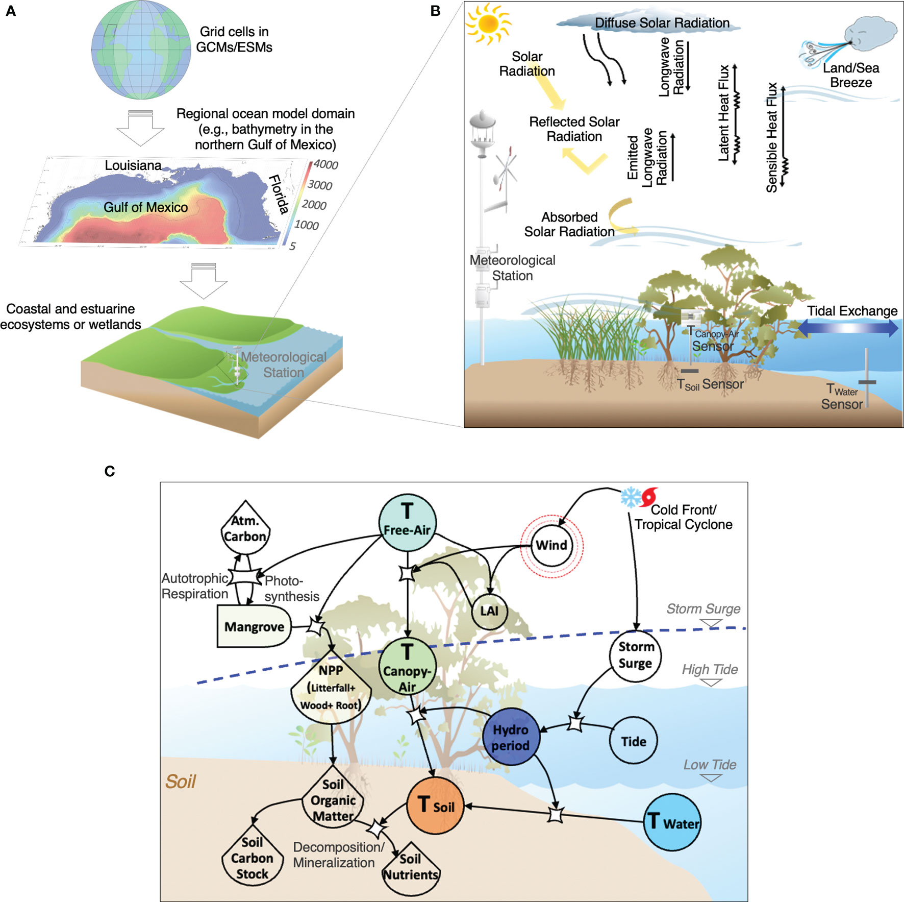
Figure 1 Conceptual diagram showing (A) grid cell in General circulation models (GCMs) or Earth system models (ESMs) downscaled to the regional ocean model domain (e.g., bathymetry in the northern Gulf of Mexico) and coastal/estuarine ecosystems or wetlands; (B) energy fluxes near ground in coastal wetlands, and (C) biogeochemical cycling in coastal wetlands regulated by local hydroperiod and microclimate temperature (i.e., soil and canopy air) under impacts of regional free-air temperature and extreme weather events, including tropical cyclones and cold fronts. The panel (B) is modified from Bonan (2008). Symbols in panel (C) are from Odum’s Energy Systems Language and the Integration and Application Network (https://www.osti.gov/biblio/5545893; https://ian.umces.edu/symbols). Abbreviations in panel (B, C): T, Temperature; Atm., Atmosphere; NPP, Net primary productivity; LAI, Leaf area index.
In the last decade, the lack of temperature data to identify long-term temperature anomalies at smaller scales (< 1 km) has become apparent as Earth system models (ESMs) are coupled to General circulation models (GCMs) to include ecosystem feedback processes. This gap in temperature data has complicated the representation of its direct effect on biogeochemical processes (e.g., greenhouses emissions) and ecosystem carbon sequestration and storage rates (Jones et al., 2019). Moreover, the GCM-ESMs coupling underscores the need to understand how temperature is modulated, for example, by the variable types of vegetation and extension (e.g., grass, shrubs, and forests), particularly in transitional zones or ecotonal regions (D'Odorico et al., 2013). Because vegetation phenology, crown architecture, and total area vary significantly across complex landscape mosaics that include a wide range of natural habitats and land units modified by human activities (e.g., agriculture fields, road, and cities), it is expected that the average land-air heat and greenhouse gas exchange will vary depending on the minimum modeling area currently used in GCM-ESMs (i.e., 100–10,000 km2). Although this resolution is adequate to forecast and evaluate changes in atmospheric variables at the global scale—including air temperature—such patterns might be different at smaller spatial scales (< 1–10 km2) as a result of local biophysical processes regulating carbon and nutrient cycling, NPP, or vegetation succession, which might need to be included in ESMs at different levels of resolution (Bonan and Doney, 2018; Fulton et al., 2019).
This spatial granularity issue when coupling GCM-ESMs is apparent in coastal regions given their economic and socio-ecological importance and the impact of climate change and human activities (e.g., sea-level rise, river, and sediment discharge changes) (Ward et al., 2020). Despite their small global extension, coastal areas host some of the most productive ecosystems in the world (i.e., blue carbon ecosystems: marshes, mangroves and seagrasses; Taillardat et al., 2018), yet they are not explicitly represented in GCM-ESMs. Coastal areas are considered “bioreactors” or critical interfaces where sediment, nutrients, and carbon are processed or transported before deposition in coastal waters and the open ocean, thus altering biogeochemical cycles at the global scale (Bauer et al., 2013). Hence, understanding how temperature anomalies in coastal regions drive biogeochemical transformations and ecological functions is needed to select the best approach to develop statistical (e.g., up- or downscaling) or dynamical approaches for their inclusion in GCM-ESMs (Figure 1A) (Ward et al., 2020).
In contrast to terrestrial ecosystems (e.g., trundra, temperate forest and glasslands; De Frenne et al., 2013; Potter et al., 2013; Maclean et al., 2015; De Frenne et al., 2019), temperature regimes in coastal wetlands are more complex given the interaction among energy fluxes associated with the properties of the land surface, atmosphere, and coastal waters and the role of hydrology in controlling daily, seasonal, and annual changes in hydroperiod (i.e., frequency, duration, and depth of inundation) that regulate wetland spatial productivity (Figure 1B) (Chen et al., 2017; Collins et al., 2017; Huang and Li, 2017; Osland et al., 2019; Cohen et al., 2021). Although limited by the number of latitudinal datasets, there is an emerging understanding of the magnitude and trend of temperature anomalies at the air-canopy interface in terrestrial ecosystems (e.g., temperate forest; Maclean et al., 2015). In the case of coastal wetlands, however, local temperature data are absent for different types of wetlands, including forested wetlands and marshes. Temperature data retrieved from meteorological stations or downscaling from large-scale climate datasets near study areas, for instance, are commonly used to evaluate spatiotemporal patterns in organic matter decomposition rates, vegetation shifts, or NPP (Osland et al., 2013; Feher et al., 2017; Gabler et al., 2017). Yet, the habitat distance from that station could influence any inference about the effect of temperature on functional attributes under the canopy and the soil physiochemical properties in the long term. As a result of differences in hydroperiod occurring in different types of wetlands, it is also expected that the differences in the magnitude of heat transfer (i.e., sensible and latent heat fluxes) between the macroclimate (free-air temperature: TFree) and the microclimate regulated by the vegetation cover will decouple or offset soil temperature (TSoil), which regulates key biogeochemical transformations (e.g., organic matter decomposition and mineralization; Figure 1C).
Unfortunately, the magnitude of this temperature decoupling/offset influenced by hydroperiod is unknown in most wetland habitats. Hence, simultaneous measurements of temperature fluctuations at the canopy-soil and soil-flooding water interfaces—along with hydroperiod—are needed to quantify temperature offsets in coastal wetlands at different temporal scales. This evaluation is further needed in areas where large-scale storms (e.g., cold fronts and tropical cyclones) can modify hydroperiod at short temporal scales (hours to days) but also impact temperature regimes at larger spatial scales (> 10 km) at the vegetation canopy-water-soil interfaces.
The main objective of this study is to evaluate the relationship between the regional air temperature variability and the magnitude of temperature offsets in canopy-water-soil interfaces in two coastal wetlands separated by a ~5° latitude in the northern Gulf of Mexico (nGoM). These areas represent subtropical (Port Fourchon, Louisiana) and tropical savanna (Everglades, South Florida) climates. Further, both areas are impacted by frequent extreme weather events (e.g., cold fronts and tropical cyclones) interacting with the highest sea-level rise recorded along coastal areas in North America (Dahl et al., 2017). Because of less freezing events under global warming, coastal Louisiana is undergoing tropicalization, which is manifested by the expansion of mangrove wetlands into Spartina alterniflora-dominated saltmarshes (Osland et al., 2020a; Osland et al., 2020b). Mangrove forests in both areas share similar vegetation structures in terms of canopy height (> 3 m, fringe; < 2 m scrub; sensu Lugo and Snedaker, 1974) and the presence of the mangrove species Avicennia germinans. This species can tolerate lower air temperatures (< 0°C) for several days compared to other dominant mangrove species in the Neotropics. Thus, A. germinans forms monospecific scrub/fringe forest stands in coastal Louisiana, while in Florida, it is part of mixed-species forest stands with the species Rhizophora mangle and Laguncularia racemosa with a maximum canopy height up to 18 m (Chen and Twilley, 1999; Castañeda-Moya et al., 2013; Zhao et al., 2021).
This combination of local vegetation structure, temperature regimes, hydroperiod, and frequency of different types of disturbances—interacting at the regional scale across a latitudinal gradient—allows us to evaluate how the presence of temperature offsets in soil and canopy-air temperature (TCanopy; i.e., microclimate) respond to regional (TFree; i.e., macroclimate) changes, and how TSoil is modulated by local hydroperiod. Thus, we address the following specific questions: (1) Is there a difference in the magnitude of temperature offsets between microclimate (soil, wetland canopy) and macroclimate in two types of wetlands (marshes, mangroves), and if so, is there a difference between coastal regions? (2) Are seasonal fluctuations in TSoil modulated by hydroperiod driven by two different tidal regimes (diurnal vs. semi-diurnal)? (3) How are TSoil and TCanopy changes associated with extreme weather events (i.e., cold fronts and tropical cyclones) at a regional scale? Overall, we expect to find greater temperature anomalies in low-stature vegetation (mash), yet similar values and seasonal temperature trends in forested wetlands regardless of location. We also hypothesize that flooding would have a greater role in buffering seasonal soil temperature fluctuations in mangroves than in the marsh habitat due to the compounding influence of a larger vegetation canopy. Thus, due to mangrove canopy defoliation after storm impact, we hypothesize a greater difference in soil and air temperature anomalies depending on the level and disturbance. Moreover, due to the soil’s physical properties and its role as long-term heat storage in both coastal wetlands, we expect significantly lower soil temperature anomalies when compared to seasonal water and air temperature patterns regardless of the type of vegetation, local tidal regimes and extreme weather events.
2 Materials and Methods
2.1 Study Sites
The study sites are in Port Fourchon, Louisiana (29.11°N, 90.19°W) and the Everglades, South Florida (25.29°N, 80.90°W; Figure 2A). Both areas are microtidal (< 2 m) and host large extensions of freshwater, brackish, and saline wetlands. Still, their extension varies due to differences in hydrology and soil fertility gradients impacted by natural and human disturbances. Human impacts include significant changes in wetland hydrology that have triggered extensive wetland loss due to alterations in sediment delivery and distribution (Louisiana) and major vegetation shifts (Florida and Louisiana) caused by excess nutrient (nitrogen, phosphorus) loading and higher salinity in the last several decades (e.g., Craig et al., 1979; Childers et al., 2006; Rivera-Monroy et al., 2011; Briceño et al., 2014; Dessu et al., 2018; Elsey-Quirk et al., 2019; White et al., 2019; Zhao et al., 2020; Day et al., 2021). As a result, these regions host the most extensive coastal wetland/hydrological restoration projects in the USA to reestablish previous hydroperiod patterns and fertility gradients (e.g., hydrological restoration; Groves et al., 2021; NASEM, 2021). How climate change and variability will impact and interact with these landscape-level management plans is unknown due to the lack of long-term data, although modeling initiatives are informing potential vegetation spatial distribution and hydrological/salinity scenarios to evaluate restoration performance measures (Visser and Duke-Sylvester, 2017; Zhao et al., 2020).
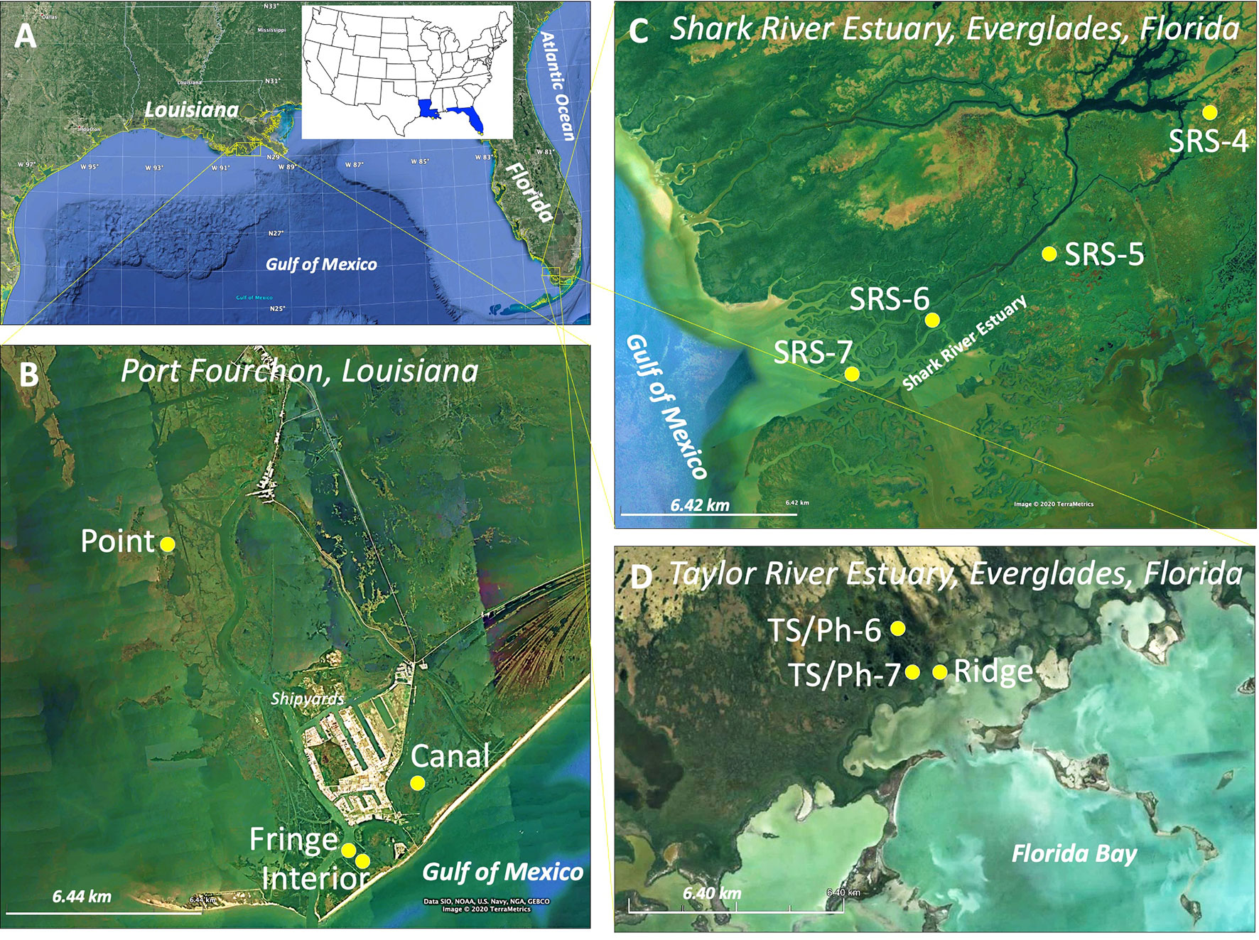
Figure 2 (A) Study sites in Port Fourchon (PF), coastal Louisiana and Florida Coastal Everglades (FCE), South Florida; and (B) Four mangrove-saltmarsh ecotone sites: Canal, Interior, Fringe, and Point in Port Fourchon; (C) Four riverine mangrove sites along the Shark River estuary (SRE) from upstream (SRS-4) to midstream (SRS-5), downstream (SRS-6), and estuary mouth (SRS-7); and (D) two scrub (TS/Ph-6 and TS/Ph-7) and one fringe (Ridge) mangrove sites at the Taylor River estuary (TRE).
The hydrology of Port Fourchon (PF) is driven by precipitation, the seasonal discharge of the Mississippi River distributaries, and wind-driven flushing of the bays, which is dominant across the Louisiana delta plain (Feng and Li, 2010; Li et al., 2011; Li et al., 2018; Xue et al., 2018; Zhang et al., 2022). In the Everglades, hydrology and hydroperiod are controlled by surface and groundwater flow in a karstic environment in the absence of rivers (Childers et al., 2006). Thus, nutrient and sediment availability is higher in coastal Louisiana than in South Florida; in the latter region, phosphorus is a limiting nutrient, and sediment transport is minimal from the upstream watershed into the coastal zone (Craig et al., 1979; Childers et al., 2006; Rivera-Monroy et al., 2011; Day et al., 2021). However, this pattern can be modified during the tropical cyclone season (June–November) when storm surges deposit resuspended sediments rich in phosphorus from the adjacent embayment and the continental shelf (Castañeda-Moya et al., 2010; Castañeda-Moya et al., 2020).
We selected four study sites near Port Fourchon; two sites are near the coastline (i.e., Interior and Canal), while the site Point is ~10 km northwest of those sites (Figure 2B). The dominant vegetation across all these three sites is saltmarshes (S. alterniflora) and A. germinans monospecific scrub mangroves (< 2 m). Although mangroves have been recorded in this region since the 1940s (Penfound and Hathaway, 1938; Osland et al., 2017), in the last three decades, they have been expanding into marsh habitats where mixed vegetation transition zones (i.e., ecotone) are apparent within each site. The fourth study site (Fringe), adjacent to the Interior site, is a monospecific A. germinans fringe forest with a mean tree height ranging from 3–4.5 m. The climate of this region is humid subtropical, with annual mean precipitation totaling 160 cm and a mean monthly temperature range of 6–30°C (Ghajarnia et al., 2020). The tidal regime is diurnal (typical maximum tidal range: 0.6 m) and is typical of the Mississippi River delta plain, which is impacted by one of the highest relative sea-level rise (RSLR) rates (9.13 ± 0.41 mm/year from 1947 to 2019 (Grand Isle, LA, NOAA station; https://tidesandcurrents.noaa.gov/sltrends/).
The study sites in the Florida Coastal Everglades (FCE) are a part of the Long-term Ecological Research (LTER) network established in 2000 in the Everglades, South Florida (Childers, 2006) (Figures 2C, D). The climate in this region is classified as tropical savanna with an annual mean precipitation of 150 cm and a mean monthly temperature range of 15–32°C (Abiy et al., 2019; Ghajarnia et al., 2020). Our riverine mangrove forest study sites along the Shark River estuary (SRE) are characterized by well-defined salinity and soil total phosphorus (TP) and hydroperiod gradients from the upstream (SRS-4) to the midstream (SRS-5) and downstream (SRS-6) regions and estuary mouth (SRS-7) (Figure 2C) (Castañeda-Moya et al., 2020; Zhao et al., 2021). Three dominant mangrove species (i.e., R. mangle, L. racemosa, A. germinans) in this region form mixed-species forests depending on the interaction among those environmental gradients, which determine complex trajectories in forest successional stage, tree height (range: > 6–18 m on average), and tree density (2838–7746 trees ha-1) from upstream to the estuary mouth (Castañeda-Moya et al., 2013; Simard et al., 2019). Three study sites are in the Taylor River estuary (TRE), north of Florida Bay (Figure 2D). This region is dominated by R. mangle (tree height: ~1–2 m) scrub mangrove forests due to the regulatory interaction of low soil TP, high sulfide concentration, and long inundation duration throughout the year (Castañeda-Moya et al., 2013; Hogan et al., 2021). These sites are specifically located upstream (TS/Ph-6) and downstream (TS/Ph-7) (Figure 2D) along the TRE. The third site is located on a natural levee in the TRE (Ridge), where hypersaline conditions (porewater salinity > 50 ppt) can develop during the dry season due to higher ground elevation compared to the other sites (Figure 2D). The dominant mangrove species in the Ridge site is A. germinans mixed with succulent herbaceous plants (e.g., Salicornia spp, Batis spp); tree height in this site is between 5–7 m. R. mangle, and L. racemosa are also present in this site at the edge of the levee where plants are flooded by semi-diurnal tides and freshwater discharge during peak precipitation events (Coronado-Molina et al., 2004; Michot et al., 2011).
2.2 Macroclimate Temperature Measured at Coastal and Inland Meteorological Stations
We compiled long-term (up to 70 years) TFree datasets recorded at inland and coastal meteorological stations on the Louisiana and South Florida coastlines. The closest stations to our study sites were selected to evaluate the regional temperature anomaly and determine potential temperature offsets at the air-vegetation canopy interfaces (Supplementary Figure S1). We compiled TFree data from the inland Galliano station (29.44°N, 90.26°W) and coastal Grand Isle station (29.25°N, 89.07°W), which are both less than 30 km from the Port Fourchon, Louisiana sites; in the case of the Florida sites, we used data from the inland Royal Palm (25.39°N, 80.06°W) and coastal Flamingo stations (25.14°N, 80.91°W), which are approximately 29 km from the Shark and Taylor River sites (Figure S1). We first used monthly TFree datasets reported for these four sites to assess the annual TFree anomaly. Over the last three decades (1990–2019), the TFree anomaly has increased in Louisiana and South Florida compared to the baseline average temperature from 1949–1989 (Figure S2). This warming trend was faster inland (Louisiana: slope = 0.037; Florida: 0.048) than in coastal areas (Louisiana: 0.011; Florida: 0.020). On average and during our study period (2017–2019), the overall variability of the anomaly was greater in South Florida (range: 0.87–1.92°C) than in coastal Louisiana (range: −0.085–1.28°C) regardless of whether the meteorological stations being compared are inland or near the coastline. These meteorological datasets are open access via the National Centers for Environmental Information (NCEI; https://www.ncdc.noaa.gov/cdo-web/).
Further, we used the TFree datasets reported for the coastal stations (Grand Isle, Louisiana; Flamingo, South Florida) to assess offsets of air-canopy temperature at each study site. These coastal TFree data represent the temperatures outside the vegetation coverage and account for the potential influence of adjacent coastal waters and winds in relative humidity and air temperature. Specifically, over the study period (2017-2019), the available TFree dataset reported for Grand Isle station (NOAA; https://tidesandcurrents.noaa.gov/) is on an hourly basis while for the Flamingo station is daily (NCEI; https://www.ncdc.noaa.gov/cdo-web/). Only this NOAA Grand Isle station TFree data are recorded at 3.9-meter height above local elevation while all other TFree data are at 1.5-meter height, following the National Weather Service Cooperative Observer Program guidelines (NWS COOP) (https://www.weather.gov/coop/standards).
2.3 Microclimate Temperature in Coastal Wetlands
We recorded in situ (microclimate) TSoil and TCanopy in all wetland sites using commercial waterproof sensors (Figure S3). TCanopy was measured using a temperature sensor (Onset HOBO UA001-08) protected from direct solar radiation using a standard shield (AcuRite, Chaney Instrument Co.). The shield is required to avoid the compounded influence of direct solar radiation and thus, the record is the actual ambient temperature under the vegetation canopy (Terando et al., 2017). This sensor set was deployed at ~50 cm above ground under the saltmarsh and scrub mangroves vegetation canopy (Figure S3); in the case of taller vegetation (i.e., > 2 m; fringe and riverine mangroves), the sensor was deployed at ~1.2 m above the ground. This height ensures a measurement near the so-called active surface–the imaginary plane of principal climatic activity within a canopy, with energy, mass, and momentum exchanges treated as if they originate or terminate at this plane. A TSoil sensor (Onset HOBO U22-001) was placed ~25 cm below the soil surface near the TCanopy sensor. Another sensor (Onset HOBO U22-001) was installed to detect water temperature (TWater) in the adjacent tidal creeks/embayment; this sensor was deployed at the middle-lower average water column depth to warrant permanent submersion. TCanopy, TSoil, and TWater were recorded hourly (one sample per hour). Because of logistical/sampling limitations (e.g., sensor loss or power failure), we collected data for ~3 years at the Louisiana sites and ~1 to > 2 years at the Florida sites; the overall observation period was from 2017 to 2019.
Here we define the offset as the temperature difference among the macroclimate (TFree) and the microclimate (i.e., TCanopy and TSoil) temperatures. Specifically, we define the canopy offset as the temperature difference between free-air and canopy-air temperature (TFree minus TCanopy), while the soil offset is the difference between canopy-air and soil temperature (TCanopy minus TSoil). We calculated offset values using daily mean temperatures.
2.4 Hydroperiod Measurements
To estimate frequency, duration, and depth of inundation in each study site, we measured in situ water level (WL) time series using ultrasonic WL recorders (INFINITIES USA, INC). The recorders were installed inland ~20–80 m from the adjacent tidal creeks/embayment at each study site. In the cases of Louisiana wetlands, a recorder was installed in both saltmarsh and scrub mangrove habitats in Interior and Canal sites; recorders were only installed in the mangrove habitat in the Point (scrub) and Fringe (fringe) study sites. The saltmarsh WL in the Point site was determined using the elevation difference (19.03 cm) between the adjacent scrub mangrove and the saltmarsh habitats. This elevation difference was obtained from an in situ topographic surveys conducted on July 28, 2017, using a GPS-RTK (Global Positioning System-Real Time Kinematic) system (Dr. Shelley Xuelian Meng, LSU, unpublished data). The WL recorder was placed on top of a PVC pipe (3-inch diameter; ~2.5-m length) buried ~1 m below the soil surface. WL relative to the soil surface was recorded hourly (one reading per hour). Thus, the below-ground PVC section registered the water table level in the absence of flooding (WL < 0) (Zhao et al., 2020). WL measurements used in this study were recorded simultaneously along with temperature (2017–2019). We used the average positive WL values (WL > 0) to determine the inundation depth above the soil surface.
To determine the relationship between in situ WL in wetlands and regional tidal regimes (hereafter channel-WL), we compiled available hourly WLs from long-term monitoring gauges near our study sites. These channel-WL datasets were collected and maintained by multiple agencies, including two NOAA stations (Port Fourchon: 29.1°N, 90.2°W; Grand Isle: 29.25°N, 89.95°W) near Louisiana study sites (https://tidesandcurrents.noaa.gov/). Similarly, five WL gauges were selected near Florida sites: three stations are part of the FCE-LTER monitoring stations network (https://fcelter.fiu.edu/data/) at Shark River sites (SRS-4, SRS-5, and SRS-6), while two stations are operated by the Everglades Depth Estimation Network (EDEN) (https://sofia.usgs.gov/eden/) at the Taylor sites. The EDEN sites are located upstream (25.21°N, 80.65°W; near TS/Ph-6) and at the mouth of Taylor River (25.19°N, 80.64°W; near TS/Ph-7 and Ridge).
2.5 Extreme Weather Events
Several weather events—cold fronts and tropical cyclones—occurred during the study period (2017–2019) in both regions (Figure S4). Not only can these events (i.e., hours) result in rapid temperature fluctuations, but also cause canopy defoliation and flooding that in turn modify the microclimate regimes, depending on the disturbance magnitude and duration. Due to its location, coastal Louisiana is seasonally impacted by frequent cold fronts (Li et al., 2019) compared to a lower frequency in South Florida (Ross et al., 2009; Danielson et al., 2017). In January 2018, several cold fronts induced significant mangrove canopy defoliation in the Louisiana mangrove habitats (Interior and Fringe sites; Figure S4). Thus, to evaluate the relative changes in temperatures driven by cold fronts in coastal Louisiana during this period, we examined the statistical relationship among TSoil, TCanopy, TWater, WL in wetlands and channels and other atmospheric variables (wind speed and air pressure). We determined the differences in temperature offsets between the pre-cold-front (the study period before January 2018: January–December 2017) vs. the post-cold-front (the study period after January 2018: February 2018–December 2019) periods in Louisiana to assess how microclimate regimes are affected by cold fronts over the long term.
Tropical cyclones seasonally impact both coastal Louisiana and South Florida (Smith et al., 2009; Holland et al., 2010; Castañeda-Moya et al., 2020; Zhao et al., 2021). The cyclone impacts are more visible in South Florida given the higher mangrove forest structural development in this region where tree heights can exceed 17 m (Danielson et al., 2017; Rivera-Monroy et al., 2019; Simard et al., 2019). This impact includes the formation of canopy gaps due to massive defoliation or tree fall, which allow more incident solar radiation to reach the soil surface, thus modifying the soil and canopy microclimate (Figure 1). In 2017, Hurricane Irma (Category 3) made landfall ~60–70 km from our Shark sites on September 10th. As a high-energy cyclone, Irma caused > 90% mangrove defoliation (Castañeda-Moya et al., 2020; Lagomasino et al., 2021; Zhao et al., 2021). Hence, we evaluated the relative magnitude in microclimate fluctuations of pre- and post-Irma impact in Florida sites.
2.6 Data Analysis
2.6.1 Cumulative Sum Graph
To evaluate the underlying time series features of temperature and WL datasets, we used CUmulative SUM (Cusum) plots to identify trends and rapid changes and visualize and quantify potential driver-response relationships (Briceno and Boyer, 2010). The Cusum is the cumulative sum of deviations from the overall mean against reference observations to remove high-frequency noise and smooth data series (Briceno and Boyer, 2010; Regier et al., 2019). Since the data are transformed into a cumulative response in this analysis, the interpretation of a Cusum plot is different from the standard time-series data graph. A segment with a positive slope in a Cusum graph indicates that the values in the original series are above average during a given period; correspondingly, the negative slope indicates that the values are below average; the horizontal segment in the graph thus represents the overall dataset average value (Regier et al., 2019).
2.6.2 Spectral and Wavelet Analysis
We applied spectral and wavelet analyses to assess how TSoil responds to variations in local hydroperiod and TCanopy and TWater. The spectral analysis was performed for the time series data using the Fast Fourier Transform (FFT). FFT is an efficient algorithm to obtain a Fourier transform; this is a mathematical method used to express temporal time series data in the frequency domain to quantify the variability at different frequencies (the spectrum). The wavelet analysis computes the power spectra as functions of time; it identifies and quantifies the event’s impact and temporal variation in the frequency domain. This analysis was performed to assess the coherence between TSoil and TCanopy, TWater, or WL, using the MATLAB software package (Grinsted et al., 2004). Wavelet analysis was also used to explore temperature and WL fluctuations associated with wind speed components and atmospheric pressure during cold front events. This method is commonly applied to explore time-dependent amplitude and phase for different frequencies in a time series, yet a significant coherence between two time series does not necessarily indicate correlation at high power. Before performing the spectrum and wavelet analyses, the Butterworth filter—which has favorable properties for problems with tidal signals (Li et al., 2011)—was used to separate the time series into low- and high-frequency signals. The cutoff frequency in this analysis was set to 0.6 cycles per day (cpd; equivalent to 40-hour cyclic period). Hence, we focused on analyzing high-pass time series with frequency > 0.6 cpd.
2.6.3 Statistical Analysis
We analyzed temperature offsets across different treatments represented by regional vegetation types (scrub, fringe, riverine mangroves, saltmarsh) in two coasts (Louisiana (LA), Florida (FL)), disturbance periods (pre- vs. post-cold-front or -Irma), months, and these treatments interactions. The site-specific vegetation types were: 1) scrub mangroves: Port Fourchon sites, LA (N=3; Interior, Canal, Point) and Taylor sites, FL (N=2; TS/Ph-6, TS/Ph-7); 2) fringe mangroves: Port Fourchon site, LA (N=1; Fringe) and Taylor site, FL (N=1; Ridge); 3) riverine mangroves: Shark sites, FL (N= 4; SRS-4, SRS-5, SRS-6, and SRS-7); and 4) saltmarshes: Port Fourchon sites, LA (N= 3; Interior, Canal, Point).
We performed an analysis of variance (ANOVA) for effects in two separate models (linear mixed-effect model and generalized least squares linear model) using the “nlme” statistical package in the R statistical framework (version 4.0.3; RStudio, 2020). To evaluate the overall differences among the six regional vegetation types (i.e., LA and FL scrub, LA and FL fringe, FL riverine mangroves, and LA saltmarshes), we considered the sites per coastal region (LA, FL) as replicates. Thus, we performed a linear mixed-effect model including the effects of regional vegetation types, periods, months, and their interactions along with a random factor (site), using the “lme” function. We also analyzed the temperature offset differences across site-specific vegetation types, periods, and months using generalized least squares to fit a linear model (“gls” function). The Tukey HSD post hoc comparison was performed using “emmeans” functions in the “emmeans” package (Lenth et al., 2018). Additionally, simple linear regressions were used to show how the hourly TSoil covaried with TCanopy and TWater, and to explore the relationships among hydroperiod components (frequency and depth). These linear regressions were performed using JMP® Pro 16 (SAS Institute Inc., Cary, NC, 1989-2021; Sall et al., 2017). The significance level used in all analyses was α = 0.05.
3 Results
3.1 Temperature Offset
While a positive canopy offset value indicates cooler conditions inside the wetland canopy-air, a negative value represents warmer conditions (Figure 3A). Overall, TCanopy exceeded TFree in all vegetation types except Florida riverine mangroves (Figure 3A). This offset significantly varied across regional vegetation types, periods, and months (ANOVA p-values < 0.05; Supplementary Table S1). Specifically, in coastal Louisiana and under pre-cold-front condition, the TCanopy in saltmarsh (–0.94 ± 0.08°C) and scrub mangroves (-0.89 ± 0.08°C) were significantly warmer than in the fringe mangrove (–0.19 ± 0.13°C), as indicated by the increasing canopy offset (Figure 3A). In post-cold-front conditions, the canopy offset in saltmarsh (–0.91 ± 0.07°C) increased slightly, while the offset in the scrub (–0.98 ± 0.07°C) and fringe (–0.48 ± 0.12°C) mangroves decreased when compared to the pre-cold-front conditions (Figure 3A). Only the decrease trend in fringe was significantly different from the case in the pre-cold-front period.
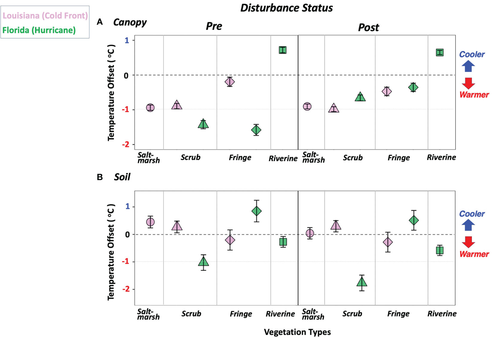
Figure 3 Least square means ( ± 1 SE) of (A) canopy offset (the difference between free-air and canopy-air temperatures) and (B) soil offset (the difference between canopy-air and soil temperatures) in the period of pre- and post-disturbance (i.e., cold front in Louisiana sites and Hurricane Irma in Florida sites) across multiple vegetation types, including saltmarsh, scrub, fringe, and riverine mangroves in wetlands located in coastal Louisiana and South Florida, respectively. Positive offset indicates cooler conditions while negative offset represents warmer conditions.
Similar to the patterns observed in the scrub mangrove in Louisiana, the scrub canopy air in Florida was warmer than free air with a significantly lower canopy offset value in pre-Irma (–1.43 ± 0.12°C) conditions than post-Irma (–0.66 ± 0.08°C) (Figure 3A). In the case of the fringe mangroves, the canopy air was warmer, as shown by the similar canopy offset value to the case of the scrub mangrove; this pattern was recorded in both pre-Irma (–1.58 ± 0.16°C) and post-Irma (–0.36 ± 0.12°C) periods (Figure 3A). In contrast, the riverine mangrove canopy air was cooler than free air; no significant difference in canopy offset was observed between pre- (0.72 ± 0.08°C) and post-Irma (0.65 ± 0.06°C) periods (Figure 3A).
Because the soil offset is the difference between canopy-air and soil temperature (TCanopy minus TSoil), positive values indicate that the soil is cooler than the canopy air and negative values represent a warmer soil status. The soil offset showed high variability (Figure 3B) and was characterized by significant differences across vegetation types, periods, and months (ANOVA p-values < 0.05; except for the interaction period*month, i.e., p = 0.2794; Table S1). In coastal Louisiana, the saltmarsh soil was cooler than the canopy air, yet the soil offset significantly decreased from the pre-cold-front (0.45 ± 0.22°C) to the post-cold-front (0.04 ± 0.21°C) period (Figure 3B). The soil in the scrub mangroves also remained cooler but changed within a narrower offset range than the one observed in the saltmarsh in both pre-cold-front (0.27 ± 0.21°C) and post-cold-front (0.30 ± 0.21°C) periods (Figure 3B). In contrast, the fringe soil was warmer with negative offset slightly decreasing from pre-cold-front (–0.20 ± 0.37°C) to post-cold-front (–0.28 ± 0.36°C) period.
TSoil in the Florida mangroves generally exceeded TCanopy except in the case of the fringe mangrove where the soil was cooler, as indicated by the positive soil offset (Figure 3B). Overall, the soil offset values showed similar pattern across the vegetation types in both pre- and post-Irma periods, increasing from the scrub to the riverine and fringe mangroves (Figure 3B). Specifically, the scrub mangrove soil offset (–1.03 ± 0.28°C; Taylor) was lower than the value in riverine (–0.27 ± 0.20°C; Shark) and fringe (0.85 ± 0.39°C; Ridge) mangroves during the pre-Irma period. In the post-Irma period, the offset values in scrub (–1.77 ± 0.29°C), riverine (–0.58 ± 0.19°C) and fringe (0.51 ± 0.36°C) mangroves decreased when compared to the values in the pre-Irma period. This decrease trend in soil offset values from pre-Irma to post-Irma was significant in both riverine and scrub mangroves. Mean value differences in temperature offsets per sampling site, vegetation type, and region, influenced by the disturbance periods (cold front, tropical cyclone) and month, were relatively similar (Figure S5).
3.2 Linear Relationships Between Soil and Canopy Air and Water Temperature
The linear regressions between hourly TCanopy vs. TSoil and TWater vs. TSoil for selected sites/vegetations and months (January, July, October, and December) showed significant hourly differences in TSoil on seasonal basis (Figures 4, 5; Tables S2, S3). The coefficient of determination between TCanopy and TSoil (R2 < 0.25) in winter (January and December) (Figure 4; Table S2) was lower than in the fall (October; R2 range: 0.24–0.49); the lowest value was registered in summer (July; R2 < 0.1) when the TSoil remained within a narrow range compared to a higher hourly variability in other seasons. Overall, the TWater accounted for > 45% of TSoil total variance during January, October, and December for all sites/vegetations in both Louisiana and Florida (R2 values; Figure 5; Table S3).
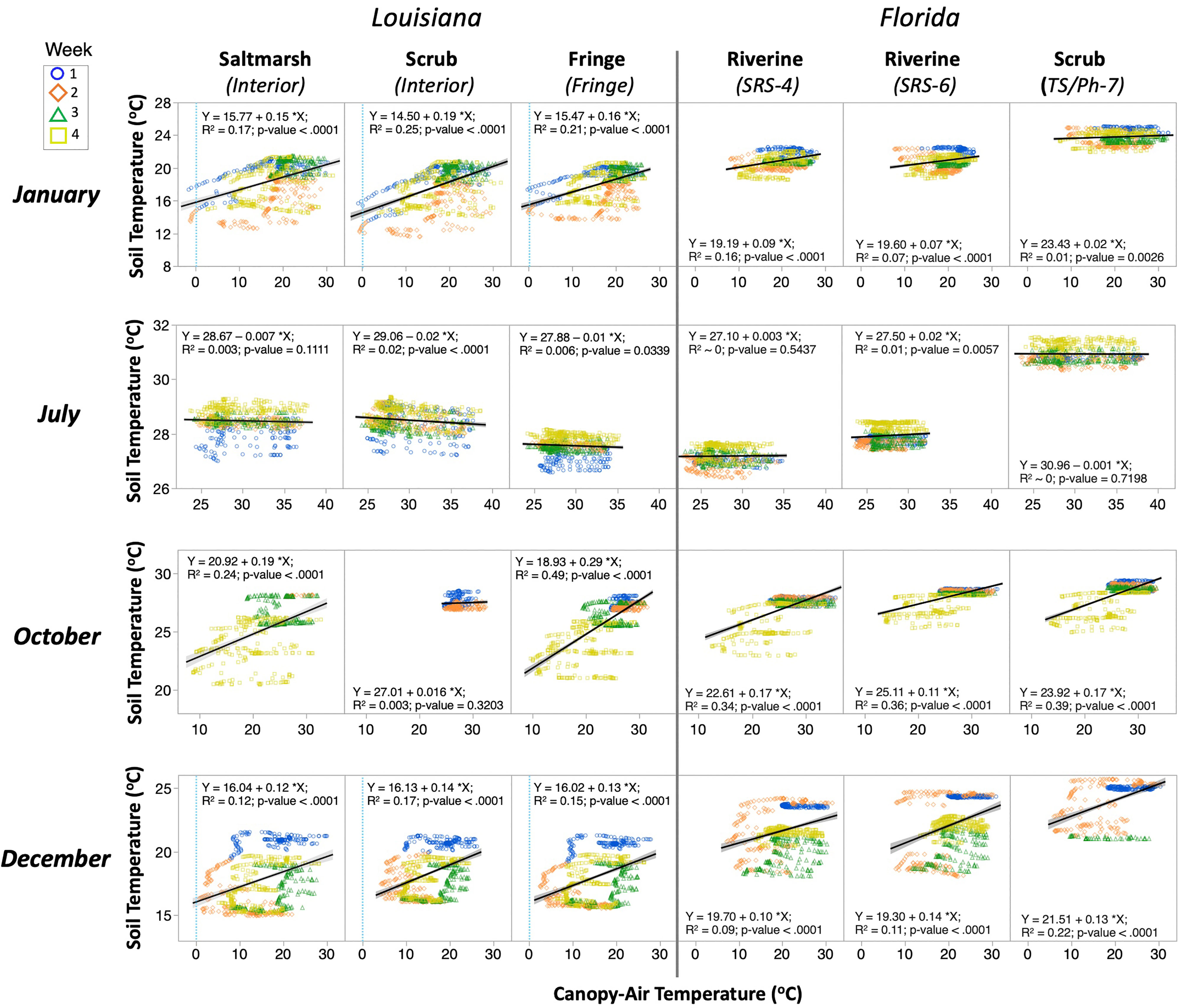
Figure 4 Linear regressions between hourly canopy-air and soil temperature recorded in selected wetland sites and months in 2017. The gray shade indicates the 95% confidence interval. The colored icons represent the week in a month when temperature was recorded. Notice the x- and y-axis scales are different among months. Light blue dashed lines mark the zero value in the winter months (January and December) in the Louisiana study sites.
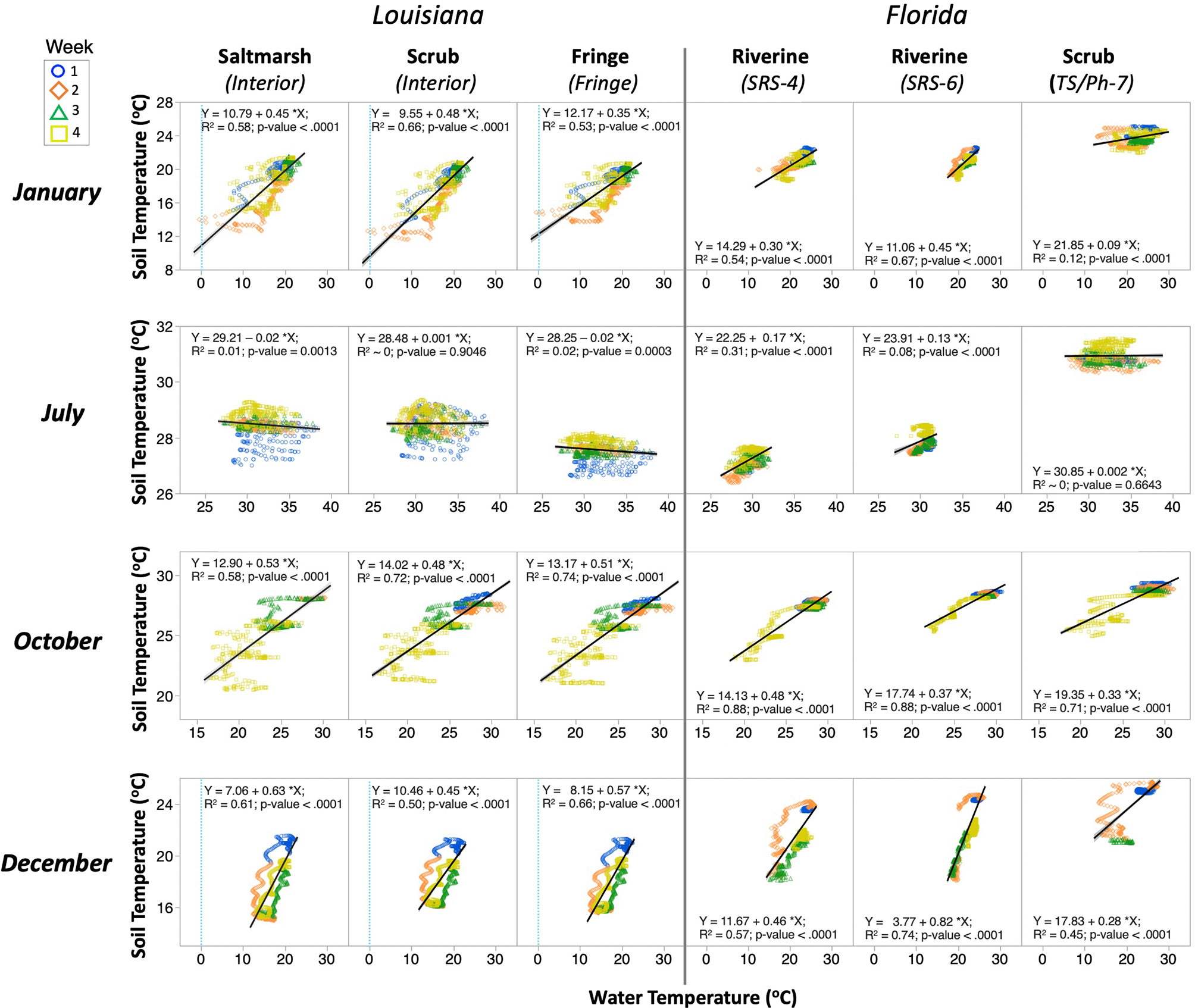
Figure 5 As in Figure 4, but for linear regressions between hourly water and soil temperature recorded in selected wetland sites and months in 2017.
These regression results underscore the high variation in TSoil in relation to TCanopy and TWater in different weeks within each month (Figures 4, 5; Tables S2, S3). This pattern provided information about the TSoil changes that are modulated by WL fluctuations associated with the local biweekly tidal variations (i.e., spring and neap tides) in each coastal region. The TCanopy vs. TSoil regressions, for instance in January 2017, showed a higher variability in the second and fourth weeks in the Louisiana sites, while these weekly differences were absent in Florida. One extreme case in this pattern was the decoupling at the air-water-soil interfaces through December at all sites (Figure 4). During the fall season (i.e., October), TSoil at the Louisiana sites showed greater variability in the fourth week than at the Florida sites (Figure 4). During summer (i.e., July), the regressions were weak in all sites (horizontal lines); the greatest data dispersion in this flat pattern was observed in the first and fourth week in the Louisiana sites. Yet, the data variability showed in the TWater vs. TSoil regressions was significantly smaller than that between TCanopy and TSoil (Figure 5), thus underscoring the high interaction in heat transfer/regulation between the soil and the overlying water.
3.3 Hydroperiod Spatiotemporal Patterns
The WL measured at each site was variable across regions given the different tidal regimes along the nGoM as well as the seasonal variations in weather. The spectral analysis showed that coastal Louisiana was dominated by diurnal tides while the Florida Shark sites have a semi-diurnal tidal regime (Figure S6). Although the wetlands and adjacent water column (channel-WL) had the same tidal constituents, the tidal signal had higher power in the channel-WL than in the wetland. The WL in the Louisiana wetlands had relatively higher power at the diurnal (1 cpd) band, which was aligned with the peak value monitored at the two NOAA stations (Figure S6A, B). In the South Florida sites, the channel-WL picked up 1- and 2-cpd bands and showed a higher power at 2-cpd band, except at site SRS-5, where higher power was identified at 1-cpd band (Figure S6C, D). The tidal signal in the Taylor sites was generally absent and weather effect was dominant. This pattern was due to the location of Taylor sites, which are behind natural levees that limited tidal exchange between the Taylor River and Florida Bay (Figures 2C, D).
The duration and frequency of inundation differed across vegetation types and coastal regions while inundation depth was within a close range (Figure 6; Table S4). The range in monthly inundation depth (10–40 cm) was similar among those water levels recorded in the Louisiana Interior and Point saltmarsh (Figure 6A, C) and the Florida Taylor scrub mangroves (Figures 6L, M). Yet, the frequency of inundation range (e.g., number of flooding events per month; i.e., events month-1) was relatively narrow and decreased from the Interior (~1–40 events month-1) and Point (~1–20) saltmarshes. The Canal saltmarsh (Figure 6B) had a monthly water depth (< 20 cm) and frequency (~1–60 events month-1) near the values registered in the Louisiana scrub mangroves (Figures 6D–F). The mean water depths in mangroves along the SRE and at the Ridge site were < 20 cm (Figures 6H–K, N). There were two distinct frequency values registered at the site SRS-7 (~40–70 events month-1), located near the SRE mouth, and the fringe mangrove in the Ridge site (~1–30 events month-1) (Figures 6K, N). The inundation duration in the Interior and Point (~400–> 700 hours month-1) sites in coastal Louisiana was longer in the saltmarshes than in scrub and fringe mangroves (~50–> 600 hours month-1); these values were similar to values registered in the Taylor scrub mangroves in Florida that are permanently flooded throughout the year (frequency < 10 events month-1; duration > 700 hours month-1).
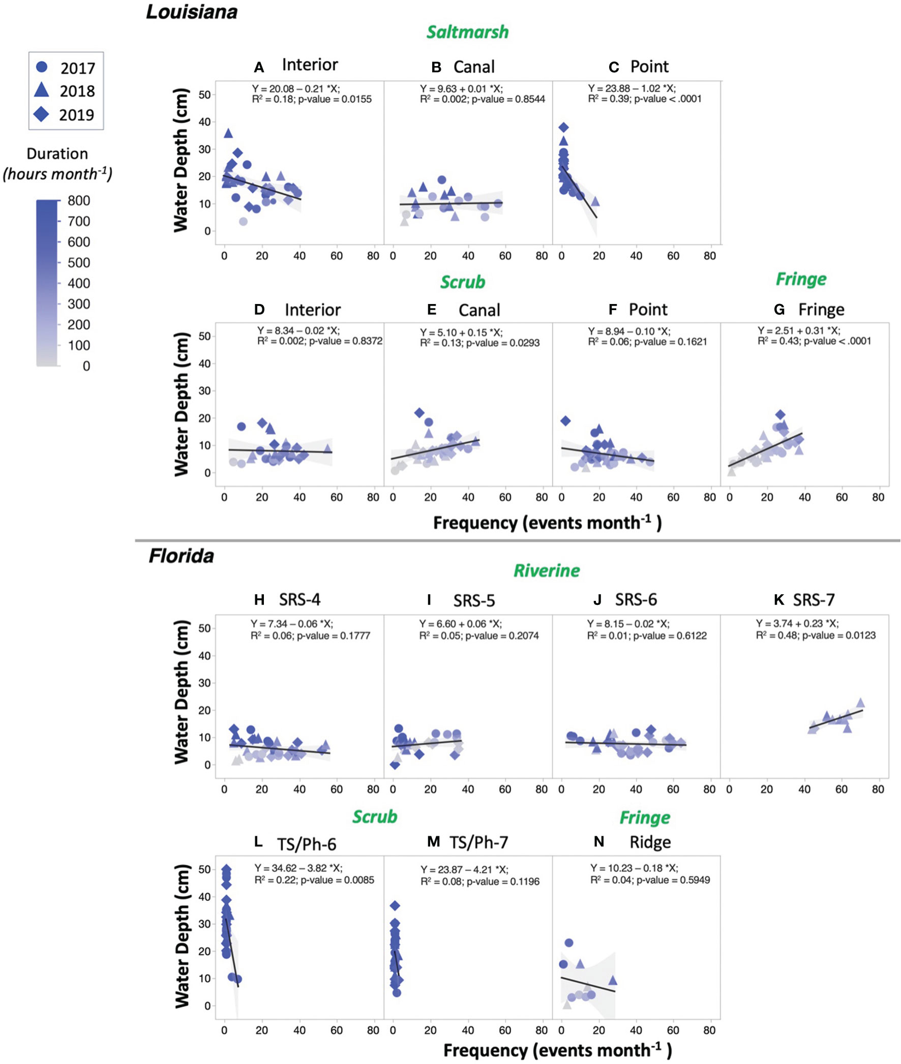
Figure 6 Monthly hydroperiod gradients across vegetation types and sites summarized based on in situ water levels collected in wetlands from year 2017 to 2019. Linear regressions were performed between monthly frequency of inundation (count of flooding events in a month; events month-1) and flooding water depth (average of positive water level when the wetlands are flooded; cm). The gradient blue color represents the monthly duration of inundation (total flooding hours in a month; hours month-1). The gray shade indicates the 95% confidence interval.
3.4 Soil Temperature Modulated by Water Temperature and Water Level
TCanopy and TWater showed a similar trend on hourly basis, with higher fluctuation/range in the TCanopy during the day relative to TWater. Yet, TSoil showed less variation and was relatively stable within a narrow range (< 2–8°C) when compared to TCanopy and TWater (10–> 20°C) and depending on the season (Figures 7, 8). TSoil was generally near or greater than TCanopy and TWater in winter (i.e., January and December), especially during the occurrence of cold fronts. The TSoil was cooler than TCanopy and TWater in summer (i.e., July) and with an opposite response under warmer conditions during the fall transition (October) when regional macroclimate temperature became colder. These high covariations among TCanopy, TSoil, and TWater were also apparent in the Cusum graphs (Figure S7). Moreover, the TSoil was closely associated with WL changes, as also shown by the similar seasonal Cusum patterns across coastal regions. The temperature spectral analysis showed that all temperatures (canopy-air, soil, water) had a common peak in the diurnal cycle (1 cpd) that is driven by solar radiation (Figure S6E, F). TCanopy also peaked at the semi-diurnal cycle (2 cpd) but at a lower power value compared to the diurnal cycle power—although this peak disappeared in the case of the TSoil and TWater signals.
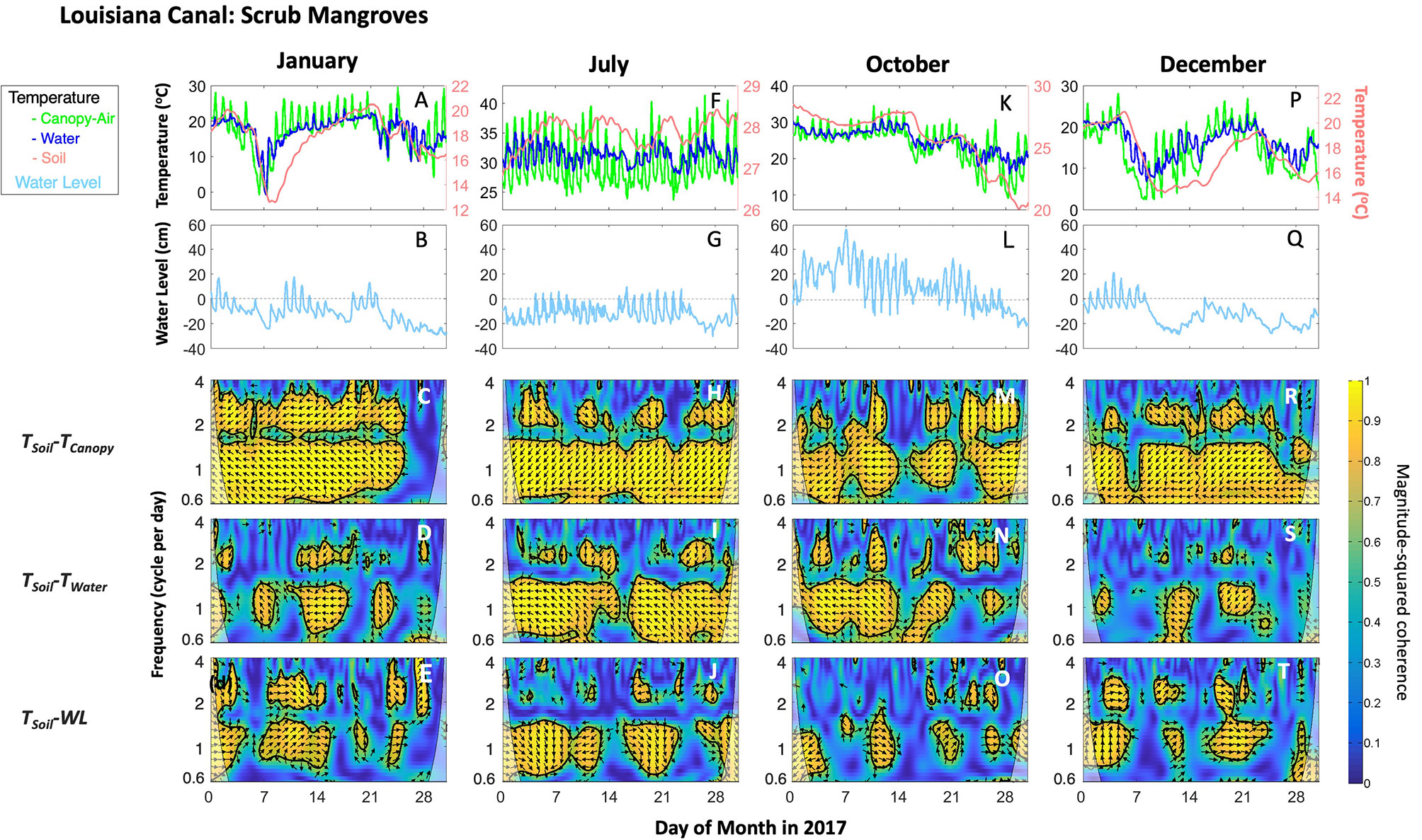
Figure 7 Temperatures in three mediums (row 1: A, F, K, P; i.e., Canopy air: TCanopy, Soil: TSoil, and Water: TWater), water level (WL; row 2: B, G, L, Q), and wavelet plots (rows 3−5; frequency in cycle per day or cpd) for scrub mangroves in the Canal site in Port Fourchon, Louisiana during 2017. Selected months represent different seasons. The wavelet coherence values are displayed for paired TSoil-TCanopy (C, H, M, R); TSoil-TWater (D, I, N, S) and TSoil-WL (E, J, O, T). The colored wavelet panels (blue to yellow tones) show the wavelet magnitude-squared coherence. The arrow direction indicates the phase difference between the pair of variables: a right direction indicates that the variables are in phase while a left direction indicates that the variables are out of phase. Yellow areas bounded by thick black lines indicate significant coherence at the 95% level. Notice that the soil temperature (row 1) is shown in red color along the right-side y-axis scale.
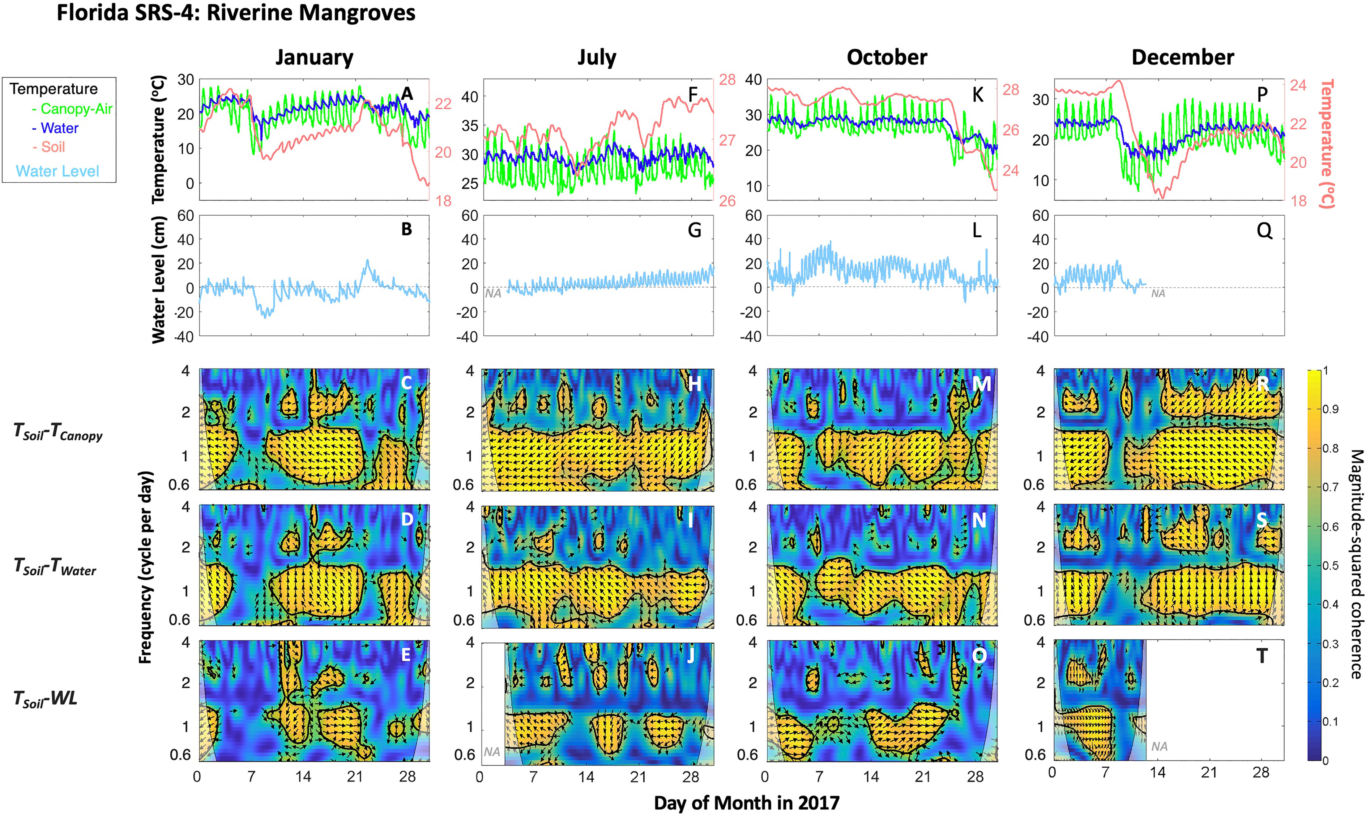
Figure 8 As in Figure 7, but for riverine mangroves at SRS-4, Shark River estuary, Florida Coastal Everglades, South Florida during 2017. “NA” indicates data were not available due to the limited sensor memory or power failure.
The wavelet coherence among different combinations of TSoil, TCanopy, TWater and WL is shown for selected months in the case of mangroves in the Canal (Louisiana) and SRS-4 (Florida) sites (Figures 7, 8) given the difference in the range of temperature. Similar results were found for other sites (data not shown). Overall, TSoil was coherent with TCanopy, TWater, and WL at a common 0.6- to 2-cpd band. The paired TSoil-TCanopy coherence was generally significantly persistent at 1-cpd over a month. TSoil and TWater (or WL) also covaried at 1-cpd band; but the paired TSoil-WL suggests an overall patched power at this specific band (Figures 7, 8).
The anti-phase arrows (arrows to the left) located within a significant range indicate that the TCanopy and TWater fluctuations drive TSoil fluctuations. During winter (i.e., January, Figures 7A–E; December, 7P–T) at the Louisiana sites, the observed coherence of the paired TSoil-TCanopy at the 0.6- to 1-cpd band persisted throughout the months, except in periods when temperature decreased along with low WL occurring in the 25–30 days in January and days 5–7 and 25–31 in December 2017. Further, the power for the paired TSoil-TWater and TSoil-WL was significant or relatively higher at the 1- or 2-cpd band during a cold frontal event. Similarly, in the fall (i.e., October; Figures 7K–O) the coherence of the paired TSoil-TWater and TSoil-WL showed significant power during cold frontal events (days 15 and 22) when a significant coherence was absent between TSoil and TCanopy. This significant coherence pattern was also observed in a cold frontal event occurring in the second week of January (Figure 7A). In addition to the observed patterns during the cold frontal event, TSoil under high flooding conditions was also significantly connected to TWater and WL at 1- or 2-cpd band when TCanopy and TWater were relatively stable during January (days 16–20), October (days 1–14) and December (days 1–3; 16–22). During summer (i.e., July; Figures 7F–J), the relatively high WL at the soil subsurface (water saturated soil) driven by the high tide phase played a vital role in maintaining the relative TSoil stability within a narrow range (~26.5–28.5°C) while TWater fluctuated from 25–35°C (Figures 5, 7F). The coherence between TSoil and TWater or WL was also persistent at 0.6- to 1-cpd band, except around days 15 and 25 when WL was relatively lower due to the neap tide (Figures 7F, G).
The temperature values were higher within a narrow annual range in the Florida sites; the paired temperature coherence showed a similar pattern throughout the year (Figure 8). Although we did not detect a significant coherence between TSoil and WL when temperature decreased (e.g., days 5–10 in January, days 25–31 in October, and days 7–10 in December) (Figures 8A, K, P), the coherence pattern in other days were significant due to the relatively high WL. Further, paired TSoil-TWater showed relatively high power at 1-cpd band in these days despite the power being outside a significant range boundary (Figures 8D, N, S). During summer, the paired TSoil-TWater coherence (Figure 8I) was persistent over the month scale while the paired TSoil-WL (Figure 8J) showed a patchy significant power as TSoil changed over time; this indicates the soil buffering capacity in maintaining its temperature—and heat content—as WL fluctuates at different temporal scales.
3.5 The Relative Role of Extreme Weather Events in Altering Microclimate in Coastal Wetlands
Due to the differences in latitudinal location, the Louisiana sites were more impacted by cold fronts in contrast to the South Florida region during the study period. The lowest TFree value was registered during the passage of a cold front on 17 January 2018 (–4.6°C at Grand Isle NOAA station) (Figure S8). During this event, the TCanopy ranged from –5 to –4°C while the TSoil maintained a temperature > 10°C (data not shown) across Louisiana sites. A wavelet analysis underscored this decoupling using hourly time-series measured in the scrub mangroves in the Louisiana sites during the cold front (e.g., Canal site; Figure S9). Here, the wavelet coherence among temperatures and WL time series were similar to the pattern observed in winter 2017 (Figures 7C–E). In particular, the paired TSoil-TCanopy and TSoil-TWater coherences were persistent at 1-cpd band while the paired TSoil-WL significantly covaried at 1-cpd band only when the temperature decreased during cold fronts: days 1–6 (c1), days 11–14 (c2), days 15–18 (c3), days 23–25 (c4), and days 28–30 (c5) (Figures S8, S9); a significant patchy coherence was also detected at the 2-cpd band during these sequential cold events.
The cold fronts impacted WL in both the channel and inside the wetlands. The paired wind speed spectrum, either of the NS or EW wind component, and that of the WL (wetland or channel) time series exhibited connections that were evident in the observed fragmented pattern at the 1- to 2-cpd band (Figure S10). The common coherence was more evident at < 1-cpd band in the WL vs. NS wind spectrum and at the 2-cpd band in WL vs. ES wind spectrum.
4 Discussion
Our study revealed that the canopy offset between TFree and TCanopy in coastal Louisiana and Florida represents a significant buffering effect by the wetland vegetation canopy—a thermal mechanism also observed in terrestrial ecosystems (De Frenne et al., 2019; Zellweger et al., 2020). The absolute canopy offset range (~0.2–1.6°C; Figure 3) encompasses the magnitude of the regional/TFree anomaly estimated in the same period (2017–2019) in coastal Louisiana (range: –0.085–1.28°C) and in South Florida (range: 0.87–1.92°C) when using temperature data from 1949–1989 as a baseline (Figure S2).
This agreement in temperature offsets at the regional scale quantitatively highlights the role of vegetation in regulating vertical (0–20 m) energy fluxes in coastal wetlands. Spatially, the canopy offset across vegetation types and seasons was similar across regions, thus indicating the differential and functional role of the canopy density and extension in regulating the propagation of TFree anomalies into the marsh and forested wetland canopies (Figure 1). Our results highlight how this temperature offset can vary depending on the type of wetlands, especially in forested wetlands (i.e., mangroves) where variable canopy height can influence the magnitude and temporal variability of the air temperature offset, depending on the initial forest structure (e.g., tree height) and magnitude of disturbance (e.g., defoliation caused by cold fronts or tropical cyclones).
Overall, the average inundation depth (< ~20–40 cm) observed in both saltmarsh and mangrove habitats did not directly influence TSoil. The interaction between frequency and duration of inundation, however, had a significant effect on TSoil; the presence of water on submerged or semi-submerged soil buffers any short- and long-term increase or decrease in air temperature (e.g., TCanopy or TFree). This is equivalent to the role of the vegetation canopy in attenuating changes in free air but under different heat flux regimes and chemical and stoichiometric composition among air, water, and soil. Indeed, our TSoil measurements at different temporal scales (hour, day, week, month) show not only significant fluctuations in the TSoil value but also in the offset range when compared to TCanopy and TWater.
Because the magnitude of this soil offset—regulated by the local frequency and duration of inundation—the hydroperiod must be explicitly considered when quantifying the long-term relationship between TSoil and functional wetland ecosystem properties (e.g., organic matter decomposition, mineralization rates). Our results also underscore the short- and long-term impact of pulsing disturbances—especially the frequency of cold fronts in Louisiana—on temperature regimes at each wetland interface (free-air vs. canopy-air; canopy-air vs. soil; soil vs. water). Below we further discuss specific spatiotemporal patterns and temperature offset commonalities and differences between coastal regions.
4.1 Canopy Offset Between Free Air and Canopy Air
We found that the tall canopy in riverine mangroves along the Shark sites (SRE, Florida) promoted cooler conditions (i.e., positive canopy offset) when compared to the free air (i.e., TFree). This difference is partially driven by the highest tree stature range > 6–18 m (Castañeda-Moya et al., 2013) in this region compared to shorter stature (average < 2–3 m) at the Taylor sites (Coronado-Molina et al., 2004). At the Shark sites, the dominance of taller trees, associated with lower tree density, provides space under the forest canopy to allow an efficient air advection and mixing (Bramer et al., 2018; Zellweger et al., 2019). This well-mixed air promotes horizontal and vertical energy advection near the soil surface, thus cooling the canopy air. In contrast, the air mixture under low-stature scrub mangroves and saltmarsh is restricted due to the relatively denser stems/branches closer to the ground, thus leading to localized warmer canopy air than free air.
Although the Louisiana vegetation canopy height differences (range: 0.5–3 m) are relatively smaller than in the Florida sites (> 3 m), the mangrove and saltmarsh sites in coastal Louisiana also show similar canopy offset patterns; even when the offset magnitude was smaller. In this case, the canopy near ground becomes denser from the fringe mangrove site to the scrub mangroves and saltmarshes. Here, the warmer conditions are amplified and driven by a denser canopy as a response to changes in TFree (Figure 3A; Figure S5A). Thus, the air under the canopy in Louisiana fringe mangroves is relatively cooler given the well-mixed air mass, as is the case in the Florida Shark riverine mangroves. Because the fringe mangrove boundary is separated by ~5 m relative to the scrub mangroves and saltmarsh habitats in the Interior site (Figure 2B), we were able to assess the change in the canopy offset in the same location. This vegetation distribution illustrates how vegetation mosaics characterized by different vegetation structure can significantly change both TCanopy and TSoil within small spatial scales (~10 m × 10 m; Figure 2B) (Chen et al., 1999; Maclean et al., 2017).
Our findings further highlight the need to measure the interaction between ecological and physical processes (e.g., energy budget) at local scales to reduce uncertainty when modeling the microclimate in coastal areas. In these areas, ecotones are under habitat shifts as a result of dynamic changes in environmental gradients and geomorphology driven by natural processes and human impacts under a changing climate (Osland et al., 2018; Jucker et al., 2020; De Frenne et al., 2021). Explicitly, incorporating these temperature differences may improve both regional statistical models and ESMs, which are commonly developed from datasets at larger spatial scales (> 1–500 km) (Potter et al., 2013; Gabler et al., 2017; Alber and O'Connell, 2019; Ward et al., 2020). For example, one major uncertainty is the role of time lags of vertical (air, canopy, soil) temperature changes to enhance forecasting of coastal wetland vegetation shifts after pressing (i.e., climate change) and pulsing (e.g., freezes, hurricanes) events (Barr et al., 2012; Hardwick et al., 2015; Danielson et al., 2017; Zellweger et al., 2020). Similarly, hydroperiod can ameliorate changes in vegetation since a stable TSoil can promote faster vegetation recovery (Osland et al., 2015; Devaney et al., 2017; Osland et al., 2019) (see below).
4.2 Soil Temperature Modulated by Hydroperiod
The significant spatiotemporal variations in hydroperiod in both coastal regions were due to differences in the interaction between local topography and distinct tidal regimes (diurnal, Louisiana; semi-diurnal, Florida; Figure S6) (Nuttle, 1997; Li et al., 2018; Zhao et al., 2020). This difference was detected within the same region, thus affecting TSoil values (Figures 3, 6). For example, although we measured a similar canopy offset in the Louisiana scrub mangroves, the TSoil cooled after an increase in the soil offset gradient from the Interior and Canal to Point site (Figure S5B). This “within” site comparison shows that as the duration of inundation increases, an increase in heat exchange occurs resulting in a higher correlation between TSoil and TWater (Figure 5). This interaction thus reduces the TSoil value and promotes cooler soil conditions as the flooding duration increases in the scrub mangroves (Figures 6D–F). Similarly, in Louisiana saltmarshes, the soil offset also increases across saltmarsh sites as inundation duration increases (Figures 6A–C; Figure S5B).
The regulatory effect of hydroperiod on TSoil is compounded when comparing short-stature grasses (saltmarsh) and scrub mangroves vs. tall forests (riverine mangroves) owing to differences in vegetation height. In Florida riverine mangroves, which are under similar cooler TCanopy conditions (Figure S5B), the observed increasing TSoil trend across the Shark sites could be attributed to prolonged flooding conditions (water presence on top of the soil or groundwater saturating the soil) as a result of complex interaction between inundation frequency and duration along the SRE (Figures 6H–K) (Castañeda-Moya et al., 2013; Zhao et al., 2020). This is also reflected on the close association between the TSoil and TWater (Figure 5; Table S3). In the Taylor scrub mangroves, the TSoil values remain relatively high because of almost permanent flooding conditions as indicated by the warmer air temperature regime throughout the year (Figures 6L, M).
The water presence on top of the soil is equivalent to the role of ice or snow coverage in ecosystems located at higher latitudes (Parton et al., 1998; De Frenne et al., 2021). Depending on the flooding duration, for instance, the microclimate is modified by overlying water since it reflects more incident solar radiation compared to non-flooding conditions when the soil absorbs more heat (Figure 1B) (Barr et al., 2012; De Frenne et al., 2021). Moreover, the inundation regime can have a wide range of impacts in wetlands, depending on the local hydroperiod. Even when inundation duration is short and the overlying water column is shallow (< 2 cm), groundwater can saturate the soil and ameliorate TSoil changes relative to wider TCanopy and TFree fluctuations throughout the year. This pattern was observed during cold frontal passages in Louisiana (Figure 7). In January 2017, for instance, TSoil decreased following a sharp decline in the TCanopy and TWater in the Louisiana sites during the second and fourth week. Simultaneously, the WL was lower because of high air pressure that interacted with an ongoing neap tide that restricted flooding conditions; this interaction in turn affected the water saturation status of the surface soil layer. Although in this case the soil ground was exposed to low air temperature due to low WL, the coherence between TSoil and the WL or TWater was enhanced as indicated by the high coherence of paired TSoil-WL and TSoil-TWater (Figures 7A–E). A similar variation also occurred during other cold front events causing significant changes in temperature in the fall and winter seasons (e.g., fourth week in October and December) (Figure 7).
4.3 Cold Fronts and Tropical Cyclones as Pulsing Microclimate Drivers
The occurrence of low temperature at the regional scale impacts the microclimatic regime, in coastal wetlands as illustrated by the frequency and duration of cold fronts (Figures S4, S8). Strong winds associated with these extreme events may alter the above- and below-canopy airflows and near-ground energy fluxes. This alteration can lead to sudden changes in microclimate temperature under the vegetation canopy as indicated by the coherence analysis (Figure S10). The common coherence patterns show that the WL fluctuation is related to a wind pattern shift (i.e., speed and direction). Thus, the WL in wetlands driven by tidal oscillations—and sometimes influenced by a strong wind—can in turn modulate the TSoil magnitude and its daily or seasonal variability. Additionally, during cold fronts, the vegetation canopy can protect seedlings and propagules from freeze damage, thus preserving a potential seed/propagule bank for post-disturbance regeneration (Devaney et al., 2017). Moreover, because the hydroperiod can be temporally altered due to storm surge caused by cold fronts or cyclones, high WL inside the wetlands not only protects low-stature vegetation and seedlings but also minimizes direct damage during freezing or strong wind conditions (Osland et al., 2019; Armitage et al., 2020). These multiple direct and indirect effects regulating changes in hydroperiod can accelerate vegetation resprouting—as is the case of the species A. germinans—or reproductive output after disturbances, thus enhancing resilience and shortening vegetation recovery time (Osland et al., 2015; Chen et al., 2017; Danielson et al., 2017; Osland et al., 2019).
In addition to those immediate, and sometimes subtle impacts, there are also more severe, visible impacts including canopy defoliation and tree fall/mortality (Lugo, 2008). These impacts create canopy gaps in forested wetlands, allowing more incident radiation to reach the understory and soil surface, thus altering the microclimate in the short- (weeks) or long- (annual-decadal) term (Figure 1) (Doyle et al., 1995; Barr et al., 2012; Danielson et al., 2017; Osland et al., 2019; Rivera-Monroy et al., 2019). In coastal Louisiana, for example, the Interior scrub and Fringe mangrove sites were defoliated due to a cold front in January 2018. This frontal impact on the canopy was manifested as a slight decrease in the canopy offset, suggesting a reduction in the role of the canopy as a buffer (Figure 3A). This reduction in the canopy buffering capacity also occurred in the Shark sites due to Hurricane Irma’s impact in 2017. For example, in the post-Irma period, a lower canopy offset value was conspicuous in the SRS-6 site due to the massive (> 90%) defoliation (Figures S4, S5) (Castañeda-Moya et al., 2020; Zhao et al., 2021). However, the overall soil offsets during pre- vs. post-disturbances in both regions were not significantly different (Table S1). This is partially explained by the local spatial variability in canopy offset as the inter-annual macroclimate variations can balance the observed absolute reduction by the vegetation canopy (Figure S2).
Additionally, the same type of disturbance can have different degrees of impact. Another study assessing vertical changes in water vapor and CO2 exchange (eddy covariance) in the SRS-6 site before and after Hurricane Wilma’s (Category 3) impact in 2005 found significant changes in the difference between TFree and TCanopy (canopy offset) (Barr et al., 2012). This finding was partially attributed to the reduced canopy albedo one year after Wilma’s passage due to canopy defoliation (> 90%). Like our study, this temporal canopy loss also increased TSoil down to 50-cm depth (~1–2°C in 2007). In this case, the impact of both Hurricanes Wilma and Irma on mangrove forest structure along the SRE was relatively different due to the cyclone trajectory and distance from the SRS-6 site (Zhao et al., 2021).
Due to Hurricane Irma’s trajectory and mangrove tree stature (< 3 m) in the Taylor sites, we did not observe canopy defoliation (Castañeda-Moya et al., 2020). However, we registered an increase in the canopy offset (i.e., cooling). We suggest that this increase is related to the mangrove canopy response to warmer TFree in this coastal region as indicated by the greater post-Irma air temperature anomaly (1.38°C) when compared to pre-Irma conditions (0.87°C) (Figure S2) (De Frenne et al., 2019). It is difficult, however, to attribute this canopy offset change observed in Taylor scrub mangroves to a single factor because this area is characterized by a complex landscape where a mix of shallow ponds of variable extension and channels/tidal creeks are hydrologically interconnected by seasonal precipitation, upland runoff, wind, and groundwater (Sutula et al., 2001; Michot et al., 2011). Given the larger water surface that surrounds the mangroves in this area (Figure 2D), it is expected that water storage will exert a significant effect on local heat exchanges between the ponds/channel surface and the lower atmosphere; these exchanges, in turn, affect temperature patterns at different spatial scales. How these convective and advective air fluxes affect temperature and heat exchange between the vegetation and ponds/channels is not well understood, especially in areas where scrub mangroves are influenced by long duration of inundation (Figure 1, Figures 6L, M) (Schedlbauer et al., 2010; Malone et al., 2016).
This complex pattern underscores the non-linear responses of wetland canopy offset to macroclimate changes as a result of integrated impacts of interannual macroclimate variability, canopy density status, and hydroperiod; this is apparent in the Taylor region as reflected by the TSoil cooling trend in both the Taylor scrub and Ridge sites after the passage of Hurricane Irma (Figure 3A) (Feher et al., 2017; De Frenne et al., 2021). Although the disturbed mangrove canopy can recover in < 1 or > 4–5 years (Osland et al., 2015; Chen et al., 2017; Danielson et al., 2017), it is critical to incorporate the disturbance-induced cumulative variations in temperature offset to improve the large spatial extent/resolution simulations in GCM-ESMs, which is usually performed over a longer period (e.g., decade to century).
Regardless of temporal macroclimatic temperature differences between Louisiana and Florida’s inland and coastal sites, there is an unequivocal warming trend (Figure S2). This TFree increase can not only drive changes in local-scale coastal wetland offsets at different interfaces (e.g., canopy-water-soil), but also impact the frequency and duration of disturbances, including cold fronts and tropical cyclones. The synergy of these disturbances can determine the magnitude of the impacts on wetlands structure (e.g., height) and distribution and function, including canopy turnover rates affecting NPP and carbon export (Osland et al., 2020a; Zhao et al., 2021). Moreover, this warming trend further confirms the undergoing tropicalization of the nGoM as indicated by the continuing expansion of mangroves into saltmarshes due to less frequent freezing events (Cavanaugh et al., 2019; Osland et al., 2019). However, the net mangrove expansion needs to be evaluated while considering other drivers. For example, mangrove expansion in coastal Louisiana is now negatively affected by increasing erosion due to a lack of sediment deposition and high subsidence rates along with their combined impact with increasing relative sea-level rise (RSLR) that further compounds land loss (Giri and Long, 2016; Mariotti, 2020). The increasing erosion is observed in saltmarsh and mangrove habitats and reflected by current changes in soil offset values (cooling TSoil) at the Louisiana Point site. This overall decrease in TSoil is driven by an increase in flood duration during the last two years as wetlands are subsiding amid the lack of river sediment inputs (Couvillion et al., 2016).
4.4 The Need to Overcome Limitations in Upscaling Microclimate Temperature Patterns
Currently, the ESMs use macroclimatic temperatures recorded by regional meteorological stations or coupled to GCMs to initialize and drive numerical modeling experiments (Kay et al., 2015). A temperature-related parameter (Q10, temperature sensitivity) in these global models is usually included to simulate biogeochemical processes in soil or water under different temperature scenarios (Davidson and Janssens, 2006). In contrast to the Q10 parameter indirectly representing the effect of regional temperature regimes, in our study, we directly measure representative “single-point” temperature values at canopy height (~0.5 m or 1.2 m aboveground) and belowground (~25 cm) on seasonal and interannual frequencies. Yet it is still necessary to spatially expand these measurements to determine the in situ temperature variance (uncertainty) at a higher spatial resolution. These additional measurements can not only improve offsets estimates across the canopy-water-soil interface but also can be combined with other mesoscale functional vegetation properties such as leaf area index (LAI; Figure 1) to calibrate remote sensing models (Alber and O'Connell, 2019). This type of relationship can also help develop statistical models that can link vegetation structure (e.g., tree height, density) with in situ interface temperature measurements as an upscaling strategy.
Although current ESMs do not explicitly include coastal regions (Bonan and Doney, 2018; Ward et al., 2020), our study highlights the need to accelerate this inclusion to couple coastal hydrology and hydrodynamics and its interaction with specific landforms (e.g., deltas, coastal lagoons) at local and regional scales; especially the critical role of hydroperiod driving TSoil regimes in wetlands, as we found in coastal Louisiana and Florida (Figure 1). Explicitly adding the coastal processes in the ESMs will reduce model projection uncertainties and help determine how current and future TFree anomalies propagate into direct alterations in biogeochemical transformations and soil formation. These improvements would assist in evaluating, for example, the magnitude of greenhouse emissions (e.g., CO2, CH4, N2O), both organic carbon storage and CO2 sequestration rates (Zhang et al., 2017; Ward et al., 2020), and carbon lateral transport needed to “close” global carbon budgets (e.g., Bauer et al., 2013; Troxler et al., 2013).
We acknowledge that modeling and incorporating wetland hydroperiod at the small spatial (m, ha) and temporal (hour, day, week) scales in ESMs to represent temperature offset among different types of wetlands might not only be computationally limiting but also challenging to implement given the lack of data to perform model calibration and validation (Potter et al., 2013; De Frenne et al., 2021). This limitation also includes the fact that the current and historic free-air temperature data from nearby meteorological stations (~30 km away in this study) still cannot fully represent the “real” free-air conditions outside the vegetation canopy in coastal wetlands that are increasingly impacted, not only by distinct hydrological patterns but also recurrent or pulsing natural and human disturbances. This is the case in our study areas where tropical cyclones are frequent and coastal restoration is currently altering hydrology, relative ground elevation, and sediment and nutrient inputs at regional scales (Dessu et al., 2018; Elsey-Quirk et al., 2019; Castañeda-Moya et al., 2020; Zhao et al., 2020; Day et al., 2021).
Yet the need to model coastal processes to identify critical feedbacks between the land and the atmosphere in ESMs offers an opportunity to strategically use a multi-modeling approach (Fulton et al., 2019; Ward et al., 2020). This includes using model outputs from the available biogeochemical models as parameters to establish statistical relationships to represent and simulate feedback in ESMs (Figure 1) (Bonan, 2008; Bonan and Doney, 2018). Since the concept of downscaling is widely used to model regional weather (e.g., rain, temperature) at higher spatial resolutions, an upscaling of key ecological and biogeochemical processes regulated by temperature can also be parameterized—as a first step—to represent a range of geomorphic settings with distinct hydrodynamic and biogeochemical patterns along the coast (Stark et al., 2016; Fulton et al., 2019). Our findings show that even distinct geomorphic environments are regulated by similar biophysical processes that can be standardized when selecting an optimal spatiotemporal resolution to evaluate and extrapolate climate change impacts on coastal wetlands.
5 Conclusions
Coastal wetland microclimatic temperatures (i.e., canopy-air and soil) covaried in response to the regional macroenvironment recorded at nearby meteorological stations (i.e., free air) in a non-linear fashion. The non-linear response of TCanopy values is driven by the canopy buffering effect associated with the vegetation structure (e.g., vegetation type, density, height). The low-stature saltmarsh and scrub mangroves (< 3 m) generally have warmer canopy air than free air in contrast to the cooler canopy air in taller riverine mangroves, which is a pattern observed in terrestrial ecosystems. These temperature offsets across different types of wetland vegetation in the nGoM region suggest that attempting to simulate a habitat shift or transition at the regional and local scale using only air temperature might be limited, especially in the case of coastal areas where hydroperiod and water and soil temperature datasets are scarce. Although habitat shifts forecasting has been performed for terrestrial ecosystems using only free-air records from regional/global meteorological stations, we showed that TSoil in coastal wetlands not only covaried with TCanopy and TWater but was further modulated by hydroperiod gradients. Because the vegetation canopy acts as a buffer regulating sudden temperature fluctuations, the occurrence of canopy defoliation caused by extreme weather events in coastal regions—including cold fronts and tropical cyclones—can significantly alter temperature offsets at the canopy-water-soil interfaces. This defoliation effect is particularly important when simulating post-disturbance environmental conditions, which are likely to become more common and impactful to society in the future (Osland et al., 2018; Emanuel, 2021). Our finding contributes to the understanding of the mechanisms regulating potential habitat and ecosystem shifts driven by global warming and highlights the need to advance the coupling of ESMs to GCMs; especially when determining the role coastal wetlands play as a “bioreactor” at the interface between terrestrial ecosystems and the ocean (Bonan and Doney, 2018; Ward et al., 2020).
Data Availability Statement
The raw data supporting the conclusions of this article will be made available by the authors, without undue reservation.
Author Contributions
XZ and VR-M conceived the conceptualization and methodology. XZ, VR-M, CL, RR, and ZX conducted the analyses. XZ, VR-M, IV-L, EC-M, and CC-M conducted the original experiment and performed data curation. XZ wrote the original draft. All authors contributed to the article and approved the submitted version.
Funding
This project was funded by the Department of the Interior South-Central Climate Adaptation Science Center (SC-CASC; Cooperative Agreement Grant #G12AC00002) and the National Science Foundation (NSF) through the Florida Coastal Everglades Long-Term Ecological Research (FCE LTER) program (#DBI-0620409, #DEB-9910514). The research was also partially supported by NOAA through NA16NOS0120018; NOS-IOOS-2016-2004378; and NA21NOS0120092, subaward M2201254-02-410041-04001 and National Science Foundation through EAR-2023443.
Conflict of Interest
The authors declare that the research was conducted in the absence of any commercial or financial relationships that could be construed as a potential conflict of interest.
Publisher’s Note
All claims expressed in this article are solely those of the authors and do not necessarily represent those of their affiliated organizations, or those of the publisher, the editors and the reviewers. Any product that may be evaluated in this article, or claim that may be made by its manufacturer, is not guaranteed or endorsed by the publisher.
Acknowledgments
We would like to give special thanks to the Wisner Family Foundation for providing access to conduct studies in Port Fourchon, Louisiana, the Everglades National Park for granting research permits, and the Florida Bay Interagency Science Center-Everglades National Park (FBISC-ENP) for logistic support during the study. We thank to Dr. Hongqing Wang (USGS) for insightful suggestions and proofreading of first manuscript draft. We also want to thank the positive comments and suggestions of three reviewers that greatly improve the content of this manuscript. This is publication #1427 from the Institute of Environment at Florida International University. This paper is part of a PhD dissertation submitted to the Department of Oceanography and Coastal Sciences at Louisiana State University by XZ.
Supplementary Material
The Supplementary Material for this article can be found online at: https://www.frontiersin.org/articles/10.3389/fmars.2022.852901/full#supplementary-material
References
Abiy A. Z., Melesse A. M., Abtew W., Whitman D. (2019). Rainfall Trend and Variability in Southeast Florida: Implications for Freshwater Availability in the Everglades. PloS One 14 (2), e0212008. doi: 10.1371/journal.pone.0212008
Alber M., O'Connell J. L. (2019). Elevation Drives Gradients in Surface Soil Temperature Within Salt Marshes. Geophys Res. Lett. 46 (10), 5313–5322. doi: 10.1029/2019GL082374
Armitage A. R., Weaver C. A., Kominoski J. S., Pennings S. C. (2020). Resistance to Hurricane Effects Varies Among Wetland Vegetation Types in the Marsh–Mangrove Ecotone. Estuaries Coasts 43 (5), 960–970. doi: 10.1007/s12237-019-00577-3
Barr J. G., Engel V., Smith T. J., Fuentes J. D. (2012). Hurricane Disturbance and Recovery of Energy Balance, CO2 Fluxes and Canopy Structure in a Mangrove Forest of the Florida Everglades. Agric. For. Meteorol 153, 54–66. doi: 10.1016/j.agrformet.2011.07.022
Bauer J. E., Cai W.-J., Raymond P. A., Bianchi T. S., Hopkinson C. S., Regnier P. A. G. (2013). The Changing Carbon Cycle of the Coastal Ocean. Nature 504 (7478), 61–70. doi: 10.1038/nature12857
Bonan G. B. (2008). Forests and Climate Change: Forcings, Feedbacks, and the Climate Benefits of Forests. Science 320 (5882), 1444–1449. doi: 10.1126/science.1155121
Bonan G. B., Doney S. C. (2018). Climate, Ecosystems, and Planetary Futures: The Challenge to Predict Life in Earth System Models. Science 359 (6375), eaam8328. doi: 10.1126/science.aam8328
Bramer I., Anderson B. J., Bennie J., Bladon A. J., De Frenne P., Hemming D., et al. (2018). “Advances in Monitoring and Modelling Climate at Ecologically Relevant Scales,” in Next Generation Biomonitoring, Pt 1 (San Diego: Elsevier Academic Press Inc), 101–161.
Briceno H. O., Boyer J. N. (2010). Climatic Controls on Phytoplankton Biomass in a Sub-Tropical Estuary, Florida Bay, USA. Estuaries Coasts 33 (2), 541–553. doi: 10.1007/s12237-009-9189-1
Briceño H., Miller G., Davis S. E. (2014). Relating Freshwater Flow With Estuarine Water Quality in the Southern Everglades Mangrove Ecotone. Wetlands 34 (1), 101–111. doi: 10.1007/s13157-013-0430-0
Castañeda-Moya E., Rivera-Monroy V. H., Chambers R. M., Zhao X., Lamb-Wotton L., Gorsky A., et al. (2020). Hurricanes Fertilize Mangrove Forests in the Gulf of Mexico (Florida Everglades, USA). Proc. Natl. Acad. Sci. U. S. A. 117 (9), 4831–4841. doi: 10.1073/pnas.1908597117
Castañeda-Moya E., Twilley R. R., Rivera-Monroy V. H. (2013). Allocation of Biomass and Net Primary Productivity of Mangrove Forests Along Environmental Gradients in the Florida Coastal Everglades, USA. For. Ecol. Manage. 307, 226–241. doi: 10.1016/j.foreco.2013.07.011
Castañeda-Moya E., Twilley R. R., Rivera-Monroy V. H., Zhang K., Davis S. E., Ross M. (2010). Sediment and Nutrient Deposition Associated With Hurricane Wilma in Mangroves of the Florida Coastal Everglades. Estuaries Coasts 33 (1), 45–58.
Cavanaugh K. C., Dangremond E. M., Doughty C. L., Williams A. P., Parker J. D., Hayes M. A., et al. (2019). Climate-Driven Regime Shifts in a Mangrove–Salt Marsh Ecotone Over the Past 250 Years. Proc. Natl. Acad. Sci. 116 (43), 21602–21608. doi: 10.1073/pnas.1902181116
Chen J., Saunders S. C., Crow T. R., Naiman R. J., Brosofske K. D., Mroz G. D., et al. (1999). Microclimate in Forest Ecosystem and Landscape Ecology: Variations in Local Climate can be Used to Monitor and Compare the Effects of Different Management Regimes. BioScience 49 (4), 288–297. doi: 10.2307/1313612
Chen R., Twilley R. R. (1999). Patterns of Mangrove Forest Structure and Soil Nutrient Dynamics Along the Shark River Estuary, Florida. Estuaries 22 (4), 955–970. doi: 10.2307/1353075
Chen L., Wang W., Li Q. Q., Zhang Y., Yang S., Osland M. J., et al. (2017). Mangrove Species' Responses to Winter Air Temperature Extremes in China. Ecosphere 8 (6), e01865. doi: 10.1002/ecs2.1865
Childers D. L. (2006). A Synthesis of Long-Term Research by the Florida Coastal Everglades LTER Program. Hydrobiologia 569, 531–544.
Childers D. L., Boyer J. N., Davis S. E., Madden C. J., Rudnick D. T., Sklar F. H. (2006). Relating Precipitation and Water Management to Nutrient Concentrations in the Oligotrophic “Upside-Down” Estuaries of the Florida Everglades. Limnol Oceanogr 51, 602–616. doi: 10.4319/lo.2006.51.1_part_2.0602
Cohen M. C. L., de Souza A. V., Liu K.-B., Rodrigues E., Yao Q., Ryu J., et al. (2021). Effects of the 2017–2018 Winter Freeze on the Northern Limit of the American Mangroves, Mississippi River Delta Plain. Geomorphology 394, 107968. doi: 10.1016/j.geomorph.2021.107968
Collins J. M., Rohli R. V., Paxton C. H. (2017). Florida Weather and Climate: More Than Just Sunshine (2019). School of Geosciences Faculty and Staff Publications. 1374. Available at: https://digitalcommons.usf.edu/geo_facpub/1374
Coronado-Molina C., Day J. W., Reyes E., Perez B. C. (2004). Standing Crop and Aboveground Biomass Partitioning of a Dwarf Mangrove Forest in Taylor River Slough, Florida. Wetlands Ecol. Manage. 12 (3), 157–164. doi: 10.1023/B:WETL.0000034071.17156.c0
Couvillion B. R., Fischer M. R., Beck H. J., Sleavin W. J. (2016). Spatial Configuration Trends in Coastal Louisiana From 1985 to 2010. Wetlands 36 (2), 347–359. doi: 10.1007/s13157-016-0744-9
Craig N. J., Turner R. E., Day J. W. (1979). Land Loss in Coastal Louisiana (U.S.A.). Environ. Manage. 3 (2), 133–144. doi: 10.1007/BF01867025
D'Odorico P., He Y. F., Collins S., De Wekker S. F. J., Engel V., Fuentes J. D. (2013). Vegetation-Microclimate Feedbacks in Woodland-Grassland Ecotones. Global Ecol. Biogeogr 22 (4), 364–379. doi: 10.1111/geb.12000
Dahl K. A., Fitzpatrick M. F., Spanger-Siegfried E. (2017). Sea Level Rise Drives Increased Tidal Flooding Frequency at Tide Gauges Along the U.S. East and Gulf Coasts: Projections for 2030 and 2045. PloS One 12 (2), e0170949. doi: 10.1371/journal.pone.0170949
Danielson T. M., Rivera-Monroy V. H., Castañeda-Moya E., Briceño H., Travieso R., Marx B. D., et al. (2017). Assessment of Everglades Mangrove Forest Resilience: Implications for Above-Ground Net Primary Productivity and Carbon Dynamics. For. Ecol. Manage. 404, 115–125. doi: 10.1016/j.foreco.2017.08.009
Davidson E. A., Janssens I. A. (2006). Temperature Sensitivity of Soil Carbon Decomposition and Feedbacks to Climate Change. Nature 440 (7081), 165–173. doi: 10.1038/nature04514
Day J. W., Conner W. H., DeLaune R. D., Hopkinson C. S., Hunter R. G., Shaffer G. P., et al. (2021). A Review of 50 Years of Study of Hydrology, Wetland Dynamics, Aquatic Metabolism, Water Quality and Trophic Status, and Nutrient Biogeochemistry in the Barataria Basin, Mississippi Delta—System Functioning, Human Impacts and Restoration Approaches. Water 13 (5), 642.
De Frenne P., Lenoir J., Luoto M., Scheffers B. R., Zellweger F., Aalto J., et al. (2021). Forest Microclimates and Climate Change: Importance, Drivers and Future Research Agenda. Global Change Biol. 27 (11), 2279–2297. doi: 10.1111/gcb.15569
De Frenne P., Rodriguez-Sanchez F., Coomes D. A., Baeten L., Verstraeten G., Vellend M., et al. (2013). Microclimate Moderates Plant Responses to Macroclimate Warming. Proc. Natl. Acad. Sci. U. S. A. 110 (46), 18561–18565. doi: 10.1073/pnas.1311190110
De Frenne P., Zellweger F., Rodriguez-Sanchez F., Scheffers B. R., Hylander K., Luoto M., et al. (2019). Global Buffering of Temperatures Under Forest Canopies. Nat. Ecol. Evol. 3 (5), 744–749. doi: 10.1038/s41559-019-0842-1
Dessu S. B., Price R. M., Troxler T. G., Kominoski J. S. (2018). Effects of Sea-Level Rise and Freshwater Management on Long-Term Water Levels and Water Quality in the Florida Coastal Everglades. J. Environ. Manage. 211, 164–176. doi: 10.1016/j.jenvman.2018.01.025
Devaney J. L., Lehmann M., Feller I. C., Parker J. D. (2017). Mangrove Microclimates Alter Seedling Dynamics at the Range Edge. Ecology 98 (10), 2513–2520. doi: 10.1002/ecy.1979
Doyle T. W., Smith T. J. III, Robblee M. B. (1995). Wind Damage Effects of Hurricane Andrew on Mangrove Communities Along the Southwest Coast of Florida, USA. J. Coastal Res. 159-168.
Elsey-Quirk T., Graham S. A., Mendelssohn I. A., Snedden G., Day J. W., Twilley R. R., et al. (2019). Mississippi River Sediment Diversions and Coastal Wetland Sustainability: Synthesis of Responses to Freshwater, Sediment, and Nutrient Inputs. Estuarine Coastal Shelf Sci. 221, 170–183. doi: 10.1016/j.ecss.2019.03.002
Emanuel K. (2021). Atlantic Tropical Cyclones Downscaled From Climate Reanalyses Show Increasing Activity Over Past 150 Years. Nat. Commun. 12 (1), 7027. doi: 10.1038/s41467-021-27364-8
Feher L. C., Osland M. J., Griffith K. T., Grace J. B., Howard R. J., Stagg C. L., et al. (2017). Linear and Nonlinear Effects of Temperature and Precipitation on Ecosystem Properties in Tidal Saline Wetlands. Ecosphere 8 (10), e01956. doi: 10.1002/ecs2.1956
Fulton E. A., Blanchard J. L., Melbourne-Thomas J., Plagányi É.E., Tulloch V. J. D. (2019). Where the Ecological Gaps Remain, a Modelers' Perspective. Front. Ecol. Evol. 7 (424). doi: 10.3389/fevo.2019.00424
Gabler C. A., Osland M. J., Grace J. B., Stagg C. L., Day R. H., Hartley S. B., et al. (2017). Macroclimatic Change Expected to Transform Coastal Wetland Ecosystems This Century. Nat. Climate Change 7 (2), 142–147. doi: 10.1038/nclimate3203
Ghajarnia N., Destouni G., Thorslund J., Kalantari Z., Ahlen I., Anaya-Acevedo J. A., et al. (2020). Data for Wetlandscapes and Their Changes Around the World. Earth System Sci. Data 12 (2), 1083–1100. doi: 10.5194/essd-12-1083-2020
Giri C., Long J. (2016). Is the Geographic Range of Mangrove Forests in the Conterminous United States Really Expanding? Sensors 16 (12), 2010. doi: 10.3390/s16122010
Grinsted A., Moore J. C., Jevrejeva S. (2004). Application of the Cross Wavelet Transform and Wavelet Coherence to Geophysical Time Series. Nonlinear Processes Geophys 11 (5-6), 561–566. doi: 10.5194/npg-11-561-2004
Groves D., Panis T., Wilson M. (2021). 2023 Coastal Master Plan: Planning Tool Overview. Version I 51. Baton Rouge, Louisiana: Coastal Protection and Restoration Authority. Available at: https://coastal.la.gov/wp-content/uploads/2021/12/PlanningToolOverview__Oct2021.pdf
Hardwick S. R., Toumi R., Pfeifer M., Turner E. C., Nilus R., Ewers R. M. (2015). The Relationship Between Leaf Area Index and Microclimate in Tropical Forest and Oil Palm Plantation: Forest Disturbance Drives Changes in Microclimate. Agric. For. Meteorol 201, 187–195. doi: 10.1016/j.agrformet.2014.11.010
Hogan J. A., Castañeda-Moya E., Lamb-Wotton L., Troxler T., Baraloto C. (2021). Water Levels Primarily Drive Variation in Photosynthesis and Nutrient Use of Scrub Red Mangroves in the Southeastern Florida Everglades. Tree Physiol. doi: 10.1093/treephys/tpab151
Holland G., Done J., Bruyere C., Cooper C. K., Suzuki A. (2010). “Model Investigations of the Effects of Climate Variability and Change on Future Gulf of Mexico Tropical Cyclone Activity,” Paper presented at the Offshore Technology Conference. Houston, Texas, USA. doi: 10.4043/20690-MS.
Huang W., Li C. Y. (2017). Cold Front Driven Flows Through Multiple Inlets of Lake Pontchartrain Estuary. J. Geophys Res-Oceans 122 (11), 8627–8645. doi: 10.1002/2017jc012977
Jones C. D., Frölicher T. L., Koven C., MacDougall A. H., Matthews H. D., Zickfeld K., et al. (2019). The Zero Emissions Commitment Model Intercomparison Project (ZECMIP) Contribution to C4MIP: Quantifying Committed Climate Changes Following Zero Carbon Emissions. Geosci. Model Dev. 12 (10), 4375–4385. doi: 10.5194/gmd-12-4375-2019
Jones P. D., Lister D. H., Osborn T. J., Harpham C., Salmon M., Morice C. P. (2012). Hemispheric and Large-Scale Land-Surface Air Temperature Variations: An Extensive Revision and an Update to 2010. J. Geophys. Res. 117 (D5), D05127. doi: 10.1029/2011JD017139
Jucker T., Jackson T. D., Zellweger F., Swinfield T., Gregory N., Williamson J., et al. (2020). A Research Agenda for Microclimate Ecology in Human-Modified Tropical Forests. Front. Forests Global Change 2. doi: 10.3389/ffgc.2019.00092
Kay J. E., Deser C., Phillips A., Mai A., Hannay C., Strand G., et al. (2015). The Community Earth System Model (CESM) Large Ensemble Project: A Community Resource for Studying Climate Change in the Presence of Internal Climate Variability. Bull. Am. Meteorol Soc. 96 (8), 1333–1349. doi: 10.1175/bams-d-13-00255.1
Lagomasino D., Fatoyinbo T., Castañeda-Moya E., Cook B. D., Montesano P. M., Neigh C. S. R., et al. (2021). Storm Surge and Ponding Explain Mangrove Dieback in Southwest Florida Following Hurricane Irma. Nat. Commun. 12 (1), 4003. doi: 10.1038/s41467-021-24253-y
Lenth R., Singmann H., Love J., Buerkner P., Herve M. (2018). Emmeans: Estimated Marginal Means, Aka Least-Squares Means. R Package version 1 (1), 3. Available at: https://github.com/rvlenth/emmeans
Li C., Huang W., Milan B. (2019). Atmospheric Cold Front-Induced Exchange Flows Through a Microtidal Multi-Inlet Bay: Analysis Using Multiple Horizontal ADCPs and FVCOM Simulations. J. Atmos Oceanic Technol. 36 (3), 443–472. doi: 10.1175/Jtech-D-18-0143.1
Li C., Roberts H., Stone G. W., Weeks E., Luo Y. (2011). Wind Surge and Saltwater Intrusion in Atchafalaya Bay During Onshore Winds Prior to Cold Front Passage. Hydrobiologia 658 (1), 27–39. doi: 10.1007/s10750-010-0467-5
Li C., Weeks E., Huang W., Milan B., Wu R. H. (2018). Weather-Induced Transport Through a Tidal Channel Calibrated by an Unmanned Boat. J. Atmos Oceanic Technol. 35 (2), 261–279. doi: 10.1175/JTECH-D-17-0130.1
Lugo A. E. (2008). Visible and Invisible Effects of Hurricanes on Forest Ecosystems: An International Review. Austral Ecol. 33, 368–398. doi: 10.1111/j.1442-9993.2008.01894.x
Lugo A. E., Snedaker S. C. (1974). The Ecology of Mangroves. Annu. Rev. Ecol. Syst 5 (1), 39–64. doi: 10.1146/annurev.es.05.110174.000351
Maclean I. M. D., Hopkins J. J., Bennie J., Lawson C. R., Wilson R. J. (2015). Microclimates Buffer the Responses of Plant Communities to Climate Change. Global Ecol. Biogeogr 24 (11), 1340–1350. doi: 10.1111/geb.12359
Maclean I. M. D., Suggitt A. J., Wilson R. J., Duffy J. P., Bennie J. J. (2017). Fine-Scale Climate Change: Modelling Spatial Variation in Biologically Meaningful Rates of Warming. Global Change Biol. 23 (1), 256–268. doi: 10.1111/gcb.13343
Malone S. L., Barr J., Fuentes J. D., Oberbauer S. F., Staudhammer C. L., Gaiser E. E., et al. (2016). Sensitivity to Low-Temperature Events: Implications for CO2 Dynamics in Subtropical Coastal Ecosystems. Wetlands 36 (5), 957–967. doi: 10.1007/s13157-016-0810-3
Mariotti G. (2020). Beyond Marsh Drowning: The Many Faces of Marsh Loss (and Gain). Adv. Water Resour. 144, 103710. doi: 10.1016/j.advwatres.2020.103710
Michot B., Meselhe E. A., Rivera-Monroy V. H., Coronado-Molina C., Twilley R. R. (2011). A Tidal Creek Water Budget: Estimation of Groundwater Discharge and Overland Flow Using Hydrologic Modeling in the Southern Everglades. Estuarine Coastal Shelf Sci. 93 (4), 438–448. doi: 10.1016/j.ecss.2011.05.018
National Academies of Sciences, Engineering, and Medicine, NASEM (2021). Progress Toward Restoring the Everglades: The Eighth Biennial Review - 2020 (Washington, DC: The NOAA National Centers Press).
NOAA National Centers for Environmental Information, State of the Climate (2021) Global Climate Report for Annual 2020. Available at: https://www.ncdc.noaa.gov/sotc/global/202013.
Nuttle W. K. (1997). Measurement of Wetland Hydroperiod Using Harmonic Analysis. Wetlands 17 (1), 82–89. doi: 10.1007/BF03160720
Osland M. J., Day R. H., From A. S., McCoy M. L., McLeod J. L., Kelleway J. J. (2015). Life Stage Influences the Resistance and Resilience of Black Mangrove Forests to Winter Climate Extremes. Ecosphere 6 (9), art160. doi: 10.1890/ES15-00042.1
Osland M. J., Day R. H., Hall C. T., Brumfield M. D., Dugas J. L., Jones W. R. (2017). Mangrove Expansion and Contraction at a Poleward Range Limit: Climate Extremes and Land-Ocean Temperature Gradients. Ecology 98 (1), 125–137. doi: 10.1002/ecy.1625
Osland M. J., Day R. H., Hall C. T., Feher L. C., Armitage A. R., Cebrian J., et al. (2020a). Temperature Thresholds for Black Mangrove (Avicennia Germinans) Freeze Damage, Mortality and Recovery in North America: Refining Tipping Points for Range Expansion in a Warming Climate. J. Ecol. 108 (2), 654–665. doi: 10.1111/1365-2745.13285
Osland M. J., Day R. H., Michot T. C. (2020b). Frequency of Extreme Freeze Events Controls the Distribution and Structure of Black Mangroves (Avicennia Germinans) Near Their Northern Range Limit in Coastal Louisiana. Diversity Distrib 26 (10), 1366–1382. doi: 10.1111/ddi.13119
Osland M. J., Enwright N., Day R. H., Doyle T. W. (2013). Winter Climate Change and Coastal Wetland Foundation Species: Salt Marshes vs. Mangrove Forests in the Southeastern United States. Global Change Biol. 19 (5), 1482–1494. doi: 10.1111/gcb.12126
Osland M. J., Feher L. C., López-Portillo J., Day R. H., Suman D. O., Guzmán Menéndez J. M., et al. (2018). Mangrove Forests in a Rapidly Changing World: Global Change Impacts and Conservation Opportunities Along the Gulf of Mexico Coast. Estuarine Coastal Shelf Sci. 214, 120–140. doi: 10.1016/j.ecss.2018.09.006
Osland M. J., Hartmann A. M., Day R. H., Ross M. S., Hall C. T., Feher L. C., et al. (2019). Microclimate Influences Mangrove Freeze Damage: Implications for Range Expansion in Response to Changing Macroclimate. Estuaries Coasts 42 (4), 1084–1096. doi: 10.1007/s12237-019-00533-1
Parton W. J., Hartman M., Ojima D., Schimel D. (1998). DAYCENT and its Land Surface Submodel: Description and Testing. Global Planet Change 19 (1-4), 35–48. doi: 10.1016/S0921-8181(98)00040-X
Penfound W. T., Hathaway E. S. (1938). Plant Communities in the Marshlands of Southeastern Louisiana. Ecol. Monogr. 8 (1), 1–56. doi: 10.2307/1943020
Potter K. A., Woods H. A., Pincebourde S. (2013). Microclimatic Challenges in Global Change Biology. Global Change Biol. 19 (10), 2932–2939. doi: 10.1111/gcb.12257
Regier P., Briceno H., Boyer J. N. (2019). Analyzing and Comparing Complex Environmental Time Series Using a Cumulative Sums Approach. Methodsx 6, 779–787. doi: 10.1016/j.mex.2019.03.014
Rivera-Monroy V. H., Danielson T. M., Castañeda-Moya E., Marx B. D., Travieso R., Zhao X., et al. (2019). Long-Term Demography and Stem Productivity of Everglades Mangrove Forests (Florida, USA): Resistance to Hurricane Disturbance. For. Ecol. Manage. 440, 79–91. doi: 10.1016/j.foreco.2019.02.036
Rivera-Monroy V. H., Twilley R. R., Davis S. E., Childers D. L., Simard M., Chambers R., et al. (2011). The Role of the Everglades Mangrove Ecotone Region (EMER) in Regulating Nutrient Cycling and Wetland Productivity in South Florida. Crit. Rev. Environ. Sci. Technol. 41 (sup1), 633–669. doi: 10.1080/10643389.2010.530907
Ross M. S., Ruiz P. L., Sah J. P., Hanan E. J. (2009). Chilling Damage in a Changing Climate in Coastal Landscapes of the Subtropical Zone: A Case Study From South Florida. Global Change Biol. 15 (7), 1817–1832. doi: 10.1111/j.1365-2486.2009.01900.x
RStudio (2020). RStudio: Integrated development for R. RStudio v.4.0. 3., PBC (Boston, MA). Available at: https://support.rstudio.com/hc/en-us/articles/206212048-Citing-RStudio
Sall J., Stephens M. L., Lehman A., Loring S. (2017). JMP Start Statistics: A Guide to Statistics and Data Analysis Using JMP (Sixth Edition. Cary, NC: SAS Institute Inc.).
Schedlbauer J. L., Oberbauer S. F., Starr G., Jimenez K. L. (2010). Seasonal Differences in the CO2 Exchange of a Short-Hydroperiod Florida Everglades Marsh. Agric. For. Meteorol 150 (7), 994–1006. doi: 10.1016/j.agrformet.2010.03.005
Simard M., Fatoyinbo L., Smetanka C., Rivera-Monroy V. H., Castañeda-Moya E., Thomas N., et al. (2019). Mangrove Canopy Height Globally Related to Precipitation, Temperature and Cyclone Frequency. Nat. Geosci. 12, 40–45. doi: 10.1038/s41561-018-0279-1
Smith T. J., Anderson G. H., Balentine K., Tiling G., Ward G. A., Whelan K. R. T. (2009). Cumulative Impacts of Hurricanes on Florida Mangrove Ecosystems: Sediment Deposition, Storm Surges and Vegetation. Wetlands 29 (1), 24. doi: 10.1672/08-40.1
Stark S. C., Breshears D. D., Garcia E. S., Law D. J., Minor D. M., Saleska S. R., et al. (2016). Toward Accounting for Ecoclimate Teleconnections: Intra- and Inter-Continental Consequences of Altered Energy Balance After Vegetation Change. Landscape Ecol. 31 (1), 181–194. doi: 10.1007/s10980-015-0282-5
Sutula M., Day J. W., Cable J., Rudnick D. (2001). Hydrological and Nutrient Budgets of Freshwater and Estuarine Wetlands of Taylor Slough in Southern Everglades, Florida (U.S.A.). Biogeochemistry 56 (3), 287–310. doi: 10.1023/A:1013121111153
Taillardat P., Friess D. A., Lupascu M. (2018). Mangrove Blue Carbon Strategies for Climate Change Mitigation are Most Effective at the National Scale. Biol. Lett. 14 (10), 20180251. doi: 10.1098/rsbl.2018.0251
Terando A. J., Youngsteadt E., Meineke E. K., Prado S. G. (2017). Ad Hoc Instrumentation Methods in Ecological Studies Produce Highly Biased Temperature Measurements. Ecol. Evol. 7 (23), 9890–9904. doi: 10.1002/ece3.3499
Troxler T. G., Gaiser E., Barr J., Fuentes J. D., JaffÉ R., Childers D. L., et al. (2013). Integrated Carbon Budget Models for the Everglades Terrestrialcoastal-Oceanic Gradient: Current Status and Needs for Inter-Site Comparisons. Oceanography 26 (3), 98–107.
Visser J. M., Duke-Sylvester S. M. (2017). LaVegMod V2: Modeling Coastal Vegetation Dynamics in Response to Proposed Coastal Restoration and Protection Projects in Louisiana, USA. Sustainability 9 (9), 1625.
Ward N. D., Megonigal J. P., Bond-Lamberty B., Bailey V. L., Butman D., Canuel E. A., et al. (2020). Representing the Function and Sensitivity of Coastal Interfaces in Earth System Models. Nat. Commun. 11 (1), 2458. doi: 10.1038/s41467-020-16236-2
White J. R., DeLaune R. D., Justic D., Day J. W., Pahl J., Lane R. R., et al. (2019). Consequences of Mississippi River Diversions on Nutrient Dynamics of Coastal Wetland Soils and Estuarine Sediments: A Review. Estuarine Coastal Shelf Sci. 224, 209–216. doi: 10.1016/j.ecss.2019.04.027
Xue Z. G., Gochis D. J., Yu W., Keim B. D., Rohli R. V., Zang Z. C., et al. (2018). Modeling Hydroclimatic Change in Southwest Louisiana Rivers. Water 10 (5), 596. doi: 10.3390/w10050596
Zellweger F., Coomes D., Lenoir J., Depauw L., Maes S. L., Wulf M., et al. (2019). Seasonal Drivers of Understorey Temperature Buffering in Temperate Deciduous Forests Across Europe. Global Ecol. Biogeogr 28 (12), 1774–1786. doi: 10.1111/geb.12991
Zellweger F., De Frenne P., Lenoir J., Vangansbeke P., Verheyen K., Bernhardt-Romermann M., et al. (2020). Forest Microclimate Dynamics Drive Plant Responses to Warming. Science 369 (6507), 1066–1066. vol 368, eabd3881, 2020. doi: 10.1126/science.aba6880
Zhang Q., Li C., Huang W., Lin J., Hiatt M., Rivera-Monroy V. H. (2022). Water Circulation Driven by Cold Fronts in the Wax Lake Delta (Louisiana, USA). J. Mar Sci. Eng. 10 (3), 415.
Zhang B., Tian H., Lu C., Chen G., Pan S., Anderson C., et al. (2017). Methane Emissions From Global Wetlands: An Assessment of the Uncertainty Associated With Various Wetland Extent Data Sets. Atmos Environ. 165, 310–321. doi: 10.1016/j.atmosenv.2017.07.001
Zhao X. C., Rivera-Monroy V. H., Farfan L. M., Briceno H., Castaneda-Moya E., Travieso R., et al. (2021). Tropical Cyclones Cumulatively Control Regional Carbon Fluxes in Everglades Mangrove Wetlands (Florida, USA). Sci. Rep. 11 (1), 13927. doi: 10.1038/s41598-021-92899-1
Keywords: temperature anomaly, coastal wetlands, mangrove expansion, microclimate and macroclimate, extreme weather, climate change, downscaling and upscaling, earth system models
Citation: Zhao X, Rivera-Monroy VH, Li C, Vargas-Lopez IA, Rohli RV, Xue ZG, Castañeda-Moya E and Coronado-Molina C (2022) Temperature Across Vegetation Canopy-Water-Soil Interfaces Is Modulated by Hydroperiod and Extreme Weather in Coastal Wetlands. Front. Mar. Sci. 9:852901. doi: 10.3389/fmars.2022.852901
Received: 11 January 2022; Accepted: 24 March 2022;
Published: 12 May 2022.
Edited by:
Geórgenes Hilário Cavalcante, Federal University of Alagoas, BrazilReviewed by:
Xiaoming Kang, Chinese Academy of Forestry, ChinaHelber Gomes, Federal University of Alagoas, Brazil
Israel Medina-Gómez, Centro de Investigaciones y Estudios Avanzados, Instituto Politécnico Nacional de México (CINVESTAV), Mexico
Copyright © 2022 Zhao, Rivera-Monroy, Li, Vargas-Lopez, Rohli, Xue, Castañeda-Moya and Coronado-Molina. This is an open-access article distributed under the terms of the Creative Commons Attribution License (CC BY). The use, distribution or reproduction in other forums is permitted, provided the original author(s) and the copyright owner(s) are credited and that the original publication in this journal is cited, in accordance with accepted academic practice. No use, distribution or reproduction is permitted which does not comply with these terms.
*Correspondence: Xiaochen Zhao, eHpoYW8yNEBsc3UuZWR1; Victor H. Rivera-Monroy, dmhyaXZlcmFAbHN1LmVkdQ==
†ORCID: Xiaochen Zhao, orcid.org/0000−0003−1860−6273
Victor H. Rivera-Monroy, orcid.org/0000−0003−2804−4139
Chunyan Li, orcid.org/0000−0003−2180−9784
Ivan Vargas Lopez, orcid.org/0000-0001-9435-8430
Robert V. Rohli, orcid.org/0000−0003−2198−5606
Z. George Xue, orcid.org/0000−0003−4018−0248
Edward Castañeda-Moya, orcid.org/0000−0001−7759−4351
Carlos Coronado-Molina, orcid.org/000−0002−8574−3035