 Arthur Capet1*
 Guillaume Taburet2
 Evan Mason1,3
 Marie Isabelle Pujol2
 Marilaure Grégoire1Marie-Hélène Rio4
- 1MAST-Freshwater and OCeanic science Unit of reSearch (FOCUS), Liège University, Liège, Belgium
- 2Environnment and Climate Monitoring, Collecte Localisation Satellite (CLS), Toulouse, France
- 3Oceanography and Global Change, Institut Mediterrani d'Estudis Advançats (IMEDEA), Esporles, Spain
- 4ESA Centre for Earth Observation (ESRIN), European Space Agency (ESA), Frascati, Italy
The identification of mesoscale eddies from remote sensing altimetry is often used as a first step for downstream analyses of surface or subsurface auxiliary data sets, in a so-called composite analysis framework. This framework aims at characterizing the mean perturbations induced by eddies on oceanic variables, by merging the local anomalies of multiple data instances according to their relative position to eddies. Here, we evaluate different altimetry data sets derived for the Black Sea and compare their adequacy to characterize subsurface oxygen and salinity signatures induced by cyclonic and anticyclonic eddies. In particular, we propose that the theoretical consistency and estimated error of the reconstructed mean anomaly may serve to qualify the accuracy of gridded altimetry products and that BGC-Argo data provide a strong asset in that regard. The most recent of these data sets, prepared with a coastal concern in the frame of the ESA EO4SIBS project, provides statistics of eddy properties that, in comparison with earlier products, are closer to model simulations, in particular for coastal anticyclones. More importantly, the subsurface signature of eddies reconstructed from BGC-Argo floats data is more consistent when the EO4SIBS data set is used to relocate the profiles into an eddy-centric coordinate system. Besides, we reveal intense subsurface oxygen anomalies which stress the importance of mesoscale contribution to Black Sea oxygen dynamics and support the hypothesis that this contribution extends beyond transport and involves net biogeochemical processes.
1 Introduction
The ongoing development of oceanic models, remote sensing, and in-situ observations continuously enhances our understanding of the net biological and chemical mechanisms induced by mesoscale oceanic circulation features (about 10–100km). In particular, mesoscale vortices, or eddies, are ubiquitous energetic features whose potential to alter the biogeochemical regimes of oceans arise, among others, from their capacity to blend large-scale gradients (eddy stirring), to isolate and transport water masses over large distances (eddy trapping) and to locally shallow or deepen isopycnals (eddy pumping) (McGillicuddy, 2016, and references therein). Besides, further mechanisms arise when considering the eddy dynamics in interaction with atmospheric conditions (Flierl and McGillicuddy, 2002), upwelling circulation (Gruber et al., 2011) or the shelf slope (Song et al., 2012).
Because of their transitional nature, capturing observational snapshots of eddies with a satisfactory degree of horizontal and vertical coverage is challenging. Also, the method of composite analysis, which consists of gathering a large number of near-eddy data (from observation or model results) in a common eddy-centric frame, provided the basis for many of the recent advances in eddy biogeochemical studies (e.g. Gaube et al., 2014). Given their abundance and the robust coordination behind data production (e.g. Bittig et al., 2021), Argo floats have been largely exploited for composite analyses aiming to characterize eddies subsurface signatures (starting with Chaigneau et al., 2011). This approach strongly relies on our capacity to accurately identify the location, in time and space, of the eddy center and boundaries. Several approaches have been developed in that sense, that differ first by the criterium applied on surface data to identify eddies from instant pictures, and then by the processing algorithm applied to recognize eddy tracks from the succession of instant pictures (Chelton et al., 2011). Ultimately, our capacity to accurately map eddies, and by extension to assign eddy-centric coordinates to geo-referenced data set, is reliant on the accuracy of the surface data exploited for eddy identification, ie. in most cases, remote-sensed surface altimetry products.
Here, we investigate this question - how altimetry product conditions the characterization of eddy-driven biogeochemical perturbations - in the Black Sea environment, where eddy recognition is challenged by the proximity of the coast (Bouffard et al., 2011; Escudier et al., 2013). We focus our illustration on the oxygen dynamics, which is particularly important for the Black Sea.
1.1 General Features of the Black Sea
The Black Sea is semi-enclosed basin where the coastal and shelf zones interact with a permanent anaerobic marine zone extending from ~100m to bottom (~2200m). A permanent halocline located between 50-150m significantly reduces the vertical circulation and ventilation mechanisms. Only the upper layer is seasonally oxygenated by winter cooling and mixing that transport cold well-oxygenated waters to the depth of the main pycnocline, a ventilation process that is currently challenged by global warming (Capet et al., 2020). Waters below ~100-150m are essentially stagnant, with a residence time of several hundreds of years, and contain high quantities of reduced substances like hydrogen sulfide and ammonium (e.g. Murray et al., 1989). In the last half century, the depth of the surface oxygenated layer, and the vertical extent of the suboxic zone that separates it from euxinic waters, have shown important variations, which brought the deciphering of the Black Sea oxygen dynamics at the forefront of the Black Sea scientific concern (Konovalov and Murray, 2001; Konovalov et al., 2003; Capet et al., 2016; Stanev et al., 2019; Capet et al., 2020; Vidnichuk and Konovalov, 2021).
1.2 Mesoscale Circulation in the Black Sea
The Black Sea general circulation is characterized by the presence of a basin scale cyclonic current, the Rim current, that flows along the coast with a width between 40–60km and a speed of 30–50cm s-1 (e.g. Oguz et al., 1992; Stanev and Beckers, 1999) (Figure 1). The Rim current separates circulation patterns of different length scales: the central part is occupied by a number of cyclonic gyres of a few 10–100km while semi-permanent small scales eddies, generally anticyclonic, are present on the periphery between the coast and the Rim current. The distinction between cyclonic (center) and anticyclonic (periphery) regions is a well-established feature of the Black Sea supported by both modelling (Stanev and Beckers, 1999; Staneva et al., 2001) and observational studies (Korotaev, 2003; Kubryakov and Stanichny, 2015a). The mean baroclinic Rossby radius in the basin is around 20km, and up to 5 times lower in the northwestern shelf area Kurkin et al. (2020).
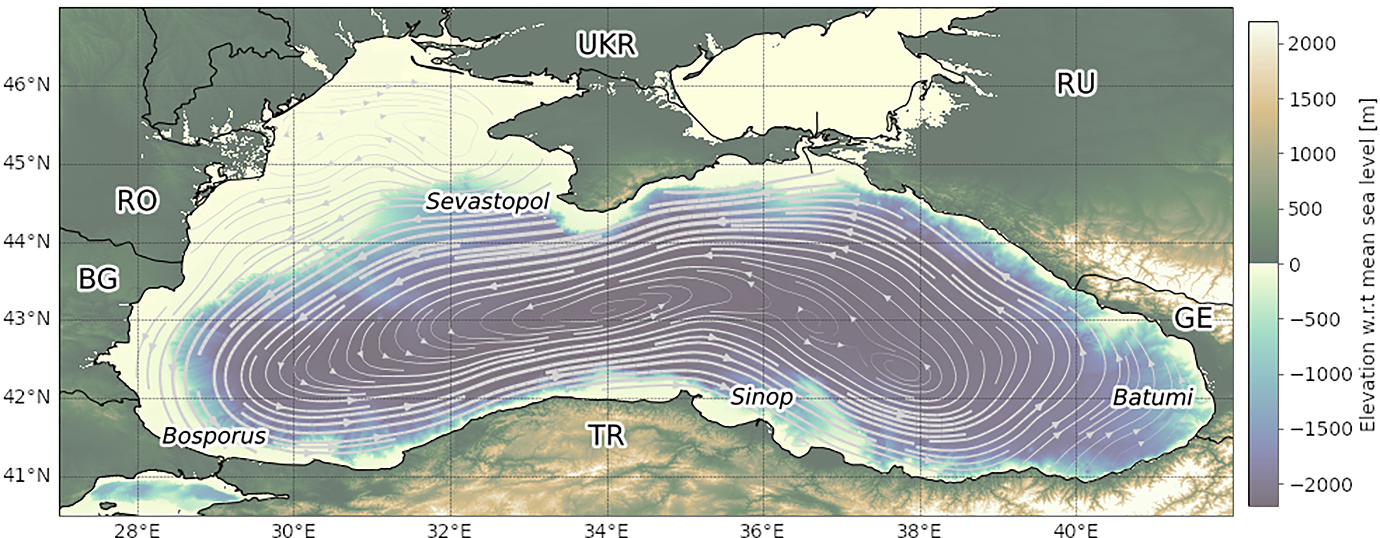
Figure 1 Elevation and bathymetry of the Black Sea region. Average circulation is obtained from (Jousset et al., 2021) and depicts the large scale cyclonic Rim current. Regional labels used in the manuscript are given in italic. Large labels are for riparian countries: UKR, Ukraine; RU, Russian Federation; GE, Georgia; TR, Turkey; BG, Bulgaria; RO, Romania.
Mesoscale activity has been studied extensively in the Black Sea, although mostly for surface manifestations. While the first qualitative studies were based on the discussion of selected scenes, synoptic data sets issued by remote sensing and automatic detection algorithms provided a statistical description of eddy properties and their dominant trajectories and revealed associated imprints on oceanic properties. Such insights helped to understand the role that mesoscale structures play in maintaining the mean state of the Black Sea environment and how they contributed to its interannual variations.
The earliest descriptions of mesoscale activity in the Black Sea relied on the combined use of dynamic heights computed from hydrographic surveys and early altimeter data (i.e., Topex-Poseidon, ERS I & II) (Sokolova et al., 2001; Ginzburg et al., 2002). While limited by data availability in terms of generalization, these studies established the adequacy of altimeter data for model assimilation purposes and already investigated the vertical dimension of mesoscale structures for specific scenes, ie. presenting evidence for the role of eddies in diapycnal exchanges and ventilation of the anoxic Black Sea interior (Sokolova et al., 2001). These early works also highlighted the high interannual variability (seasonal and interannual) in the Black Sea coastal mesoscale activity, the importance of coastal anticyclonic eddies detaching away from the coast, and evidenced associated anomalies in satellite images of surface chlorophyll-a concentration (Ginzburg et al., 2002).
A major step forward in the description of the Black Sea mesoscale circulation resulted from the assimilation of altimetry products into circulation models, thereby providing a dynamically consistent description. The synoptic nature of this approach allowed the authors to identify hot-spot areas in terms of mesoscale activity (Korotaev et al., 2001; Korotaev, 2003) and to evidence the lead factors behind the variability of Black Sea circulation patterns (Grayek et al., 2010).
Later, the first observation-based eddy census in the Black Sea was achieved by applying the ‘winding angle’ method (Kubryakov and Stanichny, 2015b,a) on maps of geostrophic current anomalies (regional merged AVISO products at a resolution of 1/8°). The principle of this method is to compute the advection of Lagrangian particles using static current fields (for each time frame) during a fixed period and to identify the particles achieving a total rotation of 360° (i.e., the winding angle). This process identifies grid cells that are located on closed streamlines and can then be labeled as edges of individual eddies. Kubryakov and Stanichny (2015b) acknowledged that the limited quality of geostrophic current products in coastal areas limited the identification of coastal eddies. To cope with this issue, the authors adopted a specific procedure and accepted that a winding angle of 270° implies a closed streamline in coastal areas. Using AVISO products for the period 1992-2011, the authors identified 847 individual eddies of both cyclonicity with a lifetime of more than four weeks and detailed the spatial and temporal variability in their properties (radius, orbital velocity,…). In particular, the authors highlighted four dominant trajectories for Black Sea eddies: 1) Eddies formed west of the Crimean peninsula (Sevastopol area, Figure 1), evolving along the continental slope to the southwest, and dissipating to the north of the Bosporus; 2) Eddies formed in the Batumi region and remaining quasi-stationary; 3) Eddies formed in the Batumi region and transformed into open sea eddies, moving northwest; 4) Eddies formed in the northeast and moving along towards the southern coast of Crimea. Noteworthy, no near-shore eddies trajectories were depicted near the Sinop region, whereas model-complemented analyses highlight quasi-permanent eddy activity in this area (Korotaev, 2003).
More recently, the optical flow inversion approach was proposed as an alternative to the altimetry-based methods for the retrieval of mesoscale surface currents (Kubryakov et al., 2018a). This method exploits satellite imagery (e.g. infrared for sea surface temperature, visible for ocean color products) to infer surface currents using a variational approach. The process consists of identifying the current field that best reproduces the advection observed between consecutive frames. It is thus based on the assumption that horizontal advection is the lead mechanism behind the changes in the distribution of a given tracer between two consecutive images. This approach, that has been compared with SLA-based approaches for selected scenes (Kubryakov et al., 2018a), has promising advantages. In particular, it offers the possibility to exploit far finer spatial and temporal resolution products (e.g., Landsat-8, Sentinel 2) and hence to characterize meso- to sub-mesoscale phenomena in more detail. The main drawback is that optical products are typically affected by cloud cover, hence do not offer the possibility of a long-term, synoptic and systematic eddy tracking procedure. Also, surface current estimates are dependent on the presence of gradients in the surface tracer, which limits, for instance, SST-based analyses in summer.
To date, the characterization of Black Sea coastal eddies thus remains a technical challenge which, in particular, limits our capacity to characterize their contribution in the Black Sea biogeochemical cycles. Indeed, novel high-frequency observations obtained by tethered (Ostrovskii and Zatsepin, 2011; Ostrovskii et al., 2018) and free-floating profilers (Stanev et al., 2013; Akpinar et al., 2017) revealed that mesoscale eddies and their interaction with the shelf-slope may substantially influence the biogeochemical balance of the Black Sea by inducing diapycnal mixing events. As vertical oxygen transport is limited in the Black Sea by a sharp pycnocline, diapycnal mixing in the basin periphery may act as a net flux of oxygen to intermediate layers, thereby enabling horizontal diffusion (i.e., along isopycnals) towards the basin interior (Ostrovskii and Zatsepin, 2016). In addition, nearshore eddies are important drivers of the horizontal exchanges between the land-influenced peripheral regions, rich in nutrient and organic matter, towards the central open sea (Zatsepin, 2003; Shapiro et al., 2010; Zhou et al., 2014).
1.3 Perspectives and Objectives
An enhanced description of mesoscale dynamics in the coastal Black Sea could thus alleviate a number of gaps in our understanding of the concerning Black Sea oxygen dynamics, in particular:
● To quantify cross-shelf exchanges induced by coastal eddies detaching from the coast and by structures emerging from the meanders of the Rim current. Those exchanges should be characterized at different pycnal levels.
● To document diapycnal mixing processes induced by the interaction of coastal eddies with the coastline/shelf break.
● To characterize the imprint of eddies on the vertical distribution of biogeochemical tracers and processes. This is in terms of advective and diffusive transport, and in terms of the biogeochemical catalytic mechanisms that may result from perturbing the vertical distribution of active biogeochemical tracers.
More specifically, in this study, we apply an eddy identification and tracking algorithm to compare three sets of remote sensing altimetry products and one issued from a model simulation. To highlight remaining gaps in altimetric products and their potential implications on cross-shelf exchanges estimates, we compare the resulting eddy censuses in terms of property distributions and dominant pathways as a function of cyclonicity, in particular along the shelf breaks. We then use Argo profiles to characterize the mean subsurface signature impressed by cyclonic and anticyclonic eddies on the mean salinity and oxygen structure. Finally, the adequacy of different altimetric products to characterize mesoscale activity in the Black Sea is discussed based on the consistency and error estimated for these composite reconstructions.
2 Material and Methods
Four different sea surface elevation data sets are used to identify eddies in the Black Sea. We describe here these data sets and present the methods used to identify eddies and their trajectories and to describe associated morphological and subsurface characteristics.
2.1 Sets of Altimetry Products
Three altimetric data sets are issued from remote sensing. A fourth similar data set, obtained from a non-assimilating hydrodynamic model, is used for comparison. All products are considered for a common period extending from the 1st of January, 2011, to the 31st of December, 2019, which is set by the limits of availability for datasets dependencies intervening in the processing of the EO4SIBS-ADT product (Cryosat-2 L3 5Hz data).
2.1.1 CMEMS-SLA
The reference altimetry data set consists of the Copernicus Marine Service (CMEMS) standard product1, whose extensive description can be found in CMEMS documentation (Taburet and Pujol, 2021). CMEMS-SLA is processed by the DUACS multi-mission altimeter data processing system and corresponds to the DUACS DT2018 version also described in Taburet et al. (2019). It includes, for the period considered, data from all altimeter missions: Jason-1, Jason-2, Jason-3, Envisat, Sentinel-3A, Sentinel-3B, Haiyang-2A, Saral/AltiKa, Cryosat-2. To produce gridded maps of Sea Level Anomalies (SLA) in delayed time, the system uses the along-track altimeter missions products2 and involves an optimal interpolation (OI) procedure. Geostrophic currents are then derived from SLA. We stress that no mean dynamic topography (MDT) is used in this processing. Instead, gridded altimeter satellite SLA is computed with respect to a twenty-year average of the observed sea surface height. This approach is similar to the long-term average mean sea level used as an MDT proxy in the first Black Sea altimetric studies (Sokolova et al., 2001; Korotaev, 2003), although that one was identified from hydrographic climatologies.
2.1.2 CMEMS-ADT
A first Black Sea MDT, consistent with the framework of the AVISO products, was then compiled using along-track sea level anomalies, surface drifters, and hydrographic survey (Kubryakov and Stanichny, 2011), and used for subsequent works (e.g. Kubryakov and Stanichny, 2015b; Kubryakov et al., 2016; Stanichny et al., 2016; Kubryakov et al., 2018a; Kubryakov et al., 2018b; Zatsepin et al., 2019). Later, Menna and Poulain (2014) proposed a revised MDT, expressed in terms of geostrophic currents and based on a larger number of drifter data. Yet, until recently, there was no official MDT product available in the AVISO/CMEMS reference data sets for the Black sea region, and only sea level anomalies and corresponding geostrophic velocities were available from altimetry products. While CMEMS-SLA has been the reference product for many years, the last update (May 2021) of the CMEMS catalog now provides an MDT for the Black Sea (Jousset et al., 2021), which enables the use of absolute dynamic topography (ADT), which should generally be preferred to SLA for eddy detection in regions where mean circulation and mesoscale features are close in terms of spatial scale and intensity, and where the MDT may embed quasi-permanent mesoscale patterns (Pegliasco et al., 2021). CMEMS CMEMS-ADT is thus identical to CMEMS-SLA in terms of spatial resolution, along-track data preprocessing, and gridding methodology, but ADT is now used instead of SLA for the identification of eddies.
2.1.3 EO4SIBS-ADT
This new product was developed in the frame of the ESA project EO4SIBS3. Enhancements with respect to CMEMS products were brought to both L3 (along-track) and L4 (gridded) processing steps.
The major difference in the L3 processing consists of processing full rate (20Hz) altimeter measurements rather than conventional low resolution (1Hz) measurements to better access small scale signals for Cryosat-2 (C2) and Sentinel-3A (S3A) missions. This was made possible by recent advances in altimeter technology and processing. The SAR technology available on C2 and Sentinel-3 missions, as well as innovative re-tracking methodologies (e.g. Moreau et al., 2021), contribute to significantly reduce the measurement errors at short wavelengths. The procedure for the along-track processing steps includes valid data selection, long-wave error correction (to remove local discrepancies between neighboring tracks), short wave noise reduction, and subsequent resampling (to reach a final along-track data selection at 5Hz).
Enhancements brought to the L4 processing steps (gridded products) involve the consideration of a bathymetric constraint in the optimal interpolation procedure [as successfully tested in Escudier et al. (2013)], the consideration of eddy propagation velocities (deduced from the CMEMS BS-MFC-BIO model described below) in the correlation scale definition, and the refinement of the gridded product resolution (1/16° compared to 1/8° for CMEMS-ADT). The bathymetry used in this process is the same as used in the frame of the CMEMS BS-MFC-BIO modeling efforts (Grégoire et al., 2020), which provided the model simulation described below. For its consideration in the optimal interpolation procedure, this bathymetry has been filtered using a low-pass Lanczos filter at a 50 km cut-off wavelength. This wavelength was chosen to avoid creating spurious eddies in the areas by extrapolating very small structures below the resolution capability of the OI. The altimetry products and their specifications may be found on the EO4SIBS project’s website.
The main differences between CMEMS and EO4SIBS L4 products are observed in Eddy Kinetic Energy (EKE), which highlights the variability of surface currents around their mean value and therefore relates to eddy activity. The EKE differences (Figure 2) underscore both the coastal areas and the continental slope with higher EKE observed in the EO4SIBS product. The main part of this additional energy is explained by the bathymetric constraint used in EO4SIBS processing, which is expected to enhance EKE near bathymetric gradients as illustrated by Escudier et al. (2013) for the Mediterranean Sea. Nearshore, the improved data availability, and thus the signal observability offered with 5Hz along-track product (Sentinel-3A and Cryosat-2), also contributes to this result. For more information on the EO4SIBS-ADT dataset, please refer to the EO4SIBS website.
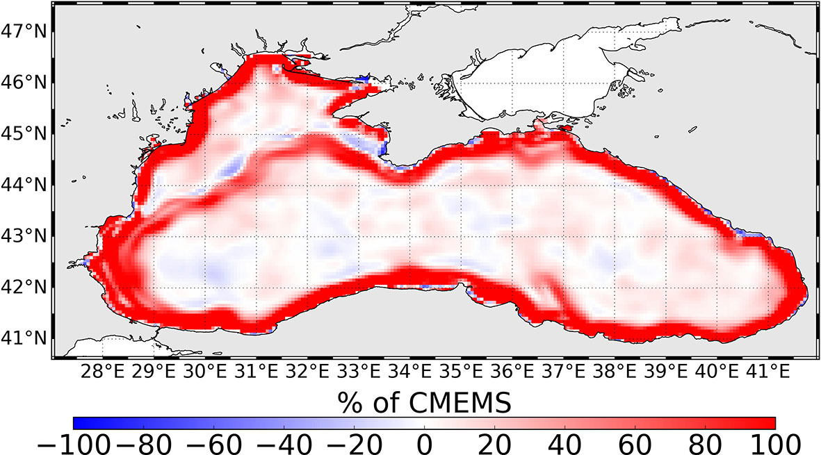
Figure 2 Relative differences in mean eddy kinetic energy obtained from EO4SIBS-ADT and CMEMS-ADT products.
2.1.4 Model
To complement the comparison of eddy properties obtained from the different remote sensing products, we consider the sea surface elevation dynamics provided by the CMEMS BS-MFC-BIO simulations. This setup involves the hydrodynamic model NEMO 3.6 at a spatial resolution of 3km with 31 vertical z-levels Grégoire et al. (2022), which can be tagged as “eddy-resolving” according to the criteria given by Staneva et al. (2001). Per nature, model-derived sea surface elevation consists of ADT values.
Model products provide an interesting basis for comparison given their underlying theoretical framework, and it is certainly comforting when the descriptions of eddy properties obtained from the model and remote sensing products converge. Yet, both approaches suffer from their own limitations. While relevant for discussion, we do not consider model results as a strict reference to characterize the accuracy of the remote-sensing eddy censuses or to rank the skill of altimetric data sets in accurately describing the real mesoscale circulation field. Previous studies have indeed shown a strong sensitivity of the resolved mesoscale features towards internal parameterization (Zhou et al., 2014). This is one of the reasons why we investigated on the use of Argo profiles as an independent data set potentially relevant to characterize the accuracy of altimetric products.
It arises from the above description that the altimetric products differ in many aspects (Table 1). Resulting differences in eddy properties may thus originate from 1) the use of ADT instead of SLA, 2) enhancement brought to the along-track sampling and processing 3) enhancement brought to the production of gridded products, 4) a refined resolution of the interpolated gridded products. It is beyond our scope to detail the respective impacts of these different processing steps on eddy properties. Rather, we compare these products as successive “state-of-the-art” and describe the successive levels of detail obtained in the characterization of the Black Sea eddy activity.

Table 1 Main processing differences between the four altimetric data sets.
2.2 Eddy Identification
Eddy identification and tracking is carried out with the open-access py – eddy – tracker code4 (Mason et al., 2014). After preliminary tests, we disregarded any pre-filtering of the daily Black Sea altimetric fields. This procedure is generally advised in the open ocean, but may not be as relevant for regional seas of limited extension.
The py – eddy – tracker code searches for closed SLA contours at intervals of 2mm, downwards and upwards for cyclones and anticyclones, respectively. At each SLA interval, closed contours are sequentially considered for selection as a potential eddy, which requires to:
1. Pass a shape test with error ≤ 70%, where the error is defined as the ratio between the areal sum of deviations of the closed contour from its fitted circle, and the area of that circle.
2. Contain a pixel count, l, satisfying lmin ≤ l ≤ lmax where lmin = 5 and lmax=2000.
3. Contain only pixels with SLA values above (below) the current SLA interval value for anticyclones (cyclones).
4. Contain no more than one local SLA maximum (minimum) for anticyclones (cyclones).
The contour meeting those requirements is defined as the effective contour of a newly identified eddy. An internal contour is then identified as the inner contour along which the circum-averaged orbital velocity is maximal.
As we compare products with distinct spatial resolution, we should stress that the minimal extent of the eddies is given in pixel count, which thus corresponds to smaller areas for high-resolution products5. In addition, the forbidding of multiple internal extrema may penalize large eddies in the high-resolution products. It is thus naturally expected that high-resolution products may lead to more small eddies and less large eddies.
Once an eddy is identified, several parameters are estimated: the longitude and latitude of its center and effective contour; its effective radius (R), ie. the radius of a circle with equal area; its amplitude (A), ie. the difference in elevation between the eddy center and effective contour and its orbital velocity (V), ie. the rotational velocity circum-averaged along the eddy internal contour. The data structure adopted within py – eddy – tracker and its post-processing tools associates these properties with instant eddy locations, which largely ease the generation of summary figures such as provided below. We note that there exists a vast range of eddy tracking methodologies (and fast-expanding) that have been proposed to overcome some known limitations (Amores et al., 2018) of the traditional gridded-altimetry elevation contours approach adopted here. Comparing these algorithms falls beyond our scope. Also, we opted for the above methodology for its large established usage and practicality.
2.3 Eddy Tracking
To produce individual eddy tracks, ie. a series of instant eddy contours considered to represent different time instances of the same eddy, the algorithm considers the consecutive daily files of identified eddies. The tracking is thus carried out in a separate step from the identification, treating cyclones and anticyclones separately. Following Pegliasco et al. (2015), two eddies P0 and P1 from subsequent daily images are considered to be successive pictures of the same eddy if c > 0.2, where c is an overlap score:
Because altimetry products are imperfect, a long-lived eddy may at any time be inadvertently interrupted during the tracking process. This will result in shorter track duration statistics than might be expected. To alleviate this known issue, the eddy tracker allows for the optional use of virtual eddies that attempt an online filling in of these gaps. We activate this option with a conservative setting of 2, implying that the code will place a maximum of two virtual eddies along the expected path of the eddy. If there is then a continuation, i.e., a previously identified eddy is within range of the virtual eddy, the code will continue iterating until the eddy dies. If there is no continuation, the code will end the iteration.
Finally, only eddies with a lifetime larger than two weeks were retained for further analysis. Methods and codes used to identify and collect eddy properties are largely documented in the py – eddy – tracker documentation pages6.
2.4 Composite Analyses of Argo Profiles
To characterize the subsurface field perturbations associated with eddies, in-situ profiles of salinity and oxygen recorded by Argo floats are re-allocated in a common frame of eddy-centric coordinates. To do so, we exploit the coordinates of eddy centers and contours obtained from the identification and tracking procedure. This implies that the characterization of subsurface perturbations is directly dependent on the accuracy of the altimetric product.
Temperature was not considered here, as subsurface temperature perturbations induced by eddies are largely season-dependent, due to the characteristics of the Black Sea temperature profile seasonal variations, cf. Cold Intermediate Layer dynamics, (Ivanov et al., 1997; Piotukh et al., 2011; Capet et al., 2014). Considering temperature would thus require further seasonal subsampling, which was not considered relevant for the present study.
A complete record of Argo and BGC-Argo profiles active in the Black Sea between 2011 and 2019 was obtained from the Coriolis center in the form of synthetic profiles (Bittig et al., 2021). We only retained floats with an active lifetime above 180 days within the considered period, which resulted in 29 profilers equipped with salinity sensors, and 12 with oxygen sensors. Of those, respectively 27 and 12 floats were spotted at least once within an eddy contour. With an average lifetime of about 1000 days (maximum 2290 days), these floats provided, in total, 6143 salinity and 2350 oxygen profiles, of which between a tenth and a fifth could be assigned within eddy contours (Table 3). Their temporal sampling frequency varies between 1, 5 and 10 days. The spatial density and coverage of these profiles are illustrated in Figure 3.
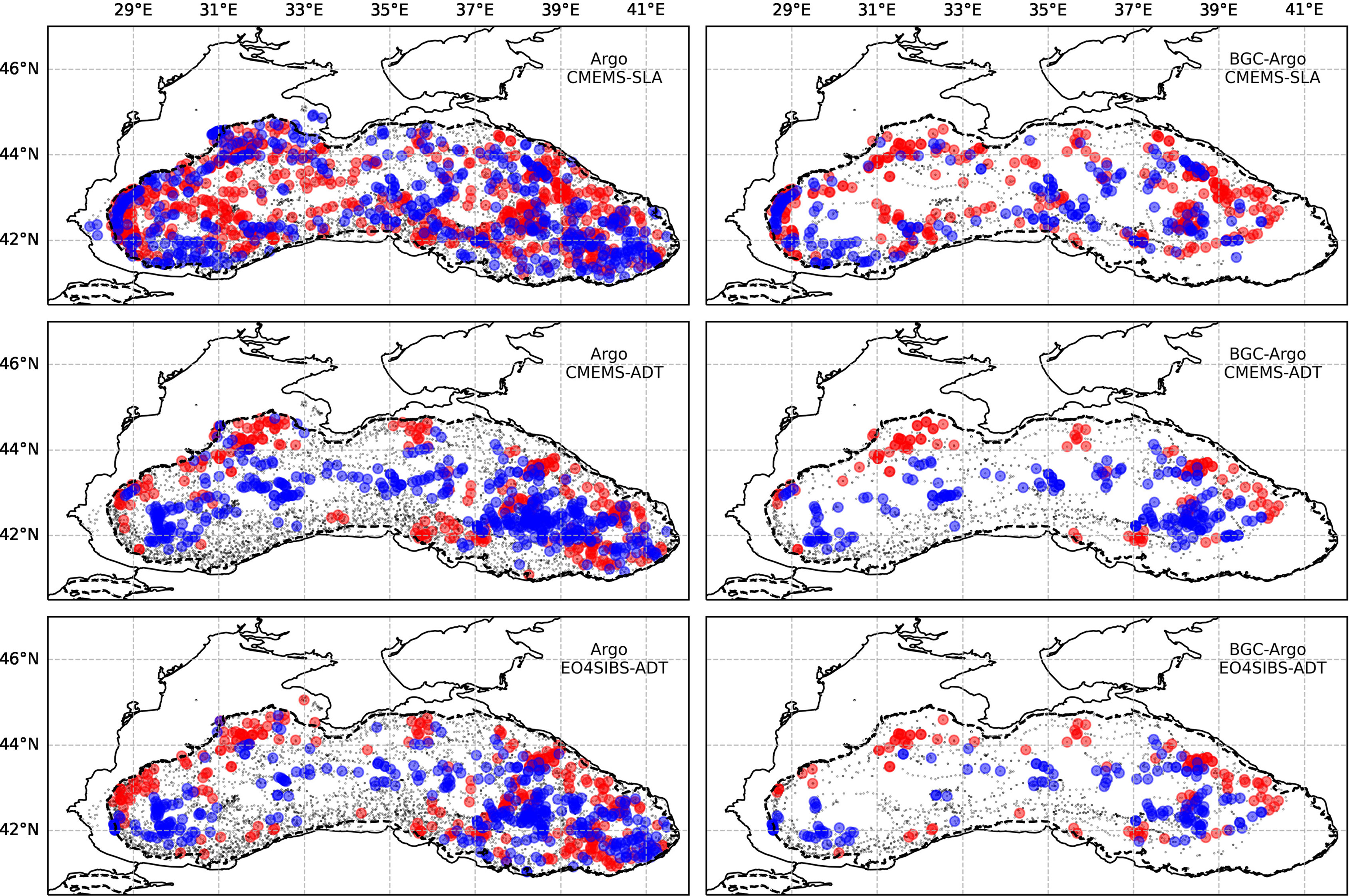
Figure 3 Location of the (left) Argo and (right) BGC-Argo profiles. Match-ups obtained with different altimetric product are highlighted for (blue) cyclones and (red) anticyclones. The dotted line indicates the 200m isobathymetric contour.
Subsurface perturbations refer to anomalies with respect to the mean vertical structure of the considered variables (salinity or oxygen). Instead of the instant values recorded by Argo profilers, we thus consider the anomalies of individual profiles with respect to a temporally smoothed signal, obtained specifically for each float. The smoothing was obtained by applying a rolling median along the time dimension, considering a rectangular window of 6 months, operated for each 5m depth layer between 5 and 500m independently (an illustrated example is provided in Figure S1). The purpose of this filtering procedure was to identify eddy perturbations as anomalies with respect to the regional and seasonal typical profile. We favored this option against using long-term climatological products due to the important interannual variability that affected the Black Sea during the recent decades. The 6-months time window was adopted after iterative inspections and considering the typical eddies lifetime (Table 2), and contiguous period spent by Argo floats within identified eddies (maximum 40 to 80 days, depending on the altimetry product). We believe similar assessments should be conducted before transposing the methodology to other areas.
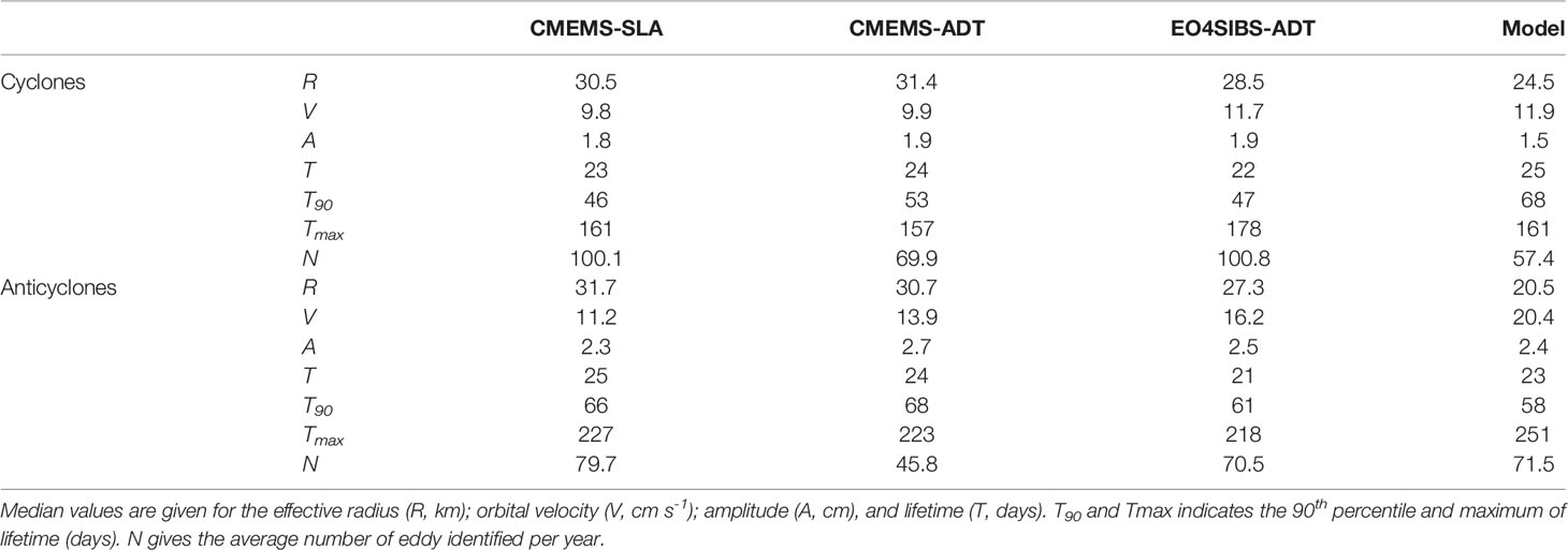
Table 2 Eddy properties obtained from the different altimetric products and the model equivalent.

Table 3 Number of match-ups obtained for the three remote sensing altimetric data sets.
All match-up cases were then identified, i.e., when an Argo profile is located within the effective contour of an identified eddy. The corresponding anomaly profiles were extracted from the BGC-Argo time-series and relocated in an eddy-centric coordinate system, for cyclones and anticyclones, respectively. This coordinate system only considers the distance between the float and the eddy center at the time of match-up, which is normalized by the eddy radius at the time of match-up.
Subsurface anomalies in the oxygen and salinity vertical structure were then characterized by averaging all profiles within bins of normalized distance from the center, using bin widths of 1/6 eddy radius to ensure a decent number of profiles within each bin. Finally, the standard error on these mean values were obtained using , where σ is the standard deviation within a bin, and N the number of observations (see discussion Sect. 4.4). A two-tailed t-student test is used to assess the p-value of having a mean anomaly that is significantly different from zero, thus using the number of profiles available for each bin.
3 Results
In this section, we describe the differences in eddy properties as obtained from the four data sets. We first focus on surface eddy morphological and trajectory properties, comparing results obtained from the altimetry and model products, and then address the subsurface composite anomalies obtained from Argo oxygen and salinity profiles.
3.1 Properties of Individual Eddies
The differences that arise in eddies properties and census when applying the same tracking methodology on the different altimetry products are more pronounced for anticyclonic eddies, in particular in terms of effective radius and speed average (Table 2).
At equal resolution, the consideration of ADT (instead of SLA) substantially reduces the number of identified eddies (see CMEMS-SLA and CMEMS-ADT in Table 2). The impact on property distributions is minor for cyclones (Figure 4), and only involves a slight shift towards higher velocities for anticyclones.
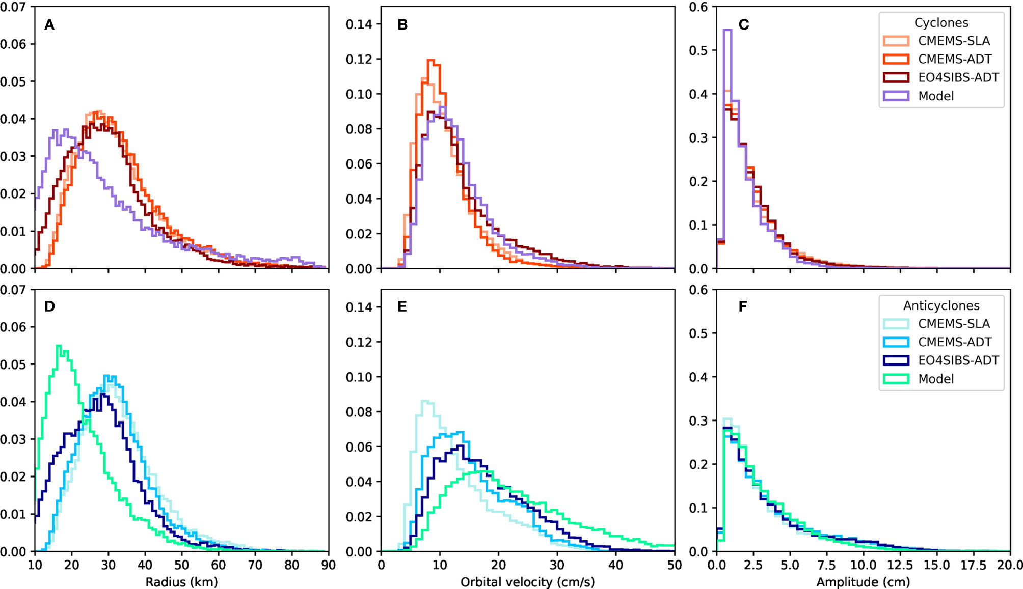
Figure 4 Distribution of eddy properties as obtained from the different data sets for cyclones (A–C) and anticyclones (D–F): effective radius (A, D), orbital velocity (B, E) and amplitude (C, F).
The enhanced EO4SIBS processing (see. 2.1) substantially increases the number of identified anticyclones (+54%) and cyclones (+44%). It also increases the density of small (< 20km) cyclones and anticyclones and reduces that of medium and large eddies (>40km). Notably, the shifts induced in eddy property distributions when considering EO4SIBS-ADT instead of CMEMS-ADT systematically bring them closer to the model descriptions. While a close match is observed between EO4SIBS-ADT and model velocity distributions for cyclones, anticyclones are described in the model product with even faster orbital velocities. This difference in the evolution of the cyclones and anticyclones R and V distributions along successive data sets will later be discussed considering the coastal predominance of anticyclones. Distributions of amplitude remain relatively unchanged, with the notable exception of a reduced number of high amplitude cyclones in the case of the model products.
It should be stressed that all data sets provide lifetimes shorter than 10 weeks for the vast majority of eddies (90%). The median lifetimes lie around 24 days both for cyclones and anticyclones and do not vary substantially from one data set to the other. Yet, long-lived anticyclones are more numerous than their cyclonic counter-part (T90 is larger by 33% for anticyclones than it is for cyclones, on average for the three altimetric products, ie. 65 days and 49 days respectively), while the longest identified eddy tracks last for about 220 days for anticyclones and 165 days for cyclones.
Considering the evolution of eddy properties along their normalized lifetime (Figure 5) leads to this general statement: the consideration of ADT products provides a better distinction between the properties of cyclones and anticyclones, a difference that grows as the eddies develop. Model outputs, which unlike the altimetric products can be considered of spatially homogeneous quality, provide an even stronger differentiation between cyclones and anticyclones properties. Noteworthy, the model-based description of the evolution of anticyclones properties along lifetime departs from the time-reversal symmetry generally observed for open sea eddies (Samelson et al., 2014), which may originate from a difference in the driving factors affecting their evolution through time, i.e., interaction with other eddies for open-ocean eddies, and interaction with the shelf-slope for the coastal anticyclones).
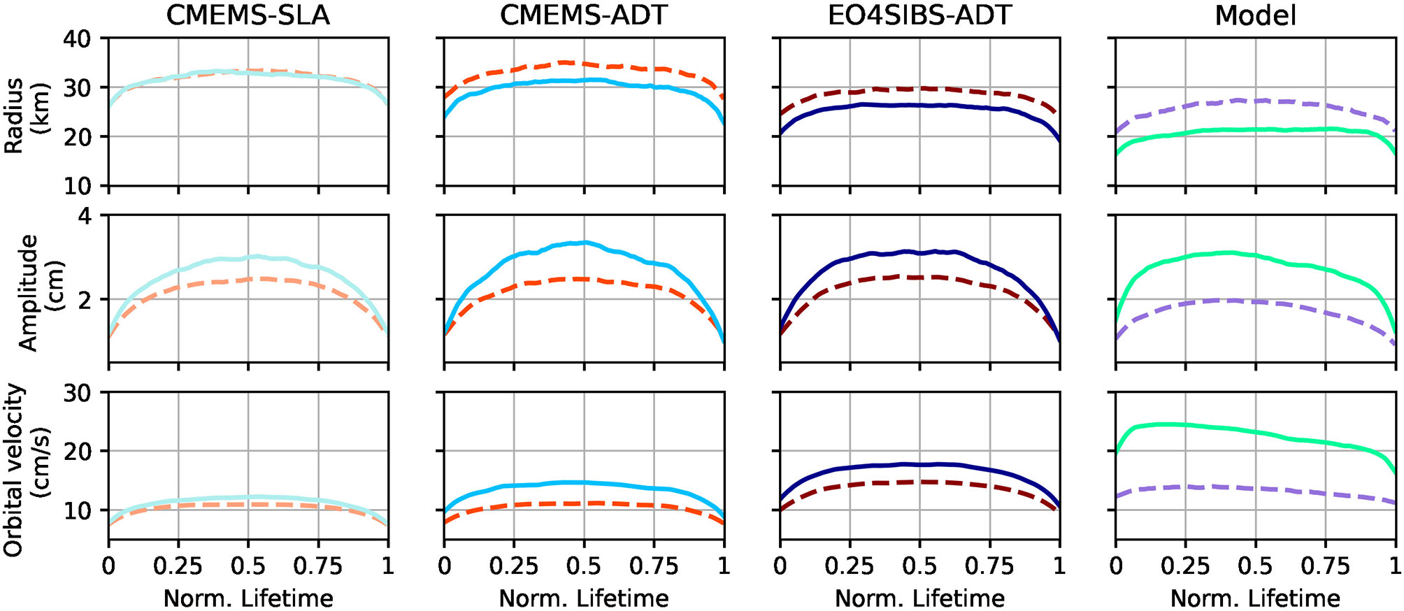
Figure 5 Evolution of the average properties of (dotted lines) cyclonic and (plain lines) anticyclonic eddies along their normalized lifetime.
3.2 Spatial Distributions and Trajectories
While CMEMS-SLA barely distinguish regions of dominant cyclonicity (Figure 6A), the use of ADT reveals the well documented anticyclonic and cyclonic regions of the Black Sea (Figure 6B), in the peripheral and central region of the basin, respectively. EO4SIBS-ADT (Figure 6C) provides slightly more continuity in the anticyclonic regions located along the northwestern, southern, and northeastern shelves which is in agreement with the dynamic considerations embedded in the production of the model outputs (Figure 6D). Besides, EO4SIBS-ADT, which benefits from enhanced prepossessing targeting the coastal areas, provides a better-defined distinction between coastal and central eddies formation area, in particular for anticyclones along the southern and northeastern shelves (Figure 7).
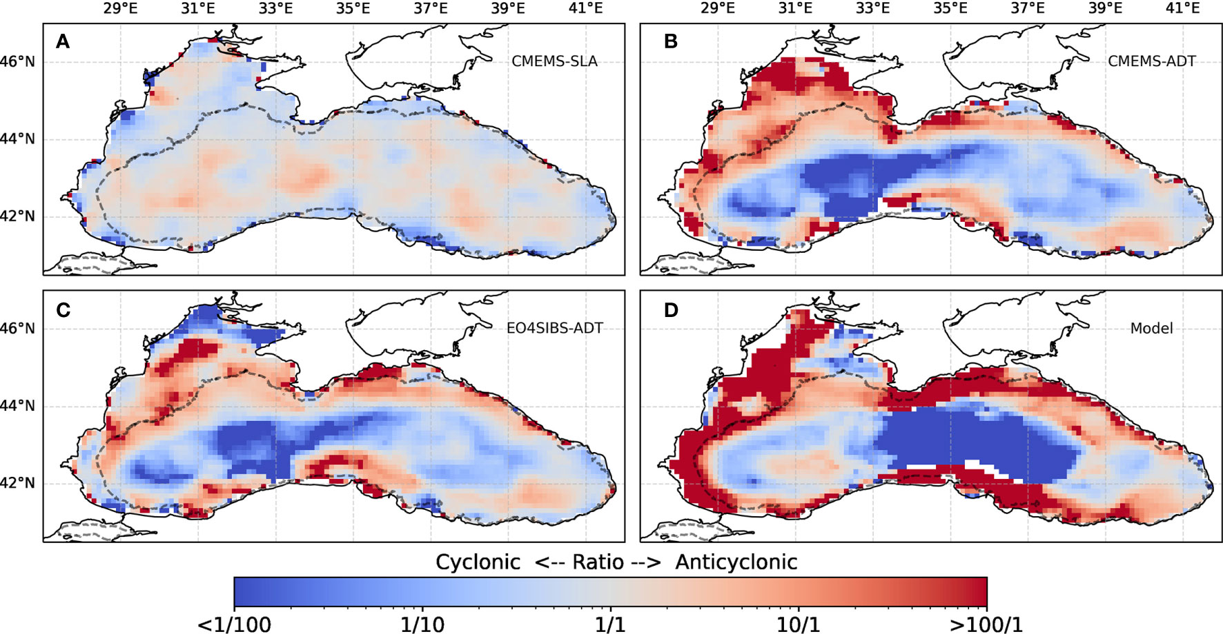
Figure 6 Ratio between the number of days passed within cyclones or anticyclones, as obtained from the different data sets : (A) CMEMS-SLA, (B) CMEMS-ADT, (C) EO4SIBS-ADT, (D) Model. The dotted line indicates the 200 m isobathymetric contour.
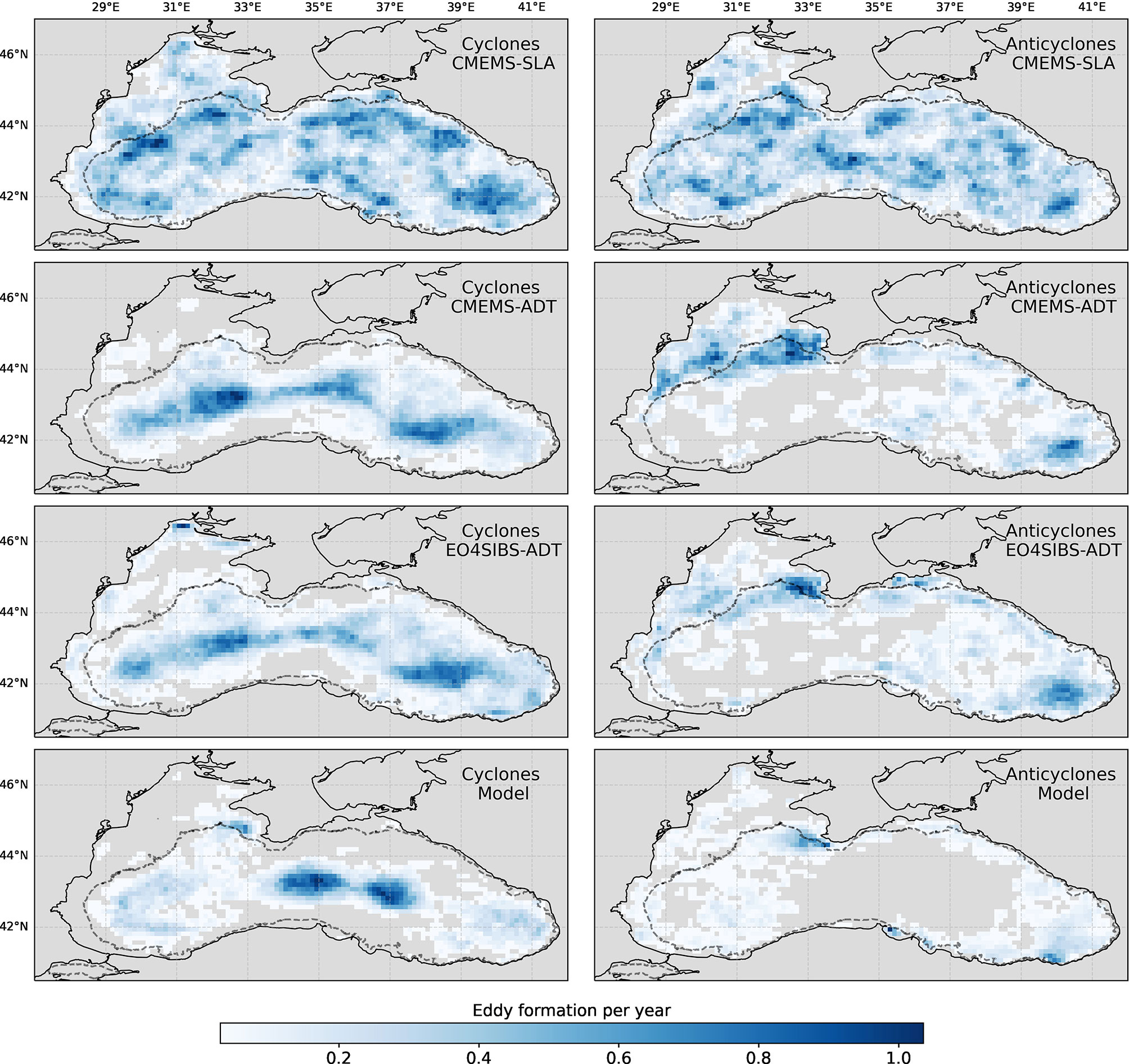
Figure 7 Annual frequencies of eddies formation events, including both cyclones and anticyclones, as obtained from the different data sets. The dotted line indicates the 200m isobathymetric contour.
This clearer distinction also prevails between cyclones and anticyclones pathways (Figure 8). EO4SIBS-ADT more clearly depicts the tendency for anticyclones to remain along the outer side of the rim current, along the shelf break, while cyclones issued from the same areas show a tendency to drift towards the basin center. This tendency appears quite clearly in the model results for eddies generated at the western and eastern shelf breaks. Finally, the case of the Sinop region (42°N, 36°E) is particularly illustrative. The two host-spot anticyclonic formation areas, that are strongly pronounced in the model results (Figure 7, 8), can be discerned from EO4SIBS-ADT, but not from CMEMS-ADT.
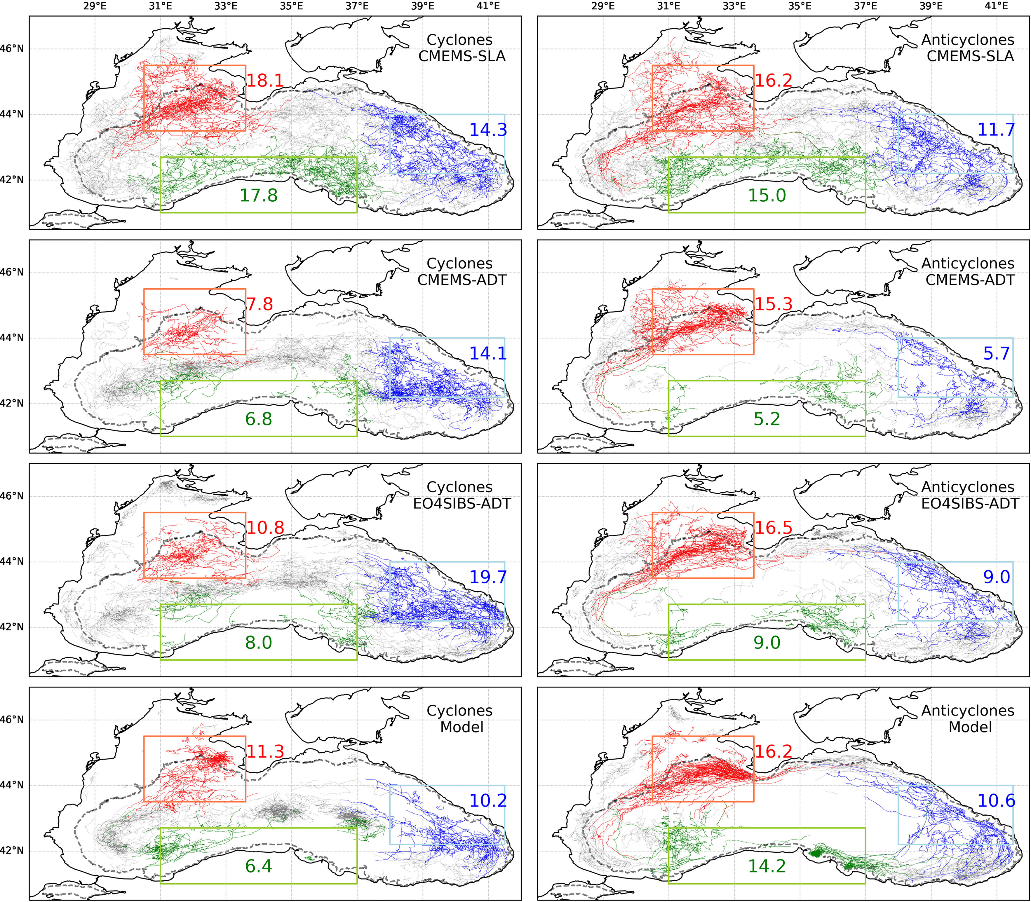
Figure 8 Dominant cyclone (left) and anticyclone (right) pathways for three shelf regions of the Black Sea, as obtained from the different data sets. All the identified eddy tracks are displayed in grey. Tracks crossing the colored boxes are then highlighted in the same color as the box. The colored numbers provide the yearly count of such tracks for each of the three regions. The dotted line indicates the 200m isobathymetric contour.
3.3 Subsurface Anomalies
The census and morphological properties of eddies thus depend on the input altimetry data set, as do the normalized eddy-centric coordinates assigned to Argo profiles. Also, the number of profiles that can be exploited to characterize the subsurface signature of eddies vary between altimetric products, as it depends on the number of identified eddies, their location and radius.
The number of match-ups strongly decreases when considering CMEMS-ADT instead of CMEMS-SLA, in particular for anticyclones (Table 3, -39%), in a ratio that is similar to the ratio obtained between eddy counts (-36%). While the new product EO4SIBS-ADT provides a larger eddy count than CMEMS-ADT (+48%), the number of match-ups further decreases (-18% and -7% for BGC-Argo and Argo, respectively), which is likely attributed to the facts that 1) effective radius distribution is shifted towards smaller values (Figure 4) and 2) that additional eddies are mostly located in near-shore regions (Figure 8) where Argo profiles are generally scarcer. From geometric considerations, it is expected that the number of match-ups decreases more rapidly for smaller radial distances to eddy centers (Figure 9). Also, because eddies are not systematically circular, it happens that an Argo profile spotted inside an eddy effective contour has a distance to the center that is larger than the computed effective radius.
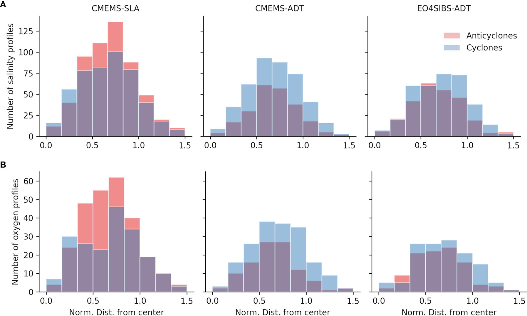
Figure 9 Number of exploitable Argo profiles for different relative distances to an eddy center (ie. the distance normalized by the effective eddy radius). (A) Argo, (B) BGC-Argo.
Despite a lower number of exploitable profiles, using CMEMS-ADT instead of CMEMS-SLA to identify the eddy-relative location of in-situ profiles provides a better characterization of subsurface anomalies. For salinity (Figure 10), this better characterization consists of a clearer gradient of the anomaly from the eddy center to its periphery, an increase in the magnitude of the anomaly near the center (up to -0.7 p.s.u at a core depth of 100 m for anticyclones), and expansion of the area where the mean anomaly can be considered as significantly different from zeros. Similar observations arise for oxygen (Figure 11): expansion of the significant area, clearer gradient, and increase in intensity. In particular, the composite oxygen anomaly obtained for cyclones on the basis of CMEMS-SLA products depicts larger intensity beyond the eddy’s periphery, which is in direct opposition with the radial gradient obtained with CMEMS-ADT and EO4SIBS-ADT products.
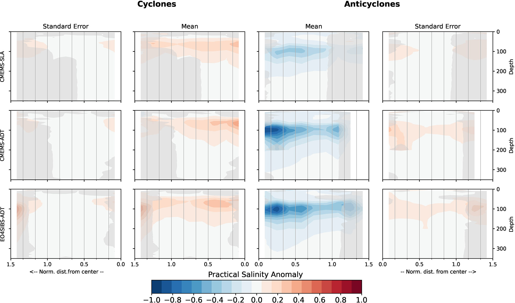
Figure 10 Characterization of subsurface salinity anomalies associated with (left panels) cyclones and (right panels) anticyclones. (Central panels) mean anomaly, (external panels) standard error on the mean. The shaded area covers regions of the eddy-centric coordinate systems where the mean anomalies cannot be considered as statistically different from zero with a confidence level of 95%.
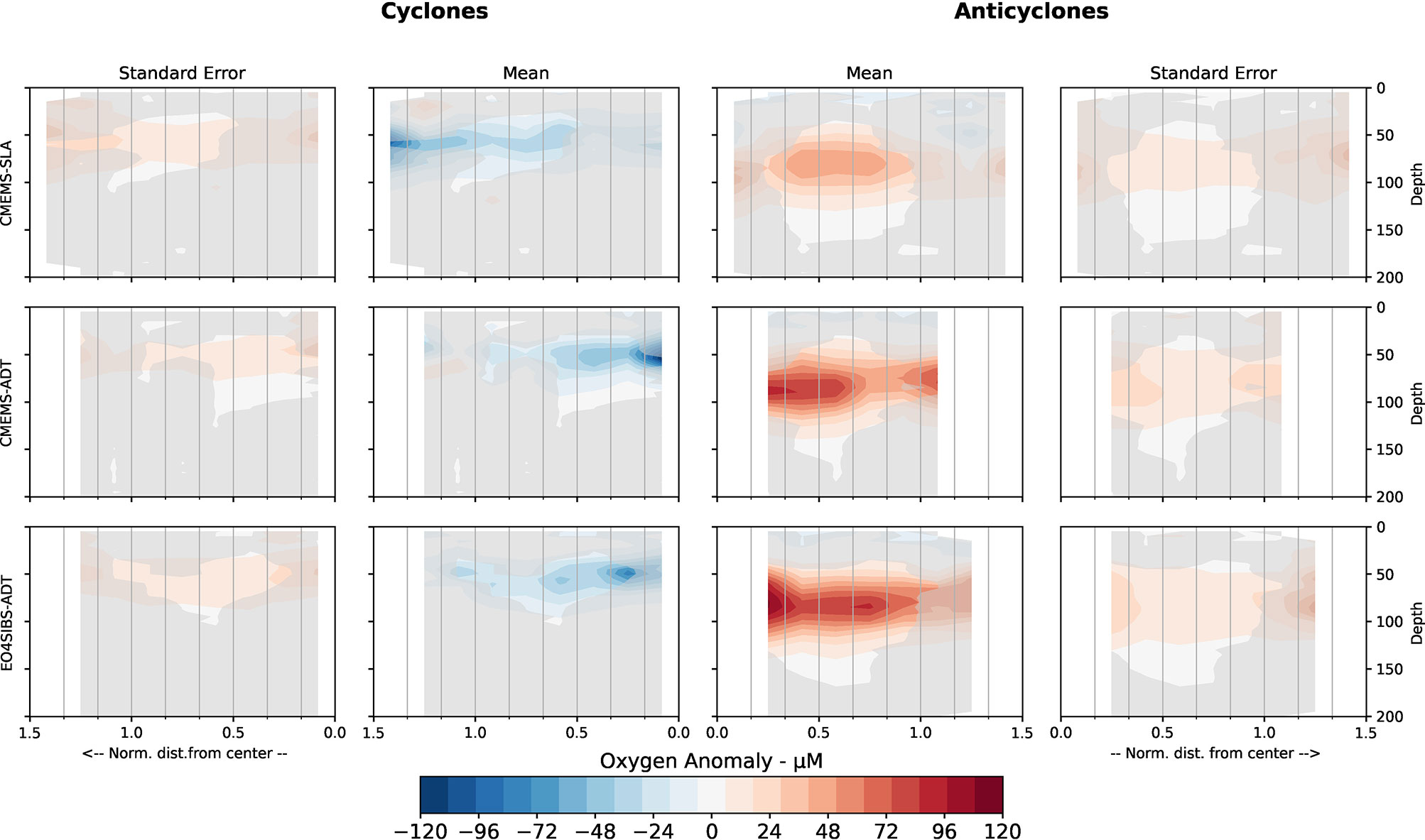
Figure 11 Same as Figure 10 for Oxygen.
The changes in depicted subsurface anomalies when evolving from CMEMS-ADT to EO4SIBS-ADT are clearer in the case of oxygen. Again, the area of significant non-zero mean anomaly is slightly expanded for anticyclones, and the gradient from center to periphery is more clearly marked. However, the lesser number of match-ups is penalizing near the center, in particular as concerns cyclones.
The subsurface eddy-induced oxygen anomalies obtained with the EO4SIBS-ADT product depict a number of interesting aspects. First, the intensity of the anomaly is large and reaches up to 100μM at a core depth of 80m for anticyclones (60μM at 50 m for cyclones). Second, a strong asymmetry arises between the cyclonic and anticyclonic cases, both in terms of intensity and depth of the anomaly. Finally, negative anomalies can be spotted near the surface, both for cyclones and anticyclones, which could not be significantly characterized based on the altimetric products CMEMS-SLA and CMEMS-ADT.
4 Discussion
4.1 Considering ADT Products Instead of SLA
The consideration of ADT products, whose effect can be assessed by comparing CMEMS-ADT and CMEMS-SLA results, induces a clearer distinction between the properties and distribution of cyclones and anticyclones. The fact that ADT products lower the number of identified eddies agrees with the conclusions of a similar comparative study conducted in the Mediterranean sea (Pegliasco et al., 2021). In our case, however, the obtained median effective radius is larger for cyclones and smaller for anticyclones, whereas ADT products systematically led to a smaller radius in the Mediterranean study. Also in agreement with this study, ADT products provide a much clearer delineation in the average cyclonicity (Figure 6), with cyclonic regions being confined to the basin center and anticyclonic dominating the peripheral regions. This is in clear agreement with the general descriptions of mesoscale activity in the Black Sea (Korotaev, 2003; Kubryakov and Stanichny, 2015a).
As concerns subsurface anomaly, the average radial structure obtained with ADT products for the oxygen and salinity subsurface anomalies, with a maximum in the eddy center, is more consistent with results obtained in other areas (e.g., Pegliasco et al., 2015; Schütte et al., 2016). In fact, the subsurface oxygen anomaly obtained from CMEMS-SLA for cyclones even depicts an opposite radial gradient with larger intensity beyond the eddy’s periphery, which makes little sense (for reasons of continuity the anomaly should decrease to zero towards the external background field) and opposes the results obtained with ADT products. Furthermore, ADT products result in larger area of the cylindrical coordinate system where the mean anomaly is significantly different from zero, even though fewer match-ups could be used to reconstruct these composite pictures. These Argo-based composite reconstructions thus demonstrate the better adequacy of ADT-based eddy censuses to reconstruct eddy signatures out of auxiliary data sets, and therefore suggest a higher accuracy of ADT-based eddy contours, in agreement with the suggestions made by (Pegliasco et al., 2021) for similar basin morphologies.
4.2 Impact of Considering High-Resolution Products
The clearest emerging property that arises from the consideration of the altimetry product EO4SIBS-ADT is a better distinction between the respective dynamics of cyclones and anticyclones. The shifts in the distributions of radius and orbital velocity are in large part associated with the refinement in the product’s spatial resolution. It is particularly interesting that this evolution of property distributions is different for cyclones and anticyclones. Similarly, while the distribution of orbital velocity obtained from EO4SIBS-ADT matches that provided by model results for cyclones, it still underestimates model orbital velocities obtained for anticyclones. In that sense, it appears that further enhancements of the altimetry products are important to resolve the asymmetry between cyclones and anticyclones properties and behavior in the Black Sea.
The difference between cyclones and anticyclones properties and distribution has been known for long as an important Black Sea characteristic (Korotaev, 2003), and can be explained by formation mechanisms (Zatsepin et al., 2019). However, the coastal segregation of anticyclonic eddies (Sect. 3.2) highlights the importance of further coastal-refined altimetry products for the Black Sea. Indeed, it makes anticyclones crucial contributors in the mediation of horizontal coastal-open exchanges and vertical (diapycnal) transport Zatsepin (2003). Thereby, the coastal refinement of EO4SIBS-ADT actualizes several questions.
A first point of interest concerns the fate of anticyclonic eddies formed along the different shelf breaks. A clear white stripe borders the coastline in the maps of anticyclonic tracks when considering CMEMS products CMEMS-SLA and CMEMS-ADT (Figure 8). EO4SIBS-ADT provides a better coverage for those areas, in particular for the southern and northeastern shelves (respectively highlighted in green and blue in Figure 8). As previously mentioned, the anticyclonic formation hot spots near Sinop and Samsun appear as a clear improvement, considering the good agreement with model outputs. However, model products indicate longer tracks for those anticyclones than those depicted from altimetric products. The same is true for eddies generated near the Bosphorus area, that travel along the Anatolian shelf in the model results but appear as interrupted in the altimetry results.
Also, spurious track interruptions are a known issue in the field of eddy tracking and can be mediated by different protocols, such as the virtual eddies embedded in py – eddy – tracker, or other approaches commonly resorted to in Black Sea mesoscale studies (Kubryakov and Stanichny, 2015b; Kubryakov et al., 2018b). However, these protocols may also artificially affect inferred eddy properties, and lifetime in particular. For the sake of illustration, (Kubryakov and Stanichny, 2015b) reports that 11% of identified anticyclones structures had a lifetime longer than 180 days, a value that is about three times larger than the T90 values reported in Table 2.
Solving this issue should be prioritized upon further enhancements of coastal altimetric data products for the Black Sea. The extent to which coastal anticyclones maintain a consistent dynamic structure while traveling along the shelf (or conversely if they rather consist of short-lived structures arising from meanders of the Rim current) has large implications regarding the estimate of their net effect in mediating material and energetic transport across the basin. For instance, to know whether eddies formed in the land-influenced Sevastopol region (44.5°N, 33°E) breaks before or after nearing the Bosporus region might be particularly important for biogeochemical considerations.
A second question of importance concerns the bifurcation of cyclonic and anticyclonic tracks issued from common formation areas. As analyzed by Kubryakov et al. (2018c) for physical properties and depicted in Sect. 3.3 for the case of oxygen, cyclones and anticyclones carry anomalies of opposite signs. A bifurcation in their advection tracks would thus result in net transport terms to be considered while exploring the processes maintaining horizontal patterns in the vertical distribution of these properties.
4.3 Oxygen Subsurface Anomalies Associated With Eddies
The asymmetry between the subsurface oxygen anomalies associated with cyclones and anticyclones (Figure 11) is of particular relevance for the study of Black Sea oxygen dynamics. The different intensity in induced oxygen anomaly indeed suggests that the positive anomalies associated with anticyclones arise from more than a mere vertical displacement of isopycnal layers. In parts, this asymmetry may arise from the shape of the underlying mean oxygen profile. A similar asymmetry is indeed visible for salinity (Figure 10), to a lesser extent, for which the introduction of additional source/sinks terms is excluded. In the case of oxygen, however, the positive anomaly associated with anticyclones is much larger in amplitude than the negative anomaly associated with cyclones. This suggests an overall efficient ventilation of the upper oxycline by eddy stirring, as demonstrated for the Peruvian OMZ (Bettencourt et al., 2015), where eddy oxygen fluxes towards the OMZ were estimated to be one order of magnitude larger than mean fluxes, and suggested for the Black Sea by Ostrovskii and Zatsepin (2016). By opposition to open ocean eddies where enhanced primary production and trapping of organic matter induces overall negative oxygen anomalies in the eddy cores (Schütte et al., 2016), it seems that eddy stirring and subsequent ventilation overweight enhanced primary production and subsequent respiration in the stratified Black Sea, thus resulting in overall positive oxygen subsurface anomalies.
We further note that subsurface eddy-induced oxygen anomalies are accompanied by a slight negative anomaly near the surface (Figure 11, but note that Argo profilers generally limit their ascendant profiles 10 to 20 meters below the surface, preventing a better analysis of surface anomaly). This negative surface anomaly would result in locally enhanced oxygen uptake from the atmosphere (or a reduced release), which can significantly enhance deeper oxygenation if associated with sub-mesoscale patterns of vertical advection (Ruiz et al., 2019).
Besides, perturbing the balance between the vertical distributions of nutrients (density-structured) and light (depth-structured) is bound to induce net perturbations in the biogeochemical terms of the oxygen budget, such as primary production (e.g., McGillicuddy, 2016; Lovecchio et al., 2022). Autonomous sampling devices are currently limited in their capacity to quantify biogeochemical process rates (e.g., primary production or respiration, by opposition to biogeochemical variables such as chlorophyll or oxygen). Therefore, we advocate resorting to detailed biogeochemical modeling to target specifically the role of mesoscale structures as potential catalysts for net biogeochemical contributions to the Black Sea oxygen dynamics.
4.4 Using Argo Data to Characterize Altimetric Products
To identify independent observational sources of information for qualifying altimetry products (and eddy identification) is not straightforward. For instance, optical remote sensing products (SST, ocean color) are often used to illustrate selected snapshots where surface anomalies match with elevation contours, but the expected anomaly varies regionally and temporally. The fact that eddies impress a spatially structured and coherent anomaly on subsurface fields has been largely documented, and is particularly expected in strongly stratified basins such as the Black Sea. When computing the mean value of this anomaly for different depth and normalized distance to center, errors stem in part from the mapping of Argo profiles w.r.t to the real eddy location at the time of sampling. In our case, this error varies with the different altimetric product. The difference in subsurface anomalies obtained between the CMEMS-SLA and CMEMS-ADT products, in particular the reverse radial gradient depicted for oxygen in cyclones (Figure 11) clearly demonstrates that CMEMS-SLA isn’t appropriate for eddy mapping in the Black Sea. The difference between the CMEMS-ADT and EO4SIBS-ADT is more subtle. Arguably, the shape of subsurface oxygen anomaly for anticyclones in EO4SIBS-ADT qualitatively appears to be more consistent, but the reduction in number of matched profiles is penalizing for the cyclone case (Table 3).
Yet, to derive a quantitative ranking metric for altimetric products on those bases remains difficult. The standard error of the mean value computed for each bin is function of the number of samples within the bin and the standard deviation estimated among those data. Again, a part of this deviation can be assigned to errors in the allocation of eddy-centric coordinates for the Argo profiles. All other methodological aspects being kept unchanged, one could thus interpret a reduction in the SEM (when using different altimetry products) as indicative of a reduction in this mapping error, hence a better accuracy of the altimetric product. In theory, one could thus relate differences in the SEM of subsurface anomalies to the accuracy of altimetric products. However, estimates of SEM requires large number of data points, whereas Argo profiles within identified eddy contours are already scarce. In particular, SEM computations is based on the assumption of statistically independent observations. This assumption is hindered by the spatial and temporal correlations that affects successive Argo samplings. A quantitative metric would thus require accounting for (and evaluating) auto-correlations between successive Argo profiles for a proper estimation of the effective number of observation to be considered when deriving the sample standard deviation and standard error on the mean. This is a tedious task and was considered unworthy in our case given the already small number of profiles available for the current Black sea case study.
5 Conclusion
We identified eddy contours and tracks in the Black Sea (2011-2019) by applying the py – eddy – tracker algorithm to three altimetric data sets issued from remote sensing and one issued from the CMEMS BS-MFC-BIO model framework. In-situ profiles provided by Argo and BGC-Argo floats, relocated in eddy-centric coordinates based on the above eddy censuses, were then used to characterize the mean anomalies induced by eddies in the vertical distribution of oxygen and salinity.
The enhancement of altimetry products, and in particular the new coastal-enhanced EO4SIBS-ADT product (Sect. 2.1) leads to the clearer distinction of cyclones and anticyclones in terms of properties, spatial distributions, advection tracks, and associated subsurface anomalies. More consistent subsurface anomalies were obtained with EO4SIBS-ADT for both salinity and oxygen, in terms of their spatial structure and of a greater portion of the diagram where the mean can be considered as significantly different from zero. This indicates a better adequacy of EO4SIBS-ADT to locate observed in-situ profiles relatively to mesoscale eddies, hence a more accurate description of the real mesoscale eddy field. Discriminating amongst different altimetry products based on identified eddy properties is made difficult by the lack of alternative observation basis for eddy properties. Here, we thus illustrated how assessing the consistency and error of composite mean anomalies, reconstructed based on in-situ observations, provides an independent tool to qualify various mesoscale eddies census products.
Using oxygen BGC-Argo samplings, we also highlighted an important, radially-structured negative (resp. positive) subsurface anomaly in oxygen concentration associated with cyclones and anticyclones. The asymmetry between cyclones and anticyclones subsurface oxygen signatures, and the presence of significant negative surface anomalies suggest that the contribution of mesoscale eddies in the Black Sea oxygen dynamics extends beyond a mere vertical displacement of the density-structured oxygen profile and involves net biogeochemical processes, as well as local influences on air-sea oxygen exchanges.
It would be relevant to apply a similar methodology to carefully calibrated additional Argo data variables such as chlorophyll (Ricour et al., 2021), nitrate, particulate organic matter, and hydrogen sulfide (Rasse et al., 2020). However, the lesser number of available profiles and the seasonality of biogeochemical cycles would prevent a direct application of the broad-scale, annual perspective adopted here. Finally we suggest resorting to dedicated modeling experiments to characterize the re-organization of biogeochemical processes occurring within Black Sea mesoscale eddies. Those should focus in particular on deriving the net basin-scale impact of the separation between cyclones and anticyclones preferential pathways (off-shore versus along-shore).
Data Availability Statement
Publicly available datasets were analyzed in this study. This data can be found here: http://www.eo4sibs.uliege.be/: Level 4, absolute dynamic topography, multi-mission gridded merged products.
Author Contributions
AC and EM conceptualized and conducted the analyses. GT and MP produced and validated the altimetry EO4SIBS data. MG and M-HR supervised and coordinated the research. AC, EM, and GT provided the initial draft while all co-authors contributed to discussion, review, and edition. All authors contributed to the article and approved the submitted version.
Funding
This study was funded by the ESA Express Procurement Plus - [EXPRO+] project EO4SIBS.
Conflict of Interest
The authors declare that the research was conducted in the absence of any commercial or financial relationships that could be construed as a potential conflict of interest.
Publisher’s Note
All claims expressed in this article are solely those of the authors and do not necessarily represent those of their affiliated organizations, or those of the publisher, the editors and the reviewers. Any product that may be evaluated in this article, or claim that may be made by its manufacturer, is not guaranteed or endorsed by the publisher.
Supplementary Material
The Supplementary Material for this article can be found online at: https://www.frontiersin.org/articles/10.3389/fmars.2022.875653/full#supplementary-material
Footnotes
- ^ SEALEVEL_BS_PHY_CLIMATE_L4_REP_OBSERVATIONS_008_058.
- ^ SEALEVEL_BS_PHY_L3_REP_OBSERVATIONS_008_*.
- ^ http://www.eo4sibs.uliege.be/, last accessed 18th January 2022.
- ^ https://github.com/AntSimi/py-eddy-tracker, last accessed on 15 July 2021.
- ^ for an altimetry product of spatial resolution Δx , the smaller identifiable radius , which corresponds to 17.5, 9, and 4km for CMEMS, EO4SIBS and model products, respectively.
- ^ https://py-eddy-tracker.readthedocs.io/, last accessed 18 August, 2021.
References
Akpinar A., Fach B. A., Oguz T. (2017). Observing the Subsurface Thermal Signature of the Black Sea Cold Intermediate Layer With Argo Profiling Floats. Deep. Sea. Res. Part I. 124, 140–152. doi: 10.1016/j.dsr.2017.04.002
Amores A., Jordà G., Arsouze T., Le Sommer J. (2018). Up to What Extent can We Characterize Ocean Eddies Using Present-Day Gridded Altimetric Products? J. Geophys. Res. C.: Ocean. 123, 7220–7236. doi: 10.1029/2018jc014140
Bettencourt J. H., López C., Hernández-García E., Montes I., Sudre J., Dewitte B., et al. (2015). Boundaries of the Peruvian Oxygen Minimum Zone Shaped by Coherent Mesoscale Dynamics. Nat. Geosci. 8, 937–940. doi: 10.1038/ngeo2570
Bittig H., Wong A., Josh P. (2021). BGC-Argo Synthetic Profile File Processing and Format on Coriolis GDAC, V1.21. Report, Coriolis Argo Data Management Team (Brest, France: Ifremer). doi: 10.13155/55637
Bouffard J., Roblou L., Birol F., Pascual A., Fenoglio-Marc L., Cancet M., et al. (2011). “Introduction and Assessment of Improved Coastal Altimetry Strategies: Case Study Over the Northwestern Mediterranean Sea,” in Coastal Altimetry. Eds. Vignudelli S., Kostianoy A. G., Cipollini P., Benveniste J. (Berlin, Heidelberg: Springer Berlin Heidelberg), 297–330. doi: 10.1007/978-3-642-12796-0\_12
Capet A., Stanev E. V., Beckers J.-M., Murray J. W., Grégoire M. (2016). Decline of the Black Sea Oxygen Inventory. Biogeosciences 13, 1287–1297. doi: 10.5194/bg-13-1287-2016
Capet A., Troupin C., Carstensen J., Grégoire M., Beckers J.-M. (2014). Untangling Spatial and Temporal Trends in the Variability of the Black Sea Cold Intermediate Layer and Mixed Layer Depth Using the DIVA Detrending Procedure. Ocean. Dyn. 64, 315–324. doi: 10.1007/s10236-013-0683-4
Capet A., Vandenbulcke L., Grégoire M. (2020). A New Intermittent Regime of Convective Ventilation Threatens the Black Sea Oxygenation Status. Biogeosciences 17, 6507–6525. doi: 10.5194/bg-17-6507-2020
Chaigneau A., Le Texier M., Eldin G., Grados C., Pizarro O. (2011). Vertical Structure of Mesoscale Eddies in the Eastern South Pacific Ocean: A Composite Analysis From Altimetry and Argo Profiling Floats. J. Geophys. Res. 116, C11025. doi: 10.1029/2011jc007134
Chelton D. B., Schlax M. G., Samelson R. M. (2011). Global Observations of Nonlinear Mesoscale Eddies. Prog. Oceanogr. 91, 167–216. doi: 10.1016/j.pocean.2011.01.002
Escudier R., Bouffard J., Pascual A., Poulain P.-M., Pujol M.-I. (2013). Improvement of Coastal and Mesoscale Observation From Space: Application to the Northwestern Mediterranean Sea. Geophys. Res. Lett. 40, 2148–2153. doi: 10.1002/grl.50324
Flierl G., McGillicuddy D. J. (2002). "Chapt 4. Mesoscale and Submesoscale Physical-Biological Interactions", in The Sea Robinson A. R., McCarthy J. J., BrianRothschild J.. eds, 12 (New York: John Wiley & Sons, Inc), 113–185.
Gaube P., McGillicuddy D. J. Jr., Chelton D. B., Behrenfeld M. J., Strutton P. G. (2014). Regional Variations in the Influence of Mesoscale Eddies on Near-Surface Chlorophyll. J. Geophys. Res. C.: Ocean. 119, 8195–8220. doi: 10.1002/2014jc010111
Ginzburg A. I., Kostianoy A. G., Krivosheya V. G., Nezlin N. P., Soloviev D. M., Stanichny S. V., et al. (2002). Mesoscale Eddies and Related Processes in the Northeastern Black Sea. J. Mar. Syst. 32, 71–90. doi: 10.1016/S0924-7963(02)00030-1
Grayek S., Stanev E. V., Kandilarov R. (2010). On the Response of Black Sea Level to External Forcing: Altimeter Data and Numerical Modelling. Ocean. Dyn. 60, 123–140. doi: 10.1007/s10236-009-0249-7
Grégoire M., Alvera-Azcarate A., Buga L., Capet A., Constantin S., D’ortenzio F., et al. (2022). Monitoring Black Sea Environmental Changes From Space. Earth Syst. Sci. Data Submitted.
Grégoire M., Vandenbulcke L., Capet A. (2020). Black Sea Biogeochemical Reanalysis (CMEMS BS-Biogeochemistry) (Version 1) set. Copernicus Monitoring Environment Marine Service (CMEMS). Available at: https://doi.org/10.25423/CMCC/BLKSEA_REANALYSIS_BIO_007_005_BAMHBI
Gruber N., Lachkar Z., Frenzel H., Marchesiello P., Münnich M., McWilliams J. C., et al. (2011). Eddy-Induced Reduction of Biological Production in Eastern Boundary Upwelling Systems. Nat. Geosci. 4, 787–792. doi: 10.1038/ngeo1273
Ivanov L. I., Beşıktepe Ş., Özsoy E. (1997). “The Black Sea Cold Intermediate Layer,” in Sensitivity to Change: Black Sea, Baltic Sea and North Sea. Eds. Özsoy E., Mikaelyan A. (Dordrecht: Springer Netherlands), 253–264. doi: 10.1007/978-94-011-5758-2\_20
Jousset S., Mulet S., Pujol M. -I.. (2021). Black Sea Mean Dynamic Topography, Copernicus Monitoring Environment Marine Service (CMEMS). Available at: https://doi.org/10.48670/moi-00138.
Konovalov S. K., Luther G. I. W., Friederich G. E., Nuzzio D. B., Tebo B. M., Murray J. W., et al. (2003). Lateral Injection of Oxygen With the Bosporus Plume—Fingers of Oxidizing Potential in the Black Sea. Limnol. Oceanogr. 48, 2369–2376. doi: 10.4319/lo.2003.48.6.2369
Konovalov S. K., Murray J. W. (2001). Variations in the Chemistry of the Black Sea on a Time Scale of Decades, (1960–1995). J. Mar. Syst. 31, 217–243. doi: 10.1016/S0924-7963(01)00054-9
Korotaev G. (2003). Seasonal, Interannual, and Mesoscale Variability of the Black Sea Upper Layer Circulation Derived From Altimeter Data. J. Geophys. Res. 108, 475. doi: 10.1029/2002JC001508
Korotaev G. K., Saenko O. A., Koblinsky C. J. (2001). Satellite Altimetry Observations of the Black Sea Level. J. Geophys. Res. 106, 917–933. doi: 10.1029/2000jc900120
Kubryakov A. A., Bagaev A. V., Stanichny S. V., Belokopytov V. N. (2018b). Thermohaline Structure, Transport and Evolution of the Black Sea Eddies From Hydrological and Satellite Data. Prog. Oceanogr. 167, 44–63. doi: 10.1016/j.pocean.2018.07.007
Kubryakov A., Plotnikov E., Stanichny S. (2018a). Reconstructing Large- and Mesoscale Dynamics in the Black Sea Region From Satellite Imagery and Altimetry Data—A Comparison of Two Methods. Remote Sens. 10, 239. doi: 10.3390/rs10020239
Kubryakov A. A., Stanichny S. V. (2011). Mean Dynamic Topography of the Black Sea, Computed From Altimetry, Drifter Measurements and Hydrology Data. Ocean. Sci. 7, 745–753. doi: 10.5194/os-7-745-2011
Kubryakov A. A., Stanichny S. V. (2015a). Mesoscale Eddies in the Black Sea From Satellite Altimetry Data. Oceanology 55, 56–67. doi: 10.1134/S0001437015010105
Kubryakov A. A., Stanichny S. V. (2015b). Seasonal and Interannual Variability of the Black Sea Eddies and its Dependence on Characteristics of the Large-Scale Circulation. Deep. Sea. Res. Part I. 97, 80–91. doi: 10.1016/j.dsr.2014.12.002Kubryakov2015-yq
Kubryakov A. A., Stanichny S. V., Zatsepin A. G. (2018c). Interannual Variability of Danube Waters Propagation in Summer Period of 1992–2015 and its Influence on the Black Sea Ecosystem. J. Mar. Syst. 179, 10–30. doi: 10.1016/j.jmarsys.2017.11.001
Kubryakov A. A., Stanichny S. V., Zatsepin A. G., Kremenetskiy V. V. (2016). Long-Term Variations of the Black Sea Dynamics and Their Impact on the Marine Ecosystem. J. Mar. Syst. 163, 80–94. doi: 10.1016/j.jmarsys.2016.06.006
Kurkin A., Kurkina O., Rybin A., Talipova T. (2020). Comparative Analysis of the First Baroclinic Rossby Radius in the Baltic, Black, Okhotsk and Mediterranean Seas. Russian J. Earth Sci. 20, 8. doi: 10.2205/2020ES000737
Lovecchio E., Gruber N., Münnich M., Frenger I. (2022). On the Processes Sustaining Biological Production in the Offshore Propagating Eddies of the Northern Canary Upwelling System. J. Geophys. Res. C.: Ocean. 127, e2021JC017691. doi: 10.1029/2021jc017691
Mason E., Pascual A., McWilliams J. C. (2014). A New Sea Surface Height–Based Code for Oceanic Mesoscale Eddy Tracking. J. Atmos. Ocean. Technol. 31, 1181–1188. doi: 10.1175/JTECH-D-14-00019.1
McGillicuddy D. J. Jr. (2016). Mechanisms of Physical-Biological-Biogeochemical Interaction at the Oceanic Mesoscale. Ann. Rev. Mar. Sci. 8, 125–159. doi: 10.1146/annurev-marine-010814-015606
Menna M., Poulain P.-M. (2014). Geostrophic Currents and Kinetic Energies in the Black Sea Estimated From Merged Drifter and Satellite Altimetry Data. Ocean. Sci. 10, 155–165. doi: 10.5194/os-10-155-2014
Moreau T., Cadier E., Boy F., Aublanc J., Rieu P., Raynal M., et al. (2021). High-Performance Altimeter Doppler Processing for Measuring Sea Level Height Under Varying Sea State Conditions. Adv. Space. Res. 67, 1870–1886. doi: 10.1016/j.asr.2020.12.038
Murray J. W., Jannasch H. W., Honjo S., Anderson R. F., Reeburgh W. S., Top Z., et al. (1989). Unexpected Changes in the Oxic/Anoxic Interface in the Black Sea. Nature 338, 411–413. doi: 10.1038/338411a0
Oguz T., La Violette P. E., Unluata U. (1992). The Upper Layer Circulation of the Black Sea: Its Variability as Inferred From Hydrographic and Satellite Observations. J. Geophys. Res. 97, 12569. doi: 10.1029/92jc00812
Ostrovskii A., Zatsepin A. (2011). Short-Term Hydrophysical and Biological Variability Over the Northeastern Black Sea Continental Slope as Inferred From Multiparametric Tethered Profiler Surveys. Ocean. Dyn. 61, 797–806. doi: 10.1007/s10236-011-0400-0
Ostrovskii A. G., Zatsepin A. G. (2016). Intense Ventilation of the Black Sea Pycnocline Due to Vertical Turbulent Exchange in the Rim Current Area. Deep. Sea. Res. Part I. 116, 1–13. doi: 10.1016/j.dsr.2016.07.011
Ostrovskii A. G., Zatsepin A. G., Solovyev V. A., Soloviev D. M. (2018). The Short Timescale Variability of the Oxygen Inventory in the NE Black Sea Slope Water. Ocean. Sci. 14, 1567–1579. doi: 10.5194/os-14-1567-2018
Pegliasco C., Chaigneau A., Morrow R. (2015). Main Eddy Vertical Structures Observed in the Four Major Eastern Boundary Upwelling Systems. J. Geophys. Res. C.: Ocean. 120, 6008–6033. doi: 10.1002/2015jc010950
Pegliasco C., Chaigneau A., Morrow R., Dumas F. (2021). Detection and Tracking of Mesoscale Eddies in the Mediterranean Sea: A Comparison Between the Sea Level Anomaly and the Absolute Dynamic Topography Fields. Adv. Space. Res. 68, 401–419. doi: 10.1134/s0001437011020123
Piotukh V. B., Zatsepin A. G., Kazmin A. S., Yakubenko V. G. (2011). Impact of the Winter Cooling on the Variability of the Thermohaline Characteristics of the Active Layer in the Black Sea. Oceanology 51, 221. doi: 10.1134/S0001437011020123
Rasse R., Claustre H., Poteau A. (2020). The Suspended Small-Particle Layer in the Oxygen-Poor Black Sea: A Proxy for Delineating the Effective N -Yielding Section. Biogeosciences 17, 6491–6505. doi: 10.5194/bg-17-6491-2020
Ricour F., Capet A., D’Ortenzio F., Delille B., Grégoire M. (2021). Dynamics of the Deep Chlorophyll Maximum in the Black Sea as Depicted by BGC-Argo Floats. Biogeosciences 18, 755–774. doi: 10.5194/bg-18-755-2021
Ruiz S., Claret M., Pascual A., Olita A., Troupin C., Capet A., et al. (2019). Effects of Oceanic Mesoscale and Submesoscale Frontal Processes on the Vertical Transport of Phytoplankton. J. Geophys. Res. C.: Ocean. 124, 5999–6014. doi: 10.1029/2019JC015034
Samelson R. M., Schlax M. G., Chelton D. B. (2014). Randomness, Symmetry, and Scaling of Mesoscale Eddy Life Cycles. J. Phys. Oceanogr. 44, 1012–1029. doi: 10.1175/JPO-D-13-0161.1Samelson2014-wu
Schütte F., Karstensen J., Krahmann G., Hauss H., Fiedler B., Brandt P., et al. (2016). Characterization of “Dead-Zone” Eddies in the Eastern Tropical North Atlantic. Biogeosciences 13, 5865–5881. doi: 10.5194/bg-13-5865-2016
Shapiro G. I., Stanichny S. V., Stanychna R. R. (2010). Anatomy of Shelf–Deep Sea Exchanges by a Mesoscale Eddy in the North West Black Sea as Derived From Remotely Sensed Data. Remote Sens. Environ. 114, 867–875. doi: 10.1016/j.rse.2009.11.020
Sokolova E., Stanev E. V., Yakubenko V., Ovchinnikov I., Kos’yan R. (2001). Synoptic Variability in the Black Sea. Analysis of Hydrographic Survey and Altimeter Data. J. Mar. Syst. 31, 45–63. doi: 10.1016/S0924-7963(01)00046-X
Song X., Lai Z., Ji R., Chen C., Zhang J., Huang L., et al. (2012). Summertime Primary Production in Northwest South China Sea: Interaction of Coastal Eddy, Upwelling and Biological Processes. Cont. Shelf. Res. 48, 110–121. doi: 10.1016/j.csr.2012.07.016
Staneva J. V., Dietrich D. E., Stanev E. V., Bowman M. J. (2001). Rim Current and Coastal Eddy Mechanisms in an Eddy-Resolving Black Sea General Circulation Model. J. Mar. Syst. 31, 137–157. doi: 10.1016/S0924-7963(01)00050-1
Stanev E. V., Beckers J.-M. (1999). Numerical Simulations of Seasonal and Interannual Variability of the Black Sea Thermohaline Circulation. J. Mar. Syst. 22, 241–267. doi: 10.1016/S0924-7963(99)00043-3
Stanev E. V., He Y., Grayek S., Boetius A. (2013). Oxygen Dynamics in the Black Sea as Seen by Argo Profiling Floats. Geophys. Res. Lett. 40, 3085–3090. doi: 10.1002/grl.50606
Stanev E. V., Peneva E., Chtirkova B. (2019). Climate Change and Regional Ocean Water Mass Disappearance: Case of the Black Sea. J. Geophys. Res. C.: Ocean. 124, 140. doi: 10.1029/2019JC015076
Stanichny S. V., Kubryakov A. A., Soloviev D. M. (2016). Parameterization of Surface Wind-Driven Currents in the Black Sea Using Drifters, Wind, and Altimetry Data. Ocean. Dyn. 66, 1–10. doi: 10.1007/s10236-015-0901-3
Taburet G., Pujol M.-I. (2021). Quality Information Document: Sea Level TAC - DUACS Products (Mercator Ocean International) (Accessed 17 Jun 2021).
Taburet G., Sanchez-Roman A., Ballarotta M., Pujol M.-I., Legeais J.-F., Fournier F., et al. (2019). DUACS DT2018: 25 Years of Reprocessed Sea Level Altimetry Products. Ocean. Sci. 15, 1207–1224. doi: 10.5194/os-15-1207-2019
Vidnichuk A. V., Konovalov S. K. (2021). Changes in the Oxygen Regime in the Deep Part of the Black Sea in 1980–2019. Phys. Oceanogr. 28, 180–190. doi: 10.22449/1573-160X-2021-2-180-190
Zatsepin A. G. (2003). Observations of Black Sea Mesoscale Eddies and Associated Horizontal Mixing. J. Geophys. Res. 108, 58. doi: 10.1029/2002JC001390
Zatsepin A., Kubryakov A., Aleskerova A., Elkin D., Kukleva O. (2019). Physical Mechanisms of Submesoscale Eddies Generation: Evidences From Laboratory Modeling and Satellite Data in the Black Sea. Ocean. Dyn. 69, 253–266. doi: 10.1007/s10236-018-1239-4
Keywords: mesoscale eddies, Black sea, composite analyses, altimetry, oxygen, BGC Argo
Citation: Capet A, Taburet G, Mason E, Pujol MI, Grégoire M and Rio M-H (2022) Using Argo Floats to Characterize Altimetry Products: A Study of Eddy-Induced Subsurface Oxygen Anomalies in the Black Sea. Front. Mar. Sci. 9:875653. doi: 10.3389/fmars.2022.875653
Received: 14 February 2022; Accepted: 02 May 2022;
Published: 26 May 2022.
Edited by:
Laurent Coppola, UMR7093 Laboratoire d’océanographie de Villefranche (LOV), FranceReviewed by:
Nicolas Mayot, University of East Anglia, United KingdomPierre-Marie Poulain, Istituto Nazionale di Oceanografia e di Geofisica Sperimentale, Italy
Orens de Fommervault, Alseamar, France
Copyright © 2022 Capet, Taburet, Mason, Pujol, Grégoire and Rio. This is an open-access article distributed under the terms of the Creative Commons Attribution License (CC BY). The use, distribution or reproduction in other forums is permitted, provided the original author(s) and the copyright owner(s) are credited and that the original publication in this journal is cited, in accordance with accepted academic practice. No use, distribution or reproduction is permitted which does not comply with these terms.
*Correspondence: Arthur Capet, YWNhcGV0QHVsaWVnZS5iZQ==