Abstract
To assess the anthropogenic effect on biodiversity, it is essential to understand the global diversity distribution of the major groups at the base of the food chain, ideally before global warming initiation (1850 Common Era CE). Since organisms in the plankton are highly interconnected and carbonate synthesizing species have a good preservation state in the Atlantic Ocean, the diversity distribution pattern of planktonic foraminifera from 1741 core-top surface sediment samples (expanded ForCenS database) provides a case study to comprehend centennial to decadal time-averaged diversity patterns at pre-1970 CE times, the tempo of the substantial increase in tropospheric warming. In this work, it is hypothesized and tested for the first time, that the large-scale diversity patterns of foraminifera communities are determined by sea surface temperature (SST, representing energy), Chl-a (a surrogate for photosynthetic biomass), and ocean kinetic energy (as EKE). Alpha diversity was estimated using species richness (S), Shannon Wiener index (H), and Simpson evenness (E), and mapped using geostatistical approaches. The three indices are significantly related to SST, Chl-a, and EKE (71-88% of the deviance in the generalized additive mixed model, including a spatial component). Beta diversity was studied through species turnover using gradient forest analysis (59% of the variation). The primary community thresholds of foraminifera species turnover were associated with 5-10 °C and 22-28 °C SST, 0.05-0.15 mg m-3 Chl-a, and 1.2-2.0 cm2 s-2 log10 EKE energy, respectively. Six of the most important foraminifera species identified for the environmental thresholds of beta diversity are also fundamental in transfer functions, further reinforcing the approaches used. The geographic location of the transition between the four main biogeographic zones was redefined based on the results of beta diversity analysis and incorporating the new datasets, identifying the major marine latitudinal gradients, the most important upwelling areas (Benguela Current, Canary Current), the Equatorial divergence, and the subtropical fronts (Gulf Stream-North Atlantic Drift path in the north, and the South Atlantic current in the south). In conclusion, we provide statistical proof that energy (SST), food supply (Chl-a), and currents (EKE) are the main environmental drivers shaping planktonic foraminifera diversity in the Atlantic ocean and define the associated thresholds for species change on those variables.
Introduction
Climate warming and other multiple ongoing human-induced threats to the Earth system are a challenge to marine ecosystems and their biodiversity. However, geographic variability of simple community parameters of a planktonic group has been found to be stable enough in time and space, to reflect the spatial characteristics that approach biogeographical distributions (Angel, 1991). Previous studies, focused on free floating unicellular plankton organisms, including foraminifera, have been used to understand the drivers behind species diversity distribution (Rutherford et al., 1999; Hillebrand and Azovsky, 2001; Martiny et al., 2006; Cermeño and Falkowski, 2009; Rodríguez-Ramos et al., 2015; Fenton et al., 2016; Rillo et al., 2022).
Many planktonic species are cosmopolitan, that is, can be found everywhere across the global ocean (Finlay, 2002) as they are transported over long distances by ocean currents (e.g. van Sebille et al., 2015). Planktonic foraminifera are free-floating protozoa that produce calcium carbonate shells. These organisms dwell throughout the ocean in diverse oceanic regimes from tropical to polar water masses in abundances determined by physico-chemical properties, most notably temperature, but also nutrient and oxygen availability, water column stratification, salinity, turbidity, and carbonate saturation of seawater (e.g., Bé and Tolderlund, 1971; Hemleben et al., 1989; Schiebel et al., 2018; Giamali et al., 2020 and references within). However, plankton foraminifera are known to also follow food availability and quality, with both omnivorous and herbivorous species feeding on phytoplankton (Hemleben et al., 1989; Schiebel and Hemleben, 2005). Most studies involving water column or sediment samples, such as those used in the current work, one needs to rely on the morphospecies of the forty-seven extant species, which are known to display characteristic environmental preferences (Schiebel and Hemleben, 2017), although the increasing body of genetic analyses of planktonic foraminifera material is revealing a significant number of additional genotypes and cryptospecies (e.g., Darling and Wade, 2008; André et al., 2014; Schiebel et al., 2018). Furthermore, their continuous deposition and good preservation on the ocean floor sediments, in particular in the Atlantic Ocean and elsewhere above the Calcite Compensation Depth (CCD – level at which all CaCO3 dissolves – (Berger, 1976)), make foraminifera an important group in paleoceanographic studies, and a proxy for past climate change.
More than 50 years ago, Stehli et al. (1969) suggested that the diversity of planktonic organisms could be used to reconstruct past ecological conditions. In 1992, Ottens and Nederbragt applied planktonic foraminifera diversity to past records, compared it to modern data distribution along a few latitudinal transects, and concluded that regional environmental conditions determine specific and localized responses that depart from the global latitudinal trend. An idea that is supported by many other plankton studies that describe a bimodal latitudinal diversity pattern, with highest values at temperate latitudes (e.g., Ruddiman, 1969; Hillebrand et al., 2010; Powell et al., 2012; Chaudhary et al., 2017). The origin of this tropical diversity plateau was also investigated by Yasuhara et al. (2020), who attributed it to strong environmental control particularly during the last glacial-interglacial (warming) transition leading to a projection of a further decrease in tropical diversity by the end of this century.
Previous works studying the ForCenS database were all unanimous that temperature is the main driver of foraminifera community changes and respective biodiversity (e.g. Morey et al., 2005; Fenton et al., 2016; Rillo et al., 2022). However, differences arise in terms of the other drivers that were found to be important, mostly according to the environmental datasets used. Morey et al. (2005) concluded that the secondary drivers of foraminifera community were related to ocean fertility, although not directly (using canonical analysis to evaluate the effect of several environmental variables). Fenton et al. (2016) concluded that planktonic foraminifera diversity patterns are explained by multiple processes acting in concert. Rillo et al. (2022) observed a constant species turnover rate across the SST gradient up to 25 °C, and concluded that in warmer waters SST is less predictive of species composition turnover (using Bayesian bootstrap generalized dissimilarity models). In the current work we raise and test the hypothesis apriori, that the additional drivers are related to ocean circulation and oceanographic fronts, which have not been included in any of the previous works and with food supply (CHL), three energy related variables, basic to life and physiology. Only Richter et al. (2022), to the authors best knowledge, considered the impact of large scale ocean circulation shaping these communities. These authors used DNA to characterize global plankton diversity (viruses, prokaryotes, protists, and, animals) and conclude that plankton biogeography at the global scale is linked to transport and large-scale ocean currents.
Oceanographic fronts are regions of large horizontal gradients of water properties such as temperature, salinity, and density. They play a paramount role in ecological processes, enhancing biological production, and increasing diversity due to the convergence of species inhabiting different water masses (Le Fèvre, 1987; Munk et al., 2003; Acha et al., 2004; Brandão et al., 2020). The combination of large-scale circulation and high diversity, therefore, can be explained by the confluence of different water masses, which carry morphotypes from lower latitudes, and promote the encounter of distance-sourced plankton populations (Villa Martín et al., 2020; Martin et al., 2021). Furthermore, mesoscale dynamics associated to hemispheric and regional currents and fronts, such as eddies, have a strong impact not only on the local primary production fed by the mesoscale eddies’ vertical supply of nutrients but also on the plankton community structure and diversity (e.g., the Gulf Stream cold/warm core rings) (Longhurst, 1981; Falkowski et al., 1991; McGillicuddy, 2016; Jing et al., 2020). Additionally, mesoscale vortices enhance the creation of an environmental variability that enlarges the number of physical niches available for passively floating plankton and consequently facilitating the coexistence of different species (Rutherford et al., 1999). Eddy resolving numerical models with a spatial resolution ≤ 0.1° (Uchida et al., 2017), have shown that most of the Eddy Kinetic Energy (EKE) is due to meso- and sub-mesoscale baroclinic instability (Qiu et al., 2014). The resulting confluence of plankton from different realms into these boundaries is demonstrated by reports of completely different assemblages of plankton foraminifera on either side of the boundaries of major current systems, such as the Gulf Stream (Bé and Hamlin, 1967; Bé, 1969; The Ring Group, 1981) or the Azores Current (Schiebel et al., 2002).
The aim of this work, is, therefore, to test the hypothesis that three energy related drivers explain planktonic foraminifera diversity patterns in the Atlantic Ocean: temperature (SST), photosynthetic biomass and food supply, represented by chlorophyll-a concentration (Chl-a), and the main currents/fronts, quantified by eddy kinetic energy (EKE). We examined the relationship of these three variables with alpha diversity indices, and its effect on beta diversity was addressed through Gradient Forest Analysis (GF). Additionally, species changes along environmental thresholds was studied in detail and biogeographic zones transitions, redefined.
Material and methods
Material and related background information
We combined the ForCenS planktonic foraminifera assemblages sampled in Atlantic Ocean core-top surface sediment samples (Siccha and Kučera, 2017) with 54 additional samples for the NE Atlantic coastal upwelling systems (Salgueiro et al., 2008; Voelker and Salgueiro, 2017; Salgueiro et al., 2020, represented in the figure as Salgueiro) and 40 samples from the North Atlantic’s subpolar gyre (Barrenechea Angeles et al., 2020; Sahoo et al., 2022). This resulted in a total of 1741 samples (Figure 1), which were collected between the 1960’s and 2016. (For metadata standardization see Supplementary Material).
Figure 1
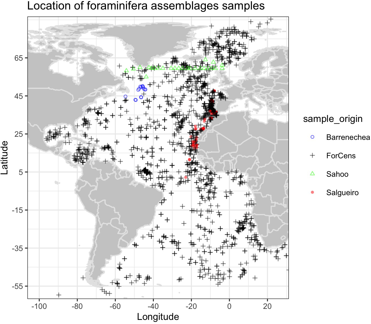
Map with location of the used sediment samples.
Alpha diversity Indices
Biological diversity comprises two main aspects: species richness and evenness or equitability (Magurran, 2004). In ecological studies, both the total number of species (species richness, S), the Shannon-Wiener diversity index (H) and evenness index (E) are commonly used to estimate community diversity. Species richness can be defined as the total number of species encountered in a sample (S). Although species richness may depend on sample size, in this case, the use of census counts (in % of total counts) refutes that possibility as it departs from an equal sample size. Evenness describes the distribution of individuals among the species, i.e. it is “Even” if all species (yet if few) are equally abundant (“even”/more diverse), or “uneven” if the community is dominated by one or a few species only (less diverse). To measure community evenness, the Probability of Interspecific Encounter (E) (Hurlbert, 1971), also known as Simpson’s evenness index and Gini-Simpson index, was used. The E index is unbiased relatively to sample size, and it represents the probability that two randomly chosen individuals from an assemblage will represent two different species. According to Gotelli and Ellison (2004), this index produces easily interpretable units of probability and corresponds intuitively to a diversity measure that is based on the encounter of a novel species, and it varies between 0 and 1 (with 1 representing a community with all species equally abundant (perfectly even, and therefore no species is dominant over another) and 0 representing a highly uneven one, i.e. dominated by one single species). The alpha diversity indices were calculated using the Vegan package (Oksanen et al., 2020) in the R free software (http://www.r-project.org/) and predicted over the sampled area into a regular grid by applying the spatial model estimated variogram, using kriging interpolation, for each index separately (Bivand et al., 2008; Cressie and Wikle, 2011). Kriging has been proven to be amongst the best interpolation methods to represent marine species distributions, when only geographical variables are considered (Rufino et al., 2021).
Oceanographic variables
In the current work, we compare foraminifera assemblages and the calculated diversity with SST, Chl-a concentration (as a surrogate for photosynthetic biomass) and EKE, all variables that can be approximated by satellite synoptic measurements at a large scale (Figure 2).
Figure 2
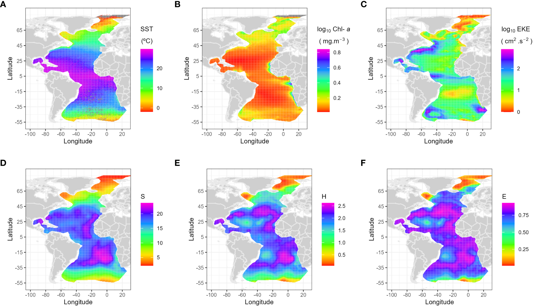
Geographic distribution of the main oceanographic drivers (annual averaged decadal scales), (A) Sea Surface Temperature (SST, °C), (B) Chlorophyll-a (CHL, mg m-3), (C) Eddy Kinetic Energy (EKE, cm2 s-2) with the latter two presented on logarithmic scale, and geographic distribution of the three diversity indices, interpolated using kriging, (D) species richness (S), (E) Shannon diversity (H) and (F) for evenness (E).
Annual averaged SST was extracted from the World Ocean Atlas 2013 (WOA13: Garcia et al. (2014)), which is a set of objectively analyzed (0.25° grid) climatological fields. The used variables correspond to the average of five “decadal” climatologies: 1955-1964, 1965-1974, 1975-1984, 1985-1994, and 1995-2006. Although salinity and nutrients in WOA13 (such as phosphate, nitrate, silicate) were initially considered in a preliminary analysis, we ended up not using them due to the strong collinearity with the selected variables (see Supplementary Figure 1).
Annual averaged Chl-a concentration (mg/m-3) is the product generated by the NASA Ocean Biogeochemical Model (NOBM) based on data assimilation of remotely sensed Chl-a. Garver–Siegel–Maritorena model bio-optical products were derived from SeaWiFS and MODIS-Aqua satellite data and processed by ICESS at the University of California – Santa Barbara (https://oceancolor.gsfc.nasa.gov).
The EKE per unit mass are the square of the velocities (cm2/s2) from the SSALTO/DUACS (Segment Sol multi-missions dALTimetrie, d’Orbitographie et de localisation précise/Data Unification and Altimeter Combination System) delayed-time level-4 product distributed by Copernicus Marine Environment Monitoring Service (https://resources.marine.copernicus.eu/product-detail/SEALEVEL_GLO_PHY_CLIMATE_L4_MY_008_057/INFORMATION). The sea level anomaly is the sea surface height above mean sea surface that is included in the absolute dynamic topography, and the mean was calculated over the 1993 – 2012 period. The velocities are geostrophic, estimated from the sea surface height anomaly (for the EKE) based on multi-satellite altimetry and thus should be interpreted as vertically averaged velocities dominated by the upper layer. Pseudo-streamlines are estimated from the geostrophic velocity field based on the absolute dynamic topography to provide a visualization of the mean currents (Supplementary Figure 2). EKE (log10 transformed) was therefore used as a proxy for ocean instability and mixing (Qiu et al., 2014; Uchida et al., 2017) and the streamlines mark the presence of currents and fronts associated to them. In fact, EKE marks the subtropical gyres western boundary currents: the Gulf Stream with onset of the North Atlantic Drift (and may be some interaction with the Labrador Current off Newfoundland); the Malvinas Current/Brazil-Malvinas Confluence Zone and parts of the Antarctic Circumpolar Current; the onset of the South Atlantic Current; the North Equatorial Counter Current and less strong the South Equatorial Current; and the Agulhas “leakage” around South Africa.
Statistical analysis of diversity indices
The relationship between the alpha diversity indices (H, S and E) and the oceanographic variables SST, Chl-a and EKE used here as explanatory variables or covariates, was statistically analyzed using a generalized additive mixed model (GAMM) approach. EKE and Chl-a were log10 transformed to stabilize the variances, i.e. lx = log10 (x+1) (a base of 10 was used to facilitate the interpretation). For H diversity, ‘Gaussian’ distribution was used, whereas for S (counts of species), the ‘Tweedie’ distribution was considered, since according to Wood et al. (2016), it is suitable for count data (using an estimated power of 1.01) and followed by the checking of the residual’s analyses. For E, a Beta distribution was used, with a logit function family, as recommended for proportions between [0,1]. The assumption of the lack of collinearity was tested (correlation between covariates) by estimating Spearman’s correlation coefficient between the three explanatory variables considered, and it was found that these were always below 0.7, which is the recommended rule of thumb (Zuur et al., 2010).
Spatial autocorrelation implies that samples that are closer to each other are more related than samples that are farther apart and therefore, are not independent, as assumed by most statistical models. To account for spatial autocorrelation, a statistical smoothing term was incorporated in the model as a random effect. In the H and S indices analysis, three spatial auto-correlation structures were evaluated for the random part of the model (exponential, spherical and, Gaussian), and, for each case the most appropriate one was selected using Akaike’s information criterion residuals distribution analysis and ‘acf’ and performance measurement criteria. In the case of Evenness, a term was added to the model, encompassing both latitude and longitude to account for the spatial component, since the use of Beta family did not permit the inclusion of a spatial autocorrelation structure (Wood, 2006).
In all cases, a full model was initially estimated using the three covariates, which was then subject to a model selection procedure, that included the interactions between terms. The best combination determined for each index based on Akaike’s information criterion (Zuur et al., 2010). Model assumptions were evaluated by analyzing the residuals distribution, including residuals auto-correlation (‘acf’) and covariates concurvity (to test collinearity) (Wood, 2006).
Species turnover analysis
Gradient forest analysis (GF) is a method that has been proven to be highly robust and efficient in identifying broad-scale environmental gradients of biodiversity patterns (Leaper et al., 2011; Ellis et al., 2012; Pitcher et al., 2012). This method has been used to: determine thresholds in/as ecological indicators (Large et al., 2015; Waite et al., 2020); identify thresholds of anthropogenic change in marine communities (Couce et al., 2020) in genomics (Fitzpatrick and Keller, 2015); determine the major drivers of phytoplankton distribution in lakes (Roubeix et al., 2016). To consider multiple, co-occurring species in model fitting, a community-level model was used (Nieto-Lugilde et al., 2018). Within these the Gradient Forest Analysis (GF) was chosen because tree-based techniques are among the top performing technique for species distribution analysis that are capable of modeling nonlinear responses and interaction effects, and permit to identify species turnover thresholds along environmental gradients. Using a large set of independent data for evaluation, this technique was found to be highly effective at summarizing spatial variation in both the composition of species assemblages and species turnover (Stephenson et al., 2018). Gradient Forest analysis was therefore applied to the relative abundance of foraminifera and the three oceanographic satellite variables to estimate the location and importance of the community composition thresholds along environmental gradients in the Atlantic Ocean (Ellis et al., 2012). For this analysis, the species relative abundance was natural log transformed, after adding a constant of one (log1p R function). The GF (Pitcher et al., 2011; Ellis et al., 2012) is a machine-learning modeling technique that predicts the distribution of a taxon as a function of relevant environmental variables, on the basis of fitting an ensemble of regression or classification trees. That is, multiple random forest models are run for each taxon separately and then simultaneously trained together to represent the community. Standardized measurements of change along environmental gradients for all taxa are therefore performed simultaneously to analyze the combined results.
This information is used to build ‘response curves’: empirical functions of change in composition for each environmental variable. After accounting for the distribution of the data along the gradient of the predictor, thresholds for which significant changes of community composition take place can be identified for each of the predictive variables, using the frequency histograms of the values at which splits happen in the individual decision trees. Furthermore, GF allows for the quantification of the relative importance of the predictor variables by averaging them across all taxa. Community threshold is defined as the zone, the critical value(s), along an environmental gradient where sharp increases or decreases in the occurrence of several taxa boost a change in community composition.
Results from this analysis were then used to transform the environmental layers to represent biological space, using the oceanographic layers: SST, EKE and Chl-a. A principal component analyses (PCA), was also applied to the predictions, and the first three axis of the PCA scaled into RGB space (Red-Green-Blue) for mapping species turnover. In addition, the main biogeographic regions of planktonic foraminifera were estimated using the k-means cluster method. The number of cluster groups was selected using the Elbow method (Supplementary Figure 3). Further details on the method and applications can be found elsewhere (Ellis et al., 2012; Baker and Hollowed, 2014; Large et al., 2015; Nieto-Lugilde et al., 2018; Stephenson et al., 2018; Couce et al., 2020). All the analysis were done using the R libraries mgcv (e.g., Wood, 2011; Wood et al., 2016; Wood, 2017), the package gradientForest (Ellis et al., 2012), and the package NbClust (Charrad et al., 2014) and factoextra (Kassambara and Mundt, 2020), for the determination of the number of clusters. Visualization of the GAMMs was done with the aid of library ‘mgcViz’ (Fasiolo et al., 2018), in R software.
Results
Spatial patterns of diversity indices
Spatial auto-correlation on alpha diversity indices was studied for the three indices and the variograms fitted with a spherical model (model results: S: nugget = 4.367, sill = 68.146 and range = 24669.715 (which would be equivalent to a linear model); H: nugget = 0.036, sill = 0.145 and range = 1930.019; E: nugget = 0.002, sill = 0.021 and range = 1378.223; Supplementary Figure 4). Species richness (S – Figure 2) shows the lowest number of species in the Arctic Ocean (1-4 species), followed by the Nordic Seas (1-11 species). Between 50 °N and 50 °S, the Atlantic shows almost symmetrical bimodal diversity richness south and north of the equator, but peaking values appear between 25 °N – 25 °S (15 to 27 species). Shannon diversity (H – Figure 2) is lower than 1 (corresponding to < 10 species) only close to the poles. Evenness (E – Figure 2) shows that 90% of the samples have less than 0.5 of encounter probability, that is, the probability of finding the same foraminifera species twice is less than 50% in most of the area. Ninety-eight percent of the samples with an E < 50% contain < 10 species of planktonic foraminifera and were located closer to the poles (> 50 °N and > 50 °S). In summary, the centers of the subtropical gyres show lower diversity (H), a lower number of species (S), and lower E (i.e., more uneven species distribution). In contrast, the equatorial region and the northern and southern boundaries of the hemispheric subtropical gyres and the eastern boundary currents exhibit higher species richness, a more even distribution of species abundance (lower E), and a H distribution pattern closer to E than to S.
Drivers of diversity
The response of the alpha diversity indices to a heterogeneous environment represented by SST, Chl-a, and EKE showed that the best model for all three indices included was given by the following formula: index ~ s(l10EKE, sst.woa13) + s(Chla). Further, adding spatial structure to the analysis improved the performance of the model and drastically decreased residual spatial autocorrelation in S and H. For S, a spherical model was fitted (adj- R2 = 82%; Tweedie (1.25)), whereas for the H index, the best model also included a spatial exponential correlation structure (adj- R2 = 71%). Results of the GAMMs for H, S and E show similar patterns and can be found in Supplementary Figure 4. The effect of SST was the strongest one for all indices (S, H, E) and controlled the large diversity patterns. A significant interaction between SST and EKE indicates that the relationship between EKE and diversity changes across the SST ranges (depicted by the interaction panel color shade, from yellow to blue, while the black lines represent species richness variability through EKE and SST, as can be observed in the Supplementary Figure 5). All three alpha diversity indices show an almost linear slightly negative relationship with Chl-a, but less critical than the SST/EKE interaction.
Species turnover
In the current work, GF analysis successfully modeled the whole assemblage simultaneously and determined the thresholds associated with continuous environmental gradients, the main species contributing to those changes, and the inference of the principal regions of occurrence along the Atlantic. The model explains a large proportion of the foraminifera assemblage variability (R2 = 59%, obtained by adding the R2-values for all predictors). The most critical environmental variables for the model were SST (R2 = 29%), Chl-a (R2 = 19%) and EKE (R2 = 11%). The primary community thresholds for foraminifera species turnover appeared at 5-10 °C and 22-28 °C SST, 0.05-0.15 mg m-3 Chl-a and, 1.2-2.0 cm2 s-2 log10 EKE energy (Figure 3), respectively.
Figure 3
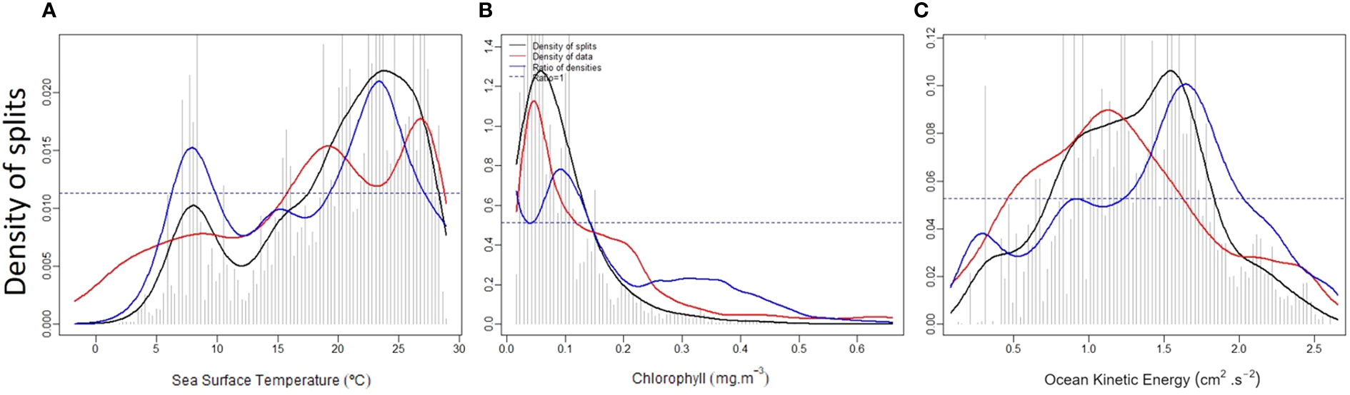
Binned split importance and location on each gradient (spikes), kernel density of splits (black lines), of observations (red lines), and splits standardized by observations density (blue lines) for the respective environmental parameters (A). Sea Surface Temperature (SST, °C), (B) Chlorophyll-a (CHL, mg m-3), (C) Eddy Kinetic Energy (EKE, cm2 s-2)). These show where essential changes in the abundance of multiple species are occurring along a variable gradient, i.e., indicate a composition change rate.
Out of the 37 foraminifera species considered in our combined dataset, only 28 (Supplementary Material) contributed to the species turnover model (Figure 4). The species not considered by the model corresponded to those whose maximum abundance was ≤ 2% in our data set. The response of each species to the different environmental variables presented in Figure 5, reveals that the most important species highlighted in each environmental gradient have R2 > 0.7 (Figure 4). From these, six species are also fundamental for transfer functions (Jonkers and Kučera, 2019), which further reinforces the results obtained and the analysis used. As expected, due to its dominance in polar waters, Neogloboquadrina pachyderma (purple in Figure 5; most relevant species in GF) is within the species that show marked thresholds relative to SST, with a sharp, pronounced transition between 7 and 9 °C. In contrast, the tropical species Trilobatus sacculifer (red; second most relevant species in GF) and Globigerinoides ruber (formerly Globigerinoides ruber pink; orange) mark the extreme warm threshold between 22 and 27°C. Neogloboquadrina incompta (blue), the third most important species (4th in GF), signals a more abrupt threshold at 7°C followed by a stepwise transition between 15 and 23°C. Globoconella inflata (green) shows thresholds at 10°C and 22°C.
Figure 4
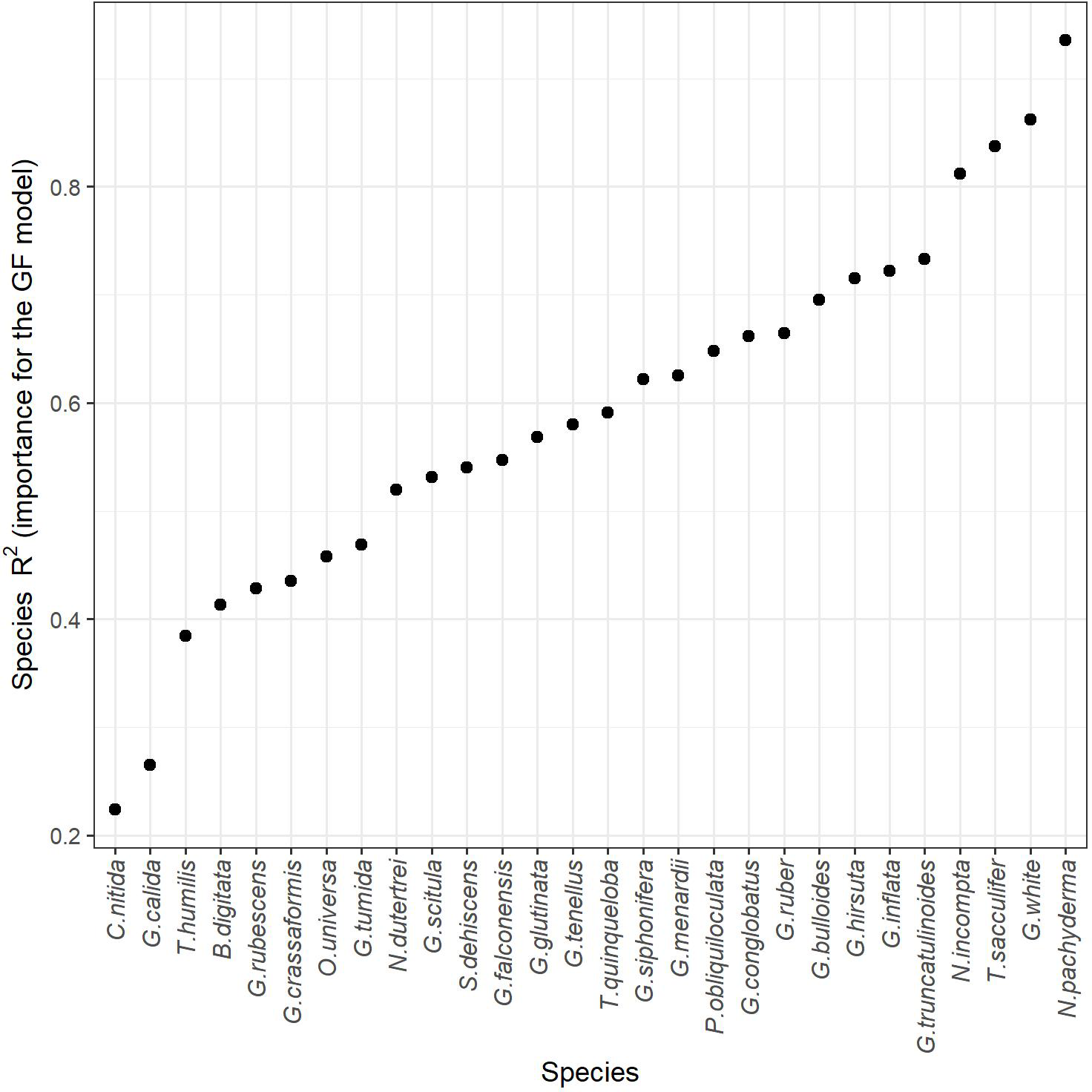
Importance of the foraminifera species (R2) for the turnover on the Gradient Forest Analysis (GF).
Figure 5
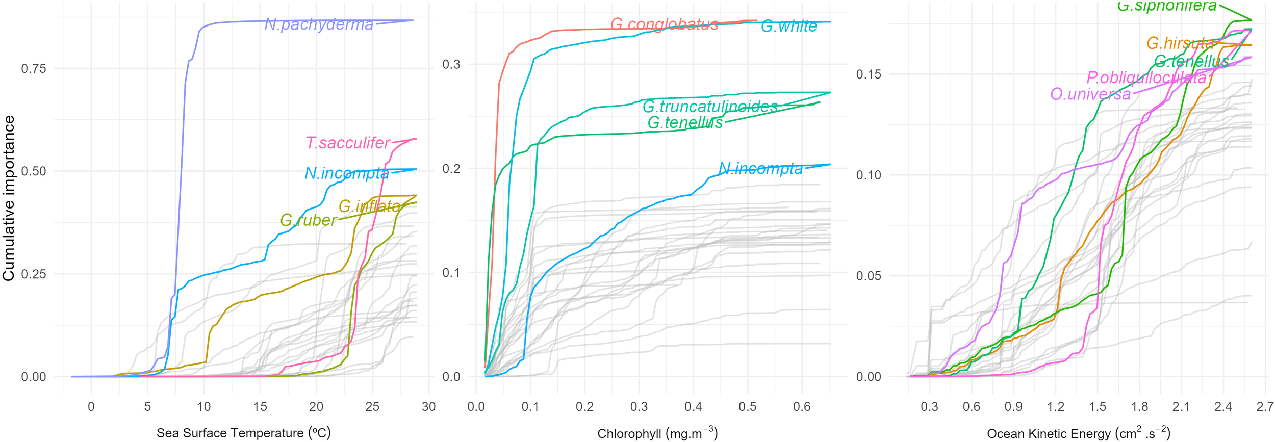
Cumulative change in abundance of individual foraminifera species, marking the values of the variable (Sea Surface Temperature (SST, °C), Chlorophyll-a (CHL, mg m-3), Eddy Kinetic Energy (EKE, cm2 s-2)), where changes occur, i.e., the values at which species change the most for each gradient. Legend is shown only for the topmost important five species in each gradient.
The most sensitive species to changes in Chl-a (Figure 5) are Globigerinoides white (formerly Globigerinoides ruber white) (green), Globigerinoides conglobatus (red), Globorotalia truncatulinoides (green-blue), Globigerinoides tenellus (olive green), and N. incompta (blue), all of these species with a R2 ≥ 0.6 for the GF model (Figure 4). Although all of them show thresholds below 0.1 mg m-3, subtropical species G. ruber, G. conglobatus and G. tenellus present the lowest (0.03 mg m-3) and more abrupt ones, followed by G. truncatulinoides with a more gradual transition between 0.04 and 0.11 mg m-3, whereas N. incompta shows a break at 0.09 followed by another, more gradual one at 0.4 mg m-3.
With respect to EKE, Pulleniatina obliquiloculata (dark pink), Globorotalia hirsuta (blue-green), Globigerinella siphonifera (green-brown), G. tenellus (olive green), and Orbulina universa (purple) show S-type relationships with steep thresholds but narrow intermediate plateaus (Figure 5). Their importance to the GF model (R2) exceeds 0.58, with the exception of O. universa with a value of 0.45 (Figure 4). G. tenellus, G. hirsuta and G. siphonifera behave similarly up to 0.9 cm2 s-2 followed by a clear divergence. G. tenellus shows steep slopes at 1 cm2 s-2 and 1.5 cm2 s-2, while G. hirsuta has an abrupt transition at 1.2 cm2 s-2 and then gradually increases until reaching a plateau at 2.4 cm2 s-2. G. siphonifera, on the other hand, continues the low slope increase up to 1.5 cm2 s-2, and then exhibits steep slopes at 1.7 cm2 s-2 and 2.1 cm2 s-2. P. obliquiloculata responds to EKE only above 1 cm2 s-2, and reveals a threshold at 1.4 cm2 s-2, followed by a less steep rise until 1.8 cm2 s-2 (Figure 5). O. universa reveals a steep increase until 0.9 cm2 s-2, followed by a slowly rising “plateau” between 0.9 and 1.6 cm2 s-2 and then another steep increase until 2.2 cm2 s-2.
When the species turnover map is transformed into the environmental space of the oceanographic variables and the bioregions are identified by cluster analysis (Figures 6A, B), not only the key latitudinal regions are visible, but the main current features are also superimposed; the eastern boundary upwelling systems (EBUS) off Namibia (Benguela Current) and Northwest Africa (Canary Current) as well as the Equatorial divergence, and the northern and southern subtropical fronts, i.e., the Gulf Stream-North Atlantic Drift path in the north, and the South Atlantic current in the south.
Figure 6
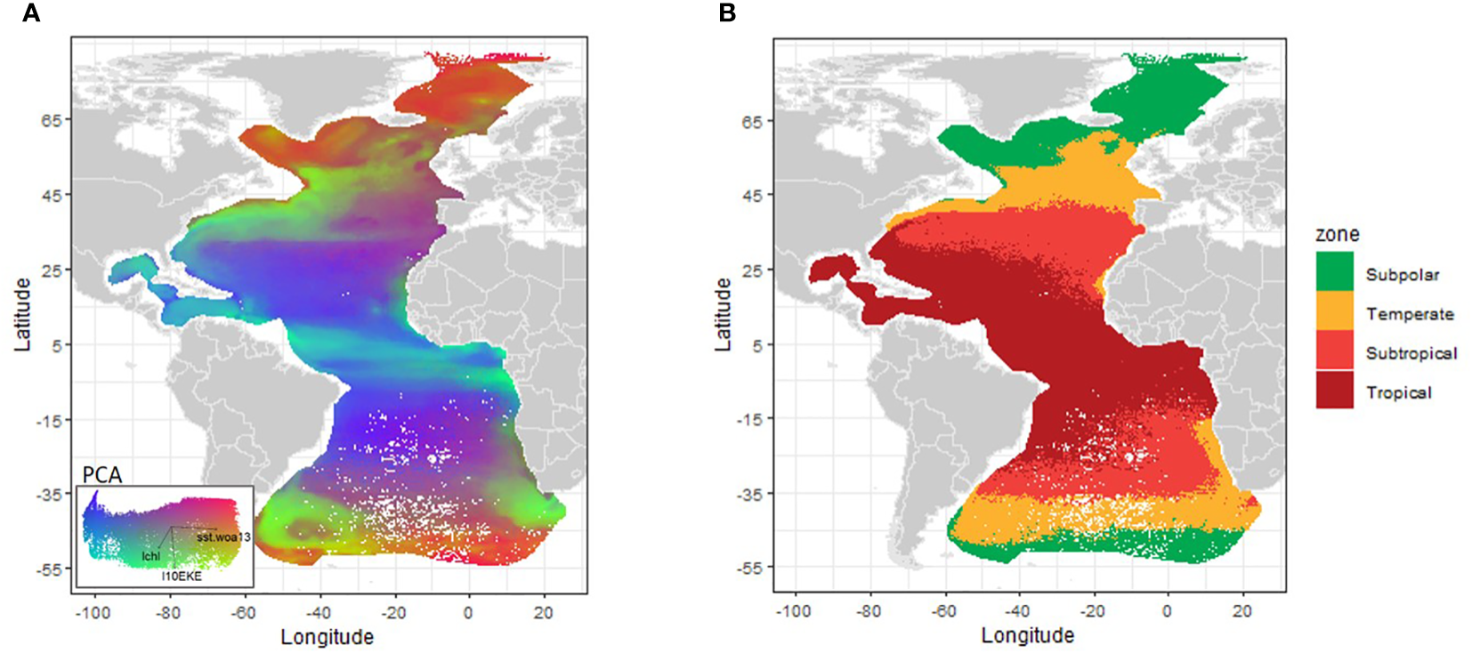
Changes of foraminifera community composition (species turnover) predicted by the Gradient Forest Analysis. These changes have been mapped over the first dimensions of a biologically transformed environmental space that accounts for their respective influence in dictating compositional patterns. (A) - map of species turnover and respective PCA; right panel: (B) - Map showing the spatial groups resulting of the k-means cluster analysis and corresponding zones (note the colors and names used are the same as in Kučera, 2007 to facilitate the comparison).(the geographic files of the zones are available upon request by email to the first author).
Discussion
Although the spatial distribution of diversity of planktonic foraminifera is likely to emerge from the operation of many different processes, the results of our statistical approaches (GAMM and GF analysis) confirm the importance of SST in controlling the variability in the diversity of planktonic foraminifera (~70%), in line with previous works (e.g., Rutherford and D'Hondt, 2000; Tittensor et al., 2010; Fenton et al., 2016; Rillo et al., 2022). However, they also reveal a significant effect of EKE (~20%), which becomes apparent on the geographic distribution of the various diversity related indices (Figure 2).
In the current work, kriging was used as an interpolation method to produce maps of diversity (without constraint by any environmental variable). The use of interpolated surfaces permits to better see the underlying patterns, especially when many samples may get overlaid, such as in Figure 3 by Fenton et al. (2016). Geostatistical techniques tend to produce smoother maps (unlike machine learning methods, for example, that produce scattered surfaces), which facilitate the identification of the large-scale processes and formulating the hypothesis tested in the current work. Fenton et al. (2016) estimated alpha diversity indices also using the ForCenS database, but used rarefaction to correct for sample size and extended the study to the whole ocean (Fenton et al., 2016 – Figures 3 vs. 2 in the current work). The species Richness distribution pattern is quite similar between the two studies, showing a drop towards the poles and a slight decrease at the Equator, contrasting with the highest values at mid-latitude gyres (20 – 25 °S and 25 – 30 °N) and along the NW Africa EBUS. Evenness or community diversity patterns resulting from our analysis shows a significant decrease in polar areas (>50° latitude). In contrast, the highest values strongly mark the major gyre boundaries and NW and SW African EBUS. In the current work we observed the same pattern in the S Atlantic than in Fenton et al. (2016), but the N Atlantic gyre limit is much less defined, possibly because more samples from that area were included in our extended dataset. Further, we have only used the Atlantic ocean (instead of the whole ocean) because we considered that the paucity of available samples in the other oceans would not permit to have the required resolution to test our hypothesis.
Impact of SST
The importance of SST as a driver for foraminifera’ diversity has been well shown in previous studies (e.g., Morey et al., 2005; Fenton et al., 2016; Rillo et al., 2022). Some authors, such as Fenton et al. (2016), attempted to evaluate the effect on the diversity of several environmental variables generally highly correlated with SST, namely nutrients and salinity. These studies did not provide additional information on the influence of ocean circulation nor studied SST thresholds for species turnover along environmental gradients. The present work reveals critical community thresholds at 5-10 °C and 22-28 °C SST, in agreement with previous observations, namely in transfer functions, and mainly related to Neogloboquadrina pachyderma and Neogloboquadrina incompta. Other than the preponderance of SST, the effect of a broader range of environmental factors have been hypothesized to explain local core top planktonic foraminifera diversity (e.g., Morey et al., 2005; Fenton et al., 2016; Rillo et al., 2022), but none of these authors considered proxies for ocean circulation. Only Richter et al. (2022) consider that plankton DNA biogeography at the global scale is linked to transport and large-scale ocean currents. Following this idea, we used EKE as a proxy of ocean fronts and circulation. SST, EKE, and Chl-a, which are all intrinsically connected with species physiology and ecology, and are likely to be the main drivers of foraminifera diversity. For example (1) SST, an index of solar energy input, influences the kinetics of biochemical reactions, metabolic rates and, thus, the probability of species mutation (Rhode, 1992; Allen et al., 2006; Eme et al., 2022), (2) Chl-a, as an index of productivity and food supply, determines population abundances, which are also directly related to the probability of mutation and species adaptation (Roy et al., 1998; Morey et al., 2005), and (3) kinetic energy, represented by EKE is a proxy for water column instability and ocean fronts, therefore it influences the rate of immigration and the probability of local extinction. These three variables reflect the main changes of energy between the individuals and the environment.
The maps of species turnover transformed to the environmental space of these oceanographic variables, and the resulting cluster groups (Figure 6), clearly show the major latitudinal regions known since the work of Bé (1959) and Bé and Tolderlund (1971). Since then, the defined bioregions and the location of the respective transition zones, i.e. boundaries with great faunistic contrast between zones, have been adapted and cited with very little changes, by many authors (e.g. Schmidt et al., 2004; Kučera, 2007; Rillo et al., 2022). In our study, only four provinces were identified, unlike previous works that describe five zones, probably because a large part of the fifth province, the polar zone (like in Schmidt et al. (2004) and Bé and Tolderlund, 1971), is in our study combined with the subpolar zone, potentially due to the exclusion of samples in the Antarctic polar region. Additionally, the upwelling areas in our study are not within the contiguous provinces (tropical and subtropical), but rather correspond to zones which are farther apart from the equator (i.e. temperate zone in Figure 6), unlike in Schmidt et al. (2004) where it is considered as a sixth province. Otherwise, the zones and location of transition areas found in our work purely using statistics are in good agreement with the planktonic foraminifera provinces already established by Bé and Tolderlund (1971) for the modern ocean, despite slight differences in the position of the borders of each province.
The central area around the equator corresponds to the tropical zone (Figure 6B). The north west corner coincides with previous works, being located near 38°N (as in Bé and Tolderlund, 1971; Schmidt et al., 2004 and refs. therein), but then diverges from those studies by the diagonal border down to 10°N off NW Africa, i.e., in our study the tropical zone in the eastern North Atlantic is greatly diminished. A similar pattern is observed for the boundary in the South Atlantic that also runs diagonally from about 15°S in the East to about 31°S in the West. Not only the diagonal shape, but also the latitude differs from previous works, with around 15-18°S in Schmidt et al. (2004) and Bé and Tolderlund (1971), whereas Rillo et al. (2022) place it up to 37°S. In fact, the south-west extension of the tropical zone in the South Atlantic in the current work largely overlaps with the subtropical zone (Figure 6B) in previous works. To sum up, in our study the subtropical zone gains area in the eastern North Atlantic and loses area in the western South Atlantic. The temperate zone (or transitional zone as termed in Bé and Tolderlund, 1971; Figure 6B), also marks the upwelling regions in our study, especially off SW Africa and in the Cape Blanc upwelling system (NW Africa). The south-west transition of the temperate zone is always located at the tip of South America (54°S), in agreement with the previous studies. The north-west temperate zone limit reaches up to 52°N in the southern Labrador Sea, whereas in previous definitions it was located near ~40°N, representing the beginning of the sub-polar zone (Figure 6B). The expansion of the temperate zone observed in this study in the North Atlantic can clearly be related to the influence of the North Atlantic Current and its branches (e.g., Daniault et al., 2016). Thus, the northern transition between sub-polar and temperate zone is further north in the current work, i.e., at 58°N, instead of 50°N in the previous works, whereas the transition between the temperate and subtropical zones is located further to the south (37°N vs. 42°N). The differences can be justified by the new samples included in the current study and by the statistical approach considered. Further work (and data, if possible) is required to improve the definition of the transition zones, potentially also integrating data from other taxonomic groups. Overall, there is a good correspondence between our and Rillo et al. (2022) borders of the polar and temperate bioregions, but not in the tropical and equatorial region, where our analysis clearly marks a subdivision of the two, aside from highlighting the significant circulation systems. Additionally, the provinces based on our species turnover also represent large circulation patterns and EBUS.
We believe that the location of the transitions of our bioregions improve the previous models due to higher accuracy in some aspects (e.g., reflecting main circulation pathways in the subtropical gyres). For example, in the Iberian margin where we added new samples by Salgueiro et al. (2008), the location of the transition between subtropical and temperate regions is found to be at 37°N (Cape São Vicente) and not at ~44°N as in previous works, which is in agreement with the local study of Salgueiro et al. (2008).
Impact of oceanographic currents, fronts and photosynthetic biomass
Bé and Tolderlund (1971) already concluded that the planktonic foraminifera characterize the major current systems of the world oceans, but quantitative analysis was not possible by then. For assessing the impacts of large-scale frontal systems on plankton foraminifera diversity we used EKE as it is the best currently available proxy at a large scale. However, further work is required in developing better proxies for this important variable to better verify their influence on marine diversity.
Differences in diversity are also depicted for EBUS. These systems, linked to the eastern boundary currents, lead to the occurrence of jets, filaments, and eddies that form along the Ekman divergence. However, their mesoscale variability is not depicted by altimetry, which is indeed known to be used to determine large-scale circulation (Cheney and Steel, 2001; Figure 2). Nevertheless, the Atlantic EBUS and the Equatorial Current system are clearly identified as biogeographic regions marked in the species turnover map (Figure 6), revealing the proliferation of opportunistic phytoplankton in response to the upwelling of nutrient-rich waters (Margalef, 1978; Raymont, 1980). In this scenario, ecological succession is followed by opportunist omnivorous and herbivorous planktonic foraminifera species, as reported in sediment trap studies (Abrantes et al., 2002; Schiebel et al., 2004) and reflected in species turnover.
Plankton foraminifera thresholds to SST, EKE and Chl-a gradients
When assemblage variability is accessed by GF, diverse morphologically defined species emerge with different importance and thresholds along the gradients of the environmental parameters identified as the main diversity drivers by our GAMM. For SST the most important species identified by GF (Figure 5 - N. pachyderma, T. sacculifer, N. incompta, G. inflata and G. ruber) are the same and appear in the same order of relevance as the ones driving transfer function results in the North and South Atlantic (Jonkers and Kučera, 2019). Furthermore, the thresholds revealed by GF for those species agree with the SST ranges used by Imbrie and Kipp (1971) to define the main planktonic foraminifera provinces: Tropical: ≥24 °C; Subtropical: 18 - 24 °C; Temperate/Transitional: 13 - 18 °C; Subpolar: 7 - 13 °C; and Polar: ≤ 7 °C. The fact that GF correctly identified the critical species and their temperature ranges, provides confidence to the results obtained by the same GF for Chl-a and EKE. Furthermore, it encourages us to validate if the compositional change marked by the individual species along each variable gradient can be explained by our current knowledge about the ecology of those species or can otherwise contribute to better understanding of their ecology. First, one can observe the species distribution pattern (Figure 7). N. pachyderma shows a polar to subpolar distribution justifying its low SST threshold. Similarly, T. sacculifer and G. ruber show a direct relation to tropical waters, also previously documented (e.g., Schiebel et al., 2002; Kučera, 2007). However, according to Schiebel and Hemleben (2017) and references therein, they spread over a wide range of SST and salinity, as suggested by the GF outcome (Figures 5, 7). N. incompta and G. inflata appear allied to intermediate SSTs (Figures 5, 7). The broad SST threshold from 15 to 22°C of N. incompta, a species with a single genotype in the Atlantic Ocean (Darling and Wade, 2008), is likely to reflect the diverse areas in which it thrives, from the mixing zone between the Gulf Stream and Labrador Current in the NW Atlantic, to the Canary and Benguela EBUS, where G. inflata also contributes considerably (Meggers et al., 2002; Lončarić et al., 2007; Salgueiro et al., 2008; Lessa et al., 2020). GF spotted thresholds for G. inflata fit with the broad range of subtropical to transitional waters inhabited by the species genotype I (Morard et al., 2011). However, the ramp between 5 and 10°C may reflect the association of its genotype II to the Antarctic subpolar waters (> 40°S) (Morard et al., 2011), in particular to the Malvinas Current in the SE Atlantic (Figure 7).
Figure 7
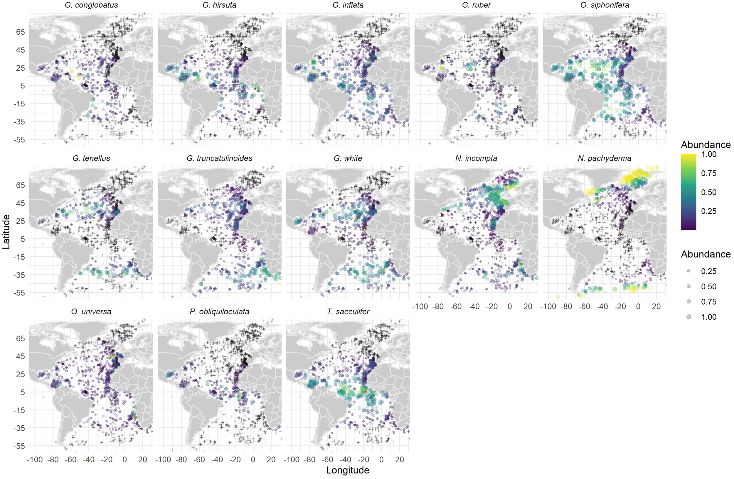
Spatial distribution and relative abundance of the 5 species with higher cumulative contribution in all environmental variables (abundance scale in both color and point size; crosses indicate zero abundance).
Considering Chl-a, the species identified by GF as the ones with a more substantial effect on community change along the Chl-a gradient are G. white, G. tenellus, G. conglobatus, G. truncatulinoides, and N. incompta (Figure 5). The three species with higher importance, G. white, G. conglobatus and G. tenellus, live in oligotrophic, subtropical to tropical waters (Rebotim et al., 2017; Schiebel and Hemleben, 2017; Jentzen et al., 2018; Lessa et al., 2020). Their distribution (Figure 7) displays an important presence along the Canary Current EBUS. In particular G. white, as reported by several authors (e.g., Meggers et al., 2002; Salgueiro et al., 2008), and that can explain the species higher Chl-a threshold relative to the other two species (Figure 5). The presence of G. white in both oligo- and eutrophic environments reflects the existence of two different genotypes identified in the Arabian Sea associated with eutrophic and oligotrophic conditions (Seears et al., 2012). The genotype preferring oligotrophic conditions also occurs in the subtropical North Atlantic and the Mediterranean Sea.
Based on the work of Morard et al. (2019)G. white, G. conglobatus and G. tenellus are genetically linked and that might be one of the reasons explaining their similar response to environmental variability in the GF analysis. As spinose species, they prefer to prey on zooplankton like copepods and ciliates, keeping them between their spines during feeding (Schiebel and Hemleben, 2017, and references therein). Contrarily, in laboratory cultures, neanic and juvenile specimens preferentially digest phytoplankton (Hemleben et al., 1989). In addition, all three species have dinoflagellates as photosymbionts (Hemleben et al., 1989; Takagi et al., 2019) and show a positive relationship between their test size and symbionts abundance (Takagi et al., 2019). Carrying photosynthetic symbionts enables them to develop better under higher nutrient conditions. Nevertheless, the fact that juveniles feed on phytoplankton may also suggest a relation of the most important spinose species with Chl-a and explain the lack of correlation between primary production and shell flux to the seafloor (Jonkers and Kučera, 2015).
The fourth species is the non-spinose species G. truncatulinoides, which, like other non-spinose species, is assumed to be omnivorous with a preference for herbivorous food (e.g., coccolithophores, diatoms) (Schiebel and Hemleben, 2017 and references therein). Although a deep-dwelling species, living below the thermocline in waters down to 600 m (e.g., Lončarić et al., 2006; Wilke et al., 2009; Ujiié et al., 2010; Jentzen et al., 2018), even reaching 2000 m water depths at the Azores Front (Schiebel et al., 2002), it migrated vertically up to the mixed layer, when it reproduces during winter (Hemleben et al., 1989; Wilke et al., 2009; Rebotim et al., 2017; Lessa et al., 2020). Furthermore, the G. truncatulinoides morphospecies incorporate four genotypes in the Atlantic Ocean with ecological niches extending from the polar-subantarctic waters in the South Atlantic to the North Atlantic subtropical gyre (de Vargas et al., 2001; Ujiié et al., 2010). This wide ecological range is picked up by the GF analysis (Figure 6B) and visible in Figure 7, with populations in the oligotrophic subtropical gyres and the Caribbean Sea likely associated with the lower Chl-a range up to 0.1 mg m-3 (see also Figure 2). Populations related to Chl-a between 0.1 and 0.3 mg m-3, on the other hand, likely relate to those thriving in the subantarctic Malvinas Current and the highly productive Brazil-Malvinas confluence zone in the Argentine basin as well as those profiting from enhanced productivity along the subtropical front in the South Atlantic, the Azores front in the North Atlantic and upwelling associated with the equatorial currents. Therefore, the association between subtropical-tropical G. truncatulinoides populations and Chl-a likely reflects the species reproduction strategy and is determined by the winter primary production maximum at those latitudes (e.g., Lévy et al., 2005).
The distribution of N. incompta (the last of the five-top species) includes the mid-latitudinal Atlantic, the subarctic/subantarctic domains, and the Atlantic province of the Nordic Seas (Figure 7), as previously reported (Johannesen et al., 1994; Boltovskoy et al., 1996; Schröder-Ritzrau et al., 2001; Schiebel and Hemleben, 2017). N. incompta is a species that tends to live below the Chl-a maximum (Field, 2004; Rebotim et al., 2017) and is assumed to be herbivorous as other non-spinose species (Hemleben et al., 1989). However, nothing is known about the food preferences of its genotype I. In the California Current EBUS, genotype II appears to graze on phytoplankton and prey on bacteria (Bird et al., 2018). The relationship of N. incompta with Chl-a (Figure 5) reveals breaks at 0.09 and 0.4 mg m-3. Compared with Figure 2, the populations of the Norwegian Sea and the sub-Antarctic domain are probably the ones responsible for the lower Chl-a range since higher fluxes to the seafloor are reported to occur only after the blooms in the hemispheric summer to early fall (Schröder-Ritzrau et al., 2001; King and Howard, 2003). As a result, populations inhabiting regions with Clh-a concentrations above 0.4 mg m-3, most probably will be those linked to the EBUS in the North and South Atlantic (Meggers et al., 2002; Salgueiro et al., 2008; Lessa et al., 2020).
The species that react the most to EKE variations are P. obliquiloculata, G. hirsuta, G. tenellus, G. siphonifera, and O. universa, reaching their highest importance above 2.4 cm2 s-2, whereas O. universa already starts to level out at 2.2 cm2 s-2 (Figure 5). These species distribution (Figure 7) at the latitudes of the equatorial current, counter- and undercurrent system and within the Caribbean Sea confirms that these species are strongly influenced by ocean currents and EKE. The occurrence of P. obliquiloculata and G. tenellus mainly in the area of the Gulf Stream (Figure 7) is particularly interesting as it justifies the species relationship to EKE values above 2.1 cm2 s-2.
Although with different importance, P. obliquiloculata and G. hirsuta, show EKE thresholds at 1.5 and 1.8 cm2 s-2 and 1.3 and 2.3 cm2 s-2, respectively. Both species are non-spinose, tropical to temperate and live in the intermediate-depth range (100-300 m; Schmuker and Schiebel, 2002; Wilke et al., 2009; Rebotim et al., 2017; Jentzen et al., 2018). P. obliquiloculata is associated with the deep Chl-a maximum (Schiebel and Hemleben, 2017 and references therein), and its higher fluxes to the seafloor occur in winter (Salmon et al., 2015). The fact that the equatorial currents and their branches that feed into the Caribbean Sea and the Gulf Stream extend into subsurface levels and thus into the depth range of this species, may explain its reaction to EKE (Figure 7). Although rare in the living fauna, this species has a high preservation potential in the sediment, which may result in an increase of its relative abundance in the sediment assemblage, and contribute to the GF identification over other tropical species like Globorotalia menardii and Neogloboquadrina dutertrei that are also known to be associated with the equatorial current system and the Gulf Stream (Fairbanks et al., 1980; Ufkes et al., 1998). G. hirsuta, on the other hand, feeds on diatoms and has an annual reproduction cycle similar to G. truncatulinoides, moving into subsurface waters in summer (Schiebel and Hemleben, 2017; Rebotim et al., 2017). In the North Atlantic, the species is associated with the southern side of the Azores front and Azores current (Storz et al., 2009; Rebotim et al., 2017), where its average living depth extends down to 400 m. Likewise, it exhibits higher abundances in the latitudes of the subtropical front in the South Atlantic (Figure 7). So, the gradual rise in importance to EKE values between 1.3 and 2.3 cm2 s-2 can clearly be linked to its affinities to those major frontal systems in both hemispheres.
Spinose species G. tenellus lives in the upper mixed surface layer (e.g., Rebotim et al., 2017; Jentzen et al., 2018) and contributes significantly to the assemblage of the subtropical gyre in the South Atlantic (Lessa et al., 2020). The lower range EKE thresholds (Figure 2) might reflect the high abundances observed between 15-20°S in the South Atlantic’s subtropical gyre (Figure 7). This species also occurs with similar abundances, in the Canary Current EBUS and along the major currents in the southwestern quadrant, which might explain the relation to higher EKE values (Figure 2).
Tropical to subtropical spinose, symbiont bearing, and omnivorous species G. siphonifera includes four genotypes with several subtypes and two morphotypes (Schiebel and Hemleben, 2017 and references therein), which are not distinguished in ForCenS. Not all of those subtypes occur in the Atlantic Ocean, and some of them are associated with particular oceanic regions or currents (Schiebel and Hemleben, 2017). That species genotypic variety seems to be reflected by the GF results. The linear response to 1.5 cm2 s-2 EKE appears to be related to the patch within the South Atlantic’s subtropical gyre or the subtropical gyres in general. Therefore, this group would include both cosmopolitan genotypes and those linked to the North Atlantic Drift, Azores and Canary Currents. The populations occurring after the break at 1.5 cm2 s-2 and the one at 2.1 cm2 s-2 are likely to encompass those living within the equatorial current and counter-current region, i.e., the same as observed for P. obliquiloculata, and those within the central and southern Caribbean Sea (Figure 7), i.e., mainly the tropical genotype associated with SST > 25°C (Schiebel and Hemleben, 2017). The third group, related to the highest EKE values, are composed of populations thriving within the Loop Current in the Gulf of Mexico and the Gulf Stream and potentially include the cosmopolitan genotype associated with SST > 17.5°C. The distribution of this group conforms to the high abundances observed by Fairbanks et al. (1980) in the slope waters and a cold-core ring, and the one solely observed in the North Atlantic Drift. Previous work has found that small cumulative changes in natural environmental parameters (e.g., shear stress), climate variables (e.g., temperature) and anthropogenic activities (e.g., bottom trawling) can lead to much larger responses than those predicted from linear effects on benthic biodiversity (Couce et al., 2020). Our results suggest a similar pattern also for plankton biodiversity.
Lastly, O. universa is a surface dwelling, mostly carnivorous species (e.g., Rebotim et al., 2017; Jentzen et al., 2018; Lessa et al., 2020). Three genotypes morphologically distinguishable based on shell thickness and pore size have been defined for this species (Morard et al., 2009; André et al., 2014; Marshall et al., 2015). Those geno-/morphotypes seem to have specific ecological preferences (Morard et al., 2009), which can be related to intervals in the cumulative importance curve (Figure 4). Genotype III (Mediterranean Sea) is the one more widely distributed in the Atlantic Ocean and linked to nutrient-rich waters (Morard et al., 2009). This variant contributes to EKE response throughout the wide range of 0.3 to 1.6 cm2 s-2, with the lower end reflecting the central part of the South Atlantic’s subtropical gyre (Figures 2, 5, 7). Due to its preference by nutrient-rich waters, we relate the higher O. universa abundances in the EBUS regions off western Iberia, NW and SW Africa (Figure 7) to the occurrence of this genotype and an EKE range from 1 to 1.6 cm2 s-2. Like for other species, the response at the upper end of the EKE spectrum, i.e., values above 1.6 cm2 s-2, is likely driven by the occurrences of genotypes I and II in the Caribbean Sea (genotype I), the equatorial current system and the Gulf Stream, where both genotype I and III are found (Morard et al., 2009). Genotype II is associated with the oligotrophic waters of the Sargasso Sea, and probably also contributes to the EKE range between 1 and 1.6 cm2 s-2 (Figures 2, 7).
In summary, our study reveals that planktonic foraminifera diversity in the Atlantic Ocean, and on a large scale, is not only determined by SST but also by EKE (currents) and Chl-a (photosynthetic biomass). Furthermore, the GF analysis allowed the redefinition of the location of the biogeographic transition zones (e.g., Bé and Tolderlund, 1971; Kučera, 2007), and identifies the species that most react to the variation of the different parameters. These results prompt the interest to use diversity indexes and the parameter-related species to attempt the definition of functions to reconstruct past EKE and Chl-a. Besides, the fact that large-scale ocean circulation is projected to change in response to climate warming calls for the use of diversity indexes to monitor such variations. Such monitoring could be achieved by combining the sampling of microplankton at specific locations along the encountered diversity gradients. Changes in latitude and/or longitude of those diversity gradients will reflect changes in the prevailing oceanographic circulation.
Conclusions
The analytical approaches applied to the expanded ForCenS dataset provide empirical evidence and statistical validation (GAMM and GF model) that, besides the strong SST effect found by several published works, there is a consistent effect of the ocean basin-scale circulation and its associated Chl-a (photosynthetic biomass) to the diversity of planktonic foraminifera in the Atlantic Ocean.
The application of GF permitted to identify the most relevant species and their thresholds relatively to SST, Chl-a, and EKE along each parameter’s gradient. A detailed study of individual species composition change rate may help shed light on their ecological behavior. Furthermore, similarly to the SST transfer functions, it opens the door to establishing quantitative proxies to reconstruct past Chl-a and EKE conditions.
Furthermore, future changes in the prevailing oceanographic features associated with climate warming might be exposed if monitored at specific locations along the latitudinal and longitudinal diversity gradients.
Funding
This study received Portuguese national funds from FCT - Foundation for Science and Technology through projects UIDB/04326/2020, UIDP/04326/2020 LA/P/0101/2020 and PTDC/AAG-GLO/3737/2012 and PINFRA/22157/2016 – EMSO-PT. MR was funded by FCT program Ciência 2007 and is currently funded by a DL57 associated with the project “Real-time monitoring of bivalve dredge fisheries” (MONTEREAL), Program MAR2020. AV was funded by FCT researcher contract IF/01500/2014 during the initial phase of the study. ES was funded by FCT SFRH/BPD/111433/2015 and PINFRA/22157/2016 – EMSO-PT.
Publisher’s note
All claims expressed in this article are solely those of the authors and do not necessarily represent those of their affiliated organizations, or those of the publisher, the editors and the reviewers. Any product that may be evaluated in this article, or claim that may be made by its manufacturer, is not guaranteed or endorsed by the publisher.
Statements
Data availability statement
Publicly available datasets were analyzed in this study. This data can be found at the PANGAEA DATA PUBLISHER under https://doi.org/10.1594/PANGAEA.873570; https://doi.org/10.1594/PANGAEA.878069; and https://doi.org/10.1594/PANGAEA.923299.
Author contributions
FA - Initial idea, discussed data, writing of the manuscript, secured the funds; MR – Conceptualization and methodology, statistical analysis, writing of the manuscript; ES – Assembled and revised the database, discussed data and revised the manuscript; PP – Calculated EKE and MKE and revised the manuscript; PC and AV discussed the data and revised the manuscript. All authors contributed to the article and approved the submitted version.
Conflict of interest
The authors declare that the research was conducted in the absence of any commercial or financial relationships that could be construed as a potential conflict of interest.
Supplementary material
The Supplementary Material for this article can be found online at: https://www.frontiersin.org/articles/10.3389/fmars.2022.887346/full#supplementary-material
References
1
Abrantes F. Meggers H. Nave S. Bollman J. Palma S. Sprengel C. et al . (2002). Fluxes of micro-organisms along a productivity gradient in the canary islands region (29 n): implications for paleoreconstructions. Deep-Sea Res. II49, 3599–3629. doi: 10.1016/S0967-0645(02)00100-5
2
Acha E. M. Mianzan H. W. Guerrero R. A. Favero M. Bava J. (2004). Marine fronts at the continental shelves of austral south America: Physical and ecological processes. J. Mar. Syst.44 (1–2), 83–105. doi: 10.1016/J.JMARSYS.2003.09.005
3
Allen A. P. Gillooly J. F. Savage V. M. Brown J. H. (2006). Kinetic effects of temperature on rates of genetic divergence and speciation. Proc. Natl. Acad. Sci. U.S.A.103, 9130–9913. doi: 10.1073/pnas.0603587103
4
André A. Quillévéré F. Morard R. Ujiié Y. Escarguel G. de Vargas C. et al . (2014). SSU rDNA divergence in planktonic foraminifera: Molecular taxonomy and biogeographic implications. PloS One9, e104641. doi: 10.1371/journal.pone.0104641
5
Angel M. V. (1991). Variations in time and space: Is biogeography relevant to studies of long-time scale change? J. .Marine Biol. Ass. U.K.71, 191–206. doi: 10.1017/S0025315400037504
6
Baker M. R. Hollowed A. B. (2014). Delineating ecological regions in marine systems: Integrating physical structure and community composition to inform spatial management in the eastern Bering Sea. Deep-Sea Res. Part II: Topical Stud. Oceanography109, 215–240. doi: 10.1016/j.dsr2.2014.03.001
7
Barrenechea Angeles I. Lejzerowicz F. Cordier T. Scheplitz J. Kučera M. Ariztegui D. et al . (2020). Planktonic foraminifera eDNA signature deposited on the seafloor remains preserved after burial in marine sediments. Sci. Rep.10:1–12. doi: 10.1038/s41598-020-77179-8
8
Bé A. W. H. (1969). “An ecological, zoogeographic, and taxonomic review of recent planktonic foraminifera,” in Oceanic micropaleontology. Ed. RamseyA. T. S. (London: Academic Press), 1–100.
9
Bé A. W. Hamlin W. S. (1967). Ecology of recent planktonic foraminifera - distribution in the north Atlantic during the summer of 1962. Micropaleontol.13 (1), 87–106. doi: 10.2307/1484808
10
Bé A. W. H. (1959). Ecology of Recent Planktonic Foraminifera: Part I: Areal Distribution in the Western North Atlantic. Micropaleontology5 (1), 77–100
11
Berger W. H. (1976). “Biogenous deep Sea sediments: Production, preservation and interpretation. chapter 29,” in Chemical oceanography, 2nd ed. Ed. Chester.J. (London: Academic Press).
12
Bé A. W. H. Tolderlund D. S. (1971). “Distribution and ecology of living planktonic foraminifera in surface waters of the Atlantic and Indian oceans,” in The micropaleontology of oceans (Cambridge, UK: Cambridge University Press).
13
Bird C. Darling K. F. Russell A. D. Fehrenbacher J. S. Davis C. V. Free A. et al . (2018). 16S rRNA gene metabarcoding and TEM reveals different ecological strategies within the genus neogloboquadrina (planktonic foraminifer). PloS One13 (1), e0191653. doi: 10.1371/journal.pone.0191653
14
Bivand R. S. Pebesma E. J. Gómez-Rubio V. (2008). Applied spatial data analysis with r. use r (Berlin: Springer-Verlag).
15
Boltovskoy E. Boltovskoy D. Correa N. Brandini F. (1996). Planktic foraminifera from the southwestern Atlantic (30 °–60 °S): species-specific patterns in the upper 50 m. Mar. Micropaleontology28 (1), 53–72. doi: 10.1016/0377-8398(95)00076-3
16
Brandão M. C. Garcia C. A. E. Freire ,. A. S. (2020). Meroplankton community structure across oceanographic fronts along the south Brazil shelf. J. Mar. Syst. 208 (103361), 1–14. doi: 10.1016/J.JMARSYS.2020.103361
17
Cermeño P. Falkowski P. G. (2009). Controls on diatom biogeography in the ocean. Science325 (5947), 1539–1541. doi: 10.1126/science.1174159
18
Charrad M. Ghazzali N. Boiteau V. Niknafs ,. A. (2014). NbClust: An r package for determining the relevant number of clusters in a data set. J. Stat. Software61 (6), 36. doi: 10.18637/jss.v061.i06
19
Chaudhary C. Saeedi H. Costello M. J. (2017). Marine species richness is bimodal with latitude: A reply to Fernandez and marques. Trends Ecol. Evol.32, 234–237. doi: 10.1016/j.tree.2017.02.007
20
Cheney R. E. Steel J. H. (2001). “Satellite altimetry,” in Encyclopedia of ocean sciences (Oxford: Academic Press).
21
Couce E. Engelhard G. H. Schratzberger M. (2020). Capturing threshold responses of marine benthos along gradients of natural and anthropogenic change. J. Appl. Ecol.57 (6), 1137:1148. doi: 10.1111/1365-2664.13604
22
Cressie N. Wikle C. K. (2011). Statistics for spatio-temporal data. Hoboken, NJ, USA: John Wiley and Sons. 624.
23
Daniault ,. N. Mercier H. Lherminier P. Sarafanov A. Falina A. Zunino P. et al . (2016). The northern north Atlantic ocean mean circulation in the early 21st century. Prog. Oceanography146, 142–158. doi: 10.1016/j.pocean.2016.06.007
24
Darling K. F. Wade C. M. (2008). The genetic diversity of planktic foraminifera and the global distribution of ribosomal RNA genotypes. Mar. Micropaleontology67 (3), 216–238. doi: 10.1016/j.marmicro.2008.01.009
25
de Vargas C. Renaud S. Hilbrecht H. Pawlowski J. (2001). Pleistocene adaptive radiation in globorotalia truncatulinoides: genetic, morphologic, and environmental evidence. Paleobiology27 (1), 104–125. doi: 10.1666/0094-8373(2001)027<0104:PARIGT>2.0.CO;2
26
Ellis N. Smith S. J. Pitcher C. R. (2012). Gradient forests: calculating importance gradients on physical predictors. ECOLOGY93, 156–168. doi: 10.1890/11-0252.1
27
Eme D. Rufino M. M. Trenkel V. M. Vermard Y. Laffargue P. Petitgas P. et al . (2022). Contrasted spatio-temporal changes in the demersal fish assemblages and the dominance of the and not fishing pressure, in the bay of Biscay and celtic Sea. Prog. Oceanography204, 102788. doi: 10.1016/J.POCEAN.2022.102788
28
Fairbanks R. G. Wiebe P. H. Bé A. W. H. (1980). Vertical distribution and isotopic composition of living planktonic foraminifera in the Western north Atlantic. Science207 (4426), 61–63. doi: 10.1126/science.207.4426
29
Falkowski P. G. Ziemann D. Kolber Z. Bienfang P. K. (1991). Role of eddy pumping in enhancing primary production in the ocean. Nature352 (6330), 55–58. doi: 10.1038/352055a0
30
Fasiolo M. Nedellec R. Goude Y. Wood S. N. (2018). Scalable visualisation methods for modern generalized additive models, ArXiv preprint arXiv:1809.10632.
31
Fenton I. S. Pearson P. N. Dunkley Jones T. Purvis A. (2016). Environmental predictors of diversity in recent planktonic foraminifera as recorded in marine sediments. PloS One11 (11), e0165522. doi: 10.1371/journal.pone.0165522
32
Field D. B. (2004). Variability in vertical distributions of planktonic foraminifera in the California current: Relationships to vertical ocean structure. Paleoceanography19 (2):1–22. doi: 10.1029/2003PA000970
33
Finlay B. J. (2002). Global dispersal of free-living microbial eukaryote species. Science296 (5570), 1061. doi: 10.1126/science.1070710
34
Fitzpatrick M. C. Keller S. R. (2015). Ecological genomics meets community-level modeling of biodiversity: mapping the genomic landscape of current and future environmental adaptation. Ecol. Lett.18 (1), 1:16. doi: 10.1111/ele.12376
35
Garcia H. E. Locarnini. R. A. Boyer T. P. Antonov J. I. Baranova O. K. Zweng M. M. et al . (2014). “World ocean atlas 2013, volume 4: Dissolved inorganic nutrients (phosphate, nitrate, silicate). s. levitus,” in NOAA Atlas NESDIS, 76. NODC: A. Mishonov Technical Ed.
36
Giamali C. Kontakiotis G. Koskeridou E. Ioakim C. Antonarakou A. (2020). Key environmental factors controlling planktonic foraminiferal and pteropod community’s response to late quaternary hydroclimate changes in the south Aegean Sea (Eastern Mediterranean). J. Mar. Sci. Eng.8 (9):1–23. doi: 10.3390/jmse8090709
37
Gotelli N. J. Ellison A. M. (2004). A primer of ecological statistics (Sunderland, MA: Sinauer Associates, Inc).
38
Hemleben C. Spindler M. Anderso O. (1989). Modern planktic foraminifera (Berlin: Springer).
39
Hillebrand H. Azovsky A. I. (2001). Body size determines the strength of the latitudinal diversity gradient. Ecography24 (3), 251–256. doi: 10.1034/j.1600-0587.2001.240302.x
40
Hillebrand H. Soininen J. Snoeijs P. (2010). Warming leads to higher species turnover in a coastal ecosystem. Global Change Biol.16, 1181–1193. doi: 10.1111/j.1365-2486.2009.02045.x
41
Hurlbert S. H. (1971). The nonconcept of species diversity: A critique and alternative parameters. Ecology52, 577:586. doi: 10.2307/1934145
42
Imbrie J. Kipp N. (1971). “A new micropaleontological method for quantitative paleoclimatology,” in Late Cenozoic glacial ages. Ed. TurekianK. (New Haven, Conn. USA: Yale University Press), 71–182.
43
Jentzen A. Schönfeld J. Schiebel R. (2018). Assessment of the effect of increasing temperature on the ecology and assemblage structure of modern planktic foraminifers in the Caribbean and surrounding seas. J. Foramin Res.48, 251–272. doi: 10.2113/gsjfr.48.3.251
44
Jing Z. Wang S. Wu L. Chang P. Zhang Q. Sun B. et al . (2020). Maintenance of mid-latitude oceanic fronts by mesoscale eddies. Sci. Adv.6 (31), eaba7880. doi: 10.1126/sciadv.aba7880
45
Johannesen T. Jansen E. Flatoy A. Ravelo A. (1994). “The relationship between surface water masses, oceanographic fronts and paleoclimatic proxies in surface sediments of the Greenland, Iceland, Norwegian seas,” in CArbon cycling in the glacial ocean: Constrains on the ocean's role in global change. Ed. ZahnR. (Berlin, Germany: Springer Verlag), 61–86.
46
Jonkers L. Kučera M. (2015). Global analysis of seasonality in the shell flux of extant planktonic foraminifera. Biogeosciences12, 2207–2226. doi: 10.5194/bg-12-2207-2015
47
Jonkers L. Kučera M. (2019). Sensitivity to species selection indicates the effect of nuisance variables on marine microfossil transfer functions. Clim. Past15, 881–891. doi: 10.5194/cp-15-881-2019
48
Kassambara A. Mundt F. (2020). “Extract and visualize the results of multivariate data analyses,” in R package version 1.0.7. Available at: https://CRAN.R-project.org/package=factoextra
49
King A. L. Howard W. R. (2003). Planktonic foraminiferal flux seasonality in subantarctic sediment traps: A test for paleoclimate reconstructions. Paleoceanography18 (1):19–17. doi: 10.1029/2002PA000839
50
Kučera M. (2007). “Planktonic foraminifera as tracers of past oceanic environments,” in Developments in marine geology, vol. Volume 1 . Eds. Hillaire–MarcelC.de VernalA. (Amsterdam, The Netherlands: Elsevier), 213–262.
51
Large S. I. Fay G. Friedland K. D. Link J. S. (2015). Quantifying patterns of change in marine ecosystem response to multiple pressures. PloS One10 (3):1–15. doi: 10.1371/journal.pone.0119922
52
Leaper R. Hill N. A. Edgar G. J. Ellis N. Lawrence E. Pitcher C. R. et al . (2011). Predictions of beta diversity for reef macroalgae across southeastern Australia. Ecosphere2 (7):1–18. doi: 10.1890/ES11-00089.1
53
Le Fèvre J. (1987). Aspects of the biology of frontal systems. Adv. Mar. Biol.23 (C), 163–299. doi: 10.1016/S0065-2881(08)60109-1
54
Lessa D. Morard R. Jonkers L. Venancio I. M. Reuter R. Baumeister A. et al . (2020). Distribution of planktonic foraminifera in the subtropical south Atlantic: depth hierarchy of controlling factors. Biogeosciences17 (16), 4313–4342. doi: 10.5194/bg-17-4313-2020
55
Lévy M. Lehahn Y. André J.-M. Mémery L. Loisel H. Heifetz E. (2005). Production regimes in the northeast Atlantic: A study based on Sea-viewing wide field-of-view sensor (SeaWiFS) chlorophyll and ocean general circulation model mixed layer depth. J. Geophysical Research: Oceans110 (C7):1–16. doi: 10.1029/2004JC002771
56
Lončarić N. Peeters F. J. C. Kroon D. Brummer G.-J. A. (2006). Oxygen isotope ecology of recent planktic foraminifera at the central Walvis ridge (SE Atlantic). Paleoceanography21 (3):1–18. doi: 10.1029/2005PA001207
57
Lončarić N. van Iperen J. Kroon D. Brummer G.-J. A. (2007). Seasonal export and sediment preservation of diatomaceous, foraminiferal and organic matter mass fluxes in a trophic gradient across the SE Atlantic. Prog. Oceanography73, 27:59. doi: 10.1016/j.pocean.2006.10.008
58
Longhurst A. R. (1981). Analyses of marine ecosystems (London: Academic Press).
59
Magurran A. (2004). Measuring biological diversity (Hoboken, NJ, USA: John Wiley & Sons).
60
Margalef R. (1978). Life-forms of phytoplankton as survival alternatives in an unstable environment. Oceanol. Acta1, 493–509.
61
Marshall B. J. Thunell R. C. Spero H. J. Henehan M. J. Lorenzoni L. Astor Y. (2015). Morphometric and stable isotopic differentiation of orbulina universa morphotypes from the cariaco basin, Venezuela. Mar. Micropaleontology120, 46–64. doi: 10.1016/j.marmicro.2015.08.001
62
Martin K. Schmidt K. Toseland A. Boulton C. A. Barry K. Beszteri B. et al . (2021). The biogeographic differentiation of algal microbiomes in the upper ocean from pole to pole. Nat. Commun.12 (1), 5483. doi: 10.1038/s41467-021-25646-9
63
Martiny J. B. H. Bohannan B. J. M. Brown J. H. Colwell R. K. Fuhrman J. A. Green J. L. et al . (2006). Microbial biogeography: putting microorganisms on the map. Nat. Rev. Microbiol.4 (2), 102–112. doi: 10.1038/nrmicro1341
64
McGillicuddy D. J. J. (2016). Mechanisms of physical-Biological-Biogeochemical interaction at the oceanic mesoscale. Annu. Rev. Mar. Sci.8 (1), 125–159. doi: 10.1146/annurev-marine-010814-015606
65
Meggers H. Freudenthal T. Nave S. Targarona J. Abrantes F. Helmke P. et al . (2002). Oceanic surface conditions recorded on the seafloor of the canary islands region through the distribution of geochemical and micropaleontological parameters. Deep-Sea Res. 49 (17), 3631–3654. doi: 10.1016/S0967-0645(02)00103-0
66
Morard R. Füllberg A. Brummer G.-J. A. Greco M. Jonkers L. Wizemann A. et al . (2019). Genetic and morphological divergence in the warm-water planktonic foraminifera genus globigerinoides. PloS One14, e0225246. doi: 10.1371/journal.pone.0225246
67
Morard R. Quillévéré F. Douady C. de Vargas C. de Garidel-Thoron T. Escarguel G. (2011). Worldwide genotyping in the planktonic foraminifer globoconella inflata: Implications for life history and paleoceanography. PloS One6 (10), e26665. doi: 10.1371/journal.pone.0026665
68
Morard R. Quillévéré F. Escarguel G. Ujiie Y. de Garidel-Thoron T. Norris R. D. et al . (2009). Morphological recognition of cryptic species in the planktonic foraminifer orbulina universa. Mar. Micropaleontology71, 148–165. doi: 10.1016/j.marmicro.2009.03.001
69
Morey A. E. Mix A. C. Pisias ,. N. G. (2005). Planktonic foraminiferal assemblages preserved in surface sediments correspond to multiple environment variables. Quaternary Sci. Rev.24 (7–9), 925–950. doi: 10.1016/J.QUASCIREV.2003.09.011
70
Munk P. Hansen B. W. Nielsen T. G. Thomsen ,. H. A. (2003). Changes in plankton and fish larvae communities across hydrographic fronts off West Greenland. J. Plankton Res.25 (7), 815–830. doi: 10.1093/PLANKT/25.7.815
71
Nieto-Lugilde D. Maguire K. C. Blois J. L. Williams J. W. Fitzpatrick M. C. (2018). Multiresponse algorithms for community-level modelling: Review of theory, applications, and comparison to species distribution models. Methods Ecol. Evol.9 (4), 834:848. doi: 10.1111/2041-210X.12936
72
Oksanen J. Guillaume Blanchet F. Friendly M. Kindt R. Legendre P. McGlinn D. et al . (2020). Vegan: Community ecology package. r package version. Available at: https://CRAN.R-project.org/package=vegan
73
Pitcher C. R. Ellis N. Smith S. J. (2011). Example analysis of biodiversity survey data with R package gradientForest. R vignette. 16. Available at http://gradientforest.r-forge.r
74
Pitcher C. Lawton P. Ellis N. Smith S. J. Incze L. S. Wei C. L. et al . (2012). Exploring the role of environmental variables in shaping patterns of seabed biodiversity composition in regional-scale ecosystems. J. Appl. Ecol.49 (3), 670:679. doi: 10.1111/j.1365-2664.2012.02148.x
75
Powell M. G. Beresford V. P. Colaianne B. A. (2012). The latitudinal position of peak marine diversity in living and fossil biotas. J. Biogeography39 (9), 1687–1694. doi: 10.1111/j.1365-2699.2012.02719.x
76
Qiu B. Chen S. Klein P. Sasaki H. Sasa Y. (2014). Seasonal mesoscale and submesoscale eddy variability along the north pacific subtropical countercurrent. J. Phys. Oceanogr44 (12), 3079:3098. doi: 10.1175/JPO-D-14-0071.1
77
Raymont J. (1980). Plankton and productivity in the oceans (Oxford: Pergamon Press).
78
Rebotim A. Voelker A. H. L. Jonkers L. Waniek J. J. Meggers H. Schiebel R. et al . (2017). Factors controlling the depth habitat of planktonic foraminifera in the subtropical eastern north Atlantic. Biogeosciences14 (4), 827–859. doi: 10.5194/bg-14-827-2017
79
Rhode K. (1992). Latitudinal gradients in species diversity: the search for the primary cause. OIKOS65, 514–527. doi: 10.2307/3545569
80
Richter D. J. Watteaux R. Vannier T. Leconte J. Frémont P. Reygondeau G. et al . (2022). Genomic evidence for global ocean plankton biogeography shaped by large-scale current systems. eLife11, e78129, doi: 10.7554/eLife.78129
81
Rillo M. C. Woolley S. Hillebrand H. (2022). Drivers of global pre-industrial patterns of species turnover in planktonic foraminifera. Ecography2022 (1):1–11. doi: 10.1111/ECOG.05892
82
Rodríguez-Ramos T. Marañón E. Cermeño P. (2015). Marine nano- and microphytoplankton diversity: redrawing global patterns from sampling-standardized data. Global Ecol. Biogeography24 (5), 527–538. doi: 10.1111/geb.12274
83
Roubeix V. Danis P. A. Feret T. Baudoin J. M. (2016). Identification of ecological thresholds from variations in phytoplankton communities among lakes: contribution to the definition of environmental standards. Environ. Monit. Assess.188 (4):1–20. doi: 10.1007/s10661-016-5238-y
84
Roy K. Jablonski D. Valentine J. W. Rosenberg G. (1998). Marine latitudinal diversity gradients: Tests of causal hypotheses. PNAS95 (7), 3699–3702. doi: 10.1073/pnas.95.7.3699
85
Ruddiman W. (1969). Recent planktonic foraminifera: Dominance and diversity in north Atlantic surface sediments. Science164, 1164–1167. doi: 10.1126/science.164.3884.1164
86
Rufino M. M. Albouy C. Brind'Amour A. (2021). Which spatial interpolators I should use? a case study applying to marine species. Ecol. Model.449:1–12. doi: 10.1016/j.ecolmodel.2021.109501
87
Rutherford S. D'Hondt S. (2000). Early onset and tropical forcing of 100,000 year pleistocene glacial cycles. Nature408, 72–75. doi: 10.1038/35040533
88
Rutherford S. D'Hondt S. Prell W. (1999). Environmental controls on the geographic distribution of zooplankton diversity. Nature400 (6746), 749–753. doi: 10.1038/23449
89
Sahoo N. Saalim S. M. Matul A. Mohan R. Tikhonova A. Kozina N. (2022). Planktic foraminiferal assemblages in surface sediments from the subpolar north Atlantic ocean. Front. Mar. Sci.8. doi: 10.3389/fmars.2021.781675
90
Salgueiro E. Voelker A. Abrantes F. Meggers H. Pflaumann U. Loncaric N. et al . (2008). Planktonic foraminifera from modern sediments reflect upwelling patterns off Iberia: Insights from a regional transfer function. Mar. Micropaleontology66, 135–164. doi: 10.1016/j.marmicro.2007.09.003
91
Salgueiro E. Voelker A. H. L. Martin P. A. Rodrigues T. Zúñiga D. Froján M. et al . (2020). δ18O and Mg/Ca thermometry in planktonic foraminifera: A multiproxy approach toward tracing coastal upwelling dynamics. Paleoceanography Paleoclimatology35 (2), e2019PA003726. doi: 10.1029/2019PA003726
92
Salmon K. H. Anand P. Sexton P. F. Conte M. (2015). Upper ocean mixing controls the seasonality of planktonic foraminifer fluxes and associated strength of the carbonate pump in the oligotrophic north Atlantic. Biogeosciences12, 223–235. doi: 10.5194/bg-12-223-2015
93
Schiebel R. Hemleben C. (2005). Modern planktic foraminifera. Paläontologische Z.79 (1), 135–148. doi: 10.1007/BF03021758
94
Schiebel R. Hemleben C. (2017). Planktic foraminifers in the modern ocean (Springer-Verlag: Berlin Heidelberg).
95
Schiebel R. Smart S. M. Jentzen A. Jonkers L. Morard R. Meilland J. et al . (2018). Advances in planktonic foraminifer research: New perspectives for paleoceanography. Rev. Micropaléontologie61 (3), 113–138. doi: 10.1016/j.revmic.2018.10.001
96
Schiebel R. Waniekb J. Zeltnera A. Alves M. (2002). Impact of the Azores front on the distribution of planktic foraminifers, shelled gastropods, and coccolithophorids. Deep-Sea Res. II49, 4035–4050. doi: 10.1016/S0967-0645(02)00141-8
97
Schiebel R. Zeltner A. Treppke U. F. Waniek J. J. Bollmann J. Rixen T. et al . (2004). Distribution of diatoms, coccolithophores and planktic foraminifers along a trophic gradient during SW monsoon in the Arabian Sea. Mar. Micropaleontology51 (3-4), 345–371. doi: 10.1016/j.marmicro.2004.02.001
98
Schmidt D. N. Renaud S. Schiebel R. (2004). Size distribution of Holocene planktic foraminifer assemblages : biogeography , ecology and adaptation. Mar. Micropaleontology50, 319–338. doi: 10.1016/S0377-8398(03)00098-7
99
Schmuker B. Schiebel R. (2002). Planktic foraminifers and hydrography of the eastern and northern Caribbean Sea. Mar. Micropaleontology46, 387–403. doi: 10.1016/S0377-8398(02)00082-8
100
Schröder-Ritzrau A. Andruleit H. Jensen S. Samtleben C. Schäfer P. Matthiessen J. et al . (2001). “Distribution, export and alteration of fossilizable plankton in the Nordic,” in The northern north Atlantic: A changing environment. Eds. SchäferP.RitzrauW.SchlüterM.ThiedeJ. (Berlin Heidelberg, Germany: Springer-Verlag).
101
Seears H. A. Darling K. F. Wade C. M. (2012). Ecological partitioning and diversity in tropical planktonic foraminifera. BMC Evolutionary Biol.12 (1), 54. doi: 10.1186/1471-2148-12-54
102
Siccha M. Kučera M. (2017). ForCenS, a curated database of planktonic foraminifera census counts in marine surface sediment samples. Sci. Data4 (1), 170109. doi: 10.1038/sdata.2017.109
103
Stehli F. G. Douglas R. G. Newell N. D. (1969). Generation and maintenance of gradients in taxonomic diversity. Science164 (3882), 947. doi: 10.1126/science.164.3882.947
104
Stephenson F. Leathwick J. R. Geange S. W. Bulmer R. H. Hewitt J. E. Anderson O. F. et al . (2018). Using gradient forests to summarize patterns in species turnover across large spatial scales and inform conservation planning. Diversity Distributions24 (11), 1641:1656. doi: 10.1111/ddi.12787
105
Storz D. Schulz H. Waniek J. J. Schulz-Bull D. E. Kučera M. (2009). Seasonal and interannual variability of the planktic foraminiferal flux in the vicinity of the Azores current. Deep Sea Res. Part I: Oceanographic Res. Papers56 (1), 107–124. doi: 10.1016/j.dsr.2008.08.009
106
Takagi H. Kimoto K. Fujiki T. Saito H. Schmidt C. Kučera M. et al . (2019). Characterizing photosymbiosis in modern planktonic foraminifera. Biogeosciences16, 3377–3396. doi: 10.5194/bg-16-3377-2019
107
The Ring Group (1981). Gulf stream cold-core rings: Their physics, chemistry, and biology. Science212 (4499), 1091. doi: 10.1126/science.212.4499.1091
108
Tittensor D. P. Mora C. Jetz W. Lotze H. K. Ricard D. Berghe E. V. et al . (2010). Global patterns and predictors of marine biodiversity across taxa. Nature466 (7310), 1098–1101. doi: 10.1038/nature09329
109
Uchida T. Abernathey R. Smith S. (2017). Seasonality of eddy kinetic energy in an eddy permitting global climate model. Ocean Model.118, 41–58. doi: 10.1016/j.ocemod.2017.08.006
110
Ufkes E. Jansen J. H. F. Brumrner G.-J. A. (1998). Living planktonic foraminifera in the eastern south Atlantic during spring: indicators of water masses, upwelling and the Congo (Zaire) river plum. Mar. Micropaleology33, 27–53. doi: 10.1016/S0377-8398(97)00032-7
111
Ujiié Y. de Garidel-Thoron T. Watanabe S. Wiebe P. de Vargas C. (2010). Coiling dimorphism within a genetic type of the planktonic foraminifer globorotalia truncatulinoides. Mar. Micropaleontology77 (3), 145–153. doi: 10.1016/j.marmicro.2010.09.001
112
van Sebille E. Scussolini P. Durgadoo J. V. Peeters F. J. C. Biastoch A. Weijer W. et al . (2015). Ocean currents generate large footprints in marine palaeoclimate proxies. Nat. Commun.6 (6521):1–8. doi: 10.1038/ncomms7521
113
Villa Martín P. Buček A. Bourguignon T. Pigolotti S. (2020). Ocean currents promote rare species diversity in protists. Sci. Adv.6 (29), eaaz9037. doi: 10.1126/sciadv.aaz9037
114
Voelker A. H. L. Salgueiro E. (2017). Planktonic foraminifera assemblages in NE Atlantic and alboran Sea surface sediments. PANGAEA. doi: 10.1594/PANGAEA.878069
115
Waite I. R. Pan Y. Edwards P. M. (2020). Assessment of multi-stressors on compositional turnover of diatom, invertebrate and fish assemblages along an urban gradient in pacific Northwest streams (USA). Ecol. Indic.112, 106047. doi: 10.1016/j.ecolind.2019.106047
116
Wilke I. Meggers H. Bickert T. (2009). Depth habitats and seasonal distributions of recent planktic foraminifers in the canary islands region (29°N) based on oxygen isotopes. Deep Sea Res. Part I: Oceanographic Res. Papers56 (1), 89–106. doi: 10.1016/j.dsr.2008.08.001
117
Wood S. N. (2006). Generalized additive models: an introduction with r (London, UK: Chapman and Hall/CRC).
118
Wood S. N. (2011). Fast stable restricted maximum likelihood and marginal likelihood estimation of semiparametric generalized linear models. J. R. Stat. Soc. (B)73, 3:36. doi: 10.1111/j.1467-9868.2010.00749.x
119
Wood S. N. (2017). Generalized additive models: An introduction with r. 2nd edition (London, UK: Chapman and Hall/CRC).
120
Wood S. N. Pya N. Säfken B. (2016). Smoothing parameter and model selection for general smooth models. J. Am. Stat. Assoc.111 (516), 1548–1563. doi: 10.1080/01621459.2016.1180986
121
Yasuhara M. Wei C.-L. Kučera M. Costello M. J. Tittensor D. P. Kiessling W. et al . (2020). Past and future decline of tropical pelagic biodiversity. Proc. Natl. Acad. Sci.117 (23), 12891. doi: 10.1073/pnas.1916923117
122
Zuur A. F. Ieno E. N. Elphick C. S. (2010). A protocol for data exploration to avoid common statistical problems. Methods Ecol. Evol.1 (1), 3–14. doi: 10.1111/j.2041-210X.2009.00001.x
Summary
Keywords
diversity, planktonic foraminifera, Atlantic Ocean, Chl-a, SST, kinetic energy
Citation
Rufino MM, Salgueiro E, Voelker AAHL, Polito PS, Cermeño PA and Abrantes F (2022) Ocean kinetic energy and photosynthetic biomass are important drivers of planktonic foraminifera diversity in the Atlantic Ocean. Front. Mar. Sci. 9:887346. doi: 10.3389/fmars.2022.887346
Received
01 March 2022
Accepted
14 November 2022
Published
29 November 2022
Volume
9 - 2022
Edited by
Aleksandra M. Lewandowska, Tvärminne Zoological Station, University of Helsinki, Finland
Reviewed by
Raphael Morard, University of Bremen, Germany; Marina C. Rillo, University of Oldenburg, Germany
Updates
Copyright
© 2022 Rufino, Salgueiro, Voelker, Polito, Cermeño and Abrantes.
This is an open-access article distributed under the terms of the Creative Commons Attribution License (CC BY). The use, distribution or reproduction in other forums is permitted, provided the original author(s) and the copyright owner(s) are credited and that the original publication in this journal is cited, in accordance with accepted academic practice. No use, distribution or reproduction is permitted which does not comply with these terms.
*Correspondence: Marta M. Rufino, marta.m.rufino@gmail.com; Fatima Abrantes, fatima.abrantes@ipma.pt
This article was submitted to Global Change and the Future Ocean, a section of the journal Frontiers in Marine Science
Disclaimer
All claims expressed in this article are solely those of the authors and do not necessarily represent those of their affiliated organizations, or those of the publisher, the editors and the reviewers. Any product that may be evaluated in this article or claim that may be made by its manufacturer is not guaranteed or endorsed by the publisher.